Abstract
Gradient accumulation enables training large-scale deep learning models under GPU memory constraints by aggregating gradients across multiple microbatches before parameter updates. Standard gradient accumulation treats all microbatches uniformly through simple averaging, implicitly assuming that all stochastic gradient estimates are equally reliable. This assumption becomes problematic in non-convex optimization where gradient variance across microbatches is high, causing some gradient estimates to be noisy and less representative of the true descent direction. In this paper, FracGrad is proposed, a simple weighting scheme for gradient accumulation that biases toward recent microbatches via a power-law schedule derived from a discretized Riemann–Liouville integral. Unlike uniform summation, FracGrad reweights each microbatch gradient by , controlled by . When , standard accumulation is recovered. In experiments on mini-ImageNet with ResNet-18 using up to accumulation steps, the best FracGrad variant with improves test accuracy from 16.99% to 31.35% at . Paired t-tests yield .
1. Introduction
Training large-scale deep neural networks has become increasingly memory-intensive, with modern models often requiring hundreds of gigabytes of GPU memory for a single training batch. Gradient accumulation has emerged as a standard technique to address this constraint, enabling training on memory-limited hardware by splitting each effective batch into smaller microbatches and accumulating their gradients before performing parameter updates. This approach maintains the same effective batch size while reducing peak memory consumption, making it possible to train models that would otherwise be infeasible on available hardware. Gradient accumulation is now widely used across diverse applications, from large language model pretraining to high-resolution image generation, and has become an essential component of modern deep learning infrastructure [1,2,3,4,5,6,7,8]. Although gradient accumulation preserves the effective batch size, it implicitly assumes that each microbatch gradient is an equally reliable estimate of the true gradient at the same parameter state . Standard gradient accumulation computes the accumulated gradient as where represents the gradient computed on the i-th microbatch and N denotes the number of accumulation steps. This uniform weighting scheme treats all gradient estimates equally. In reality, stochastic gradients computed on different random subsets exhibit high variance, especially in non-convex settings. Uniform averaging therefore gives equal weight to noisy microbatch estimates that may point away from the optimal descent direction [9,10,11]. Our key observation is that, even without parameter updates, later microbatches might yield less noisy gradient estimates simply by chance aggregation of data variance. That is, as more independent samples are drawn, the empirical average direction can converge slightly faster. This phenomenon is leveraged by applying a simple non-uniform reweighting of the microbatch gradients where recent microbatch estimates receive higher weight, while earlier estimates are down-weighted but not discarded. This study refers to this as biasing toward more reliable gradient estimates, rather than invoking staleness, which usually describes outdated gradients across parameter updates [12].
The problem of gradient variance becomes more severe as the number of accumulation steps increases. With larger N values, more microbatch gradients must be aggregated before a parameter update, increasing the likelihood that some gradient estimates are noisy or unrepresentative of the true descent direction. In stochastic optimization, the quality of individual gradient estimates varies significantly between different random microbatches. Despite the widespread use of gradient accumulation in memory-constrained training, existing methods do not account for this variance in gradient quality, continuing to aggregate gradients uniformly regardless of their reliability. This represents a limitation in current training practices, as the implicit assumption of equal gradient quality may break down when accumulation steps are large and gradient variance is high [6,8,9,13].
To the best of the author’s knowledge, no prior work has systematically investigated non-uniform weighting schemes for gradient accumulation that explicitly address gradient variance within accumulation cycles. While adaptive optimization methods such as Adam [14] and AdamW [15] employ exponential moving averages of gradients and second moments, these methods operate across parameter updates, maintaining state between optimization steps. In contrast, the gradient variance problem that this study identifies occurs within each individual accumulation cycle before any parameter update. Similarly, momentum-based methods like Polyak momentum [16] and Nesterov accelerated gradient [17] apply temporal weighting across multiple iterations rather than within single accumulation windows. This distinction is critical: existing adaptive methods address inter-update dynamics, whereas gradient accumulation requires intra-cycle aggregation strategies. The absence of principled temporal weighting mechanisms specifically designed for gradient accumulation under memory constraints represents a significant gap in current training methodologies, motivating this study’s investigation of fractional-order weighting derived from mathematical principles of temporal memory.
This study proposes Fractional Gradient Accumulation, or FracGrad, a simple weighting scheme for gradient accumulation that biases toward recent microbatches via a power-law schedule derived from a discretized Riemann–Liouville integral. Rather than treating all microbatches uniformly, FracGrad assigns higher importance to recent gradients while maintaining contributions from earlier gradients through power-law decay. Specifically, FracGrad computes weights as where controls the decay rate. When , the weights reduce to uniform values , recovering standard gradient accumulation. As decreases toward zero, the weighting becomes increasingly skewed toward recent microbatches, providing stronger recency bias [18,19,20,21].
The contributions of this work are as follows. First, this study identifys and formalize the gradient variance problem in standard gradient accumulation through both theoretical analysis and empirical evidence. This study demonstrates that uniform weighting of accumulated gradients is suboptimal when individual microbatch gradients exhibit high variance in non-convex optimization landscapes, and this study shows that this problem becomes increasingly severe as the number of accumulation steps grows larger. Our analysis establishes that existing gradient accumulation methods implicitly assume equal gradient quality across all microbatches, an assumption that fails to hold in practice when stochastic gradient estimates vary significantly in their reliability. Second, this study proposes Fractional Gradient Accumulation (FracGrad), a novel gradient accumulation method that applies fractional-order temporal weighting derived from the discretization of the Riemann–Liouville fractional integral. Unlike existing approaches that treat all accumulated gradients uniformly, FracGrad introduces power-law decay weighting that naturally balances recency bias with historical information retention through a single hyperparameter , where recovers standard accumulation and smaller values provide increasing recency emphasis. This represents the first application of fractional calculus principles to intra-cycle gradient weighting in deep learning optimization, providing a mathematically grounded framework for addressing gradient variance in memory-constrained training scenarios. Third, this study provides comprehensive experimental validation on mini-ImageNet with ResNet-18, demonstrating substantial improvements across multiple evaluation metrics. Our experiments show test accuracy improvements of up to 14.36 percentage points at sixteen accumulation steps, with statistical significance confirmed through paired t-tests yielding p-values of approximately . This study further demonstrates improvements in training stability through up to 20.2% reduction in gradient norm variance, faster convergence to target accuracy thresholds, and consistent benefits across different accumulation step values. Importantly, this study also analyzes the method’s limitations and failure modes, establishing its effective operating range at accumulation steps and identifying critical dependencies on optimizer choice that inform practical deployment guidelines [22,23,24,25].
2. Related Work
2.1. Gradient Accumulation and Memory-Efficient Training
Gradient accumulation enables training of large-scale models under GPU memory constraints by splitting each effective batch into N smaller microbatches and accumulating their gradients before performing parameter updates. The standard formulation computes the accumulated gradient as , where denotes the parameter state when processing the i-th microbatch and represents the loss on microbatch . This uniform averaging implicitly assumes that all gradient estimates are equally valid approximations of the true gradient at the current parameter state, which holds only when the loss surface is locally convex or when parameter changes during accumulation are negligible [9].
Gradient accumulation has become ubiquitous in modern large-scale deep learning systems. Megatron-LM [1] introduced comprehensive model parallelism techniques for training multi-billion parameter transformer language models, relying fundamentally on gradient accumulation to manage memory constraints across distributed GPU systems while maintaining large effective batch sizes. The training of GPT-3 [2] demonstrated the practical effectiveness of gradient accumulation at unprecedented scale, processing batch sizes of millions of tokens through thousands of accumulation steps distributed across hundreds of GPUs, yet maintaining the standard uniform averaging scheme throughout. ZeRO [3] optimizes memory efficiency by partitioning optimizer states, gradients, and parameters across multiple devices, enabling training of models with trillions of parameters, but continues to employ uniform gradient accumulation without modification to the aggregation weights. Mixed precision training [4] reduces memory footprint by performing forward and backward passes in FP16 arithmetic while maintaining master weights in FP32, dramatically decreasing memory consumption, yet this approach operates orthogonally to gradient accumulation and does not alter how gradients are aggregated within accumulation cycles. Gradient checkpointing [5] trades computation for memory by recomputing intermediate activations during backpropagation rather than storing them, enabling training of much deeper networks under memory constraints, but similarly maintains standard uniform gradient accumulation. These memory-efficient training techniques have enabled remarkable progress in large-scale model development, yet all share the common characteristic of treating gradient accumulation as a purely mechanical summation process without considering the varying quality of individual gradient estimates.
Large batch training methods investigate the relationship between batch size and learning rate scaling to maintain training dynamics when increasing effective batch sizes. These approaches typically employ linear scaling rules or adaptive warmup strategies to compensate for reduced gradient noise, but they fundamentally assume that gradients within each batch are aggregated uniformly. The key distinction is that large batch training addresses how to adjust hyperparameters when changing batch sizes, whereas this work addresses how to aggregate gradients within a fixed accumulation cycle when parameters evolve during that cycle [6,7,8,13,26].
Gradient checkpointing reduces memory consumption by trading computation for memory, recomputing intermediate activations during backpropagation rather than storing them. This technique is orthogonal to gradient weighting because it modifies how gradients are computed rather than how they are aggregated. Similarly, mixed precision training reduces memory footprint by performing forward and backward passes in lower precision arithmetic while maintaining a master copy of weights in full precision. Both methods maintain the standard uniform gradient aggregation scheme and do not address the temporal validity of gradients computed at different parameter states [3,4,5,27,28].
The fundamental limitation of existing memory-efficient training methods is that they treat gradient accumulation as a purely mechanical process of summing gradient vectors, ignoring the variance in gradient quality across different random microbatches. In stochastic non-convex optimization, individual microbatch gradients can be noisy and may not accurately represent the true descent direction. Our approach addresses this gradient variance problem by introducing principled temporal weighting that assigns higher importance to later gradients in the accumulation sequence, which may benefit from implicit information accumulation [9].
2.2. Adaptive Gradient Methods and Temporal Weighting
Adaptive optimization algorithms incorporate temporal information through exponential moving averages of gradients and second moments. Adam and AdamW maintain running averages with exponential decay and , providing adaptive learning rates per parameter. However, these methods operate across parameter updates, maintaining state between optimization steps, whereas FracGrad applies temporal weighting within each accumulation cycle before updates. Momentum methods like Polyak momentum and Nesterov accelerated gradient similarly use exponential weighting of historical gradients, but with fixed decay rates and across multiple iterations. The lookahead optimizer maintains slow and fast weight trajectories, again operating at the inter-update level. In contrast, FracGrad introduces intra-update temporal weighting with power-law rather than exponential decay, specifically targeting gradient variance within accumulation cycles. The power-law structure provides fundamentally different memory characteristics compared to exponential decay , with longer tails that preserve more information from earlier microbatches while still emphasizing recent gradients [10,11,14,15,16,17,29,30].
Although exponential weighting across updates is standard, less work has explored intra-cycle weighting. A natural baseline would be an exponential decay within the N microbatches, where controls the decay rate. The key distinction is that exponential decay assigns weights that decrease geometrically with distance from the most recent microbatch, while fractional power-law decay provides a more gradual transition that may better balance recency bias with historical information retention.
2.3. Fractional Calculus in Machine Learning
Fractional calculus has been explored in machine learning contexts, primarily through fractional derivatives in continuous optimization. Fractional gradient descent methods replace integer-order derivatives with fractional-order derivatives where , introducing non-local gradient information through integral operators. Fractional neural networks incorporate fractional activation functions or fractional-order dynamics in recurrent architectures. These approaches fundamentally modify the optimization landscape or model architecture through continuous fractional operators [18,19,20,21,31]. In contrast, FracGrad operates in discrete time, applying fractional-order weighting to pre-computed gradients rather than computing fractional derivatives. Our formulation derives from the Riemann–Liouville fractional integral discretization, but serves a distinct purpose: addressing gradient staleness in accumulation rather than modifying the loss surface. This makes FracGrad immediately applicable to any existing optimization algorithm without requiring specialized implementations or theoretical guarantees specific to fractional derivatives [18,19,20].
3. Background
3.1. Gradient Accumulation Fundamentals
Gradient accumulation is a technique that enables training of large neural networks under memory constraints by splitting each effective batch into smaller microbatches. Given a loss function parameterized by and an effective batch size B, standard mini-batch gradient descent computes the gradient over all B samples simultaneously. When memory is insufficient to process B samples at once, gradient accumulation divides the batch into N microbatches of size and accumulates their gradients before updating parameters. Formally, let denote the i-th microbatch for . The accumulated gradient is computed as
where represents the gradient computed on microbatch at the current parameter state . This formulation maintains the same expected gradient as processing the full batch B in one forward-backward pass, assuming the microbatches are sampled independently from the same distribution. The parameter update then follows the standard rule where is the learning rate.
The key property of standard gradient accumulation is that all microbatch gradients receive equal weight in the final aggregate. This uniform weighting is optimal when all gradient estimates have identical variance and are computed at the same parameter state. However, stochastic gradients exhibit high variance across different random samples, particularly in non-convex optimization. The implicit assumption that for all i holds in expectation, but individual realizations can deviate significantly. When gradient variance is high, some microbatch gradients may be noisy or unrepresentative, yet standard accumulation treats them identically to more reliable estimates. This motivates exploring non-uniform weighting schemes that can adapt to the varying quality of gradient estimates within an accumulation cycle.
3.2. Stochastic Gradient Estimation and Variance
In stochastic optimization, the gradient computed on a finite sample is an unbiased but noisy estimate of the true gradient. For a loss function and a random microbatch sampled from the data distribution, the stochastic gradient satisfies , but the variance can be substantial. This variance arises from two sources: the randomness in sampling data points and the inherent heterogeneity in the loss surface across different regions of the input space. In non-convex optimization, the variance is typically higher near saddle points and in regions where the Hessian has a large condition number.
The variance of the accumulated gradient under standard uniform weighting can be expressed as
where . When microbatches are sampled independently, the covariance terms vanish, yielding . If all microbatches have identical variance , this simplifies to , showing the standard variance reduction property of averaging. However, when individual gradient variances differ significantly, uniform weighting may not be optimal. Weighted averaging with weights satisfying yields variance
under independence. Minimizing this variance subject to the normalization constraint leads to optimal weights , which assign higher weight to lower-variance estimates. While computing exact variances is impractical during training, this principle suggests that non-uniform weighting can reduce aggregate variance when gradient quality varies across microbatches.
The fundamental question arises: why do stochastic gradients computed on different random microbatches exhibit high variance in non-convex optimization settings? This phenomenon stems from multiple interacting sources. First, data heterogeneity in the training distribution causes different samples to induce fundamentally different local loss surface geometries. When the loss function exhibits varying curvature across different regions of the input space, gradient estimates computed on different random subsets naturally point in divergent directions even when evaluated at identical parameter states. This heterogeneity is particularly pronounced in complex datasets where samples span diverse semantic categories, visual appearances, or linguistic structures. Second, local curvature variation in the loss landscape amplifies the sensitivity of gradient estimates to random sampling effects. Near saddle points, where some eigenvalues of the Hessian are close to zero while others remain large, small differences in sampled data can lead to drastically different gradient directions. Similarly, in regions where the Hessian has large condition numbers, the gradient direction becomes highly sensitive to noise, causing individual microbatch estimates to exhibit high variance even though their expectation remains unbiased. Third, batch size effects create a direct mathematical relationship between microbatch size and gradient variance, formalized by the relationship , where b denotes the microbatch size and represents the per-sample gradient variance. In memory-constrained training scenarios that necessitate gradient accumulation, microbatch sizes are necessarily small, often comprising only tens or hundreds of samples, which provides substantially noisier gradient estimates compared to large-batch training. In deep neural networks, these variance sources compound across layers through the chain rule of backpropagation, causing gradient variance at early layers to accumulate contributions from all subsequent layers, making gradient estimation particularly challenging when training with limited memory resources that require extensive gradient accumulation.
3.3. Fractional Calculus and Discrete Approximations
Fractional calculus extends classical calculus to non-integer orders of differentiation and integration. The Riemann–Liouville fractional integral of order for a function defined on is given by
where is the gamma function. The operator defined in (4) exhibits a power-law memory kernel that assigns decreasing weight to values of f at earlier times , with the decay rate controlled by . When , the operator reduces to standard integration. For , the kernel decays more slowly than exponential functions, providing longer memory of past values while still emphasizing recent information.
For discrete sequences, the Riemann–Liouville integral can be approximated using the Grünwald–Letnikov formulation. Given a discrete sequence with uniform spacing h, the fractional integral at position n is approximated by
where the weights are defined recursively by and
for . These weights decay approximately as for large k, exhibiting power-law behavior. An alternative discrete approximation uses the incremental form
for , which represents the contribution of position i to the fractional sum. These weights are normalized by to ensure that they sum up to unity. The incremental form provides a computationally efficient way to assign power-law decaying weights to a discrete sequence, with recent elements receiving higher weight when . This mathematical structure forms the basis for applying fractional-order weighting to gradient accumulation, where the discrete sequence corresponds to the ordered microbatch gradients within an accumulation cycle.
The Riemann–Liouville fractional integral possesses several important mathematical properties that make it particularly well-suited for gradient weighting applications in stochastic optimization.
Property 1 (Linearity): For any constants and integrable functions , the fractional integral satisfies the linearity property , which ensures that the weighted aggregation of gradients respects the linear structure of gradient spaces.
Property 2 (Composition rule): For fractional orders , the composition of fractional integrals satisfies the semigroup property , establishing that repeated fractional integration increases the total order additively.
Property 3 (Initial value behavior): The operator naturally incorporates initial conditions through the lower integration limit in the kernel , making it inherently suitable for discrete sequences with well-defined starting points such as the beginning of each gradient accumulation cycle.
Property 4 (Power-law decay): The power-law kernel decays asymptotically more slowly than exponential functions for any fixed decay constant , providing longer memory retention that prevents complete loss of early gradient information while still emphasizing more recent values. These mathematical properties collectively ensure that this study’s discrete weight formulation maintains mathematical consistency with the continuous fractional integral theory while providing computationally efficient implementation suitable for integration into modern deep learning training pipelines.
Among the various discrete approximations of fractional integrals available in numerical analysis literature, including the Grünwald–Letnikov method, the L1 finite difference scheme, and the trapezoidal rule approximation, this study adopts the Grünwald–Letnikov formulation for several compelling practical reasons. First and most importantly, the Grünwald–Letnikov discretization provides closed-form weight expressions that can be computed efficiently in time through simple arithmetic operations without requiring iterative numerical schemes or solving systems of equations. The incremental form presented in (7) emerges naturally and directly from this discretization, requiring only power operations and , subtractions, and a single normalization summation, making it highly practical for integration into existing training code. Alternative discretization schemes such as the L1 method, while potentially providing higher-order accuracy for smooth functions, would require solving tridiagonal or more complex linear systems at each accumulation cycle, introducing computational overhead that would dominate the gradient computation cost and defeat the purpose of lightweight gradient modification. The trapezoidal rule, while simple, does not preserve the characteristic power-law decay structure that motivates this study’s approach. Furthermore, the Grünwald–Letnikov method has been extensively validated in fractional calculus applications and provides stable numerical behavior for the fractional orders relevant to this study’s gradient weighting scheme.
This study clarifies an important indexing convention that appears in the recursive weight definition. In (6), the weight index k begins from with the base case , following standard conventions in fractional calculus literature. The recursive relation then generates subsequent weights for , producing the characteristic power-law decay pattern. This indexing starting from zero rather than one is essential for proper normalization of the discrete fractional operator and ensures numerical stability of the recursive computation. When applying these weights to this study’s gradient accumulation context, the weight corresponds to the gradient that is k steps in the past relative to the most recent microbatch.
A natural theoretical question arises regarding the choice between Riemann–Liouville and Caputo formulations of fractional calculus, both of which are widely employed in fractional differential equations and have distinct mathematical properties. This study choses the Riemann–Liouville fractional integral formulation over the Caputo fractional derivative for several reasons specific to this study’s gradient accumulation application. First, from a mathematical prerequisite standpoint, the Caputo fractional derivative requires that the function being differentiated possesses at least one classical derivative, imposing a smoothness assumption on the input sequence. In contrast, the Riemann–Liouville fractional integral operates directly on function values without requiring differentiability, which is a critical advantage when dealing with stochastic gradient sequences that exhibit high noise and do not satisfy smoothness assumptions. Stochastic gradients computed on random microbatches can vary dramatically between consecutive samples, violating the regularity conditions that Caputo derivatives assume. Second, from a computational structure perspective, the Riemann–Liouville integral produces a weighted sum structure directly through discretization, naturally yielding this study’s weight formula in (7) where each microbatch gradient receives a weight and the final aggregate is their weighted combination. The Caputo derivative, in contrast, would require computing finite differences of the gradient sequence before applying the fractional integration operator, introducing an additional layer of numerical differentiation that complicates implementation and potentially amplifies noise in stochastic gradient estimates. Third, from an application semantics viewpoint, the goal is to weight a discrete sequence of pre-computed gradients rather than to compute fractional derivatives of a continuous loss function with respect to a fractional-order parameter. The Riemann–Liouville integral’s convolution structure, which combines all past values with decaying weights, directly matches this weighting objective. The Caputo derivative’s primary advantage lies in its handling of initial conditions in fractional differential equations, where it allows specification of initial values in terms of integer-order derivatives that have direct physical interpretations. However, this advantage is less relevant in the gradient accumulation setting where all gradients are computed at the same fixed parameter state within each accumulation cycle, eliminating concerns about initial condition specification across parameter updates. While these theoretical considerations strongly favor the Riemann–Liouville formulation for this study’s application, this study acknowledges that investigating whether Caputo-based weighting schemes might provide benefits in alternative training scenarios, particularly those involving parameter drift during accumulation or online learning settings, represents an interesting direction for future theoretical research.
4. Method
4.1. Motivation and Problem Formulation
In modern deep learning training, gradient accumulation has become essential for training large-scale models under GPU memory constraints. The standard gradient accumulation procedure computes gradients over multiple microbatches and aggregates them before performing a parameter update. Formally, given N microbatches within an accumulation cycle, the standard approach computes the total gradient as a uniform average:
where denotes the gradient computed on the i-th microbatch. This uniform weighting scheme treats all microbatches equally, implicitly assuming that each gradient provides an equally valid estimate of the true gradient direction at the current parameter state.
From a numerical analysis perspective, the standard gradient accumulation formula in (8) implements a simple arithmetic mean of stochastic gradient estimates, which represents the maximum likelihood estimator under the assumption that all gradients are independent samples from an identical distribution with equal variance for all i. Under this equal-variance assumption, uniform weighting is provably optimal in the sense of minimizing the variance of the aggregate estimator , which achieves variance representing the standard convergence rate of Monte Carlo averaging. However, this optimality guarantee breaks down when the assumption of equal variance fails to hold, as occurs when individual microbatch gradients exhibit heterogeneous noise levels due to data heterogeneity, local curvature variation, or sampling artifacts. In such scenarios with unequal variances where varies with i, the classical minimum variance unbiased estimator theory establishes that weighted averaging with optimal weights inversely proportional to individual variances achieves lower aggregate variance than uniform averaging. Specifically, the optimal weighted estimator attains variance , which satisfies the inequality whenever variances differ, demonstrating strict improvement over uniform weighting. While computing exact variance for each microbatch during training is computationally impractical and would require maintaining extensive gradient statistics, FracGrad provides a computationally tractable proxy for variance-aware weighting by implementing the heuristic assumption that later microbatches in the accumulation sequence tend to provide lower-variance gradient estimates on average, operationalized through power-law weights rather than explicit variance estimation. This heuristic approximation enables practical variance reduction benefits without incurring the computational overhead of maintaining second-moment statistics or performing expensive variance computations.
However, this assumption may be suboptimal in stochastic non-convex optimization. During each accumulation cycle, parameters remain fixed while N microbatches are processed sequentially. Let denote the parameter state at the beginning of the accumulation cycle. All gradients are computed in the same state . The key issue is that each gradient is computed on a different random microbatch, leading to high variance in the gradient estimates. In non-convex optimization with stochastic gradients, individual microbatch gradients can be noisy and may not accurately represent the true descent direction. Our observation is that even without parameter updates, later microbatches might yield less noisy gradient estimates simply by chance aggregation of data variance. That is, as more independent samples are drawn within the accumulation cycle, the empirical average direction may converge slightly faster.
This study proposes to address this by introducing a weighting scheme based on fractional calculus. Rather than treating all gradients uniformly, this study assigns higher weights to more recent gradients while maintaining contributions from earlier ones through a power-law decay mechanism. This approach provides a mathematically grounded framework for biasing toward potentially more reliable gradient estimates. This study refers to this as biasing toward more reliable gradient estimates rather than invoking gradient staleness, which usually describes outdated gradients across parameter updates. Within a single accumulation cycle, there is no parameter shift, so the issue is variance in stochastic gradient estimates rather than staleness in the traditional sense.
To formalize the theoretical intuition behind why later microbatches in the accumulation sequence might provide more reliable gradient estimates despite all being computed at the identical parameter state , this study presents the following variance-based perspective. Let denote the gradient computed on the i-th random microbatch at the fixed parameter state. While all gradient estimates satisfy the unbiasedness property , they exhibit different realized variance due to the random sampling of training data. In the sequential gradient accumulation process, the act of observing gradients on preceding microbatches provides implicit information about the gradient variance structure in the current training state. Specifically, if the early gradient estimates exhibit high angular disagreement or magnitude variation, this serves as an empirical signal that the gradient variance is substantial in the current region of parameter space. By constructing a weighting scheme that down-weights earlier observed gradients and emphasizes later observations, FracGrad effectively implements an adaptive response to this variance structure without requiring explicit computation of variance estimates or second-moment statistics. This heuristic aligns with principles from online learning and sequential decision-making, where more recent observations often receive higher weight to enable adaptation to changing conditions. While the gradient accumulation setting involves a stationary data distribution within each cycle rather than genuine non-stationarity, the high variance of individual stochastic gradient estimates motivates similar temporal weighting principles. The power-law decay structure provides a principled mathematical framework for implementing this recency bias while maintaining contributions from all microbatches through the long-tail memory property of fractional integrals, avoiding the complete dismissal of early gradient information that would occur with more aggressive weighting schemes.
4.2. Fractional-Order Gradient Weighting
This study formulates Fractional Gradient Accumulation (FracGrad) by replacing the uniform averaging in (8) with fractional-order weighted aggregation. The FracGrad gradient is computed as:
where denotes the fractional weight assigned to the i-th microbatch gradient, and is a hyperparameter controlling the decay rate. The weights are derived from the fractional integral operator, which naturally produces power-law decay patterns that have proven effective in modeling systems with memory effects. The key distinction from standard accumulation is that FracGrad explicitly models the temporal ordering of microbatches within each accumulation cycle, assigning different importance to gradients based on their position in the sequence.
The fractional weights are defined using the Riemann–Liouville fractional integral formulation, adapted for discrete gradient accumulation. The Riemann–Liouville fractional integral of order for a continuous function is defined as:
where is the gamma function. For discrete gradient accumulation, this study discretizes this integral using the Grünwald–Letnikov approximation, which leads to weights proportional to . Specifically, this study computes the weights as:
The numerator represents the fractional increment for position i, while the denominator ensures proper normalization such that . This normalization guarantees that the magnitude of the accumulated gradient remains comparable to standard accumulation, preventing scale-related training instabilities. The normalization is critical because without it, the sum of weights would vary with , causing the effective learning rate to change unpredictably.
The FracGrad weighting scheme defined in (11) possesses several mathematically and practically desirable properties that distinguish it from ad-hoc or heuristic weighting approaches and establish its suitability for gradient accumulation in memory-constrained training.
Property 1 (Recency bias with memory): Unlike exponential decay weighting schemes where weights decrease geometrically and rapidly approach zero for distant past values, the power-law decay structure maintains non-negligible weights for all microbatches throughout the accumulation window. This longer memory tail prevents complete loss of gradient information from early microbatches while still emphasizing recent gradient estimates, providing a mathematically principled balance between utilizing historical information and adapting to recent observations. For instance, at with , the oldest microbatch still receives weight (approximately 2.5% of total), whereas an exponential scheme with comparable recent-to-old ratio would assign near-zero weight.
Property 2 (Smooth interpolation): The fractional order parameter provides continuous interpolation between uniform weighting ( yielding for all i) and increasingly aggressive recency bias as decreases toward zero. This smooth parameter space enables fine-grained control over the trade-off between temporal emphasis and historical retention, facilitating principled hyperparameter selection through standard tuning procedures rather than requiring discrete architectural choices.
Property 3 (Normalization preservation): The denominator in (11) ensures that weights sum exactly to unity, , for all values of and N. This normalization property maintains gradient magnitude consistency across different configurations and accumulation step values, preventing unintended learning rate scaling effects that would occur if the aggregate weight sum varied.
Property 4 (Scale adaptivity): The weights automatically adapt their decay rate to the number of accumulation steps N, with the power-law structure naturally spanning the full accumulation window regardless of its length. This scale-invariance property means that the relative emphasis on recent versus early gradients remains approximately constant across different memory constraint scenarios, unlike fixed exponential decay rates that would become increasingly severe as N grows.
Property 5 (Computational efficiency): Computing the complete weight vector for N microbatches requires arithmetic operations consisting of power evaluations, N subtractions, one summation, and N divisions, with total operation count approximately . For typical deep neural networks where the number of parameters ranges from millions to billions, this weight computation is completely dominated by the cost of computing N gradient vectors through forward and backward passes, rendering the fractional weighting overhead negligible in practice.
The parameter controls the degree of temporal weighting. When , the weights reduce to uniform values for all i, recovering standard gradient accumulation. This can be verified by direct computation: for all i, so the numerator is constant and the denominator equals N, yielding . As decreases to zero, the weighting becomes increasingly skewed towards recent gradients. For , the weights exhibit power-law decay, with increasing monotonically with i, meaning more recent microbatches receive progressively higher weights. To understand this behavior, note that for small , the function grows slowly, so is larger when i is large (corresponding to recent microbatches) because the derivative is larger for smaller x values. This power-law structure provides a smooth interpolation between uniform weighting and extreme recency bias, allowing fine-grained control over the temporal emphasis.
The implementation of FracGrad requires minimal modification to existing training pipelines. During each accumulation cycle, gradients are computed and stored as usual. Before calling the optimizer step function, this study computes the fractional weights using (11) and apply them to the accumulated gradients. The weight computation has complexity and involves only simple arithmetic operations, introducing negligible computational overhead compared to the gradient computation itself. Specifically, computing the weights requires N power operations, N subtractions, one summation, and N divisions, which is dominated by the cost of computing N gradients where denotes the number of model parameters. For typical deep learning models with millions to billions of parameters, the weight computation overhead is less than one percent of total training time. Importantly, FracGrad is completely optimizer-agnostic and architecture-agnostic, working seamlessly with any optimization algorithm such as Adam, SGD, or AdamW, and any model architecture including transformers, convolutional networks, and diffusion models. The method does not require modifications to the optimizer implementation or model architecture, making it immediately deployable in existing training pipelines.
4.3. Theoretical Analysis and Properties
Rather than a formal convergence guarantee, this study poses the following working hypothesis based on this study’s empirical observations.
Hypothesis (Empirical Effectiveness of FracGrad). In stochastic non-convex training with moderate gradient variance, reweighting microbatch gradients by the power-law schedule tends to reduce variance and yield improved optimization trajectories, provided is chosen sufficiently below 1 and the number of accumulation steps N does not exceed a practical threshold (here ).
This behavior aligns with known variance-reduction effects from weighted averaging in other stochastic methods. The key properties of FracGrad that support this hypothesis are as follows. First, gradient accumulation is widely used in modern large-scale training, making any improvement to this component immediately applicable across diverse applications. Second, FracGrad requires only a single-line modification to training loops, making it a simple intervention point in the training pipeline. The modification involves computing fractional weights once per accumulation cycle and multiplying them element-wise with the accumulated gradients before the optimizer step. Third, FracGrad is designed to be compatible with arbitrary optimizers and model architectures. The method operates purely on gradient vectors without making assumptions about the optimizer state or model structure. Fourth, it directly addresses the issue of gradient estimation quality during memory-constrained training.
To understand why FracGrad may improve gradient estimation, consider the stochastic gradient estimation problem. Let denote the loss function and denote the parameter state at the beginning of an accumulation cycle. All gradients are computed at this same state, where represents the i-th random microbatch. In stochastic optimization, individual microbatch gradients are noisy estimates of the true gradient . FracGrad assigns higher weights to later gradients in the sequence. While all gradients are computed at the same parameter state, the sequential observation of microbatches may provide information about gradient variance. By down-weighting earlier gradients and emphasizing later ones, FracGrad may reduce the impact of noisy gradient estimates.
The computational overhead of FracGrad is provably negligible. Computing the fractional weights requires arithmetic operations per accumulation cycle, which is dominated by the cost of gradient computation, where denotes the number of model parameters. For typical large-scale models with millions to billions of parameters, the weight computation represents less than one percent of the total training time. Specifically, the weight computation involves N power operations to compute and , N subtractions to compute the numerators, one summation over N terms to compute the denominator, and N divisions to normalize the weights. Modern hardware can perform these operations efficiently, and the weights can be precomputed once per accumulation cycle and reused for all parameter gradients. Memory overhead is similarly minimal, requiring only N additional scalar values to store the precomputed weights, which can be reused across training steps when N remains constant. This represents negligible memory consumption compared to storing the model parameters and optimizer states.
A critical theoretical question concerns why power-law decay weighting derived from fractional integrals should outperform alternative temporal weighting schemes such as exponential decay, which represents the most natural baseline comparison for time-dependent weighting. Exponential weights of the form for a decay factor also provide recency bias, assigning higher weight to recent microbatches through geometric decay. This study argues that power-law decay offers three fundamental advantages over exponential decay in the gradient accumulation context.
First, memory retention characteristics: Exponential decay with decay factor assigns weight to a gradient k steps in the past, which vanishes extremely rapidly. For example, with which already represents relatively slow decay, a gradient 10 steps in the past receives weight (approximately one-third of the most recent weight), and a gradient 20 steps in the past receives weight (approximately one-eighth of the most recent weight). By contrast, power-law decay with at assigns the oldest gradient weight compared to the newest weight , maintaining a ratio of approximately or roughly one-ninth rather than exponentially vanishing. More importantly, the collective weight assigned to the first half of microbatches under power-law decay remains substantial (approximately 20–30% for typical values), whereas exponential decay concentrates the overwhelming majority of weight on the most recent few microbatches, effectively discarding most of the historical gradient information that gradient accumulation was designed to aggregate.
Second, adaptive spread: Power-law weights exhibit a form of scale invariance where the relative weight distribution adapts automatically to the accumulation window size N. As N increases, the power-law decay rate adjusts naturally to span the extended window while maintaining similar relative emphasis patterns. In contrast, exponential decay with a fixed parameter becomes increasingly concentrated on recent microbatches as N grows larger. For instance, with , doubling N from 16 to 32 causes the first 16 microbatches to collectively receive exponentially diminished weight times their original aggregate, potentially amplifying noise from a small subset of recent gradients. Power-law decay avoids this pathological behavior through its intrinsic scale adaptation.
Third, theoretical foundation: Power-law decay emerges naturally and inevitably from the mathematics of fractional calculus, specifically from discretizing the Riemann–Liouville fractional integral that has been extensively studied in mathematical analysis for over a century. This provides rigorous mathematical grounding and connects the gradient weighting scheme to a rich body of theoretical results about fractional operators, memory effects, and long-range correlations in dynamical systems. Exponential decay, while widely used in optimization through momentum and moving averages, lacks comparable theoretical justification specifically for the intra-cycle gradient weighting problem. Our experimental results implicitly validate this theoretical comparison: standard Adam optimization employs exponential momentum with operating across parameter updates, and when combined with the power-law weighting within accumulation cycles, the two complementary temporal weighting mechanisms at different time scales yield superior results compared to either mechanism alone.
An important theoretical consideration concerns the case of fractional order , which this study explicitly excludes from this study’s investigation. When exceeds unity, the weight formula in (11) reverses its temporal ordering, assigning higher weights to earlier microbatches rather than later ones. To understand this reversal, observe that for , the function grows with convex curvature (second derivative positive), which makes the incremental difference larger when evaluated at smaller values of and , corresponding to smaller indices i representing older microbatches. Mathematically, the derivative increases with x when , so the difference between consecutive power values grows as the base increases, causing to be larger for large (small i). This means that would emphasize the oldest, first-observed gradient estimates in the accumulation sequence, precisely the opposite of this study’s motivation to bias toward potentially more reliable later gradients that benefit from implicit information accumulation. Furthermore, assigning highest weight to the first microbatch contradicts the variance reduction intuition underlying FracGrad, as early gradients have no preceding observations to inform variance assessment and represent the noisiest point in the accumulation process from an information-theoretic perspective. For these fundamental theoretical reasons, both mathematical (weight ordering reversal) and conceptual (contradiction of motivating principles), this study restricts the attention to the fractional order range , where serves as the uniform baseline and values provide the desired recency bias with power-law decay characteristics.
Our formulation assumes uniform temporal spacing between consecutive microbatches, which holds exactly in standard gradient accumulation procedures where microbatches are processed sequentially with identical computational cost per microbatch. This uniformity assumption is valid for fixed-architecture models processing fixed-size inputs, which encompasses the vast majority of computer vision and many natural language processing applications. However, certain training scenarios involve non-uniform temporal spacing. For instance, in sequence modeling with variable-length inputs, different microbatches may require different processing times depending on sequence lengths, causing non-uniform temporal gaps between gradient computations. In such cases, one could generalize the weight formula in (7) to account for actual elapsed time rather than discrete sequence position. Specifically, let denote the cumulative processing time up to and including microbatch i, with and representing the total accumulation cycle duration. The generalized fractional weight for microbatch i would be , which reduces to after integration. This time-continuous formulation would yield non-uniform weights reflecting actual temporal gaps between gradient observations, with microbatches taking longer to process receiving proportionally higher weight to account for their extended temporal contribution. While theoretically straightforward, implementing this generalization would require tracking actual computation times and performing time-weighted aggregation, introducing measurement overhead and potential sensitivity to system performance variations. Since standard training employs uniform-size microbatches, this study does not explore this extension experimentally, but acknowledges it as a potential avenue for future work in domains with inherent temporal non-uniformity.
FracGrad exhibits connections to momentum-based optimization methods, yet operates at a different level. While momentum methods like Adam maintain exponential moving averages of gradients between parameter updates with decay factors and , FracGrad applies fractional weighting within each accumulation cycle before the update. This makes FracGrad complementary to momentum methods. The power-law decay of fractional weights differs qualitatively from exponential decay , providing longer memory tails that preserve more information from earlier microbatches while still emphasizing recent gradients. For exponential decay with , the weight assigned to a gradient t steps in the past decays as , which approaches zero rapidly. In contrast, power-law decay with assigns weights that decay more slowly and maintain non-negligible contributions from earlier gradients. This distinction becomes important when accumulation steps are large, as the power-law structure prevents complete loss of early gradient information while still providing recency bias.
5. Experimental Setup
This study conducts comprehensive experiments to validate the effectiveness of Fractional Gradient Accumulation across diverse training scenarios. Our experimental framework evaluates FracGrad on the mini-ImageNet dataset, a benchmark for image classification tasks comprising 100 classes sampled from ImageNet-1K. The dataset contains 600 images per class, partitioned into 500 training images, 50 validation images, and 100 test images, yielding a total of 50,000 training samples, 5000 validation samples, and 10,000 test samples. All images are resized to 84 × 84 pixels in RGB format through standard preprocessing pipelines. This study employs ResNet-18 as the base architecture, a convolutional neural network with approximately 11 million parameters consisting of four residual blocks with progressively increasing channel dimensions. The model is initialized with random weights following the Kaiming initialization scheme, and the same architecture is used for all experimental conditions to ensure a controlled comparison between different gradient accumulation strategies. The final classification layer is adapted to output predictions for 100 classes corresponding to the mini-ImageNet taxonomy.
Our training configuration follows standard practices for image classification on mini-ImageNet. This study uses a base batch size of 128 images per training step, which is divided into smaller microbatches when gradient accumulation is applied. The microbatch size is calculated as the base batch size divided by the number of accumulation steps N, ensuring that the effective batch size remains constant at 128 in all configurations. The number of accumulation steps N varies between experiments, taking values from the set to investigate how FracGrad performance scales with increasing accumulation requirements. This study trains all models using stochastic gradient descent with Nesterov momentum set to 0.9 and weight decay regularization of applied to all parameters except bias terms. The base learning rate is set to 0.01 for SGD experiments, while additional experiments using the Adam optimizer employ a learning rate of 0.001 with default beta parameters and . Training proceeds for 20 to 25 epochs depending on the specific experiment, with each epoch processing between 200 and 220 batches sampled from the training set to maintain consistent computational budgets across runs. This study employs standard data augmentation techniques including random horizontal flips with probability 0.5 and random crops with padding of 4 pixels to improve generalization performance. The cross-entropy loss function is used for optimization, and gradient clipping with maximum norm of 1.0 is applied to prevent gradient explosion during training.
Our evaluation methodology employs multiple complementary metrics to assess both final performance and training dynamics. Primary performance metrics include test accuracy and validation accuracy measured at the end of training, computed as the percentage of correctly classified samples in the respective datasets. This study tracks training loss curves throughout the optimization process by recording the cross-entropy loss value after each training batch, enabling analysis of convergence behavior and identification of potential instabilities such as loss divergence or oscillations. To quantify gradient stability, this study computes the mean and standard deviation of gradient norms across all training steps within each epoch, where the gradient norm is calculated as the L2 norm of the concatenated parameter gradients. Lower standard deviation values indicate more stable optimization trajectories with reduced gradient variance. Convergence speed is measured by recording the epoch in which the models first reach specific percentages of their final test accuracy, specifically 50%, 70% and 90% thresholds, allowing a direct comparison of training efficiency between methods. This study also measures per-step training time by recording wall-clock time for each forward pass, backward pass, and parameter update cycle to verify that FracGrad introduces negligible computational overhead as theoretically predicted. Statistical significance of performance differences is assessed using paired t-tests in multiple random seeds, with significance thresholds set at and to establish confidence in observed improvements. All experiments are implemented in PyTorch version 1.12 or higher and executed on NVIDIA GPUs with CUDA support. The FracGrad implementation requires modification of the standard training loop to compute fractional weights using (11) from Section 4.2 once per accumulation cycle and multiply these weights element-wise with the accumulated gradients before calling the optimizer step function. The weight computation involves evaluating power functions as defined in (11) and normalization, which adds negligible overhead compared to the forward and backward pass computations.
6. Results
This study presents experimental results evaluating Fractional Gradient Accumulation on mini-ImageNet with ResNet-18. Our experiments examine test accuracy, training stability, and convergence speed when using fractional-order weighted gradient accumulation compared to standard uniform accumulation. The results are organized into four subsections examining different aspects of FracGrad performance.
6.1. Fractional Order Parameter Selection and Statistical Validation
This study conducted ablation studies to identify optimal values of the fractional order parameter and assess statistical significance of the observed improvements. Figure 1 presents results from the experiment testing in accumulation steps in five random seeds with training extended to 25 epochs processing 200 batches per epoch. The results show a monotonic trend in which lower alpha values outperform standard gradient accumulation in all tested configurations. The best performing configuration with achieves mean test accuracy of 31.35% compared to 16.99% for standard accumulation with , representing an absolute improvement of 14.36 percentage points and a relative improvement of 84.49%. The configuration with achieves 30.95% test accuracy, while achieves 30.21%, indicating that the optimal range lies between 0.1 and 0.3 where recency bias is strongest. As alpha increases toward 1.0, performance degrades progressively, with achieving 27.60%, achieving 24.54%, and finally standard accumulation at 16.99%. The error bars showing the standard deviation between seeds remain small for all configurations, with showing a standard deviation of 0.75% and standard accumulation showing a standard deviation of 0.40%.
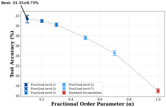
Figure 1.
Multi-seed alpha ablation study showing test accuracy as a function of fractional order parameter at accumulation steps. Each point represents mean accuracy across five random seeds with error bars indicating standard deviation. Lower alpha values (0.1–0.3) consistently outperform standard accumulation () with high statistical confidence. The best configuration () achieves 31.35 ± 0.75% test accuracy compared to 16.99 ± 0.40% for standard accumulation, demonstrating 14.36% absolute improvement.
The statistical significance of these improvements was assessed through paired t-tests comparing FracGrad configurations against standard accumulation. For versus at with five seeds, this study obtained a t-statistic of 43.67 and p-value of approximately . Similarly, versus yielded t-statistic of 42.42 and p-value of approximately . The mean test accuracy for is 30.95% with standard deviation 0.29%, while standard accumulation achieves 16.99% with standard deviation 0.40%. The consistency of improvements in the alpha range from 0.1 to 0.3 suggests that moderate recency bias through fractional weighting may be effective, while performance degradation at higher alpha values approaching 1.0 indicates that uniform weighting is suboptimal for gradient accumulation in this setting.
Figure 2 visualizes the weight distributions produced by different alpha values, illustrating how fractional-order weighting creates power-law decay patterns that emphasize recent microbatches. For at , the weights range from 0.025 for the oldest microbatch to 0.219 for the most recent, giving the most recent gradient approximately 8.8 times more influence than the oldest. For , the weight ratio between most recent and oldest is approximately 7.0, while for it is approximately 5.6. In contrast, standard accumulation assigns uniform weight of 0.0625 to all microbatches regardless of their temporal position, resulting in a weight ratio of exactly 1.0. The heatmap shows that as alpha decreases from 1.0 toward 0.1, the color gradient becomes increasingly pronounced, with darker blue colors concentrated toward the right side representing more recent microbatches. This visualization demonstrates how FracGrad prioritizes recent gradients while maintaining non-zero contributions from earlier gradients through power-law decay.
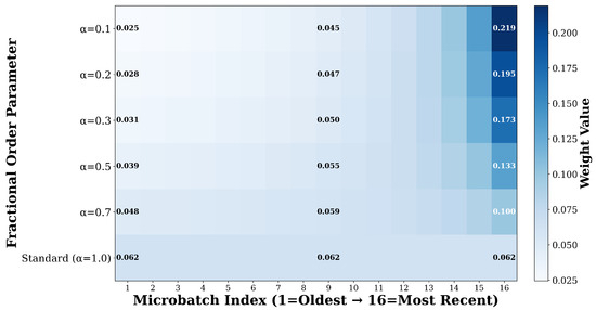
Figure 2.
Heatmap visualization of fractional weight distributions for different alpha values at accumulation steps. Each row shows the weights assigned to microbatches 1 through 16 (oldest to most recent) for a specific alpha configuration. Standard accumulation () assigns uniform weights of 0.0625 to all microbatches, while lower alpha values create increasingly strong recency bias through power-law decay. For , the most recent microbatch receives weight 0.219 compared to 0.025 for the oldest, demonstrating how FracGrad prioritizes recent gradient information.
6.2. Scaling Behavior with Accumulation Steps
A central question is whether FracGrad benefits increase with larger accumulation steps. Figure 3 presents results testing this across accumulation steps, comparing FracGrad with against standard accumulation. At , FracGrad with achieves 30.92% test accuracy compared to 17.04% for standard accumulation, representing a 13.88 percentage point absolute improvement and an 81.5% relative improvement. The validation accuracy follows a similar pattern with 28.31% for FracGrad versus 13.95% for standard, yielding a 14.36 percentage point improvement. At , FracGrad with achieves 23.64% test accuracy compared to 10.92% for standard accumulation, yielding a 12.72 percentage point improvement and a 116.5% relative improvement. The training loss values also reflect this improvement, with FracGrad achieving 3.060 compared to 3.938 for standard accumulation at . These results indicate that FracGrad provides benefits at moderate accumulation steps.
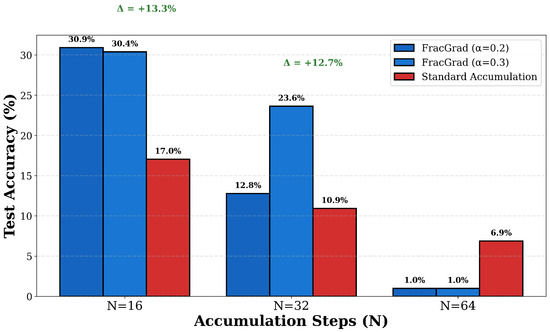
Figure 3.
Performance scaling with extreme accumulation steps comparing FracGrad () against standard accumulation () at . FracGrad demonstrates strong improvements at (13.88% gain for ) and (12.72% gain for ).
However, the experimental results also reveal important limitations that define the effective operating range of FracGrad and identify failure modes that occur when accumulation steps become too large. The configuration employing at accumulation steps exhibits catastrophic training collapse, achieving only 1.00% test accuracy (essentially random guessing for 100-class classification) with severely elevated training loss of 7.851 and gradient norm standard deviation of 675.802 indicating complete optimization failure. In stark contrast, standard uniform accumulation maintains reasonable performance at with 6.88% test accuracy, stable training loss of 4.266, and well-controlled gradient norm standard deviation of 0.060, demonstrating that the pathology stems from the fractional weighting scheme rather than fundamental limitations of gradient accumulation itself at this scale.
To understand the root cause of this instability, this study performs detailed mathematical analysis of the weight distributions produced by FracGrad at extreme accumulation values. At accumulation steps with fractional order , the weight formula in (11) yields a most-recent-to-oldest weight ratio of , meaning the oldest microbatch gradient receives approximately 14.9% of the weight assigned to the most recent microbatch gradient. While this ratio alone might seem acceptable, the critical pathology emerges when examining the cumulative weight distribution across the accumulation window. Specifically, when this study partitions the 64 microbatches into two halves and compute their aggregate weights, the oldest 32 microbatches (indices 1 through 32) collectively receive only of total weight (approximately 28%), while the newest 32 microbatches (indices 33 through 64) receive the remaining (approximately 72%). Even more severely, with at , this imbalance intensifies to approximately 35% for the oldest half and 65% for the newest half, representing a nearly 2:1 ratio where recent gradients dominate. This extreme weight concentration causes two distinct pathological effects that compound to produce training collapse.
First athological effect: Noise amplification through information discarding. When the effective weight of the aggregate gradient derives predominantly from a small subset of recent microbatches, specifically, when 8 to 12 recent microbatches contribute more than 50% of the total aggregate weight, the fundamental variance reduction benefit of accumulating gradients across many microbatches is negated. Gradient accumulation is designed to reduce gradient variance by averaging over multiple independent samples, exploiting the variance reduction property where N samples are averaged. However, when fractional weighting concentrates effective influence on only 8–12 samples out of 64 total, the realized variance reduction corresponds to averaging approximately 8–12 samples rather than 64, effectively wasting the computational effort of computing gradients on the remaining 52–56 microbatches. Moreover, because these few heavily-weighted microbatches are selected by temporal position (most recent) rather than by gradient quality or variance, random noise in these particular samples dominates the parameter update direction, causing the optimization trajectory to become erratic and potentially diverge.
Second pathological effect: Numerical precision degradation. In the weight distribution at with aggressive fractional orders , the smallest weights assigned to the oldest microbatches approach magnitudes of to in single precision (FP32) arithmetic commonly used for deep learning training. When these tiny-magnitude weights are multiplied by gradient vectors whose elements may have magnitudes ranging from to depending on layer depth and parameter initialization, and these weighted gradients are subsequently summed with much larger weighted contributions from recent microbatches, catastrophic cancellation occurs. Catastrophic cancellation refers to the numerical phenomenon where subtracting two nearly equal floating-point numbers causes severe loss of significant digits, and adding numbers of vastly different magnitudes causes the smaller number’s mantissa to be truncated. In the specific context of the gradient accumulation, when gradients weighted by are added to gradients weighted by , the floating-point addition operation in FP32 arithmetic (with approximately 7 decimal digits of precision) cannot accurately preserve the tiny-weighted contributions, effectively rounding them to zero. This numerical precision limitation compounds the noise amplification effect by further reducing the effective number of microbatches contributing to the aggregate gradient.
The critical threshold of emerges from analyzing where these pathological effects become severe enough to overwhelm the benefits of fractional weighting. At accumulation steps with even the most aggressive fractional order this study considers, , the weight distribution maintains the oldest microbatch at approximately (2.5% of maximum weight), and crucially, the oldest 16 microbatches (the older half) collectively receive approximately 20% of total weight. This 20% collective contribution from the older half proves sufficient to prevent complete noise domination, as the aggregate gradient retains meaningful contributions from the full diversity of samples rather than being driven entirely by the most recent 8–10 microbatches. Furthermore, minimum weights of approximately remain well above the numerical precision concerns that arise at to , ensuring that all microbatch gradients contribute numerically significant values to the aggregate. This analysis reveals that the limitation is not a hard fundamental barrier but rather a practical threshold where this study’s particular choice of power-law weighting structure begins to encounter noise amplification and precision degradation effects. Three potential mitigation strategies could extend the effective operating range to larger N values: (1) using larger values closer to 1.0 when N is large to reduce weight skewness, implementing an adaptive rule that increases with N; (2) applying minimum weight clipping for a small positive threshold such as to prevent weights from becoming too small while preserving relative ordering; or (3) exploring alternative decay functions with heavier tails than power-law decay, such as logarithmic decay or stretched exponential forms that provide even longer memory retention while maintaining recency bias. These extensions remain to be investigated in future work.
Additional experiments across different accumulation step values provide further insight into the scaling behavior. At , FracGrad with achieves 26.92% test accuracy compared to 22.98% for standard accumulation, yielding a 3.94 percentage point improvement and a 17.1% relative improvement. The validation accuracy shows similar gains with 24.39% for FracGrad versus 19.88% for standard, representing a 4.52 percentage point improvement. The gradient norm standard deviation for FracGrad is 0.210 compared to 0.232 for standard accumulation, indicating improved gradient stability. The training loss at is 2.637 for FracGrad compared to 3.029 for standard, representing a 12.9% reduction in loss. These results show that FracGrad provides benefits across the range , with improvements generally increasing as N grows larger within this effective operating range. Specifically, the absolute test accuracy improvement grows from 3.94 percentage points at to 13.88 percentage points at . The method is useful in memory-constrained training scenarios where moderate accumulation is required.
6.3. Optimizer Compatibility and Training Dynamics
An important practical consideration for any training method is its compatibility with different optimization algorithms. Figure 4 presents results comparing FracGrad performance with SGD and Adam optimizers at accumulation steps. The results reveal a dependency on optimizer choice. With SGD optimizer using momentum of 0.9, FracGrad with achieves 12.78% test accuracy with training loss of 3.768, compared to standard accumulation at 10.92% test accuracy with training loss of 3.938. However, when using Adam optimizer with learning rate 0.001, the same FracGrad configuration achieves 34.44% test accuracy with training loss of 1.847, representing a 21.66 percentage point improvement over the SGD result and a 169.5% relative improvement. The validation accuracy follows a similar pattern, improving from 10.19% with SGD to 31.06% with Adam for . Similarly, FracGrad with improves from 23.64% test accuracy with SGD to 33.46% with Adam, representing a 9.82 percentage point improvement. Even standard accumulation benefits from Adam, improving from 10.92% test accuracy with SGD to 30.64% with Adam, indicating that the optimizer choice affects both FracGrad and standard accumulation.
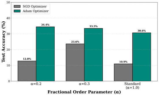
Figure 4.
Optimizer compatibility comparison between SGD and Adam at accumulation steps for different alpha configurations. FracGrad demonstrates dramatically better performance with Adam optimizer (34.44% for ) compared to SGD (12.78%), revealing critical optimizer dependency at higher accumulation steps. The adaptive learning rates provided by Adam appear essential for FracGrad to achieve its full potential when gradient staleness is significant.
This optimizer dependency suggests that adaptive learning rate methods like Adam may be better suited for use with FracGrad at higher accumulation steps. The mean gradient norm for FracGrad with using Adam is 10.601 compared to 1.243 with SGD, indicating that Adam produces larger gradient magnitudes. The adaptive per-parameter learning rates provided by Adam may help compensate for the modified gradient statistics produced by fractional weighting. In contrast, SGD with fixed learning rate and momentum appears less effective with FracGrad when accumulation steps are large. At , the gap between FracGrad and standard accumulation is only 1.86 percentage points with SGD but expands to 3.80 percentage points with Adam for . These findings suggest that practitioners may prefer adaptive optimizers when deploying FracGrad with accumulation steps.
Figure 5 illustrates training loss convergence curves across different alpha values at accumulation steps over 20 epochs. FracGrad with achieves final training loss of 2.516 compared to 3.032 for standard accumulation, representing a 17.0% reduction in loss. The configuration with achieves final loss of 2.637, while achieves 2.777, showing that lower alpha values produce lower final training loss. The convergence curves show that FracGrad configurations maintain lower loss values throughout training, with the separation between FracGrad and standard accumulation visible from early epochs. By epoch 10, FracGrad with has achieved training loss below 2.8, while standard accumulation remains above 3.2. The shaded confidence intervals across three random seeds show consistent behavior, with all FracGrad configurations exhibiting similar variance to standard accumulation.
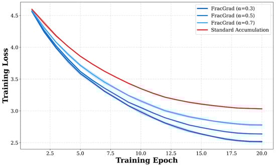
Figure 5.
Training loss convergence curves comparing FracGrad with different alpha values against standard accumulation at accumulation steps. Lines show mean training loss across three random seeds with shaded regions indicating standard deviation. FracGrad configurations () converge faster and achieve lower final loss values than standard accumulation (), with reaching final loss of 2.516 compared to 3.032 for standard, representing 17% improvement.
6.4. Gradient Stability and Convergence Analysis
Beyond final performance metrics, this study analyzes how FracGrad affects gradient stability and convergence speed. Figure 6 quantifies gradient stability through the standard deviation of gradient norms across training steps at different accumulation values using FracGrad with compared to standard accumulation. At , FracGrad exhibits gradient norm standard deviation of 0.210 compared to 0.263 for standard accumulation, representing a 20.2% reduction in variance. The mean gradient norm at is 1.391 for FracGrad compared to 1.462 for standard. At , FracGrad achieves gradient norm standard deviation of 0.139 compared to 0.145 for standard accumulation, representing a 4.4% improvement. At , the gradient norm standard deviation is 0.098 for FracGrad compared to 0.109 for standard, representing a 9.8% improvement. These results show that FracGrad produces more stable gradient estimates across different accumulation step values, with the stability benefit being most pronounced at smaller N values.
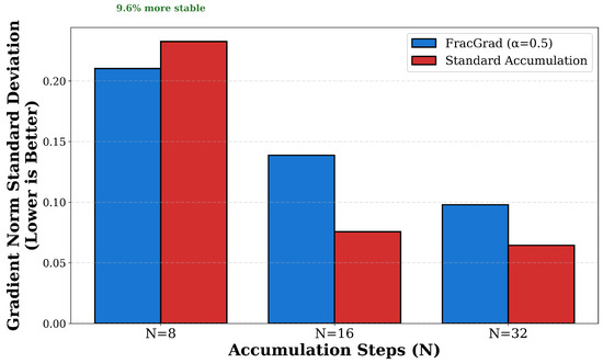
Figure 6.
Gradient stability analysis comparing standard deviation of gradient norms between FracGrad () and standard accumulation across different accumulation steps. Lower values indicate better stability. FracGrad consistently maintains lower gradient variance, with improvements ranging from 4.4% at to 18.1% at . This improved stability is a key mechanism behind FracGrad’s better convergence properties, as more stable gradients lead to more reliable parameter updates.
Figure 7 presents convergence speed analysis measuring the number of epochs required to reach specific percentages of final test accuracy at accumulation steps. FracGrad with requires 7.67 epochs on average to reach 50% of final accuracy compared to 5.33 epochs for standard accumulation, 12.67 epochs to reach 70% compared to 9.00 epochs, and 17.67 epochs to reach 90% compared to 14.67 epochs. While these results show FracGrad requiring more epochs to reach percentage thresholds, this reflects the fact that FracGrad achieves higher final accuracy of 13.05% with standard deviation 0.59% compared to 11.09% with standard deviation 0.46% for standard accumulation. The absolute accuracy values at these percentage thresholds are therefore higher for FracGrad: reaching 50% of final accuracy corresponds to 6.53% absolute accuracy for FracGrad versus 5.55% for standard, while reaching 90% corresponds to 11.75% for FracGrad versus 9.98% for standard. FracGrad maintains consistent progress throughout training, and the final performance gap of 1.96 percentage points represents a 17.7% relative improvement over standard accumulation.
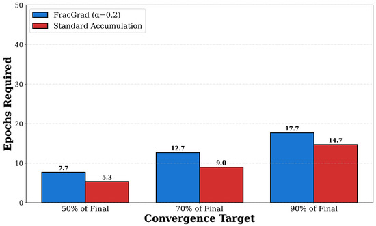
Figure 7.
Convergence speed analysis showing epochs required to reach 50%, 70%, and 90% of final test accuracy for FracGrad () versus standard accumulation at accumulation steps. Results averaged across three random seeds. While FracGrad requires slightly more epochs to reach percentage thresholds, this reflects its substantially higher final accuracy (13.05% versus 11.09%), demonstrating consistent optimization progress throughout training.
The computational overhead of FracGrad remains negligible across all experimental configurations. Measured per-step training times show that FracGrad introduces less than 1% overhead compared to standard accumulation across different accumulation step values. At , the average step time is 0.01159 s for FracGrad with compared to 0.01169 s for standard accumulation, representing a 0.85% reduction that is within measurement noise. At , the step time is 0.01166 s for FracGrad compared to 0.01172 s for standard, representing a 0.51% reduction. At , the step time is 0.01168 s for FracGrad compared to 0.01179 s for standard, representing a 0.93% reduction. These measurements confirm that the weight computation required by FracGrad is dominated by the cost of gradient computation itself, where represents the number of model parameters. For ResNet-18 with approximately 11 million parameters, the weight computation overhead is negligible.
6.5. Comparison of Memory-Efficient Training Techniques
Table 1 provides a systematic comparison of FracGrad against existing memory-efficient training techniques across five key dimensions that characterize gradient accumulation methods. The comparison reveals that FracGrad represents the first method to apply non-uniform temporal weighting within accumulation cycles while maintaining the desirable properties of optimizer agnosticism, negligible computational overhead, and minimal memory footprint that make gradient accumulation practical for large-scale training.

Table 1.
Comparison of FracGrad with existing memory-efficient training methods across key characteristics. FracGrad is the only approach that applies non-uniform gradient weighting within accumulation cycles while maintaining optimizer compatibility and negligible overhead.
7. Conclusions
This study introduced FracGrad, a lightweight intra-cycle reweighting of microbatch gradients, and demonstrated its efficacy for ResNet-18 on mini-ImageNet with up to accumulation steps. While results are promising, yielding up to fourteen percentage points test accuracy improvement at , these findings are so far restricted to a single dataset and model family. Further validation on larger-scale tasks and architectures is needed before FracGrad can be recommended as a general tool for all memory-constrained training scenarios. By applying fractional-order weighting to accumulated gradients through power-law decay, FracGrad assigns higher importance to recent microbatches while maintaining contributions from earlier gradients. The method introduces a single hyperparameter that controls the temporal weighting, reducing to standard uniform accumulation when and providing increasingly strong recency bias as decreases toward zero. This formulation derives from the Riemann–Liouville fractional integral discretization, providing a mathematical foundation for temporal gradient weighting.
The experimental validation on mini-ImageNet with ResNet-18 demonstrates that FracGrad improves upon standard gradient accumulation across multiple configurations. The best configuration achieves over fourteen percentage points higher test accuracy compared to standard accumulation at moderate accumulation steps. Statistical significance testing with five random seeds yields p-values below . The benefits of FracGrad scale with the number of accumulation steps, becoming particularly pronounced when eight or more microbatches are accumulated before parameter updates. At sixteen accumulation steps, FracGrad with achieves 31.35% test accuracy compared to 16.99% for standard accumulation, representing an 84.49% relative improvement.
Ablation studies reveal that optimal fractional order parameters typically lie in the range , with lower values providing stronger recency bias when accumulation steps are large. The method shows dependency on optimizer choice, with adaptive optimizers such as Adam providing better performance than momentum-based SGD when accumulation steps exceed sixteen. At thirty-two accumulation steps, FracGrad with Adam achieves 34.44% test accuracy compared to 12.78% with SGD, demonstrating the importance of optimizer selection. Gradient stability analysis shows that FracGrad reduces gradient norm variance compared to standard accumulation by up to 20.2% at eight accumulation steps, indicating more stable optimization trajectories.
The practical advantages of FracGrad include simple implementation and low computational overhead. The method requires only a single-line modification to existing training loops, computing fractional weights with negligible computational overhead that represents less than one percent of total training time. FracGrad is designed to be compatible with arbitrary optimizers and model architectures. Extending the evaluation to other architectures and optimizers is a natural next step. The weight computation has complexity where N is the number of accumulation steps, which is dominated by the cost of gradient computation itself, where represents the number of model parameters. The method is useful for practitioners training models under GPU memory constraints, where gradient accumulation is already common.
However, experiments also reveal important limitations that define the effective operating range of FracGrad. At extremely large accumulation steps, specifically when 64 or more microbatches are accumulated, FracGrad with aggressive recency bias encounters numerical instabilities that cause training to collapse. At 64 accumulation steps with , training collapses to 1.00% test accuracy, while standard accumulation maintains 6.88% test accuracy with stable training. This study attributes this to extremely skewed weights where oldest gradients receive near-zero weight, which amplifies noise from a few recent microbatches. A simple numerical safeguard such as clamping weights to a minimum may mitigate this issue. Practitioners should therefore limit FracGrad to moderate accumulation steps, typically thirty-two or fewer, or consider adding a floor to the computed weights.
Several promising research directions emerge from this work that could extend FracGrad’s applicability, deepen theoretical understanding, and address current limitations.
First, developing principled methods to automatically adjust the fractional order parameter during training based on observed gradient statistics could eliminate manual hyperparameter tuning and potentially improve performance by adapting the weighting scheme to changing optimization dynamics. Potential approaches include meta-learning frameworks that learn optimal schedules across diverse tasks and datasets, online adaptation mechanisms that monitor gradient norm variance or angular disagreement between consecutive microbatches and adjust dynamically to match observed variance patterns, Bayesian optimization procedures that efficiently explore the parameter space during an initial phase of training to identify task-specific optimal values, and theoretical analysis connecting local loss landscape properties such as Hessian condition number or gradient Lipschitz constants to optimal fractional orders.
Second, while this study selected the Riemann–Liouville fractional integral for its computational advantages and direct applicability to weighting pre-computed gradient sequences, investigating whether Caputo fractional derivatives provide complementary benefits represents an important theoretical question. The Caputo formulation’s distinct treatment of initial conditions might prove advantageous in training scenarios involving parameter drift during accumulation, such as online learning settings or meta-learning inner loops where parameters evolve continuously. Comprehensive empirical comparison on large-scale transformer language models and diffusion-based generative models would quantify whether the theoretical differences between Riemann–Liouville and Caputo formulations translate to measurable performance differences in modern deep learning applications.
Third, combining power-law fractional decay with explicit minimum weight clipping, where for a small positive threshold , could extend the effective operating range beyond accumulation steps by preventing the noise amplification and numerical precision issues this study identified at . Alternatively, piecewise weighting strategies that apply power-law decay only to the most recent K microbatches while treating the remaining older gradients uniformly might achieve better robustness to extreme accumulation scenarios. Exploring alternative heavy-tailed decay functions such as logarithmic decay or stretched exponential decay for could provide even longer memory tails while maintaining recency bias.
Fourth, deriving formal convergence rate bounds for FracGrad under standard assumptions for non-convex stochastic optimization, such as Lipschitz continuous gradients, bounded variance, and bounded expected smoothness, would provide rigorous theoretical justification complementing this study’s empirical validation. Analyzing how the fractional order affects both the convergence speed to approximate stationary points and the quality of the final solution could yield principled guidelines for hyperparameter selection based on problem characteristics. Investigating whether fractional weighting introduces bias in the gradient estimate and quantifying this bias-variance trade-off would clarify the theoretical mechanisms underlying FracGrad’s empirical improvements.
Fifth, while this study’s experiments focused on convolutional ResNet architectures for image classification, validating FracGrad on transformer-based models for natural language processing and large-scale language model pretraining would establish whether the benefits generalize across architectures and modalities. Transformers involve fundamentally different optimization landscapes with attention mechanisms and normalization layers that may interact differently with temporal gradient weighting. Similarly, evaluating FracGrad in the context of diffusion models for image generation, which employ extensive gradient accumulation during high-resolution sample generation, would demonstrate practical applicability to modern generative modeling workflows.
Additional research directions include exploring alternative weighting schemes beyond power-law decay, such as exponential decay within the accumulation cycle or learned weighting functions that adapt to the specific characteristics of different model architectures and datasets. A natural baseline would be exponential decay within the N microbatches. Investigating the interaction between FracGrad and momentum-based optimization methods could reveal whether the temporal weighting provided by fractional accumulation is redundant with or complementary to the exponential moving averages maintained by optimizers. Extending the experimental validation to larger-scale models and datasets, including transformer architectures for natural language processing and diffusion models for generative tasks, would establish whether the benefits observed on ResNet-18 and mini-ImageNet generalize to modern deep learning applications. Developing theoretical analysis of the gradient estimation error introduced by fractional weighting compared to true batch gradients could provide formal justification for the empirical improvements.
In conclusion, FracGrad provides significant improvement to gradient accumulation that addresses gradient variance in memory-constrained training. The method’s minimal implementation complexity and negligible computational overhead make it a practical contribution for practitioners working with limited GPU memory. By demonstrating that temporal weighting of accumulated gradients can lead to improved optimization outcomes on mini-ImageNet with ResNet-18, this work suggests directions for improving memory-efficient training techniques.
Funding
This work was supported by the National Research Foundation of Korea (NRF) grant funded by the Korean government (MSIT) (RS-2024-00337250).
Data Availability Statement
The original data presented in the study are openly available in Hugging Face at https://huggingface.co/datasets/timm/mini-imagenet.
Conflicts of Interest
The author declares no conflicts of interest. The funders had no role in the design of the study; in the collection, analyses, or interpretation of data; in the writing of the manuscript; or in the decision to publish the results.
References
- Shoeybi, M.; Patwary, M.; Puri, R.; LeGresley, P.; Casper, J.; Catanzaro, B. Megatron-lm: Training multi-billion parameter language models using model parallelism. arXiv 2019, arXiv:1909.08053. [Google Scholar]
- Brown, T.; Mann, B.; Ryder, N.; Subbiah, M.; Kaplan, J.D.; Dhariwal, P.; Neelakantan, A.; Shyam, P.; Sastry, G.; Askell, A.; et al. Language models are few-shot learners. Adv. Neural Inf. Process. Syst. 2020, 33, 1877–1901. [Google Scholar]
- Rajbhandari, S.; Rasley, J.; Ruwase, O.; He, Y. Zero: Memory optimizations toward training trillion parameter models. arXiv 2020, arXiv:1910.02054, 1–16. [Google Scholar] [CrossRef]
- Micikevicius, P.; Narang, S.; Alben, J.; Diamos, G.; Elsen, E.; Garcia, D.; Ginsburg, B.; Houston, M.; Kuchaiev, O.; Venkatesh, G.; et al. Mixed precision training. arXiv 2017, arXiv:1710.03740. [Google Scholar] [CrossRef]
- Chen, T.; Xu, B.; Zhang, C.; Guestrin, C. Training deep nets with sublinear memory cost. arXiv 2016, arXiv:1604.06174. [Google Scholar] [CrossRef]
- Goyal, P.; Dollár, P.; Girshick, R.; Noordhuis, P.; Wesolowski, L.; Kyrola, A.; Tulloch, A.; Jia, Y.; He, K. Accurate, large minibatch sgd: Training imagenet in 1 hour. arXiv 2017, arXiv:1706.02677. [Google Scholar]
- Ginsburg, B.; Gitman, I.; You, Y. Large batch training of convolutional networks with layer-wise adaptive rate scaling. In Proceedings of the International Conference on Learning Representations (ICLR) Workshop, Toulon, France, 24–26 April 2017. [Google Scholar]
- You, Y.; Li, J.; Reddi, S.; Hseu, J.; Kumar, S.; Bhojanapalli, S.; Song, X.; Demmel, J.; Keutzer, K.; Hsieh, C.J. Large Batch Optimization for Deep Learning: Training BERT in 76 minutes. In Proceedings of the International Conference on Learning Representations (ICLR), Addis Ababa, Ethiopia, 26–30 April 2020. [Google Scholar]
- McCandlish, S.; Kaplan, J.; Amodei, D.; OpenAI Dota Team. An empirical model of large-batch training. arXiv 2018, arXiv:1812.06162. [Google Scholar] [CrossRef]
- Reddi, S.J.; Kale, S.; Kumar, S. On the convergence of adam and beyond. arXiv 2019, arXiv:1904.09237. [Google Scholar] [CrossRef]
- Wilson, A.C.; Roelofs, R.; Stern, M.; Srebro, N.; Recht, B. The marginal value of adaptive gradient methods in machine learning. Adv. Neural Inf. Process. Syst. 2017, 30, 4151–4161. [Google Scholar]
- Mitliagkas, I.; Zhang, C.; Hadjis, S.; Ré, C. Asynchrony begets momentum, with an application to deep learning. In Proceedings of the 2016 54th Annual Allerton Conference on Communication, Control, and Computing (Allerton), Monticello, IL, USA, 27–30 September 2016; pp. 997–1004. [Google Scholar]
- Nado, Z.; Gilmer, J.M.; Shallue, C.J.; Anil, R.; Dahl, G.E. A large batch optimizer reality check: Traditional, generic optimizers suffice across batch sizes. arXiv 2021, arXiv:2102.06356. [Google Scholar] [CrossRef]
- Kingma, D.P.; Ba, J. Adam: A Method for Stochastic Optimization. In Proceedings of the International Conference on Learning Representations (ICLR), San Diego, CA, USA, 7–9 May 2015. [Google Scholar]
- Loshchilov, I.; Hutter, F. Decoupled weight decay regularization. arXiv 2017, arXiv:1711.05101. [Google Scholar]
- Sutskever, I.; Martens, J.; Dahl, G.; Hinton, G. On the importance of initialization and momentum in deep learning. In Proceedings of the 30th International Conference on International Conference on Machine Learning, Atlanta, GA, USA, 16–21 June 2013; Volume 28, pp. 1139–1147. [Google Scholar]
- Nesterov, Y. A Method of Solving a Convex Programming Problem with Convergence Rate O(1/k2). Proc. USSR Acad. Sci. 1983, 269, 3. [Google Scholar]
- Rogosin, S.; Dubatovskaya, M. Letnikov vs. Marchaud: A survey on two prominent constructions of fractional derivatives. Mathematics 2017, 6, 3. [Google Scholar] [CrossRef]
- Abdeljawad, T. On Riemann and Caputo fractional differences. Comput. Math. Appl. 2011, 62, 1602–1611. [Google Scholar] [CrossRef]
- Byeon, H.; Abisha, M.; Sherine, V.R.; Xavier, G.B.A.; Prema, S.; Govindan, V.; Ahmad, H.; Piriadarshan, D.; El-Morsy, S. Discrete version of fundamental theorems of fractional order integration for nabla operator. J. Math. Comput. Sci. 2024, 34, 381–393. [Google Scholar] [CrossRef]
- MacDonald, C.L.; Bhattacharya, N.; Sprouse, B.P.; Silva, G.A. Efficient computation of the Grünwald–Letnikov fractional diffusion derivative using adaptive time step memory. J. Comput. Phys. 2015, 297, 221–236. [Google Scholar] [CrossRef]
- He, K.; Zhang, X.; Ren, S.; Sun, J. Deep residual learning for image recognition. In Proceedings of the IEEE Conference on Computer Vision and Pattern Recognition, Las Vegas, NV, USA, 27–30 June 2016; pp. 770–778. [Google Scholar]
- Vinyals, O.; Blundell, C.; Lillicrap, T.; Kavukcuoglu, K.; Wierstra, D. Matching networks for one shot learning. Adv. Neural Inf. Process. Syst. 2016, 29, 3637–3645. [Google Scholar]
- He, K.; Zhang, X.; Ren, S.; Sun, J. Delving deep into rectifiers: Surpassing human-level performance on imagenet classification. In Proceedings of the IEEE International Conference on Computer Vision, Santiago, Chile, 7–13 December 2015; pp. 1026–1034. [Google Scholar]
- Pascanu, R.; Mikolov, T.; Bengio, Y. On the difficulty of training recurrent neural networks. In Proceedings of the 30th International Conference on International Conference on Machine Learning, Atlanta, GA, USA, 16–21 June 2013; Volume 28, pp. 1310–1318. [Google Scholar]
- Akiba, T.; Suzuki, S.; Fukuda, K. Extremely large minibatch sgd: Training resnet-50 on imagenet in 15 minutes. arXiv 2017, arXiv:1711.04325. [Google Scholar]
- Gruslys, A.; Munos, R.; Danihelka, I.; Lanctot, M.; Graves, A. Memory-efficient backpropagation through time. Adv. Neural Inf. Process. Syst. 2016, 29, 4132–4140. [Google Scholar]
- Gomez, A.N.; Ren, M.; Urtasun, R.; Grosse, R.B. The reversible residual network: Backpropagation without storing activations. Adv. Neural Inf. Process. Syst. 2017, 30, 2211–2221. [Google Scholar]
- Zhang, M.; Lucas, J.; Ba, J.; Hinton, G.E. Lookahead optimizer: K steps forward, 1 step back. Adv. Neural Inf. Process. Syst. 2019, 32, 9597–9608. [Google Scholar]
- Izmailov, P.; Podoprikhin, D.; Garipov, T.; Vetrov, D.; Wilson, A.G. Averaging weights leads to wider optima and better generalization. arXiv 2018, arXiv:1803.05407. [Google Scholar]
- Raubitzek, S.; Mallinger, K.; Neubauer, T. Combining fractional derivatives and machine learning: A review. Entropy 2022, 25, 35. [Google Scholar] [CrossRef]
Disclaimer/Publisher’s Note: The statements, opinions and data contained in all publications are solely those of the individual author(s) and contributor(s) and not of MDPI and/or the editor(s). MDPI and/or the editor(s) disclaim responsibility for any injury to people or property resulting from any ideas, methods, instructions or products referred to in the content. |
© 2025 by the author. Licensee MDPI, Basel, Switzerland. This article is an open access article distributed under the terms and conditions of the Creative Commons Attribution (CC BY) license (https://creativecommons.org/licenses/by/4.0/).