Abstract
Fractional differential equations offer a natural framework for describing systems in which present states are influenced by the past. This work presents a nonlinear Caputo-type fractional differential equation (FDE) with a nonlocal initial condition and attempts to describe a model of memory-dependent behavioral adaptation. The proposed framework uses a fractional-order derivative to discuss the long-term memory effects. The existence and uniqueness of solutions are demonstrated by Banach’s and Krasnoselskii’s fixed-point theorems. Stability is analyzed through Ulam–Hyers and Ulam–Hyers–Rassias benchmarks, supported by sensitivity results on the kernel structure and fractional order. The model is further employed for behavioral despair and learned helplessness, capturing the role of delayed stimulus feedback in shaping cognitive adaptation. Numerical simulations based on the convolution-based fractional linear multistep (FVI–CQ) and Adams–Bashforth–Moulton (ABM) schemes confirm convergence and accuracy. The proposed setup provides a compact computational and mathematical paradigm for analyzing systems characterized by nonlocal feedback and persistent memory.
Keywords:
fractional differential equations; fixed point theory; memory-dependent dynamics; behavioral modeling; Ulam–Hyers stability MSC:
26A33; 34A08; 47H10; 34D20
1. Introduction
Differential equations are used to define the association between a variable and its rate of change. They are a background system of modeling dynamic systems in natural and applied science (see [1,2]). In their most common form, ordinary differential equations (ODEs) involve functions of a single variable and its derivatives. The solution to a differential equation is a function that satisfies the specified relationship between the dependent variable and its derivatives. Researchers apply this framework across physics, biology, and engineering disciplines to model evolving system behavior (for more details, see [3,4,5]).
In behavioral neuroscience, ODEs are commonly used to model learning and memory processes. For instance, the model presented in [6,7] quantifies shock-response rates in animals exposed to aversive stimuli. This model does not consider complex behaviors, such as maze navigation, but instead focuses on the fundamental responses triggered by repeated shocks. The underlying dynamics are expressed by the following integro-differential equation
where is the shock response rate at time t, is a sensitivity parameter, and is a memory kernel that weights the effect of previous shocks. The cumulative influence of past experiences in the process is a part of the integral term, which is the model of memory-dependent changes in behavior. Data used to determine the effect of shock exposure were collected in two animal groups, an experimental group and a control group which was not exposed to shocks (see [8]). Figure 1 and Figure 2 below depict the cumulative number of shocks received by selected animals in the respective groups in the course of time.
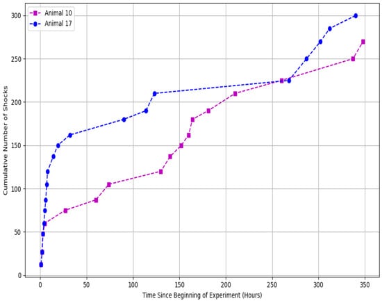
Figure 1.
Cumulative number of shocks in experimental group.
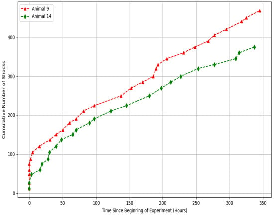
Figure 2.
Cumulative number of shocks in control group.
It has been empirically suggested that the retention of memory decays exponentially over time [9,10]. Hence, a suitable choice for the memory kernel is , where represents a characteristic memory timescale. With this exponential kernel, Equation (1) becomes
In Equation (2), the initial derivative characterizes the animal’s initial reactivity to shocks, while the integral term incorporates the cumulative, decaying influence of past shocks on subsequent behavior.
Nevertheless, the ODE model presumes instant or rapidly decaying memory effects even though memory impacts on behavior can be behavioral dependencies in the long run (for more details, see [11,12]). This is common in neuroscience experimental observations that suggest more complex memory dynamics [13], where past experiences influence future behavior through non-local temporal interactions. Fractional-order differential equations (FDEs) are more useful when such long-term or non-exponential memory processes are involved (see [14,15,16,17]).
Motivated by the limitations of classical ODEs in modeling long-term memory, we propose the following fractional-order model
with initial conditions
In the above system (3)–(4),
- denotes the Caputo fractional derivative of order , which captures memory effects over extended periods;
- represents the behavioral response (e.g., cumulative shocks or response intensity) measured during the experiment;
- is a time-dependent sensitivity parameter controlling the strength of past experiences;
- describes the animal’s behavioral adaptation or reaction to prior stimuli;
- determines how past responses at time influence current behavior at time t.
This study examines a nonlinear memory-dependent system described by a Caputo-type fractional differential equation with a nonlocal initial condition. The model uses a fractional derivative of order to represent long-term memory in behavioral learning under delayed feedback conditions. The existence and uniqueness of solutions are proved using Banach’s contraction principle and Krasnoselskii’s fixed-point theorem. A contractive framework is established with explicit stability conditions based on the fractional order and kernel properties. Numerical solutions are obtained using the Adams–Bashforth–Moulton method [18] and a convolution-based fractional integrator [19].
The paper is structured as follows. Section 2 provides the necessary mathematical preliminaries and notational norms, whereas Section 3 employs fixed-point theorems to establish the existence and uniqueness of solutions under suitable contractivity conditions. Section 4 is dedicated to the discussion of well-posedness, the derivation of the conditions in which the operator is stable. In Section 5, we discuss the sensitivity analysis of the proposed framework. The model is applied to behavioral learning in the use of numerical simulations and comparisons (Section 6). Lastly, Section 7 provides the conclusion and suggests the possible future directions of work.
2. Preliminaries
This section presents key ideas and foundational results employed in the following analysis.
Definition 1
([20]). Let and let be such that . Assume that . The Caputo fractional derivative of order α of the function g is defined by
where denotes the Gamma function and is the m-th derivative of g. The (left-sided) Riemann–Liouville fractional integral of order is given by
The Caputo derivative and Riemann–Liouville integral satisfy the following fundamental identities:
Moreover, the general solution of the homogeneous fractional differential equation
is a polynomial of degree of the form
where are arbitrary constants for .
In classical differential Equations (1) and (2), the term often represents the initial rate of change and can be used as an initial condition. However, for Caputo fractional derivatives of order , such classical derivatives are generally undefined at the initial time . Therefore, the model (3) adopts a parameter in place of , which captures the system’s initial tendency or responsiveness without violating the regularity assumptions required by the Caputo derivative. This substitution ensures the formulation remains mathematically consistent while preserving the interpretability of the model in behavioral terms.
We now prove a lemma necessary for the analysis carried out in later sections.
Lemma 1.
Let and satisfy
where denotes the Caputo fractional derivative of order and is a given constant. Here, is a continuous weighting function, is a continuous nonlinear response function, and is a continuous memory kernel describing the effect of past states. Then z satisfies (9) if and only if it fulfills the following integral equation:
Proof.
Assume first that satisfies (9). Applying the fractional integral operator to both sides of the differential equation gives
Using the standard identity for the Caputo derivative of order for ,
we obtain
Since acts linearly and , the first integral on the right-hand side yields
Hence,
Writing out the fractional integral explicitly gives
Substituting this expression back into the previous equation yields (10).
In our analysis, we will employ the following classical fixed-point results.
Theorem 1
(Banach’s contraction principle [21]). Let be a complete metric space and consider an operator satisfying the contraction condition
where . Then, the operator has a unique fixed point . Moreover, for any initial guess , the iterative sequence converges to , specifically,
Theorem 2
(Krasnoselskii’s fixed-point theorem [22]). Let be a nonempty, bounded, convex, and closed subset of a Banach space . Suppose that operators satisfy the conditions:
- 1.
- , for all ;
- 2.
- is continuous and compact;
- 3.
- is a contraction operator.
Then the operator admits at least one fixed point in the set .
3. Analytical Investigation
To establish the well-posedness of solutions for the integral Equation (10) associated with the fractional differential Equation (9), we construct a functional framework consistent with both the operator’s structure and the required regularity of solutions. We consider the Banach space
equipped with the norm
We impose the following assumptions to ensure the validity of our analysis:
- (A1)
- The sensitivity function is continuous and bounded. Hence, it is uniformly continuous on and satisfies
- (A2)
- The nonlinear function is globally Lipschitz-continuous with constant ; that is,Consequently, f is continuous and bounded on every bounded subset of .
- (A3)
- The memory kernel is continuous on the compact setand measurable in both variables. Therefore, it is bounded, and there exists a constant such that
This framework enables the application of standard fixed-point results, leading directly to our main result.
Theorem 3.
Let be the Banach space equipped with the supremum norm defined in (13), and let be the operator associated with the integral equation
Assume that the conditions (A1)–(A3) hold. Then there exists a constant , explicitly given by
such that, for all ,
Consequently:
- (i)
- If the parameters satisfyi.e., if either the interval length is sufficiently small or the product is suitably bounded, then is a strict contraction on .
- (ii)
- By Banach’s fixed-point theorem, admits a unique fixed point satisfying .
- (iii)
Proof.
We first verify that the operator , defined by (14), is well-defined. Under assumptions (A1)–(A3), the functions , f, and are continuous and bounded, ensuring that for each , the integral operator in (14) is finite and yields a continuous function on the compact interval . Therefore, maps continuous functions into continuous functions, making well-defined.
Next, we establish the contraction property. Let . Then, for each , we have
Using the Lipschitz continuity assumption (A2) for f and the boundedness assumptions (A1) and (A3) for and , respectively, we obtain
Evaluating the integral explicitly, we set , where , so that . Substituting and simplifying, we obtain
The remaining integral equals the Beta function , i.e.,
Hence,
Thus,
Taking the supremum over , we obtain
with the contraction constant given by
By choosing a sufficiently small interval length or suitably restricted parameters , , and , we ensure that . Since is complete with respect to the supremum norm defined in (13), Banach’s fixed-point theorem (Theorem 1) guarantees that the operator possesses a unique fixed point , satisfying .
Remark 1.
It is important to note that the contraction constant depends on the interval length . Since α grows as , we have as . Therefore, Banach’s fixed-point Theorem 1 guarantees a unique solution only on finite intervals for which . For unbounded time domains, the analysis must be carried out locally on successive bounded subintervals of .
Corollary 1.
Under assumptions (A1)–(A3) and the conditions of Theorem 3, the unique solution of the fractional differential Equation (9) depends continuously on the initial condition. Precisely, if and are solutions corresponding to initial conditions and , respectively, then there exists a constant such that
Proof.
Let and denote the solutions of the integral Equation (14) corresponding to initial values and , respectively. Then,
where is the operator defined in (14). Taking the supremum norm on both sides and applying the contraction property of , we obtain
Rearranging terms gives
The result follows by setting , where . □
Theorem 4.
Let be the Banach space equipped with the supremum norm defined in (13). Define operators by
and
Suppose the following conditions hold:
- (H1)
- The operator is continuous and compact on .
- (H2)
- The operator is a contraction on , i.e., there exists a constant such that
- (H3)
- There exists such that for all .
Proof.
Define the operator by
The operator defined by (16) maps each to the fixed function , independent of z. Hence, the image of is a singleton subset of , which is trivially compact and continuous.
The operator defined in (17) satisfies the contraction condition. As shown in Theorem 3, using assumptions (A1)–(A3), we obtain
Therefore, is a contraction with constant
provided is sufficiently small or the parameters are appropriately bounded.
Next, we verify the invariance condition. Let . Then,
Set
To ensure , we choose
Thus, the closed ball is invariant under . By Theorem 4, admits at least one fixed point , satisfying .
Example 1.
Consider the following fractional differential equation (FDE) on the interval with fractional order
subject to the initial condition , where is treated as a model parameter representing the initial response tendency. The model components are specified as follows
These functions satisfy assumptions (A1)–(A3): the functions and are continuous and bounded by 1 on their respective domains, and is Lipschitz-continuous with Lipschitz constant .
The associated integral equation, derived from the Caputo formulation with and , is given by
To verify the contraction condition required by Theorem 3, we compute the constant α using
This yields
Since , Theorem 3 guarantees the existence and uniqueness of a solution to the integral Equation (19) and the associated FDE (18).
We now verify the conditions of Theorem 4. Define the operators
With , , and , we compute
Since with , the invariance condition
is satisfied by choosing .
Hence, the closed ball of radius is invariant under the operator , and all the conditions of Theorem 4 are satisfied. Therefore, both the existence and the uniqueness (via Theorem 4 and Theorem 3) of the solution to the FDE (18) and associated integral Equation (19) are guaranteed.
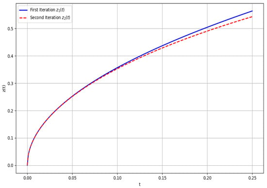
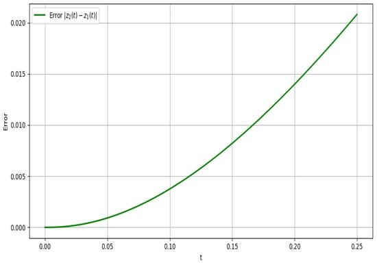
The convergence behavior of the Picard iteration scheme applied to the integral Formulation (19) is illustrated in Figure 3. The first and second iterates, denoted and , are plotted over the interval . The visibly close agreement between the two iterates indicates that the sequence generated by successive applications of the integral operator is rapidly stabilizing. This observation is further corroborated by the error profile in Figure 4, which plots the absolute difference . The error remains small throughout the domain and decays near , demonstrating uniform convergence near the initial condition and verifying that the contraction condition derived analytically is reflected numerically. These figures support the theoretical guarantees of existence, uniqueness, and convergence established via Theorems 3 and 4.
Figure 3.
Convergence of Picard iterations.
Figure 4.
Error between 1st and 2nd iterations.
4. Stability Analysis
In this section, we discuss the stability of the proposed fractional differential equation (FDE) model (3)–(4). For further details on stability, see [23,24,25] and the references cited therein. We begin with the following result.
Theorem 5.
Let be a continuous and integrable function. Suppose is continuously differentiable and satisfies the inequality
where denotes the Caputo derivative of order . Then there exists a unique solution to the integral Equation (10) (and hence to the FDE (9)) such that
where
and is the contraction constant defined in Theorem 3.
Proof.
Let be an approximate solution satisfying the perturbed inequality. Applying the fractional integral operator to both sides of
with , and using the identity , we obtain
Let be the integral operator defined by
Then
Let be the unique fixed point of , guaranteed by Theorem 3, satisfying . So
Taking the supremum norm on both sides gives
Since is a strict contraction with (as established in Theorem 3), the above inequality holds for all . In particular, when (equivalently, ), it reduces to
which implies , and therefore . Hence, the mapping remains strictly contractive even in the unperturbed case, and its unique fixed point x coincides with the exact solution of the proposed fractional model. Hence,
where is defined in (20). This establishes the desired Ulam–Hyers–Rassias stability result. □
Corollary 2.
Proof.
The result follows directly from Theorem 5 by setting for all . □
5. Parameter Sensitivity Analysis
This section analyzes the influence of key parameters on the dynamics of the fractional-order system (3)–(4). Numerical experiments were conducted to study the sensitivity of the solution with respect to the fractional order , the response parameter , the sensitivity function , the initial state , and the stability index .
Figure 5 shows the effect of the memory index on over the interval with . The simulations were performed with using Picard iteration for . The results indicate that smaller values of produce sharper trajectories, reflecting stronger memory effects, while larger values yield smoother and slower responses. These findings demonstrate the central role of in controlling memory depth and temporal adaptation in the model.
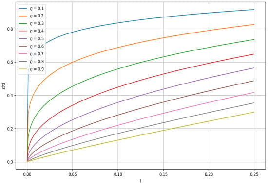
Figure 5.
Sensitivity of the FDE to the fractional order .
Figure 6 depicts the sensitivity of the model to changes in the parameter , which appears linearly in the Caputo integral formulation via the term . As expected, increasing results in uniformly elevated trajectories, reflecting a stronger immediate response to stimuli. The divergence between curves becomes more pronounced over time due to memory retention effects. Thus, serves as a tunable gain factor influencing the early-phase learning or adaptation intensity.
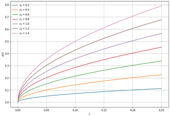
Figure 6.
Sensitivity of the FDE to initial response tendency .
On the other hand, Figure 7 and Figure 8 provide a comparative view of the influence of the time-dependent sensitivity function and the initial state . In Figure 7, we explore five oscillatory forms of , each of which satisfies the boundedness condition . Despite increasing frequency of temporal modulation, the solution curves remain virtually identical over the interval , suggesting that short-term dynamics are predominantly governed by and , rather than by the oscillatory structure of . This robustness under temporal perturbation conditions reinforces the model’s stability in encoding early-time behavioral responses.
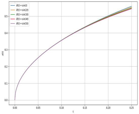
Figure 7.
Sensitivity of the FDE to .
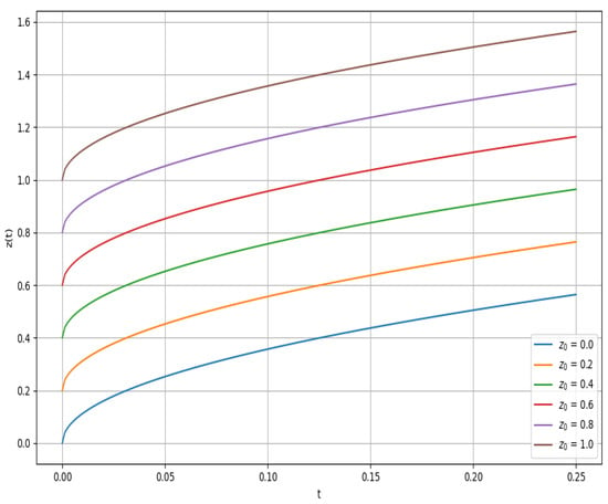
Figure 8.
Sensitivity of the FDE to initial state .
Figure 8 investigates sensitivity to the initial condition , revealing a consistent upward shift in the solution trajectories with increasing , while preserving the overall shape. The nearly parallel evolution of curves indicates that the system responds linearly to perturbations in initial state, confirming well-posedness and stability under initial data variability conditions, in agreement with Corollary 1.
To identify the admissible parameter regimes ensuring well-posedness via Theorem 3, we analyze the stability index defined as
where is the Lipschitz constant of the nonlinearity f, is the supremum norm of the sensitivity function, and bounds the memory kernel . Figure 9 displays a contour plot of over a grid of values. The red dashed curve indicates the critical threshold , demarcating the domain where the integral operator is contractive. The subregion thus characterizes the guaranteed stability zone in which the existence and uniqueness of solutions are ensured. The visualization confirms that model stability is favored by larger values of and shorter observation intervals , consistent with theoretical predictions.
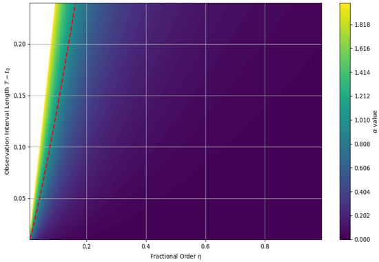
Figure 9.
Stability region for in the plane.
6. Application to Behavioral Despair and Learned Helplessness
We demonstrate the applicability of the proposed fractional-order model (3)–(4) within the learned helplessness paradigm, a classical framework for modeling depressive-like behavior in response to uncontrollable stress. Repeated exposure to aversive stimuli, such as electric shocks, leads to suppression of escape behavior, even when escape becomes feasible.
We consider the following model
subject to the nonlocal initial condition
The interval corresponds to the duration of the behavioral trial, with denoting the onset of stimulus exposure and T the termination of observation. The function represents the temporal evolution of behavioral passivity. Memory dependence is introduced via the Caputo fractional derivative of order , modeling nonlocal effects of prior responses. The constant reflects a suppressed initial reactivity. The sensitivity function models temporal attenuation of stimulus influence, whereas the nonlinearity is incorporated through , imposing bounded growth of passivity. The memory kernel allows sustained influence of past events through power-law decay. The integral-type initial condition (22) encodes dependence on anticipated future behavior via exponential discounting. Figure 10 depicts the experimental setting and the feedback mechanisms linking aversive input, accumulated memory, and behavioral output.
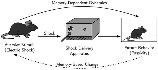
Figure 10.
Schematic representation of the learned helplessness experiment and memory-dependent behavioral adaptation.
We now verify that model (21)–(22) satisfies all analytical conditions for well-posedness and stability on the interval . The sensitivity function is continuous and satisfies . The nonlinearity is globally Lipschitz with constant , and the kernel is continuous and bounded by . Thus, assumptions (A1)–(A3) hold.
To evaluate the nonlocal initial condition , we adopt the approximation , which reflects the empirical pattern of behavioral saturation. With , this yields , used for computing the subsequent constants.
The contraction constant is given by
which satisfies the condition of Theorem 3. Hence, the model admits a unique solution.
To verify the existence via Theorem 4, we decompose the operator as
Here, is compact and independent of z, while satisfies the contraction condition with the same constant . The ball with radius is invariant under , ensuring the existence of a solution.
For Ulam–Hyers–Rassias stability (Theorem 5), all hypotheses are satisfied. The resulting stability bound is
Thus, the proposed model is analytically well-posed, admits a unique solution, and is stable under perturbation conditions in the sense of the Ulam–Hyers–Rassias criterion (see Theorem 5).
The analytical properties of the proposed model (21)–(22) results were first examined through the contraction constant , which determines the applicability of Theorem 3. Figure 11 and Figure 12 provide a parametric view of as a function of the interval length and the fractional order , respectively. In Figure 11, it is observed that for each fixed , increases monotonically with the interval length. Beyond a critical length, contractivity fails (), thereby violating the uniqueness condition. This threshold is more restrictive for smaller , indicating that systems with stronger memory effects impose tighter limitations on admissible domains. Figure 12 complements this by fixing several interval lengths and plotting against . Here, a monotonic decrease in is evident, and for each fixed interval, there exists a threshold order above which . These two perspectives jointly delineate a well-defined stability region in the parameter space and offer explicit criteria for selecting model parameters that guarantee analytical well-posedness.
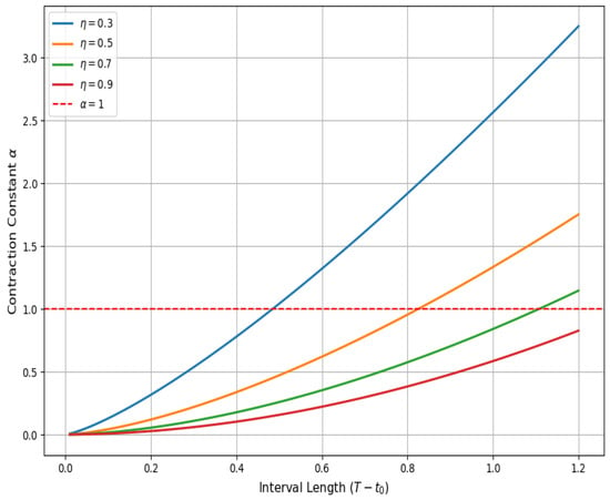
Figure 11.
Contraction constant vs. interval length.
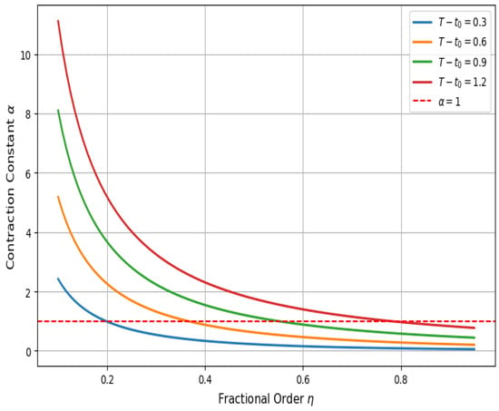
Figure 12.
Contraction constant vs. fractional order.
The dynamical implications of varying the fractional order are illustrated in Figure 13. As decreases, solutions exhibit stronger memory retention, with a sharper initial decline in , followed by a delayed transition to steady behavior. For higher , this behavior progressively shifts toward classical ODE-like decay. This transition is most evident as , where memory effects diminish, and the system responds more immediately to the external stimulus. These trends confirm the capacity of the fractional framework to interpolate between highly nonlocal and memoryless dynamics.
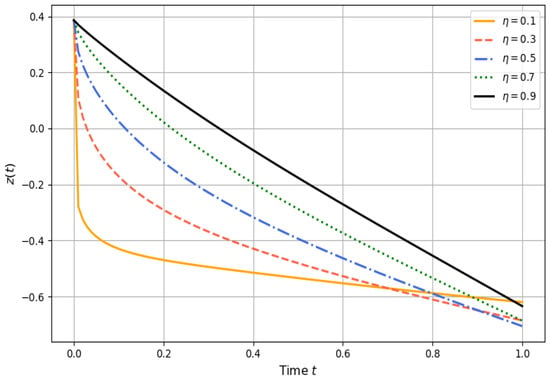
Figure 13.
Effect of fractional order on system trajectory .
To evaluate numerical behavior, the Adams–Bashforth–Moulton method (ABMM) and a fractional variational integrator based on convolution quadrature (FVI–CQ) were applied to the model for . As shown in Figure 14, both schemes produced nearly identical trajectories. The corresponding error curve in Figure 15 shows that the absolute discrepancy remained below over the entire interval, with no signs of numerical instability. These results demonstrate that both methods offer robust numerical approximations, despite their different algorithmic constructions as one based on predictor–corrector discretization and the other on convolution-weighted integration.

Figure 14.
Solution trajectories: ABMM vs. FVI–CQ.
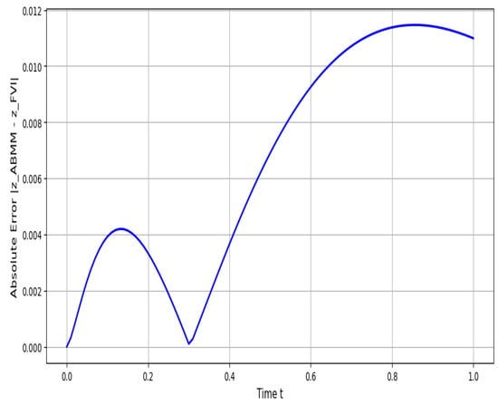
Figure 15.
Absolute error between ABMM and FVI–CQ methods.
Further comparison of numerical accuracy is provided in Figure 16, where both schemes were evaluated with progressively refined step sizes . The maximum error relative to a reference solution was computed for each case. The near-parallel slopes of both error curves in the log–log scale confirm that the methods exhibit similar convergence behavior, with consistent order across refinements. No irregular error growth was observed, reinforcing the numerical stability of both approaches. These results confirm that the FVI–CQ method, despite its heavier formulation, can match the convergence accuracy of the ABMM.
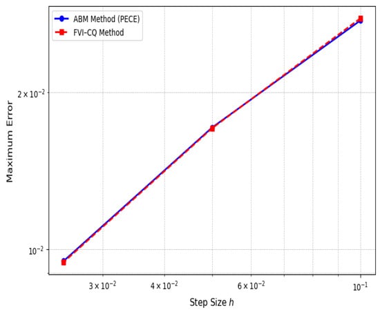
Figure 16.
Convergence of ABMM and FVI–CQ.
Computational efficiency was then assessed via performance benchmarks with varying step sizes. Figure 17 shows that both methods incur increased runtime as , but the growth is more pronounced for FVI–CQ due to its reliance on convolution weights. For coarse discretizations, FVI–CQ performs marginally faster, but beyond , the cost increases steeply. In contrast, the ABMM displays a smoother runtime curve with predictable scaling. This suggests that while both methods are viable, the ABMM is computationally more efficient in the fine-mesh regime and preferable when high-resolution accuracy is required.
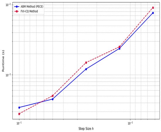
Figure 17.
Runtime comparison across step sizes.
Table 1 delineates the numerical reliability and computational complexity of the two methodologies at various intervals. The results confirm that maximum absolute error remains consistently low, with root mean square error of approximately . Runtime differences are minimal, indicating near-equivalence in computational load per step.

Table 1.
Comparison of ABM and FVI–CQ solutions with maximum absolute error.
The numerical analysis performed using two distinct approximations for the nonlocal term offers insight into the adaptability and robustness of the proposed fractional-order model (21)–(22). Table 2(a) reports the results for the power-law approximation , which enhances long-term memory retention, consistent with fractional dynamics exhibiting strong hereditary effects. The solution trajectories remain closely aligned across both numerical schemes, with the maximum absolute error confined below . The discrepancy peaks near , corresponding to the region of maximal memory influence, after which the solutions converge as , indicating numerical stabilization in the asymptotic regime.
Table 2.
Comparison of ABM and FVI–CQ methods for two approximations of .
In contrast, Table 2(b) presents the corresponding values for the exponential-log approximation , with and . This form induces a rapid saturation of memory, capturing early-time responsiveness followed by a stabilization phase. The numerical outputs remain consistent across solvers, with maximum deviations below , the largest occurring near . This behavior reflects a sharper initial transition governed by the exponential decay, followed by smooth asymptotic alignment.
The convergence patterns illustrated in Figure 18 and Figure 19 reinforce the numerical consistency of both solvers for the two memory profiles. For both approximations, the log–log error curves exhibit a monotonic decline with mesh refinement and no evidence of instability or degradation in accuracy. The close alignment of the curves highlights the inherent numerical stability of the methods. Importantly, the biologically inspired approximation retains convergence behavior comparable to the more singular power-law form. This suggests that the numerical solvers are sufficiently robust to accommodate both strong memory persistence and rapid adaptation, supporting their use in modeling a wide spectrum of memory-dependent cognitive processes.
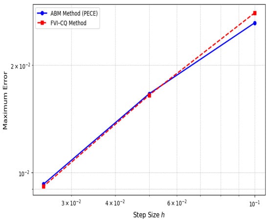
Figure 18.
Convergence under .
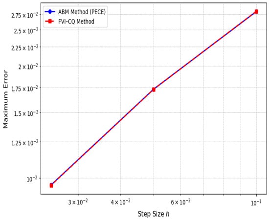
Figure 19.
Convergence under .
To examine the influence of fractional memory strength on system dynamics, we compare numerical solutions of the proposed Caputo-type model (21)–(22) for two fractional orders, and , both selected from within the analytically admissible region determined by contraction-based stability analysis. The approximation is used throughout, representing a biologically plausible learning profile that reflects rapid stimulus-driven adaptation followed by asymptotic saturation. Model parameters are fixed at , , and .
For , the computed well-posedness constants are , contraction constant , bounding constant , with radius and bound . These values indicate that the operator remains weakly contractive, placing the model near the edge of the stable regime. In contrast, at , the values shift to , , , , and , suggesting a significantly stronger contraction and tighter control over solution norms.
The numerical solutions for both regimes are presented in Figure 20 and Figure 21. For , moderate divergence is observed between the two methods in the mid-to-late interval, whereas the curves under are almost indistinguishable. This behavior is quantified in the error profiles (Figure 22 and Figure 23), where the maximum error at reaches , concentrated around , while at , the peak error remains below , an order of magnitude smaller. The smoother and more uniform error decay at higher fractional order reflects the diminished contribution of historical states, consistent with theoretical expectations of reduced memory depth.

Figure 20.
Solution under .
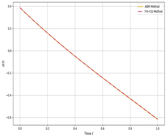
Figure 21.
Solution under .
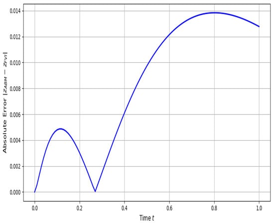
Figure 22.
Error under .

Figure 23.
Error under .
Convergence comparisons (Figure 24 and Figure 25) further corroborate these observations. Both methods exhibit stable and nearly identical convergence behavior across discretizations, but the magnitude of the error decreases significantly for . This improved numerical performance aligns with the analytical contraction results; as , the operator becomes more contractive, and the dynamics progressively resemble classical differential systems.
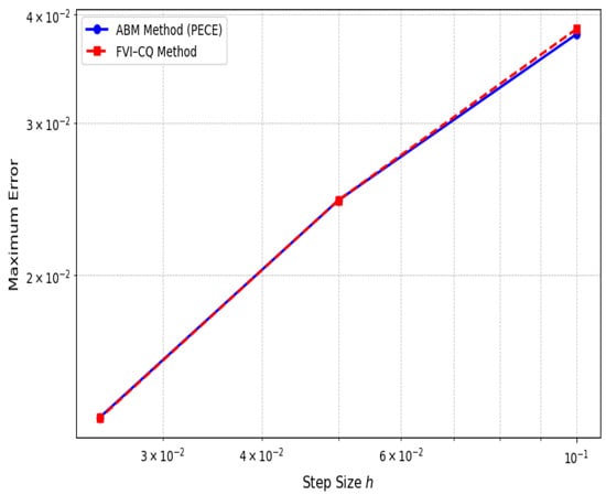
Figure 24.
Convergence under .
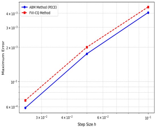
Figure 25.
Convergence under .
7. Conclusions and Open Problems
In this study, we presented a nonlinear Caputo-type fractional differential equation in (3) and (4) to discuss the memory-dependent behavioral adjustment. The existence and uniqueness of solutions were established using Banach’s contraction principle and Krasnoselskii’s fixed-point theorem. The stability analysis determined the permissible parameter range that guarantees the operator’s contractivity. The model was applied to behavioral despair and learned helplessness, demonstrating how feedback delay and memory accumulation shape passivity. Numerical simulations using the Adams–Bashforth–Moulton method and a convolution-based fractional integrator (FVI–CQ) confirmed accuracy and stability across varying fractional orders and memory kernels. Overall, the proposed framework offers a mathematically rigorous and computationally tractable approach for modeling systems with persistent memory and delayed feedback. It provides theoretical and numerical tools for understanding cognitive dynamics in biologically inspired models and can be extended to a broader class of fractional systems exhibiting nonlocality and adaptation.
Several questions remain open for future investigation. An important extension is to examine how stochastic perturbations and random memory kernels influence the long-term stability and convergence of the proposed system. Another promising direction is the development of fractional Lyapunov-based stability criteria and invariant manifold formulations for the nonlinear operator governing the model. A further challenge involves constructing data-driven or neural fractional frameworks capable of estimating both the memory kernel and the fractional order directly from experimental behavioral data.
Author Contributions
Conceptualization, A.T., J.-A.N.-S. and J.-J.T.; Methodology, A.T., W.A., A.M. and J.-J.T.; Validation, A.T., J.-A.N.-S. and A.M.; Formal analysis, J.-A.N.-S. and A.M.; Investigation, J.-A.N.-S., A.M. and J.-J.T.; Resources, W.A.; Data curation, W.A. and J.-J.T.; Writing—original draft and revision, A.T.; Visualization, A.T. and W.A.; Supervision, A.M. and J.-J.T.; Writing—review and editing, A.T. and J.-J.T. All authors have read and agreed to the published version of the manuscript.
Funding
This research is supported by the University of Alicante, Spain; the Spanish Ministry of Science and Innovation; the Generalitat Valenciana, Spain; and the European Regional Development Fund (ERDF) through the following funding sources: At the national level, this work was funded by the following projects: TRIVIAL (PID2021-122263OB-C22) and CORTEX (PID2021-123956OB-I00), granted by MCIN/AEI/10.13039/501100011033 and, as appropriate, co-financed by “ERDF A way of making Europe”, the “European Union”, or the “European Union Next Generation EU/PRTR”. At the regional level, the Generalitat Valenciana (Conselleria d’Educació, Investigació, Cultura i Esport), Spain, provided funding for NL4DISMIS (CIPROM/2021/21).
Data Availability Statement
The original contributions presented in this study are included in the article. Further inquiries can be directed to the corresponding authors.
Conflicts of Interest
The authors state that they do not have any conflicts of interest.
References
- Linot, A.J.; Burby, J.W.; Tang, Q.; Balaprakash, P.; Graham, M.D.; Maulik, R. Stabilized neural ordinary differential equations for long-time forecasting of dynamical systems. J. Comput. Phys. 2023, 474, 111838. [Google Scholar] [CrossRef]
- Turab, A.; Montoyo, A.; Nescolarde-Selva, J.A. Stability and numerical solutions for second-order ordinary differential equations with application in mechanical systems. J. Appl. Math. Comput. 2024, 70, 5103–5128. [Google Scholar] [CrossRef]
- Whitby, M.; Cardelli, L.; Kwiatkowska, M.; Laurenti, L.; Tribastone, M.; Tschaikowski, M. PID control of biochemical reaction networks. IEEE Trans. Autom. Control 2021, 67, 1023–1030. [Google Scholar] [CrossRef]
- Fröhlich, F.; Sorger, P.K. Fides: Reliable trust-region optimization for parameter estimation of ordinary differential equation models. PLoS Comput. Biol. 2022, 18, e1010322. [Google Scholar] [CrossRef]
- Turab, A.; Sintunavarat, W. A unique solution of the iterative boundary value problem for a second-order differential equation approached by fixed point results. Alex. Eng. J. 2021, 60, 5797–5802. [Google Scholar] [CrossRef]
- Brady, J.P.; Marmasse, C. Analysis of a simple avoidance situation: I. Experimental paradigm. Psychol. Rec. 1962, 12, 361. [Google Scholar] [CrossRef]
- Turab, A.; Montoyo, A.; Nescolarde-Selva, J.-A. Computational and analytical analysis of integral-differential equations for modeling avoidance learning behavior. J. Appl. Math. Comput. 2024, 70, 4423–4439. [Google Scholar] [CrossRef]
- Turab, A.; Nescolarde-Selva, J.A.; Ali, W.; Montoyo, A.; Tiang, J.J. Computational and Parameter-Sensitivity Analysis of Dual-Order Memory-Driven Fractional Differential Equations with an Application to Animal Learning. Fractal Fract. 2025, 9, 664. [Google Scholar] [CrossRef]
- Marmasse, C.; Brady, J.P. Analysis of a simple avoidance situation. II. A model. Bull. Math. Biophys. 1964, 26, 77–81. [Google Scholar] [CrossRef]
- Radvansky, G.A.; Doolen, A.C.; Pettijohn, K.A.; Ritchey, M. A new look at memory retention and forgetting. J. Exp. Psychol. Learn. Mem. Cogn. 2022, 48, 1698. [Google Scholar] [CrossRef]
- Arena, G.; Mulder, J.; Leenders, R.T.A. How fast do we forget our past social interactions? Understanding memory retention with parametric decays in relational event models. Netw. Sci. 2023, 11, 267–294. [Google Scholar] [CrossRef]
- Ginn, T.; Schreyer, L. Compartment models with memory. SIAM Rev. 2023, 65, 774–805. [Google Scholar] [CrossRef]
- Guo, J.; Albeshri, A.A.; Sanchez, Y.G. Psychological Memory Forgetting Model Using Linear Differential Equation Analysis. Fractals 2022, 30, 2240080. [Google Scholar] [CrossRef]
- Boško, D.; Pradip, D. Trends in Fixed Point Theory and Fractional Calculus. Axioms 2025, 14, 660. [Google Scholar] [CrossRef]
- Shah, K.; Arfan, M.; Ullah, A.; Al-Mdallal, Q.; Ansari, K.J.; Abdeljawad, T. Computational study on the dynamics of fractional order differential equations with applications. Chaos Solitons Fractals 2022, 157, 111955. [Google Scholar] [CrossRef]
- Hai, X.; Yu, Y.; Xu, C.; Ren, G. Stability analysis of fractional differential equations with the short-term memory property. Fract. Calc. Appl. Anal. 2022, 25, 962–994. [Google Scholar] [CrossRef]
- Ghosh, U.; Pal, S.; Banerjee, M. Memory effect on Bazykin’s prey-predator model: Stability and bifurcation analysis. Chaos Solitons Fractals 2021, 143, 110531. [Google Scholar] [CrossRef]
- Agarwal, P.; Singh, R.; ul Rehman, A. Numerical solution of hybrid mathematical model of dengue transmission with relapse and memory via Adam–Bashforth–Moulton predictor-corrector scheme. Chaos Solitons Fractals 2021, 143, 110564. [Google Scholar] [CrossRef]
- Hariz Belgacem, K.; Jiménez, F.; Ober-Blöbaum, S. Fractional Variational Integrators Based on Convolution Quadrature. J. Nonlinear Sci. 2025, 35, 38. [Google Scholar] [CrossRef]
- Almeida, R. A Caputo fractional derivative of a function with respect to another function. Commun. Nonlinear Sci. Numer. Simul. 2017, 44, 460–481. [Google Scholar] [CrossRef]
- Banach, S. Sur les opérations dans les ensembles abstraits et leur application aux équations intégrales. Fundam. Math. 1922, 3, 133–181. [Google Scholar] [CrossRef]
- Burton, T.A. A fixed-point theorem of Krasnoselskii. Appl. Math. Lett. 1998, 11, 85–88. [Google Scholar] [CrossRef]
- Vu, H.; Rassias, J.M.; Hoa, N.V. Hyers–Ulam stability for boundary value problem of fractional differential equations with κ-Caputo fractional derivative. Math. Methods Appl. Sci. 2023, 46, 438–460. [Google Scholar] [CrossRef]
- Wang, X.; Luo, D.; Zhu, Q. Ulam-Hyers stability of caputo type fuzzy fractional differential equations with time-delays. Chaos Solitons Fractals 2022, 156, 111822. [Google Scholar] [CrossRef]
- Matar, M.M.; Samei, M.E.; Etemad, S.; Amara, A.; Rezapour, S.; Alzabut, J. Stability analysis and existence criteria with numerical illustrations to fractional jerk differential system involving generalized Caputo derivative. Qual. Theory Dyn. Syst. 2024, 23, 111. [Google Scholar] [CrossRef]
Disclaimer/Publisher’s Note: The statements, opinions and data contained in all publications are solely those of the individual author(s) and contributor(s) and not of MDPI and/or the editor(s). MDPI and/or the editor(s) disclaim responsibility for any injury to people or property resulting from any ideas, methods, instructions or products referred to in the content. |
© 2025 by the authors. Licensee MDPI, Basel, Switzerland. This article is an open access article distributed under the terms and conditions of the Creative Commons Attribution (CC BY) license (https://creativecommons.org/licenses/by/4.0/).