Article

Artificial Intelligence-Based Plant Disease Classification in Low-Light Environments

Division of Electronics and Electrical Engineering, Dongguk University, Pildong-ro 1-gil, Jung-gu, Seoul 04620, Republic of Korea
*
Author to whom correspondence should be addressed.
Fractal Fract. 2025, 9(11), 691; https://doi.org/10.3390/fractalfract9110691
Submission received: 12 September 2025 / Revised: 22 October 2025 / Accepted: 25 October 2025 / Published: 27 October 2025

Abstract

The accurate classification of plant diseases is vital for global food security, as diseases can cause major yield losses and threaten sustainable and precision agriculture. The classification of plant diseases in low-light noisy environments is crucial because crops can be continuously monitored even at night. Important visual cues of disease symptoms can be lost due to the degraded quality of images captured under low-illumination, resulting in poor performance of conventional plant disease classifiers. However, researchers have proposed various techniques for classifying plant diseases in daylight, and no studies have been conducted for low-light noisy environments. Therefore, we propose a novel model for classifying plant diseases from low-light noisy images called dilated pixel attention network (DPA-Net). DPA-Net uses a pixel attention mechanism and multi-layer dilated convolution with a high receptive field, which obtains essential features while highlighting the most relevant information under this challenging condition, allowing more accurate classification results. Additionally, we performed fractal dimension estimation on diseased and healthy leaves to analyze the structural irregularities and complexities. For the performance evaluation, experiments were conducted on two public datasets: the PlantVillage and Potato Leaf Disease datasets. In both datasets, the image resolution is 256 × 256 pixels in joint photographic experts group (JPG) format. For the first dataset, DPA-Net achieved an average accuracy of 92.11% and harmonic mean of precision and recall (F1-score) of 89.11%. For the second dataset, it achieved an average accuracy of 88.92% and an F1-score of 88.60%. These results revealed that the proposed method outperforms state-of-the-art methods. On the first dataset, our method achieved an improvement of 2.27% in average accuracy and 2.86% in F1-score compared to the baseline. Similarly, on the second dataset, it attained an improvement of 6.32% in average accuracy and 6.37% in F1-score over the baseline. In addition, we confirm that our method is effective with the real low-illumination dataset self-constructed by capturing images at 0 lux using a smartphone at night. This approach provides farmers with an affordable practical tool for early disease detection, which can support crop protection worldwide.

1. Introduction

Agriculture is regarded as one of the most essential sectors, providing the primary source of food production to support the global population [1]. In recent years, crop quality and yield have become important issues as global population growth will require a 70% increase in food production by 2050 [2]. Thousands of diseases occur in crops, which affect their growth and result in reduced production. The most common diseases are caused by bacteria, viruses, and fungi. Traditionally, diseased crops have been observed manually, which is inefficient because it is time-consuming and difficult to apply on a large scale [3]. Manual inspection has also been replaced by biotechnology and molecular biology but at high costs [4]. Therefore, alternative and affordable methods are needed for the early identification of plant diseases to support timely management and maintain crop health.
With recent advances, artificial intelligence, including machine learning (ML) using images captured by cameras, has been used to classify plant diseases owing to its ability to identify hidden patterns in data [5]. In addition, the classification of plant diseases in low-light noisy environments is crucial because crops can be continuously monitored even at night. However, researchers have proposed various techniques for classifying plant diseases in daylight, and no studies have been conducted for low-light noisy environments. Previous studies on the classification of plant diseases employed either handcrafted features or deep features. Handcrafted methods often require domain expertise and may not generalize well. In contrast, deep feature-based methods can automatically learn complex representations but typically require large datasets. These approaches are discussed in the next section.

1.1. Using Handcrafted Features

A simple comparison of supervised ML methods was performed to detect and classify maize leaf diseases [6]. The authors considered 3823 maize leaf images from the PlantVillage dataset. The problem of noise in images, which can affect the classification results, was addressed through preprocessing. Image segmentation using edge detection and grayscale pixel values were used for feature analysis. Multiple machine learning methods were tested, and the random forest (RF) classifier achieved the highest accuracy of 79.23%. In another study, Bhatia et al. [7] proposed an extreme learning machine (ELM) algorithm, which randomly selects hidden nodes and computes output weights analytically. The ELM was applied to predict tomato powdery mildew disease (TPMD) using a balanced dataset, achieving an area under the curve (AUC) of 88.6%. Owing to the limitations of the support vector machine (SVM) for classifying multiple classes, an automated technique consisting of four phases has been proposed for classifying plant diseases [8]. In the first phase, RGB images are converted to grayscale and segmented using K-means clustering (K = 3) to identify object boundaries. Features are then extracted using the grayscale co-occurrence matrix (GLCM) technique. Finally, diseases are classified using a voting classifier combining K-nearest neighbor (KNN), decision tree (DT), and SVM. The performance of this method was evaluated using potato leaf disease classes taken from the PlantVillage dataset, achieving an accuracy of 92.60%. Another method for detecting and classifying plant diseases has been proposed, in which image segmentation is performed by altering the hue saturation value (HSV) [9]. Images of three diseases (bacterial spot, early blight, and late blight) and healthy tomato and potato leaves were captured and preprocessed for noise removal and smoothing. Features were extracted using the GLCM method from grayscale and HSV images, and four classifiers (DT, RF, SVM, KNN) were tested. The RF classifier achieved the highest accuracy of 98%.
Although the aforementioned methods exhibit high classification accuracies, their performance can be affected by databases that were not part of the training set. Additionally, they are not robust to databases collected under various lighting conditions and backgrounds because they rely on handcrafted features. To address these problems, many researchers have suggested classification methods for plant diseases that utilize deep features based on deep learning (DL) techniques [10], described in the following.

1.2. Using Deep Features

We categorize these methods into the classifications using normal-illumination and low-light noisy images.

1.2.1. Using Normal Illumination Images

Wani et al. [11] introduced a methodology for classifying plant diseases using a conventional convolutional neural network (CNN). Yu et al. [12] proposed transfer learning residual network (TRNet18), a CNN model based on ResNet-18, for classifying soybean leaf diseases using transfer learning and residual connections. To remove background effects, images were preprocessed, and ResNet-18 weights pretrained on ImageNet were transferred to the model, with the last two layers replaced for disease recognition. Data augmentation was also applied during the preprocessing stage. Their model achieved an accuracy of 99.53% and an F1-score of 99.54%. Another study suggested a method based on ResNet-50 for classifying and identifying plant leaf diseases [13]. Texture and color features were extracted using ResNet-50 and optimized with a modified red deer optimization algorithm (MRDOA) before being classified by a deep learning model with multiple convolutional layers. The model achieved high performance, with an accuracy of 99.72% on the PlantVillage dataset and 99.68% on the Rice Plant dataset. Kaya and Gürsoy [14] proposed a deep learning model using a multi-headed DenseNet that fuses RGB and segmented images for plant disease classification. Their model achieved an accuracy of 98.17% on the PlantVillage dataset using five-fold cross-validation. Malik et al. [15] recommended a hybrid DL-based technique using MobileNet and visual geometry group (VGG)-16 for transfer learning to classify five classes of sunflower leaf diseases. The model was tested on images collected from Google and achieved an accuracy of 89.2%.
Attention is a mechanism used in DL to emphasize a specific region to obtain the most relevant features, which aids in improving the capability of models [16]. Yang et al. [17] suggested a refined channel attention mechanism, aECAnet, with ResNet-34 as the base network, for classifying peanut diseases. Attention was incorporated into the first and last layers of the network, and the model achieved an F1-score of 97.7% on the peanut dataset and 98.5% on the PlantVillage dataset. To classify plant diseases in real environments, Dai et al. [18] suggested a technique using you only look once (YOLO-v5) and neck networks with pyramidal squeezed attention (PSA) to extract multi-scale features and highlight disease regions at the pixel level. This method achieved an average accuracy of 95.27%. Yang et al. [19] introduced a DL-based model, rE-GoogleNet, for classifying rice plant diseases in a natural environment. Efficient channel attention (ECA) was added in this modified GoogleNet to capture disease spots. Using eight augmented disease classes, rE-GoogleNet achieved 99.58% accuracy. Another study suggested a residual channel attention block (RCAB) with a feedback block (FB) and elliptic metric learning (EML) for identifying wheat diseases [20]. Features from parallel CNNs were fused and processed through RCAB and FB, with EML removing irrelevant features. Tested on five wheat classes, the model achieved 99.95% accuracy, though complex backgrounds can limit performance. A complex background can limit the performance of any DL model because important feature extraction is difficult. To address this issue, Tang et al. [21] introduced a triplet parallel attention technique based on ResNet-50 with inception modules and bottleneck blocks. The model achieved 98.73% accuracy on the new PlantVillage dataset. Bi et al. [22] combined MobileNet-V3 with an ECA mechanism, replaced cross-entropy loss with a bias loss, and added dilated convolutions to improve corn leaf disease classification. The model achieved an accuracy of 98.23% on the Corn Leaf Disease dataset.
Nagasubramanian et al. [23] suggested an IoT-based system using CNN and nonlinear SVM for continuous crop and disease monitoring. Images and sensor data were analyzed on a cloud server, and alerts were sent via a global system for mobile communications. Garg et al. [24] developed CROPCARE, a mobile app for real-time crop disease detection and prevention using mobile vision and IoT. The system employs pretrained MobileNet-V2 and a super-resolution CNN for detection and recommends pesticides for specific diseases.

1.2.2. Using Low-Light Noisy Images

Although deep feature-based approaches have shown good performance on untrained databases and datasets collected under controlled laboratory conditions with uniform backgrounds [17], as well as on field datasets captured in normal daylight [15], they have not been studied in low-light noisy situations and primarily rely on daytime images. The quality of images captured under low illumination is degraded, which may obscure crucial visual indicators of disease symptoms. It is difficult for conventional classifiers to perform well under this adverse condition. Thus, to classify plant diseases from low-light noisy images, we propose dilated pixel attention network (DPA-Net). We have made the trained DPA-Net with all the codes publicly available on the GitHub [25]. The main contributions of this study are presented as follows:
-
To the best of our knowledge, this is the first approach that effectively performs plant disease classification from low-light noisy images, and we propose DPA-Net.
-
A triple dilated convolution block (TDCB) is proposed to extract both global and local contextual information, focusing on disease patterns at various locations along the leaf edges and distinguishing relevant features from noisy low-illumination images with a wider receptive field by concentrating on signal consistency. A fused convolution block (FCB) is proposed to improve low contrast by accentuating differences in pixel intensities and highlighting subtle features to provide information about small, localized, disease-affected areas on leaves.
-
A multi-scale feature extraction block (MFEB) is proposed to extract deep features at different scales and aids the model in capturing fine-grained details with a wider spatial relationship of disease spread over the leaf simultaneously, which provides context-aware representation of features for noisy images with low contrast.
-
Moreover, to validate the classification results of our proposed DPA-Net and analyze structural irregularities, we performed fractal dimension estimation on diseased and healthy leaves. In addition, the real low-illumination dataset is constructed by capturing images at 0 lux using a smartphone at night.
Table 1 summarizes previous studies in the classification of plant diseases to provide context and highlight the motivation for our proposed method. The remainder of this paper is organized as follows: Section 2 explains the details of the experimental setup and the proposed DPA-Net. Section 3 presents the experimental results and analysis, and Section 4 covers the discussion. Section 5 presents the limitations of the proposed DPA-Net, and finally, the conclusions and future work are presented in Section 6.

2. Materials and Methods

2.1. Experimental Setup

For this study, we utilized two open datasets: the PlantVillage [26] and Potato Leaf Disease [27] datasets. The images for the PlantVillage dataset were captured using a digital camera (Sony DSC-RX100/13, 20.2 megapixels) during sunny or cloudy days. For the Potato Leaf Disease dataset, images were collected using a mobile phone under varying environmental conditions and times of the day, such as morning, noon, sunny, and cloudy conditions. For both datasets, the leaves were detached from the plants and placed on a plain background while capturing the images. The first dataset contains 38 classes of 14 crops with 54,305 images, whereas the second dataset contains three classes of potato crops with 4072 images. In both datasets, the image resolution is 256 × 256 pixels in joint photographic experts group (JPG) format. The details of the different types of diseases and number of samples in these datasets are listed in Table 2 and Table 3, respectively. The hardware setup consisted of an Intel(R) CoreTM i5-4690 processor running at a speed of 3.50 GHz, random-access memory (RAM) of 16 GB, and a graphics processing unit (GPU) card NVIDIA GeForce GTX 1070 with 8 GB memory [28]. To develop our model, we used the PyTorch framework (version 1.12.0) in the PyCharm (version 2023.3.2) integrated development environment, with Anaconda edition 2023.09-0 as the Python interpreter (version 3.12.0).
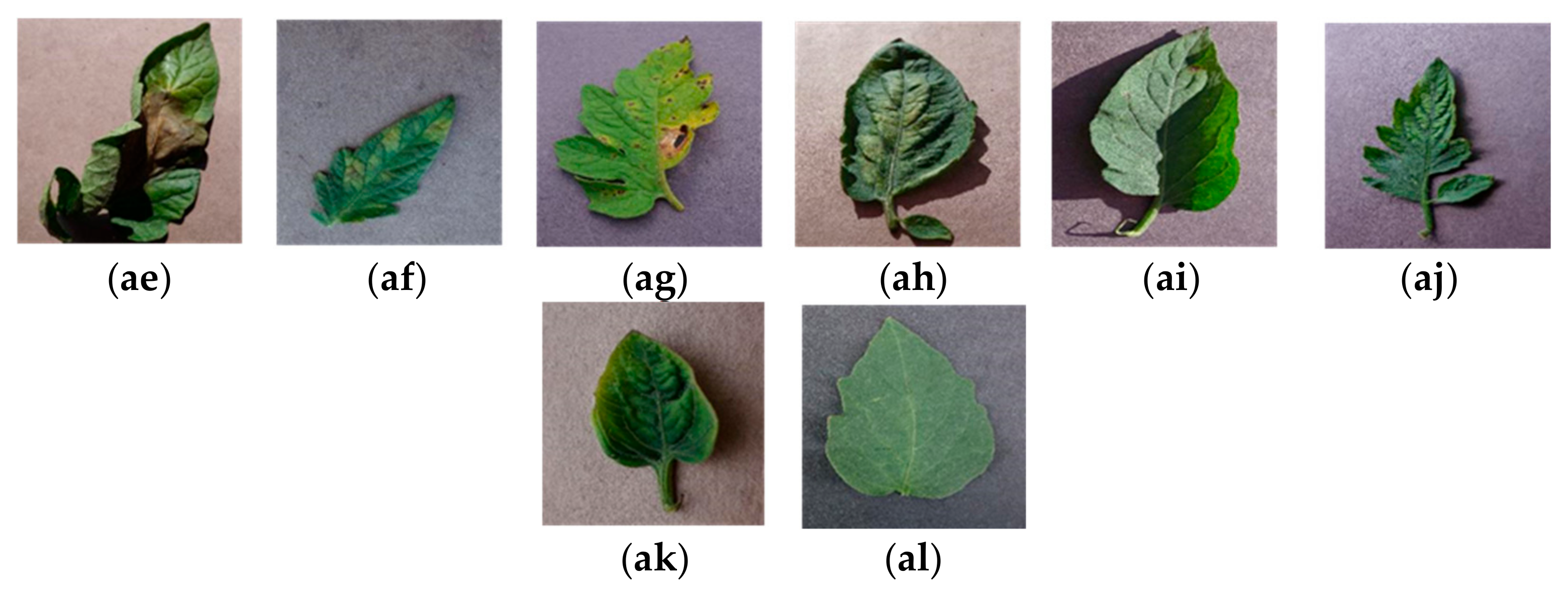
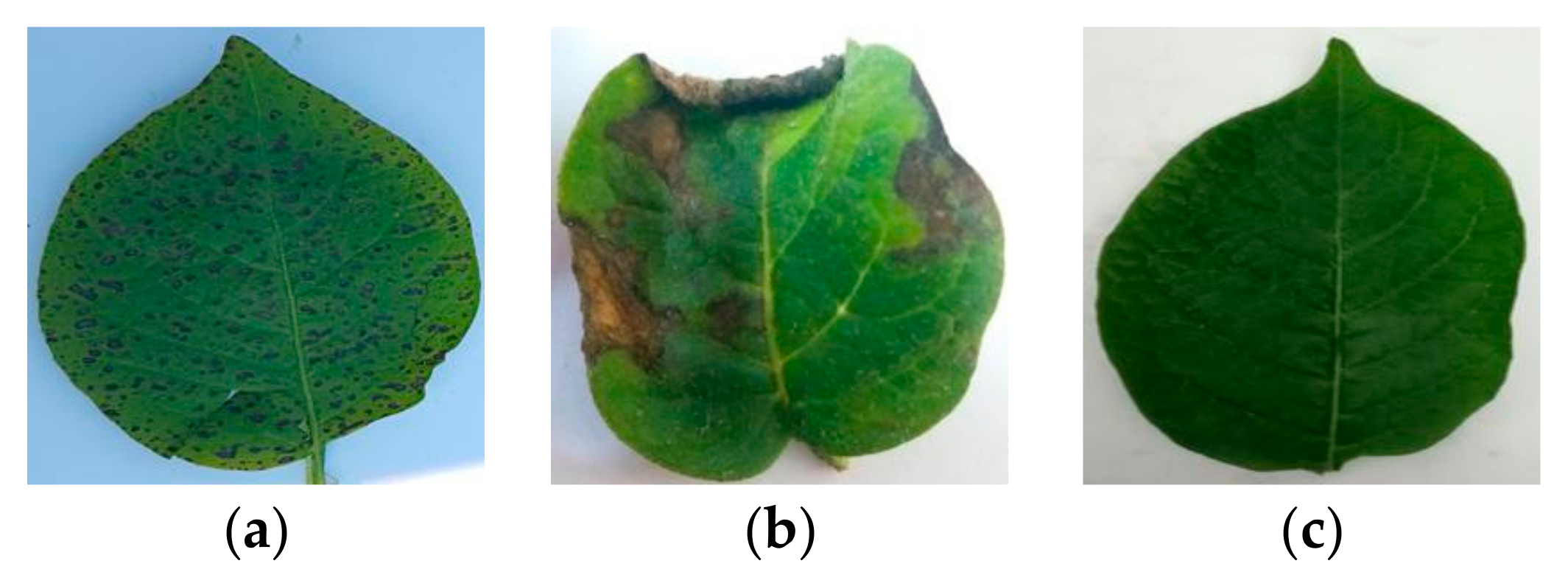
The samples of each class from the PlantVillage and Potato Leaf Disease datasets are given in Figure 1 and Figure 2, respectively.
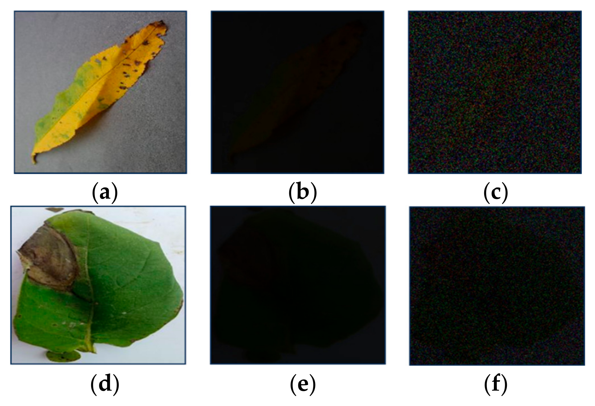
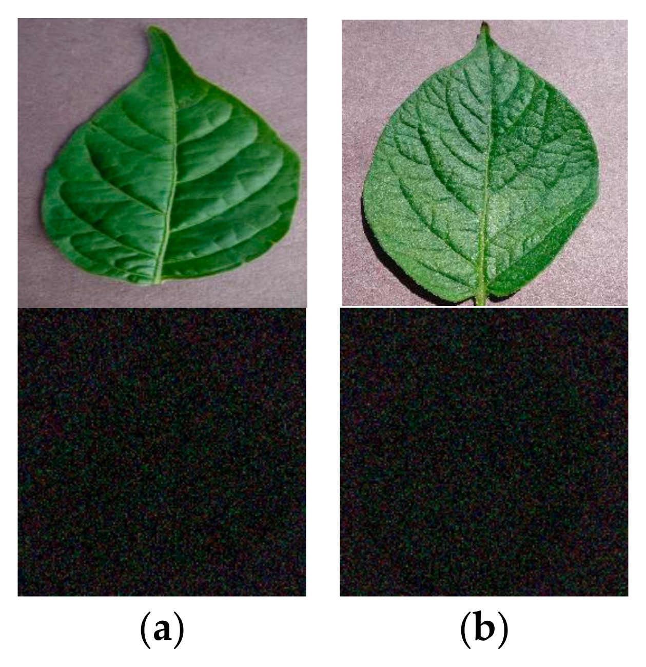
No open database exists for the classification of plant diseases in low-illumination environments, and collecting an actual database in such an environment without agricultural experts on plant diseases is very difficult. Therefore, we synthesized low-light datasets from two open databases using Equation (1). This process contains three basic operations: First, the RGB image is converted into the HSV color space, and then gamma correction is applied to the V-channel. This gamma-corrected image is passed as an input to the Gaussian blur function and then converted back into RGB with the addition of Gaussian noise to create a low-light noisy image [29].
I l o w l i g h t   n o i s y = G B   S ·   I v γ +   G N ( μ , σ 2 )
where G B is a Gaussian blur function, I v is the V-channel value of the HSV image, G N is a Gaussian noise function based on the mean μ and standard deviation σ , and S and γ are gamma correction parameters. The input and final synthesized images of peach bacterial spots from the PlantVillage dataset and potato late blight class from the Potato Leaf Disease dataset are shown in Figure 3.

2.2. Overview of the Proposed Method

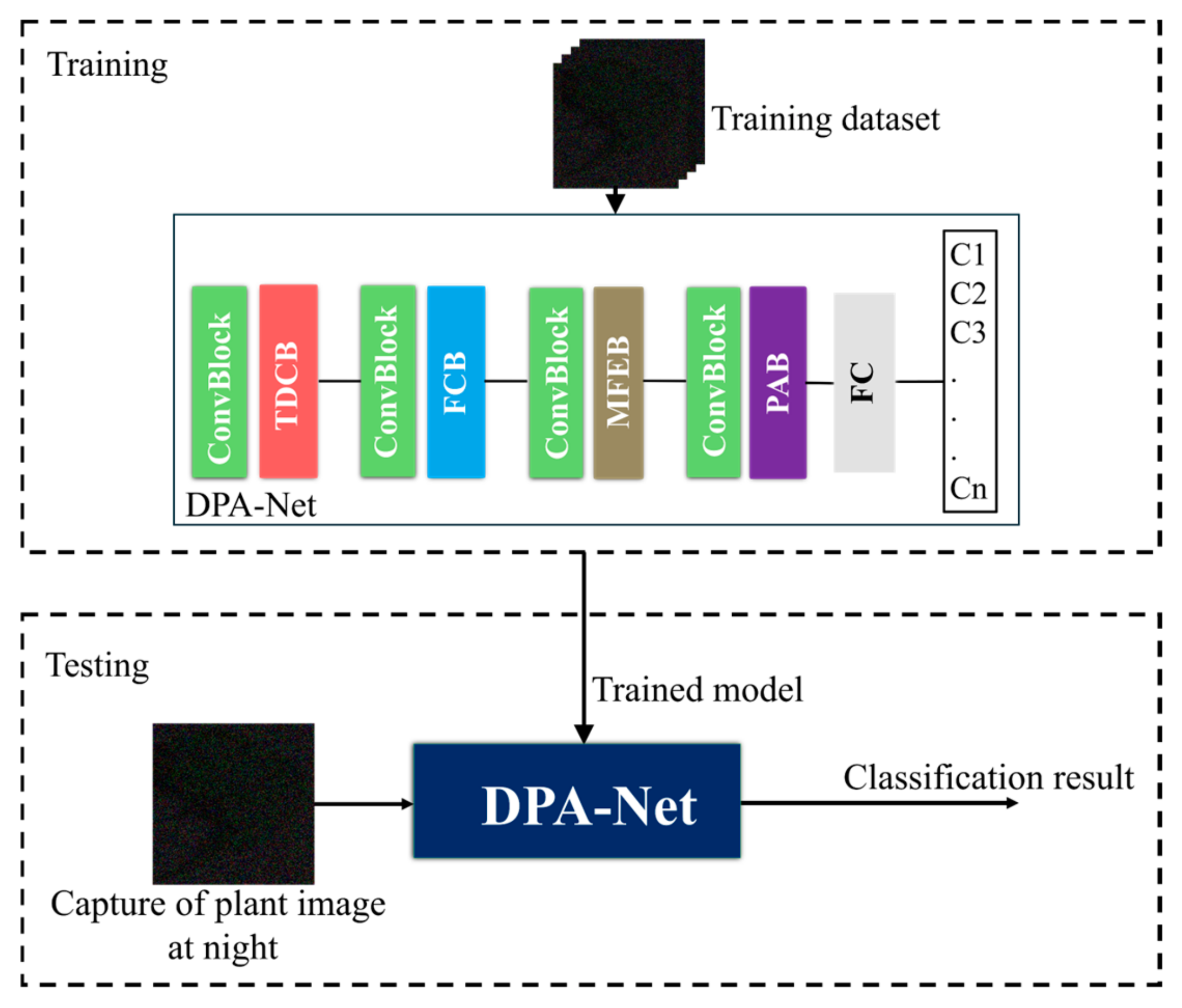
Figure 4 shows an overview of the proposed method for plant disease classification under low-light, noisy environments. First, we perform the training and validation of DPA-Net on low-light noisy images and then classify the test images using the output of DPA-Net.

2.3. DPA-Net Structure

The proposed model, DPA-Net, comprises three new blocks: (1) TDCB, (2) FCB, and (3) MFEB and pixel attention block (PAB), as shown in Figure 5. The structural representation of each block is as follows.
Initially, an input image (I) of size 224 × 224 × 3 pixels is processed with a convolution layer to produce 96 output filters and reduce the spatial dimension using a stride of 4. This layer produces the output tensor F   R 56   ×   56   ×   96 , which is passed to the first stage of the network that includes ConvN Block, a building block of ConvNext [30], repeated three times, and followed by the TDCB. This novel block, TDCB, is responsible for extracting low-level features using dilated convolutions with a wider receptive area and focuses on important regions. The output tensor size of this block is F T D ( o )     R 56   ×   56   ×   96 . The resultant of the TDCB is further processed by the second stage of the network in which down sampling is performed with a convolution layer having a stride of 2 and 192 output filters to produce the tensor F   R 28   ×   28   ×   192 . This is followed by ConvN Block, which is also repeated three times. After this stage, we place another proposed block, FCB, which fuses two convolution layers: the first layer extracts the features, and the second layer applies attention to the extracted features. This is useful for our proposed method, DPA-Net, to learn various patterns. The third and fourth stages of the network also contain down sampling and the ConvN Block, which are repeated 27 and 3 times, respectively. In the third stage, down sampling reduces the spatial dimension of tensor as F   R 14   ×   14   ×   384 , and in the fourth stage, it becomes F   R 14   ×   14   ×   768 . After the third stage, we add an MFEB to extract deep-level features using multipath convolution layers with pixel-level information. This block enables the model to learn complex patterns. The fourth block is placed after the last stage of the network and consists of a simple pixel attention mechanism using a 1 × 1 convolution followed by a sigmoid activation function. Subsequently, the attention generated by the sigmoid function is applied to the input feature using element-wise multiplication. The spatial dimensions of the MFEB and PAB are similar to those of the third and fourth stages, respectively. A head block is placed at the end of the network, consisting of a global average pooling (GAP) and a linear layer used for the purpose classification. We provide a more detailed explanation of each block in the following subsections.

2.3.1. TDCB

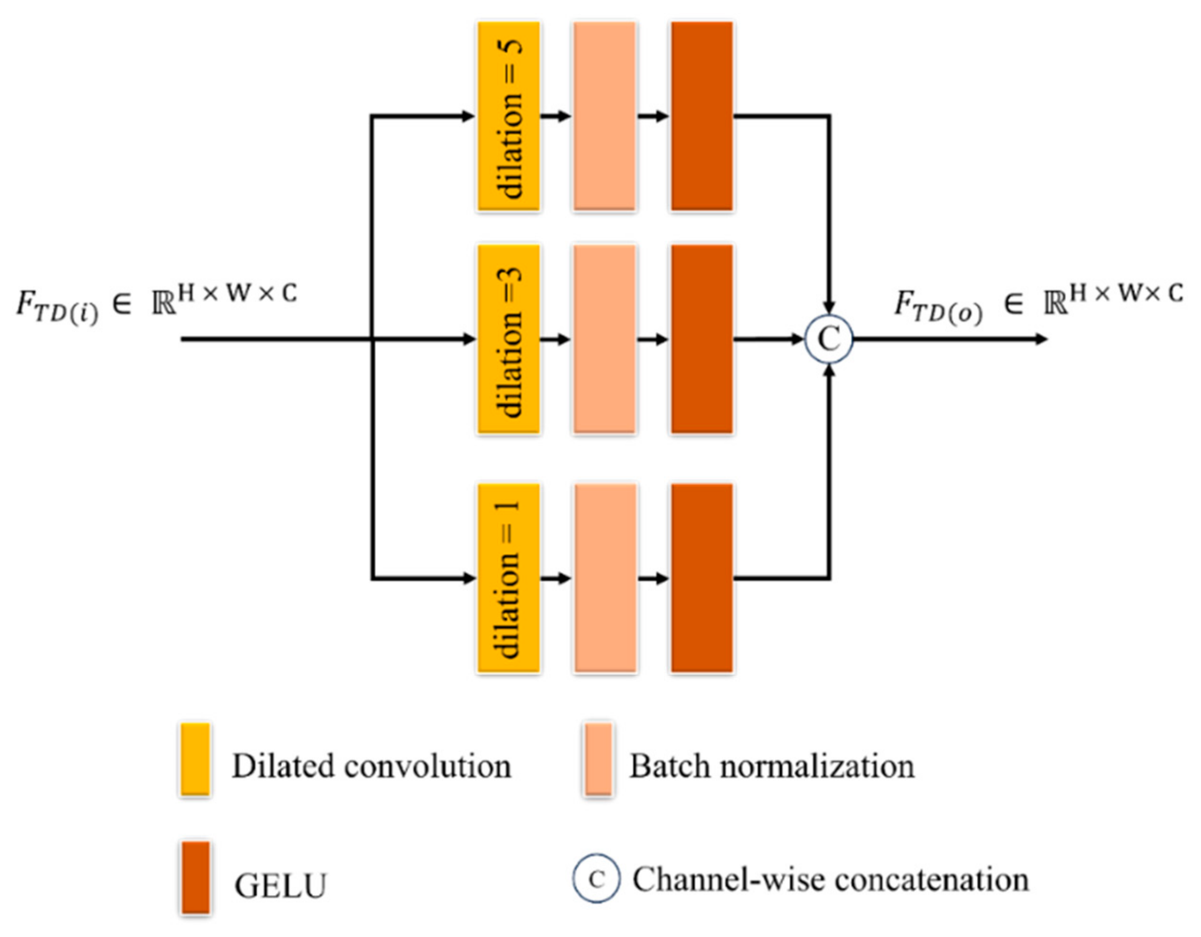
We place the TDCB after the first stage of DPA-Net to extract low-level features with local and global contextual information. The TDCB aids the model in concentrating on disease patterns while considering the edge information of leaves. Using a wider receptive area and signal consistency, it differentiates relevant features from noisy images with low illumination. Additionally, TDCB maintains details and enhances noise robustness while maintaining low parameters in low-light and noisy environments. This block consists of three dilated convolution layers with a kernel size of k = 3 and dilation rates of 1, 3, and 5. A batch normalization (BN) layer comes after each dilated convolution layer, followed by an activation function, the Gaussian error linear unit (GELU), as shown in Figure 6. A dilated convolution is used to capture global and local contextual information from the input without increasing the parameters. If the input feature vector to the F T D ( i )     R H   ×   W   ×   C , then the output feature vector F T D ( o )     R H   ×   W   ×   C can be calculated mathematically using Equation (2), which shows the concatenation operation among three dilated layers after passing through the BN and GELU, respectively. The dilated convolution is expressed in Equation (3).
F T D o = [ D i l C o n v n = 1 ( F T D i   f b a   ( h , w ) )   ©   D i l C o n v n = 3 ( F T D i   f b a   ( h , w ) )         ©   D i l C o n v n = 5 ( F T D i   f b a   ( h , w ) ) ]  
                            D i l C o n v i F i ,   f b a   h , w = h F i b + n   h   f b ( h ) + w F i a + n   w   f a ( w )
where F T D ( o ) is the output feature vector from the TDCB, F T D ( i ) is the input feature vector to the TDCB, f b a   represents convolutional filters, a and b indicate the row and column indexes, respectively, in the spatial dimension of feature F i , h   a n d   w indicate the height and width of the filter, respectively, n is the dilation rate, and © denotes channel-wise concatenation.

2.3.2. FCB

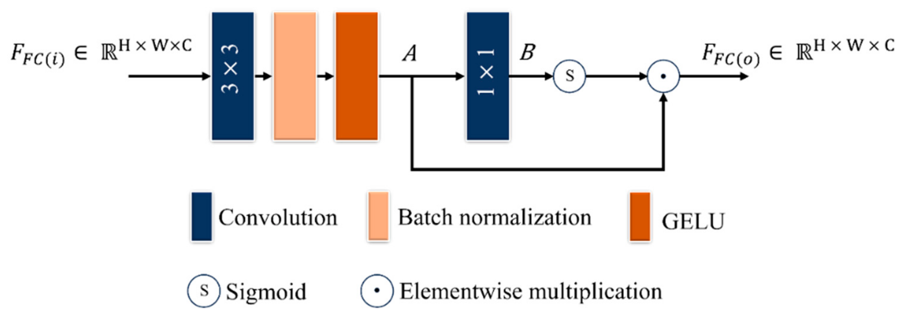
The FCB is added after the second stage of the network to enhance the low contrast by emphasizing the pixel intensities. This block provides information on small and localized areas of leaves where the disease is manifested by focusing on more relevant features. It consists of two convolution layers: the first convolution layer with a kernel size of 3, followed by a BN and GELU. In the second layer, we use a kernel size of 1, followed by a sigmoid, as shown in Figure 7.
Information from both layers is fused by performing element-wise multiplication. This interaction increases the capability of the network to capture complex relationships by considering the nonlinearity and stability with pixel-level information. The extracted output feature vector F F C ( o )     R H   ×   W   ×   C from the FCB can be calculated using Equation (4).
F F C ( o ) R H × W × C = s i g m o i d B A
A R H × W × C   = G E L U ( B N   ( C o n v ( k 3 × 3 ,   F F C ( i ) ) ) )
B     R H × W × C = C o n v k 1 × 1 ,   A
where denotes the elementwise multiplication, and k n × n is the convolution kernel with a size of n × n .

2.3.3. MFEB

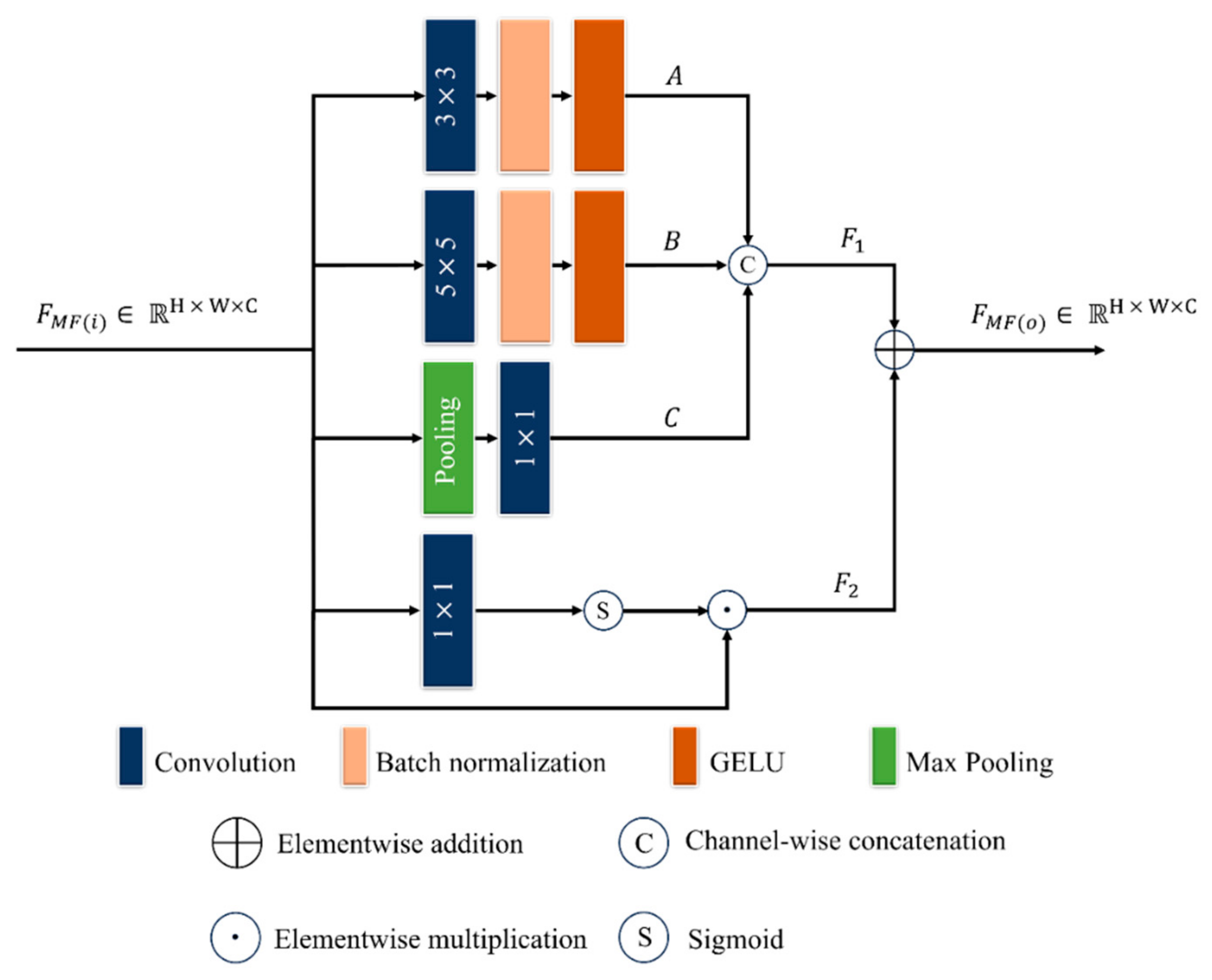
This block is connected after the third stage of the network to extract deep features from the input at the multi-scale level, as shown in Figure 8. It comprises four parallel layers that capture features at different spatial scales. The first and second convolution layers effectively capture the local and global patterns and details. Both layers are followed by a BN and GELU with kernel sizes of 3 × 3 and 5 × 5, respectively, to provide different spatial scales. In the third layer, max pooling is used to reduce the size of the spatial dimensions while preserving its ability to recognize patterns without considering the position. In the fourth convolutional layer, a 1 × 1 kernel was used, followed by a sigmoid activation function. Element-wise multiplication is performed between the input feature and the output of the sigmoid to obtain pixel-level information for the context-aware representation of features. Pixel-level details are added to the concatenated results of the first three layers to obtain multi-scale information and integrate them into a single feature representation.
If the input feature vector to the MFEB is F M F ( i )     R H   ×   W   ×   C , the output feature vector F M F ( o )     R H   ×   W   ×   C can be expressed using Equation (7).
F M F ( o )     R H × W × C = F 1 F 2
F 1     R H × W × C = A   ©   B   ©   C
A   R H × W × C = G E L U B N C o n v k 3 × 3 ,   F M F i
B   R H × W × C = G E L U ( B N   ( C o n v ( k 5 × 5 ,   F M F ( i ) ) ) )
C   R H × W × C = C o n v ( k 1 × 1 ,   M a x P o o l i n g ( F M F ( i ) ) ) )
F 2     R H × W × C   = S i g m o i d C o n v k 1 × 1 ,   F M F i F M F i
where denotes elementwise multiplication, © is channel-wise concatenation, is elementwise addition, and k n × n is a convolution kernel of size n × n .

2.3.4. PAB

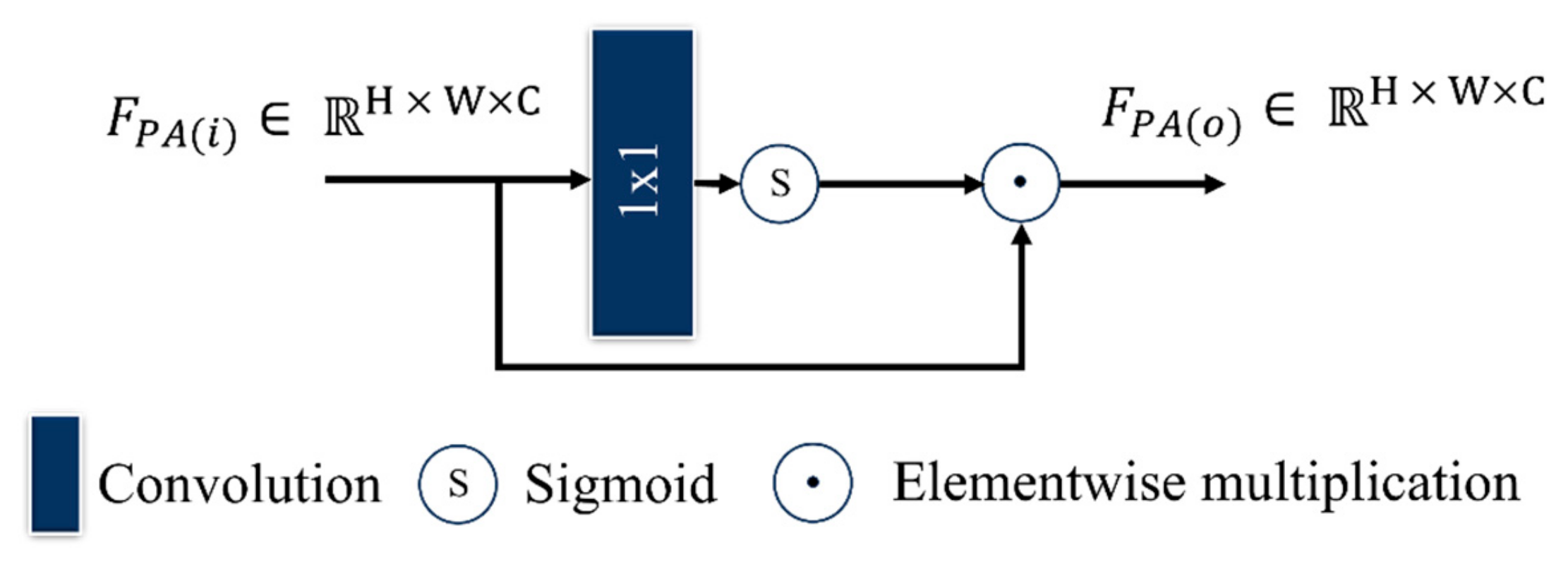
The PAB is introduced after the fourth stage of the network to extract high-level features by incorporating a pixel-level attention mechanism, as shown in Figure 9. The input feature is convolved using a simple convolution layer with a kernel size of 1 × 1, which is then passed through a sigmoid activation function. The convolution layer maps a pixel of the input feature to that of the output feature. The subsequent sigmoid function assigns an attention coefficient to each pixel, indicating its importance in the feature map. This attention map is applied to the input feature F P A ( i ) via element-wise multiplication, and each pixel of the input is modulated by the attention coefficient generated by the sigmoid function. The mathematical notation is expressed using Equation (13).
    F P A ( o ) R H × W × C = S i g m o i d C o n v k 1 × 1 ,   F P A i F P A i
where denotes the elementwise multiplication, and k 1 × 1 is a convolution kernel of size 1 × 1 .

3. Experimental Results

3.1. Training Details

We adopted a data-splitting approach before training the proposed network. Both datasets were divided into 72% training, 8% validation, and 20% testing, and five-fold cross-validation was used to generalize the model to unseen data. To train the hyperparameters, we set a learning rate of 0.0001, the number of epochs to 100, and a batch size of 8. We adopted an adaptive moment estimation (Adam) optimizer [31] and cross-entropy loss [32]. An early stopping method was employed to avoid excessive training of the model, which aided in solving the problem of overfitting and reduced the training time. In this method, a value such as the validation accuracy is considered as the stopping criterion. We plotted the curves for the accuracy and loss of training and validation using our proposed model, as given in Figure 10. Our model not only avoided overfitting problems in the training data, as shown by the convergence of the validation curves, but also successfully trained with the training data, as shown by the convergence of the training curves. The training was stopped when the validation accuracy did not increase over 10 successive epochs. The validation loss for the first dataset in Figure 10 began at a high value, but over the duration of the next few epochs, it significantly decreased and stabilized. The training accuracy increased consistently and reached its peak value when the training loss decreased.

3.2. Evaluation Metrics

The proposed model was evaluated using four parameters: Accuracy, Precision, Recall, and F1-score [4]. These parameters were computed using the values of true positive (TP), true negative (TN), false positive (FP), and false negative (FN) values. TP and TN indicated correct predictions for the positive and negative samples, respectively. FP was a positive prediction made by the model with the actual label being negative. Similarly, FN was a negative prediction made by the model for a positive label. Here, a positive sample refers to an image belonging to the correct class, whereas a negative sample denotes an image belonging to other classes. The sum of TP and TN was the correct prediction made by the model, and the sum of the incorrectly classified instances was the sum of FP and FN. The accuracy was measured as the ratio of correct predictions to the total number of predictions. The F1-score can be calculated as the harmonic mean of the precision and recall, which provides a more inclusive evaluation. The mathematical expressions for the evaluation parameters are given in Equations (14)–(17):
A c c u r a c y   = 1 n i = 1 n   T P i + T N i T P i + T N i + F P i + F N i
P r e c i s i o n   = 1 n i = 1 n   T P i T P i + F P i
R e c a l l   = 1 n i = 1 n   T P i T P i + F N i
F 1 - s c o r e   =   2 × P r e c i s i o n × R e c a l l   P r e c i s i o n + R e c a l l
where n denotes the total number of classes in the dataset.

3.3. Fractal Dimension Estimation

Fractal dimension (FD) is a mathematical metric used to quantitatively analyze complex geometric shapes. Concurrently, multiple studies on fractals have already attracted the attention of researchers for DL-based computer vision tasks [33,34,35,36]. Despite the fact that numerous studies use similar FD estimation methods, their application and interpretation vary greatly across fields, including agriculture, materials science, medical imaging, bioinformatics [37,38,39,40]. One of the applications of FD estimation in the agricultural field is that it provides a way to capture the structural complexity and irregularities of plant leaves, making it useful for detecting subtle disease symptoms [41]. In this study, FD estimation is employed on diseased and healthy leaf images to highlight their morphological differences. First, the activated images predicted by our proposed model are converted into binary images, and then FD is calculated using the box-counting method [42]. The mathematical formulation is given in Equation (18).
F D = l i m S   0 l o g ( N ( S ) ) l o g ( 1 / S )      
where N ( S ) shows the number of boxes, S is the scaling factor of the box and F D is the fractal dimension. The value of F D lies between 1 and 2 for all values of S > 0 , and a higher value shows greater complexity of the shape. The detailed steps involved in F D estimation are given in Algorithm 1.
Algorithm 1: Procedure for estimating FD
Input: I: Binary activated image derived from the proposed DPA-Net
Output: F D : Fractal dimension
Step 1:Set the size of box to the largest dimensions aligned with the nearest power of 2.
   S = 2 ^[log(max(size(I)))/log2]
Step 2:Make the dimensions of I equal to the S using padding
  if size(I) < size( S ):
   padding (I) = S
  end
Step 3:Assign the starting number of boxes
  k = zeros(1, S +1)
Step 4:Count the number of boxes K( S ) containing at least one pixel of diseased area
  k( S +1) = sum(I(:))
Step 5:while S > 1:
  I. Reduce the size of box as S = S /2
  II. Compute again K( S )
end
Step 6:Calculate log( N ( S ) ) and log(1/ S ) for each value of S
Step 7:Determine the best-fit line for [log( N ( S ) ), log(1/ S )] using least square regression.
Step 8:The slop of fitted line is fractal dimension F D
  Return F D

3.4. Ablation Study

In the ablation study, we measured the efficiency of the proposed model with different combinations of the proposed blocks using evaluation metrics. Seven different cases were considered in the ablation study, as listed in Table 4. In Case 1, we trained our model using the same hyperparameters without any proposed blocks to obtain the base performance. In Cases 2–5, we trained our proposed model with only the DCB, FCB, MFEB, and PAB, respectively, to observe the performance of the individual blocks. For Case 2, we considered dilation rates of 1, 3, and 5 for the different receptive areas. As shown in Table 4, each block affected the overall performance of the model. For example, Case 2 had a 0.95% increment in accuracy from the base model, and Case 3 had a 1.05% higher accuracy than the base model. In Case 6, the combination of two blocks, DCB and FCB, was considered because DCB and FCB have a greater effect on performance enhancement than the other blocks, as observed in Cases 2–5, which also exhibited a significant change in performance with respect to the base model. This case provided information about the disease pattern along the edges of the leaf and small regions of the affected area, while considering low-frequency information. In Case 7, the MFEB was added along with the other two blocks, the DCB and FCB. This case had a slightly higher accuracy than Case 6 owing to the multi-scale feature extraction by the MFEB. Finally, we placed all our proposed blocks together and measured the final accuracy, which was the highest among all the cases presented in the ablation study (Table 4).
Another ablation study performed using TDCB at different dilation rates is presented in Table 5. Dilate rate sequences 1, 4, and 6 increased the receptive field rapidly, which enabled the model to capture more spatial information; however, the gap between dilation rates 1 and 4 was large, owing to which mid-level features could possibly be missed, and the overall accuracy decreased compared with the cases of dilate rate sequences 1, 3, and 5. Although the dilation rates of 1, 2, and 4 increased the receptive field, they were not effective in capturing spatial information precisely and exhibited low accuracy. In the proposed model, we used dilation rates of 1, 3, and 5, which is a more balanced approach, enabling the network to capture the fine details and broader context effectively and exhibit the highest performance, as shown in the last row of Table 5.
We also evaluated the performance of the proposed DPA-Net by varying the number of dilation layers in the TDCB, as listed in Table 6. Remarkably, the results of our study showed that the optimal performance of our model was obtained with three dilation layers at rates of 1, 3, and 5. The performance of the model decreased when the number of dilation layers were either decreased or increased. For the two layers, we set the dilation rates to 3 and 5, whereas for the four layers, the rates were 1, 3, 5, and 7.
Furthermore, an ablation study of the FCB was performed to evaluate our proposed model, and the results are presented in Table 7. The FCB consists of the fusion of two convolution layers of 3 × 3 and 1 × 1, respectively, as shown in Figure 7. We considered three methods in this study. Individually, both layers exhibited good performance and high accuracy compared with the base model of Case 1, shown in Table 4, but not higher than the proposed model. As shown in the third row of Table 7, the attention generated by the second convolution layer of 1 × 1 was not applied to the feature map produced by the first convolutional layer of 3 × 3 because its performance was slightly lower than that of the proposed model. Although the performance improved slightly with attention, the main advantage was that the trainable parameters remained unchanged.
Additionally, an ablation study on the MFEB was performed to validate the effectiveness of our proposed model, and the results are presented in Table 8. The MFEB consists of four parallel layers for extracting features at different scales, as shown in Figure 8. We used four different methods in this ablation study to evaluate the effect on the performance without each layer. The results showed that without A and B in Figure 5, the accuracy decreased from that of the proposed model, indicating that these parallel layers extracted crucial features that contributed to the overall performance. Without the third parallel layer (C in Figure 8), the accuracy was very close to that of the proposed layer, implying that its contribution was less significant. In the last method without F2 in Figure 8, which was simple pixel attention, the accuracy also decreased compared with the proposed model, indicating that pixel-level information also contributes significantly to the overall performance of the proposed method.
Table 9 compares the performance of the proposed method on the Potato Leaf Disease Dataset across different learning rates and batch sizes. It is clearly shown from rows 1 to 4 that increasing or decreasing the learning rate and batch size from the proposed values resulted in lower performance. Therefore, a learning rate of 0.0001 and a batch size of 8 were selected as the optimal hyperparameters for the proposed method.

3.5. Comparison of DPA-Net with State-of-the-Art (SOTA) Methods

We evaluated the effectiveness of our proposed model by comparing it with different SOTA methods. For fair comparison, we considered the same experimental protocols by using low-light images and five-fold cross-validation for both datasets. Table 10 shows that the proposed DPA-Net consistently outperformed the SOTA methods on the PlantVillage dataset. The outstanding performance of the DPA-Net can be recognized for its capability to distinguish related features from low-illumination noisy images. In addition, the FCB of DPA-Net enhances the contrast and focuses on the disease-affected region to create an effective classification model for plant disease in a low-illumination environment.
Details of the performance comparisons of the proposed model with the SOTA methods on the Potato Leaf Disease dataset are listed in Table 11. Our proposed model performed exceptionally well for potato disease classification. Our method had higher accuracy by 6.32% and higher F1-score by 6.37% than the second-best method (ConvNext-small). The reasons for the low performance by shifted window transformer (Swin-T) [54] is as follows: Swin-T requires large-scale data for effective generalization. As the Potato Leaf Disease dataset contains only 4072 images, it exhibited poor performance. The reasons for the poor performance of SqueezeNet and AlexNet are as follows: The performance of AlexNet is unsatisfactory because it is relatively shallow, restricting its capacity for complex feature extraction. SqueezeNet is also a lightweight and computationally effective network but struggles with complex feature extraction in a low-light noisy environment. As shown in Table 11, it did not have optimal performance owing to its limited feature extraction capability.

3.6. Comparisons of Model Complexity

For complexity comparison, we considered four important metrics: the number of trainable parameters (#param), the floating-point operations (FLOPs), memory usage, and processing time per image. Comparisons of the first three metrics for the PlantVillage and Potato Leaf Disease datasets are presented in Table 12 and Table 13, respectively. Although our proposed model, DPA-Net, had a lower performance in terms of model complexity for both datasets, as shown in Table 12 and Table 13, it outperformed the SOTA methods in correctly classifying plant disease with low-light noisy images while exhibiting a high accuracy and F1-score, as shown in Table 10 and Table 11. We tested the same SOTA methods on both datasets, and the computational complexity for the second dataset was slightly lower owing to the difference in the number of classes. As mentioned in Section 2.1, the PlantVillage dataset has 38 classes, and the Potato Leaf Disease dataset contains only 3 classes.
The comparative results of the processing time in the embedded system environment of the Jetson TX2 along with the desktop computer are listed in Table 14. The Jetson TX2 has a 256-core NVIDIA PascalTM GPU architecture, equipped with 256 NVIDIA compute unified device architecture (CUDA) cores. The memory of 8 GB is shared between the GPU and central processing unit (CPU), and it requires a minimum power of 7.5 W to operate [66]. The specifications of the desktop computer are given in Section 2.1. Jetson TX2 embedded systems can be used in agricultural mobile robots or mobile devices with cameras for the real-time monitoring of crop health by utilizing edge computing. As shown in Table 14, our method had a processing speed of 97.5 (1000/10.26) frames per second (FPS) and 10.4 (1000/96.29) FPS in the desktop computer and Jetson TX2 embedded system, respectively. Although our method did not exhibit the best performance in terms of processing time, it outperformed the SOTA methods in correctly classifying plant diseases with low-light noisy images while exhibiting a high accuracy and F1-score. Moreover, we confirmed that the proposed method can be operational within an embedded system that has constrained computational capabilities.

4. Discussion

4.1. Confusion Matrices, Robustness to the Illumination and Noise Level, and Experiments with Real Low-Illumination Dataset

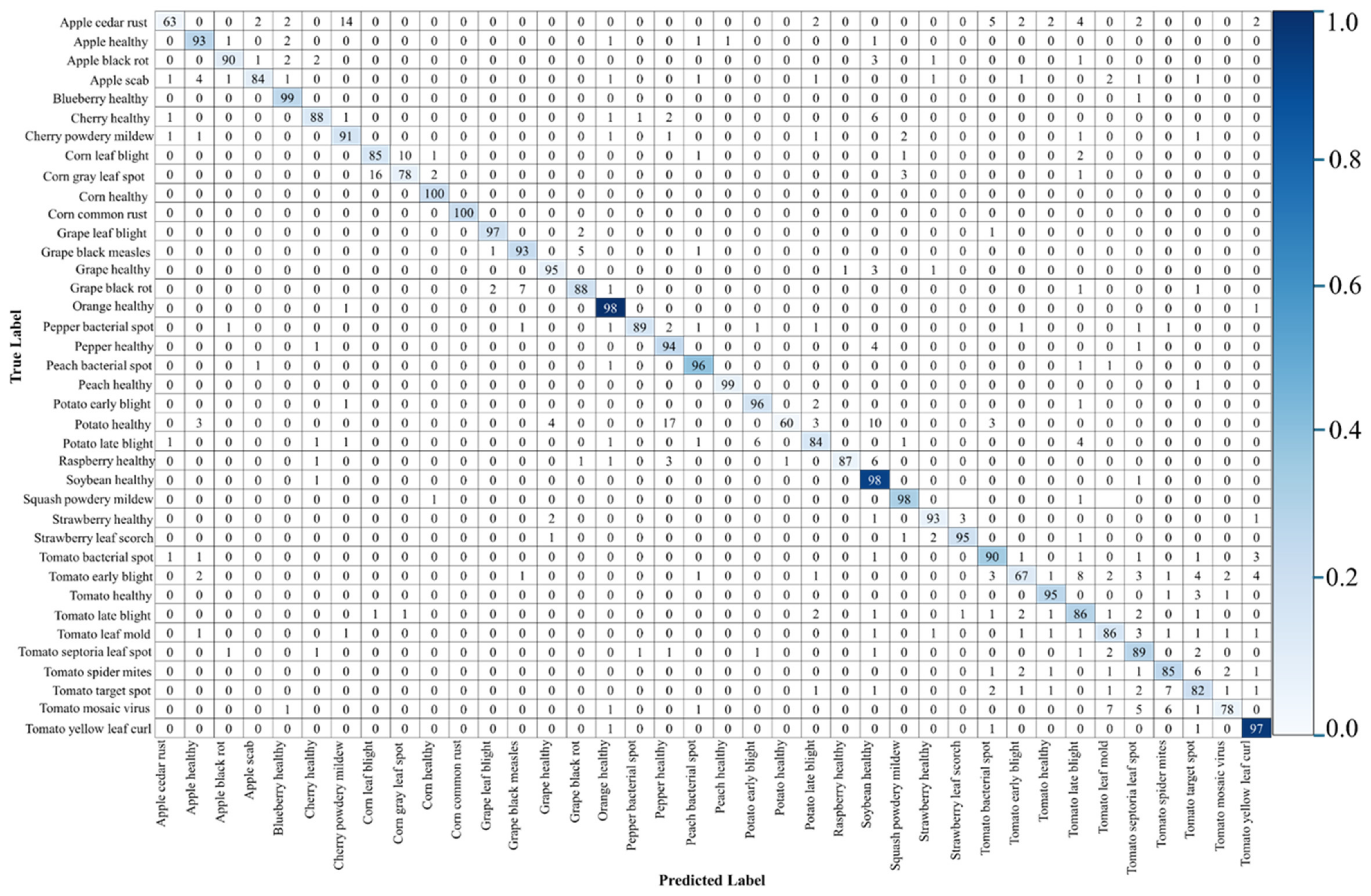
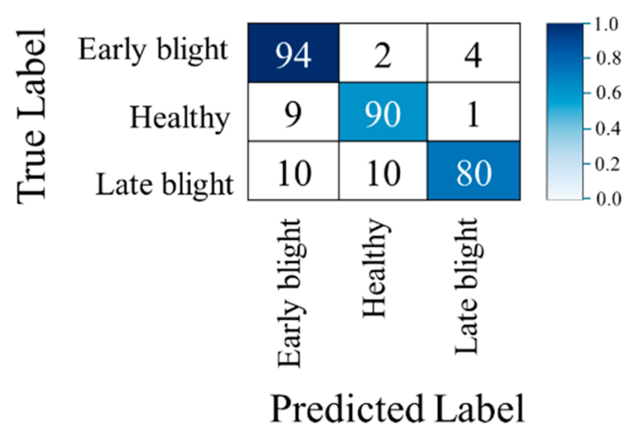
A confusion matrix presents a summary of the predictions made by a model in matrix form [67]. It shows the correct and incorrect predictions with respect to a class. In this matrix, all the diagonal values are TP for the corresponding classes, whereas the horizontal and vertical values without diagonal instances are FP and FN, respectively. All diagonal values without the TP of a particular class are TN. After testing our proposed model, DPA-Net, on the PlantVillage and Potato Leaf Disease datasets, we generated confusion matrices, as shown in Figure 11 and Figure 12, respectively. The figures show that our model effectively predicted the correct labels. We present the robustness of DPA-Net to illumination and noise levels for the Potato Leaf Disease dataset in Table 15. Different values of S, γ, and σ were tested to analyze their impact on performance, and our model maintains stability across varying illumination and noise levels.
For the experiments on the real low-illumination dataset, we selected a total of 300 images, 100 from each class of the Potato Leaf Disease dataset [27]. These images were then printed using SAM-SUNG SL-C3510ND printer [68]. The printed images were subsequently captured using Samsung A23 smart phone [69] at night with no moon. During the image capture, illumination level was 0 lux, as measured using light meter LM-81LX [70]. For the training on this low-illumination dataset, we used the same data split as the other two datasets: 72% for training, 8% for validation, and 20% for testing. Since the Potato Leaf Disease Dataset has three classes with predefined labels, namely early blight, late blight, and healthy, the original labels were retained during image capture. After training and testing DPA-Net on this real low-illumination dataset using two-fold cross-validation as given in Table 16, we obtained results comparable to those on low-light Potato Leaf Disease dataset of Table 11. Although images of both datasets contain plain backgrounds, there are lots of samples that contain severe shadows and poor illumination, reflecting the concept of a low-light and noisy environment for field-collected validation, as shown in Figure 13.

4.2. Statistical Analyses, and Grad-CAM

Additionally, we performed a t-test [71] and calculated Cohen’s d-value [72] to demonstrate the statistical significance of the variance in the classification accuracy between DPA-Net and the second-best model. We obtained p-values of 0.019 and 0.00389 for the PlantVillage and Potato Leaf Disease datasets, respectively, with confidence levels of 95% and 99%, respectively. Typically, a Cohen’s d-value of 0.8 indicates a large effect size, 0.5 signifies a medium effect, and 0.2 represents a small effect. We obtained Cohen’s d-values of 1.85 and 1.57 for the PlantVillage and the Potato Leaf Disease datasets, respectively, demonstrating a large effect size. Based on these results, we verify that our method achieved significantly higher accuracy compared to the SOTA methods.
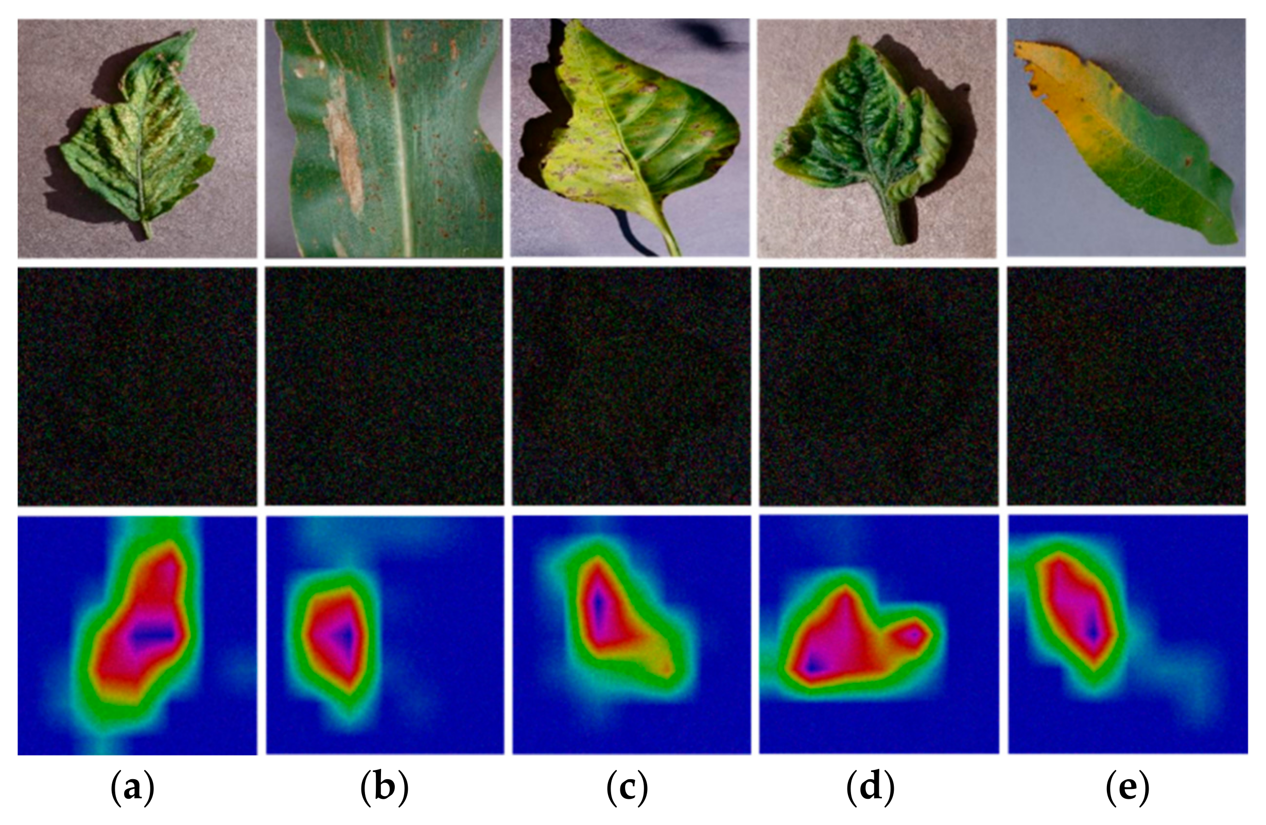
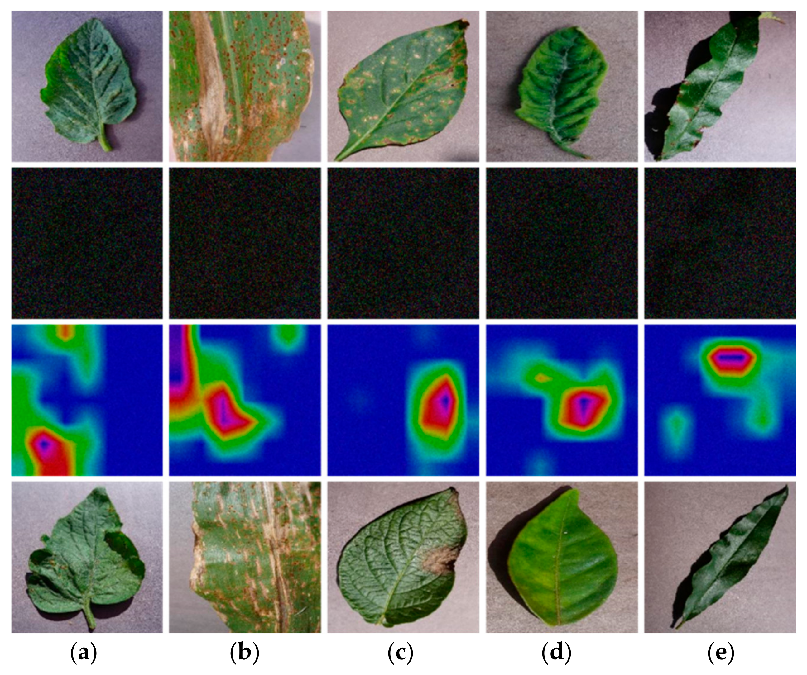
For a more detailed analysis, we utilized the Grad-CAM technique [73], which is a notable tool for visualizing and highlighting the important features in samples that impact the model’s performance. Using this technique, the model focuses on important regions when making predictions. We considered the last-stage PAB of DPA-Net to generate Grad-CAM heat maps and identified the samples to determine whether they were correctly or incorrectly classified. The results of the correctly classified samples are shown in Figure 14 and Figure 15 for the PlantVillage and Potato Leaf Disease datasets, respectively. This reveals that the model pays attention to the disease-affected regions in different plant leaves. Each row from top to bottom shows the original image, low-light noisy image, and corresponding Grad-CAM generated using DPA-Net. The red region in the heatmap indicates the high confidence of the model in categorizing the samples as disease-affected leaves. In contrast, the color change from green to blue in the heat map indicates less confidence in the prediction of the disease area and increased uncertainty in identifying the correct disease label. For a healthy class, the entire leaf exhibits the same green color and no symptoms of disease, which is why the proposed model focuses on a complete leaf and correctly classifies it, as shown in Figure 15c.

4.3. Performance Evaluation of DPA-Net by FD Estimation

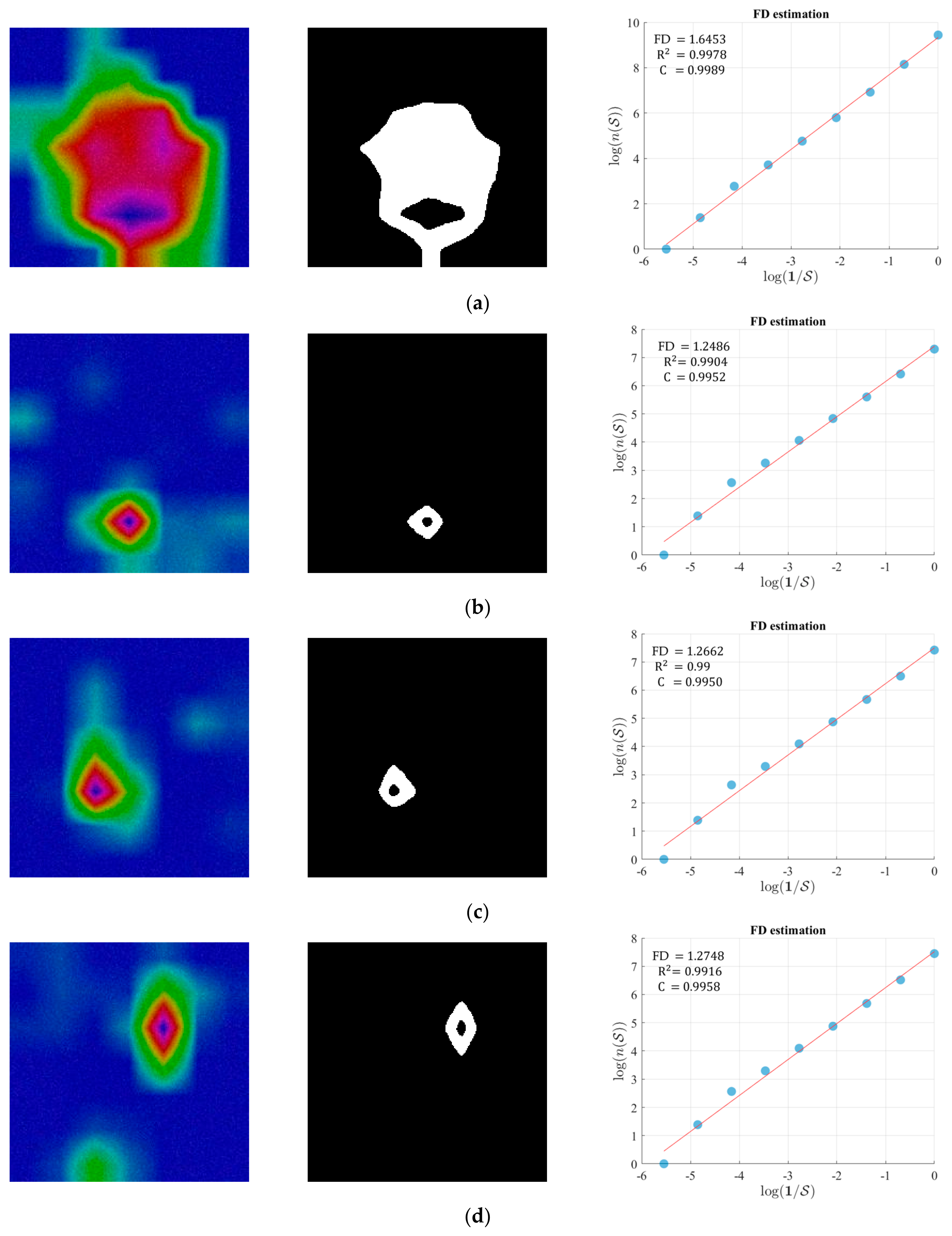
For further performance assessment, we performed FD estimation to analyze the regions focused on by our proposed model. This approach captures the structural complexity and irregularities of the given region numerically, thereby reinforcing the decision of our classification model. From Algorithm 1 of Section 3.3, we adopted the box-counting method, where binarized activated images are used as input to perform FD estimation for diseased and healthy leaf images. As explained in Section 4.2, Grad-CAM is employed to generate heat maps of our model’s predictions, highlighting the most relevant regions. The detailed analysis of FD estimation for diseased and healthy cases is presented in Figure 16. The first column of Figure 16 denotes the Grad-CAM outputs of infected and healthy leaves as predicted by DPA-Net. The middle column displays the binarized versions of their corresponding Grad-CAMs. In these binarized images, the white area shows the region where DPA-Net pays more attention, while the black area indicates a less significant region. From Algorithm 1, boxes of varying sizes and their total counts are calculated, and corresponding FD values are obtained for diseased and healthy leaves as shown in the rightmost column of Figure 16. In addition, we also calculate the coefficient of determination ( R 2 ), and the correlation coefficient (C). R 2 measures how well the data points fit the regression line, with values closer to 1 indicating a better fit. The value of C indicates the correlation between two log values, where values closer to 1 confirm that the FD estimation is valid, as the data strongly follows a straight line. A higher value of FD corresponds to a more complex and irregular structure in a given image. The comparative analysis of FD values, R 2 , and C is summarized in Table 17. The healthy leaf exhibited a higher FD value than all the diseased cases, which reflects greater structural complexity of its original venation. In contrast, diseased leaves showed consistently lower FD values, suggesting that morphological details are lost due to disease infection. This comparison of FD values confirms that our proposed model is effectively classifying healthy and diseased leaves using low-light noisy images.

4.4. Integration of FD in Classification Results

We integrate FD analysis into the classification results of our proposed DPA-Net to evaluate its performance. For this purpose, we consider a threshold value of 1.60 for FD to determine whether the input image belongs to the healthy or diseased class. The optimal threshold was experimentally determined with training data, with which the highest accuracy was obtained with training data. As discussed earlier in Section 4.3, a higher value of FD indicates a healthy leaf, while a lower value corresponds to a diseased leaf. Based on this, if the FD value of a given input is below the threshold, it is classified as diseased; otherwise, it is considered healthy case. The performance of our proposed model with FD integration on the Potato Leaf Disease Dataset is presented in Table 18. The results clearly indicate enhanced performance, with accuracy improving by 4.76% and F1-score increasing by 7.26%. FD integration confirms that our method effectively differentiates between healthy and diseased leaves under low-light, noisy conditions.

5. Limitations of the Proposed DPA-Net

Despite the remarkable overall performance of the proposed method, the healthy potato class had a significant classification error, with 17% of the samples misclassified as healthy peppers (Figure 11). The primary reason for this misclassification was the similarity in features such as leaf shape, color, and texture between the two classes, as shown in Figure 17. Additionally, data imbalance played a role, as the sample size for the healthy pepper class was almost ten times larger than that in the healthy potato class. Another major classification error was observed in apple cedar rust, in which 14% of the samples were misclassified as cherry powdery mildew (Figure 11). Furthermore, the sample size for cherry powdery mildew was almost four times larger than that for apple cedar rust. Owing to these factors, the model cannot easily distinguish between them. DPA-Net had a classification error of 8% for tomato early blight, misclassifying it as tomato late blight (Figure 11). As the disease progresses, symptoms overlap in terms of lesion shape, discoloration of the surrounding areas, and lesion size, making it difficult to differentiate between them.
For the second dataset, our proposed model, DPA-Net, also exhibited some classification errors for late blight potatoes and 10% classification errors for healthy potatoes and early blight potatoes (Figure 12). These three classes, healthy, early blight, and late blight potatoes, exhibited similar leaf texture, color, and early disease symptoms, as shown in Figure 18. Owing to these similar features, it was a challenging task for the DPA-Net to correctly classify them. Figure 19 and Figure 20 show the critical assessment of disease samples from a specific class that were misclassified as other classes by DPA-Net for the PlantVillage and Potato Leaf Disease datasets, respectively.
Figure 19a shows a sample of the tomato spider mite class, but it was misclassified as a tomato target spot because the leaf texture and color are similar because both belong to the same plant. Disease-affected pixels are similar and present at different locations on leaves in both classes, owing to which model attention was dispersed, resulting in misclassification. Figure 19b shows a sample of corn northern leaf blight; however, DPA-Net predicted it to be corn common rust. Disease spots in both classes are common and appear similar in terms of pixel color and pattern. Both leaves have similar disease spots and connected regions at various locations, which was the reason for incorrect classification. Figure 19c shows an image of a pepper bacterial spot that was incorrectly classified as potato late blight. Pepper leaves have several small dark spots with a yellowish tinge around some spots, whereas potato leaves have dark water-soaked lesions. If the bacterial spots coalesce, they resemble larger blight lesions. The color and texture of lesions become considerably similar under the same lighting conditions, making it challenging for our proposed model to identify them precisely. Figure 19d shows an example of a tomato yellow leaf curl virus misclassified as healthy orange. The original image was not completely affected by the virus; only the boundary of the leaf exhibited a yellow color. The area other than the boundary was greenish, similar to orange leaves, and both had protruding patterns in most of the areas. Under these circumstances, DPA-Net yielded misclassification results. Figure 19e shows a sample of a peach leaf that was affected by a bacterial attack, but it was not correctly predicted by DPA-Net and was considered a healthy peach leaf. The green shade, texture, and pattern of the leaves of both samples were closely related. The spots of disease were not as prominent in the original class when compared with the misclassified class that had no spots, and these were obstacles to the accurate categorization of DPA-Net. An illustration of how early potato blight was misclassified as late blight is shown in Figure 20. Late blight disease also causes lesions on leaves, but the size and pattern of the lesions can differ from those of early blight. Potato early blight disease often manifests as small dark water-soaked patches that eventually turn into lesions. Because of the low-light conditions, our proposed model interpreted the two large spots on the right side of the early blight leaf in the provided image as a large late blight lesion, resulting in an incorrect classification.

6. Conclusions

In this paper, we propose DPA-Net for plant disease classification in low-light noisy images, which is the first study on this task. Three new convolution blocks—TDCB, FCB, and MFEB—were introduced in the proposed model. By incorporating these three blocks, the proposed DPA-Net is an innovative model for classifying plant diseases in images captured under low-light and noisy conditions. DPA-Net exhibited a high classification accuracy and F1-score when evaluated on two open datasets. In addition, statistical analysis using the t-test and Cohen’s d-value supports that these improvements are significant. Moreover, we confirmed that our method can be effectively deployed on embedded systems with limited processing capabilities, which can be used in agricultural mobile robots or mobile devices. A Grad-CAM analysis also showed that our model can extract important features for the correct classification of diseases. This enables the real-time monitoring of efficient plant disease management. Moreover, to improve the capability of our proposed system and analyze structural complexity, we performed fractal dimension estimation using Grad-CAM images of diseased and healthy leaves. DPA-Net exhibited a few classification errors owing to similarities in leaf color, textures, and patterns of disease across various classes. For example, northern corn leaf blight was misclassified as corn common rust, pepper bacterial spots as potato late blight, and tomato spider mites as tomato target spots. This was primarily due to the similar disease characteristics and different lighting conditions. The proposed DPA-Net has not been extensively evaluated on real agricultural field images under low-light conditions, and its robustness in complex backgrounds with varying illumination remains to be validated.
We will investigate methods to address these classification errors and limitations by utilizing advanced attention mechanisms that focus on the critical areas of the leaves and relevant features. In addition, we will conduct further research on enhancing low-light noisy images to increase the classification accuracy by utilizing losses related to the characteristics of plant diseases.

Author Contributions

Conceptualization, H.A.H.G.; methodology, H.A.H.G.; validation, S.I.J. and W.H.J.; data curation, J.S.K. and R.A.; software, M.I. and M.H.T.; supervision, K.R.P.; writing—original draft preparation, H.A.H.G.; writing—review and editing, K.R.P. All authors have read and agreed to the published version of the manuscript.

Funding

This work was supported in part by the Ministry of Science and ICT (MSIT), Korea, through the Information Technology Research Center (ITRC) Support Program under Grant IITP-2025-RS-2020-II201789, in part by the Artificial Intelligence Convergence Innovation Human Resources Development Supervised by the Institute of Information & Communications Technology Planning & Evaluation (IITP) under Grant IITP-2025-RS-2023-00254592.

Data Availability Statement

The data supporting the findings of this study are available from the GitHub Repository (https://github.com/gondalalihamza/DPA-Net, accessed on 11 September 2025).

Conflicts of Interest

The authors declare no conflicts of interest.

References

  1. Vásconez, J.P.; Vásconez, I.N.; Moya, V.; Calderón-Díaz, M.J.; Valenzuela, M.; Besoain, X.; Seeger, M.; Auat Cheein, F. Deep Learning-Based Classification of Visual Symptoms of Bacterial Wilt Disease Caused by Ralstonia Solanacearum in Tomato Plants. Comput. Electron. Agric. 2024, 227, 109617. [Google Scholar] [CrossRef]
  2. Tilman, D.; Balzer, C.; Hill, J.; Befort, B.L. Global Food Demand and the Sustainable Intensification of Agriculture. Proc. Natl. Acad. Sci. USA 2011, 108, 20260–20264. [Google Scholar] [CrossRef] [PubMed]
  3. Habib, M.T.; Majumder, A.; Jakaria, A.Z.M.; Akter, M.; Uddin, M.S.; Ahmed, F. Machine Vision Based Papaya Disease Recognition. J. King Saud Univ.—Comput. Inf. Sci. 2020, 32, 300–309. [Google Scholar] [CrossRef]
  4. Sajitha, P.; Andrushia, A.D.; Anand, N.; Naser, M.Z. A Review on Machine Learning and Deep Learning Image-Based Plant Disease Classification for Industrial Farming Systems. J. Ind. Inf. Integr. 2024, 38, 100572. [Google Scholar] [CrossRef]
  5. Shirahatti, J.; Patil, R.; Akulwar, P. A Survey Paper on Plant Disease Identification Using Machine Learning Approach. In Proceedings of the 3rd IEEE International Conference on Communication and Electronics Systems, Coimbatore, India, 15–16 October 2018; pp. 1171–1174. [Google Scholar]
  6. Panigrahi, K.P.; Das, H.; Sahoo, A.K.; Moharana, S.C. Maize Leaf Disease Detection and Classification Using Machine Learning Algorithms. In Proceedings of the Springer Progress in Computing, Analytics and Networking, Singapore, 27 March 2020; pp. 659–669. [Google Scholar]
  7. Bhatia, A.; Chug, A.; Singh, A.P. Application of Extreme Learning Machine in Plant Disease Prediction for Highly Imbalanced Dataset. J. Stat. Manag. Syst. 2020, 23, 1059–1068. [Google Scholar] [CrossRef]
  8. Mathew, A.; Antony, A.; Mahadeshwar, Y.; Khan, T.; Kulkarni, A. Plant Disease Detection Using GLCM Feature Extractor and Voting Classification Approach. Mater. Today Proc. 2022, 58, 407–415. [Google Scholar] [CrossRef]
  9. Panchal, P.; Raman, V.C.; Mantri, S. Plant Diseases Detection and Classification Using Machine Learning Models. In Proceedings of the 4th IEE International Conference on Computational Systems and Information Technology for Sustainable Solution, Bengaluru, India, 20–21 December 2019; pp. 1–6. [Google Scholar]
  10. Thakur, P.S.; Khanna, P.; Sheorey, T.; Ojha, A. Trends in Vision-Based Machine Learning Techniques for Plant Disease Identification: A Systematic Review. Expert Syst. Appl. 2022, 208, 118117. [Google Scholar] [CrossRef]
  11. Wani, J.A.; Sharma, S.; Muzamil, M.; Ahmed, S.; Sharma, S.; Singh, S. Machine Learning and Deep Learning Based Computational Techniques in Automatic Agricultural Diseases Detection: Methodologies, Applications, and Challenges. Arch. Comput. Methods Eng. 2022, 29, 641–677. [Google Scholar] [CrossRef]
  12. Yu, M.; Ma, X.; Guan, H. Recognition Method of Soybean Leaf Diseases Using Residual Neural Network Based on Transfer Learning. Ecol. Inform. 2023, 76, 102096. [Google Scholar] [CrossRef]
  13. Reddy, S.R.G.; Varma, G.P.S.; Davuluri, R.L. Resnet-Based Modified Red Deer Optimization with DLCNN Classifier for Plant Disease Identification and Classification. Comput. Electr. Eng. 2023, 105, 108492. [Google Scholar] [CrossRef]
  14. Kaya, Y.; Gürsoy, E. A Novel Multi-Head CNN Design to Identify Plant Diseases Using the Fusion of RGB Images. Ecol. Inform. 2023, 75, 101998. [Google Scholar] [CrossRef]
  15. Malik, A.; Vaidya, G.; Jagota, V.; Eswaran, S.; Sirohi, A.; Batra, I.; Rakhra, M.; Asenso, E. Design and Evaluation of a Hybrid Technique for Detecting Sunflower Leaf Disease Using Deep Learning Approach. J. Food Qual. 2022, 2022, 9211700. [Google Scholar] [CrossRef]
  16. Guo, M.-H.; Xu, T.-X.; Liu, J.-J.; Liu, Z.-N.; Jiang, P.-T.; Mu, T.-J.; Zhang, S.-H.; Martin, R.R.; Cheng, M.-M.; Hu, S.-M. Attention Mechanisms in Computer Vision: A Survey. Comput. Vis. Media 2022, 8, 331–368. [Google Scholar] [CrossRef]
  17. Yang, W.; Yuan, Y.; Zhang, D.; Zheng, L.; Nie, F. An Effective Image Classification Method for Plant Diseases with Improved Channel Attention Mechanism aECAnet Based on Deep Learning. Symmetry 2024, 16, 451. [Google Scholar] [CrossRef]
  18. Dai, G.; Tian, Z.; Fan, J.; Sunil, C.K.; Dewi, C. DFN-PSAN: Multi-Level Deep Information Feature Fusion Extraction Network for Interpretable Plant Disease Classification. Comput. Electron. Agric. 2024, 216, 108481. [Google Scholar] [CrossRef]
  19. Yang, L.; Yu, X.; Zhang, S.; Long, H.; Zhang, H.; Xu, S.; Liao, Y. GoogLeNet Based on Residual Network and Attention Mechanism Identification of Rice Leaf Diseases. Comput. Electron. Agric. 2023, 204, 107543. [Google Scholar] [CrossRef]
  20. Xu, L.; Cao, B.; Zhao, F.; Ning, S.; Xu, P.; Zhang, W.; Hou, X. Wheat Leaf Disease Identification Based on Deep Learning Algorithms. Physiol. Mol. Plant Pathol. 2023, 123, 101940. [Google Scholar] [CrossRef]
  21. Tang, L.; Yi, J.; Li, X. Improved Multi-Scale Inverse Bottleneck Residual Network Based on Triplet Parallel Attention for Apple Leaf Disease Identification. J. Integr. Agric. 2024, 23, 901–922. [Google Scholar] [CrossRef]
  22. Bi, C.; Xu, S.; Hu, N.; Zhang, S.; Zhu, Z.; Yu, H. Identification Method of Corn Leaf Disease Based on Improved Mobilenetv3 Model. Agronomy 2023, 13, 300. [Google Scholar] [CrossRef]
  23. Nagasubramanian, G.; Sakthivel, R.K.; Patan, R.; Sankayya, M.; Daneshmand, M.; Gandomi, A.H. Ensemble Classification and IoT-Based Pattern Recognition for Crop Disease Monitoring System. IEEE Internet Things J. 2021, 8, 12847–12854. [Google Scholar] [CrossRef]
  24. Garg, G.; Gupta, S.; Mishra, P.; Vidyarthi, A.; Singh, A.; Ali, A. CROPCARE: An Intelligent Real-Time Sustainable IoT System for Crop Disease Detection Using Mobile Vision. IEEE Internet Things J. 2023, 10, 2840–2851. [Google Scholar] [CrossRef]
  25. DPA-Net. Available online: https://github.com/gondalalihamza/DPA-Net (accessed on 4 June 2025).
  26. Hughes, D.P.; Salathé, M. An Open Access Repository of Images on Plant Health to Enable the Development of Mobile Disease Diagnostics. arXiv 2015, arXiv:1511.08060. [Google Scholar]
  27. Rashid, J.; Khan, I.; Ali, G.; Almotiri, S.H.; AlGhamdi, M.A.; Masood, K. Multi-Level Deep Learning Model for Potato Leaf Disease Recognition. Electronics 2021, 10, 2064. [Google Scholar] [CrossRef]
  28. GeForce 10 Series Graphics Cards. Available online: https://www.nvidia.com/en-in/geforce/10-series/ (accessed on 16 May 2024).
  29. Shen, L.; Yue, Z.; Feng, F.; Chen, Q.; Liu, S.; Ma, J. MSR-Net: Low-Light Image Enhancement Using Deep Convolutional Network. arXiv 2017, arXiv:1711.02488. [Google Scholar]
  30. Liu, Z.; Mao, H.; Wu, C.-Y.; Feichtenhofer, C.; Darrell, T.; Xie, S. A ConvNet for the 2020s. In Proceedings of the IEEE/CVF Conference on Computer Vision and Pattern Recognition, New Orleans, Louisiana, USA, 19–24 June 2022. [Google Scholar]
  31. Kingma, D.P.; Ba, J. Adam: A Method for Stochastic Optimization. arXiv 2017, arXiv:1412.6980. [Google Scholar] [CrossRef]
  32. Ho, Y.; Wookey, S. The Real-World-Weight Cross-Entropy Loss Function: Modeling the Costs of Mislabeling. IEEE Access 2020, 8, 4806–4813. [Google Scholar] [CrossRef]
  33. Akram, R.; Kim, J.S.; Jeong, M.S.; Gondal, H.A.H.; Tariq, M.H.; Irfan, M.; Park, K.R. Attention-Driven and Hierarchical Feature Fusion Network for Crop and Weed Segmentation with Fractal Dimension Estimation. Fractal Fract. 2025, 9, 592. [Google Scholar] [CrossRef]
  34. Cheng, J.; Chen, Q.; Huang, X. An Algorithm for Crack Detection, Segmentation, and Fractal Dimension Estimation in Low Light Environments by Fusing FFT and Convolutional Neural Network. Fractal Fract. 2023, 7, 820. [Google Scholar] [CrossRef]
  35. Arsalan, M.; Haider, A.; Hong, J.S.; Kim, J.S.; Park, K.R. Deep Learning-Based Detection of Human Blastocyst Compartments with Fractal Dimension Estimation. Fractal Fract. 2024, 8, 267. [Google Scholar] [CrossRef]
  36. González-Sabbagh, S.P.; Robles-Kelly, A. A Survey on Underwater Computer Vision. ACM Comput. Surv. 2023, 55, 1–39. [Google Scholar] [CrossRef]
  37. Akram, R.; Hong, J.S.; Kim, S.G.; Sultan, H.; Usman, M.; Gondal, H.A.H.; Tariq, M.H.; Ullah, N.; Park, K.R. Crop and Weed Segmentation and Fractal Dimension Estimation Using Small Training Data in Heterogeneous Data Environment. Fractal Fract. 2024, 8, 285. [Google Scholar] [CrossRef]
  38. Liu, Z.; Yu, X.; Yin, Y. Duality Revelation and Operator-Based Method in Viscoelastic Problems. Fractal Fract. 2025, 9, 274. [Google Scholar] [CrossRef]
  39. Sultan, H.; Ullah, N.; Hong, J.S.; Kim, S.G.; Lee, D.C.; Jung, S.Y.; Park, K.R. Estimation of Fractal Dimension and Segmentation of Brain Tumor with Parallel Features Aggregation Network. Fractal Fract. 2024, 8, 357. [Google Scholar] [CrossRef]
  40. Kim, S.G.; Hong, J.S.; Kim, J.S.; Park, K.R. Estimation of Fractal Dimension and Detection of Fake Finger-Vein Images for Finger-Vein Recognition. Fractal Fract. 2024, 8, 646. [Google Scholar] [CrossRef]
  41. Tariq, M.H.; Sultan, H.; Akram, R.; Kim, S.G.; Kim, J.S.; Usman, M.; Gondal, H.A.H.; Seo, J.; Lee, Y.H.; Park, K.R. Estimation of Fractal Dimensions and Classification of Plant Disease with Complex Backgrounds. Fractal Fract. 2025, 9, 315. [Google Scholar] [CrossRef]
  42. Brouty, X.; Garcin, M. Fractal Properties, Information Theory, and Market Efficiency. Chaos Solitons Fractals 2024, 180, 114543. [Google Scholar] [CrossRef]
  43. Yang, B.; Li, M.; Li, F.; Wang, Y.; Liang, Q.; Zhao, R.; Li, C.; Wang, J. A Novel Plant Type, Leaf Disease and Severity Identification Framework Using CNN and Transformer with Multi-Label Method. Sci. Rep. 2024, 14, 11664. [Google Scholar] [CrossRef]
  44. Akuthota, U.C.; Abhishek; Bhargava, L. A Lightweight Low-Power Model for the Detection of Plant Leaf Diseases. SN Comput. Sci. 2024, 5, 327. [Google Scholar] [CrossRef]
  45. Chilakalapudi, M.; Jayachandran, S. Optimized Deep Learning Network for Plant Leaf Disease Segmentation and Multi-Classification Using Leaf Images. Netw. Comput. Neural Syst. 2025, 36, 615–648. [Google Scholar] [CrossRef]
  46. Kaya, A.; Keceli, A.S.; Catal, C.; Yalic, H.Y.; Temucin, H.; Tekinerdogan, B. Analysis of Transfer Learning for Deep Neural Network Based Plant Classification Models. Comput. Electron. Agric. 2019, 158, 20–29. [Google Scholar] [CrossRef]
  47. Altabaji, W.I.A.E.; Umair, M.; Tan, W.-H.; Foo, Y.-L.; Ooi, C.-P. Comparative Analysis of Transfer Learning, LeafNet, and Modified LeafNet Models for Accurate Rice Leaf Diseases Classification. IEEE Access 2024, 12, 36622–36635. [Google Scholar] [CrossRef]
  48. Desanamukula, V.S.; Dharma Teja, T.; Rajitha, P. An In-Depth Exploration of ResNet-50 and Transfer Learning in Plant Disease Diagnosis. In Proceedings of the 2024 IEEE International Conference on Inventive Computation Technologies, Lalitpur, Nepal, 24–26 April 2024; pp. 614–621. [Google Scholar]
  49. Li, E.; Wang, L.; Xie, Q.; Gao, R.; Su, Z.; Li, Y. A Novel Deep Learning Method for Maize Disease Identification Based on Small Sample-Size and Complex Background Datasets. Ecol. Inform. 2023, 75, 102011. [Google Scholar] [CrossRef]
  50. Mohameth, F.; Bingcai, C.; Sada, K.A. Plant Disease Detection with Deep Learning and Feature Extraction Using Plant Village. J. Comput. Commun. 2020, 8, 10–22. [Google Scholar] [CrossRef]
  51. Wang, G.; Sun, Y.; Wang, J. Automatic Image-Based Plant Disease Severity Estimation Using Deep Learning. Comput. Intell. Neurosci. 2017, 2017, 2917536. [Google Scholar] [CrossRef] [PubMed]
  52. Nandhini, S.; Ashokkumar, K. An Automatic Plant Leaf Disease Identification Using DenseNet-121 Architecture with a Mutation-Based Henry Gas Solubility Optimization Algorithm. Neural Comput. Appl. 2022, 34, 5513–5534. [Google Scholar] [CrossRef]
  53. Wu, Q.; Ma, X.; Liu, H.; Bi, C.; Yu, H.; Liang, M.; Zhang, J.; Li, Q.; Tang, Y.; Ye, G. A Classification Method for Soybean Leaf Diseases Based on an Improved ConvNeXt Model. Sci. Rep. 2023, 13, 19141. [Google Scholar] [CrossRef]
  54. Wang, F.; Rao, Y.; Luo, Q.; Jin, X.; Jiang, Z.; Zhang, W.; Li, S. Practical Cucumber Leaf Disease Recognition Using Improved Swin Transformer and Small Sample Size. Comput. Electron. Agric. 2022, 199, 107163. [Google Scholar] [CrossRef]
  55. Parashar, N.; Johri, P. ModularSqueezeNet: A Modified Lightweight Deep Learning Model for Plant Disease Detection. In Proceedings of the 2nd IEEE International Conference on Disruptive Technologies, Greater Noida, India, 15–16 March 2024; pp. 1331–1334. [Google Scholar]
  56. Muiz Fayyaz, A.; A. Al-Dhlan, K.; Ur Rehman, S.; Raza, M.; Mehmood, W.; Shafiq, M.; Choi, J.-G. Leaf Blights Detection and Classification in Large Scale Applications. Intell. Autom. Soft Comput. 2022, 31, 507–522. [Google Scholar] [CrossRef]
  57. Arya, S.; Singh, R. A Comparative Study of CNN and AlexNet for Detection of Disease in Potato and Mango Leaf. In Proceedings of the 2019 IEEE International Conference on Issues and Challenges in Intelligent Computing Techniques, Ghaziabad, India, 27–28 September 2019; pp. 1–6. [Google Scholar]
  58. Shinde, N.; Ambhaikar, A. Fine-Tuned Xception Model for Potato Leaf Disease Classification. In Proceedings of the 5th Springer International Conference on Computing, Communications, and Cyber-Security, Jammu, India, 29 February–1 March 2024; pp. 663–676. [Google Scholar]
  59. Ashikuzzaman, M.; Roy, K.; Lamon, A.; Abedin, S. Potato Leaf Disease Detection By Deep Learning: A Comparative Study. In Proceedings of the 6th IEEE International Conference on Electrical Engineering and Information & Communication Technology, Dhaka, Bangladesh, 2–4 May 2024; pp. 278–283. [Google Scholar]
  60. Indira, K.; Mallika, H. Classification of Plant Leaf Disease Using Deep Learning. J. Inst. Eng. India Ser. B 2024, 105, 609–620. [Google Scholar] [CrossRef]
  61. Sholihati, R.A.; Sulistijono, I.A.; Risnumawan, A.; Kusumawati, E. Potato Leaf Disease Classification Using Deep Learning Approach. In Proceedings of the 2020 IEEE International Electronics Symposium, Surabaya, Indonesia, 29–30 September 2020; pp. 392–397. [Google Scholar]
  62. Chugh, G.; Sharma, A.; Choudhary, P.; Khanna, R. Potato Leaf Disease Detection Using Inception V3. Int. Res. J. Eng. Technol. 2020, 7, 1363–1366. [Google Scholar]
  63. Mahum, R.; Munir, H.; Mughal, Z.-U.-N.; Awais, M.; Sher Khan, F.; Saqlain, M.; Mahamad, S.; Tlili, I. A Novel Framework for Potato Leaf Disease Detection Using an Efficient Deep Learning Model. Hum. Ecol. Risk Assess. Int. J. 2023, 29, 303–326. [Google Scholar] [CrossRef]
  64. Nazir, T.; Iqbal, M.M.; Jabbar, S.; Hussain, A.; Albathan, M. EfficientPNet—An Optimized and Efficient Deep Learning Approach for Classifying Disease of Potato Plant Leaves. Fractal Fract. 2023, 13, 841. [Google Scholar] [CrossRef]
  65. Luong, H.H. Improving Potato Diseases Classification Based on Custom ConvNeXtSmall and Combine with the Explanation Model. Int. J. Adv. Comput. Sci. Appl. 2024, 15, 1206–1219. [Google Scholar] [CrossRef]
  66. Jetson TX2 Module. Available online: https://developer.nvidia.com/embedded/jetson-tx2 (accessed on 23 August 2024).
  67. Meyer-Baese, A.; Schmid, V. Foundations of Neural Networks. In Pattern Recognition and Signal Analysis in Medical Imaging; Elsevier: Amsterdam, The Netherlands, 2014; pp. 197–243. ISBN 978-0-12-409545-8. [Google Scholar]
  68. SL-C3510ND. Available online: https://www.samsung.com/sec/support/model/SL-C3510ND/ (accessed on 9 June 2025).
  69. Galaxy A23 Self-Pay. Available online: https://www.samsung.com/sec/support/model/SM-A235NLBOKOO/ (accessed on 9 June 2025).
  70. LM-81LX Mini Light Meter. Available online: https://thelabk.com/goods/view?no=3247 (accessed on 9 June 2025).
  71. Mishra, P.; Singh, U.; Pandey, C.M.; Mishra, P.; Pandey, G. Application of Student’s t-Test, Analysis of Variance, and Covariance. Ann. Card. Anaesth. 2019, 22, 407. [Google Scholar] [CrossRef]
  72. Cohen, J. A Power Primer. Psychol. Bull. 1992, 112, 155–159. [Google Scholar] [CrossRef]
  73. Selvaraju, R.R.; Cogswell, M.; Das, A.; Vedantam, R.; Parikh, D.; Batra, D. Grad-CAM: Visual Explanations from Deep Networks via Gradient-Based Localization. Int. J. Comput. Vis. 2020, 128, 336–359. [Google Scholar] [CrossRef]
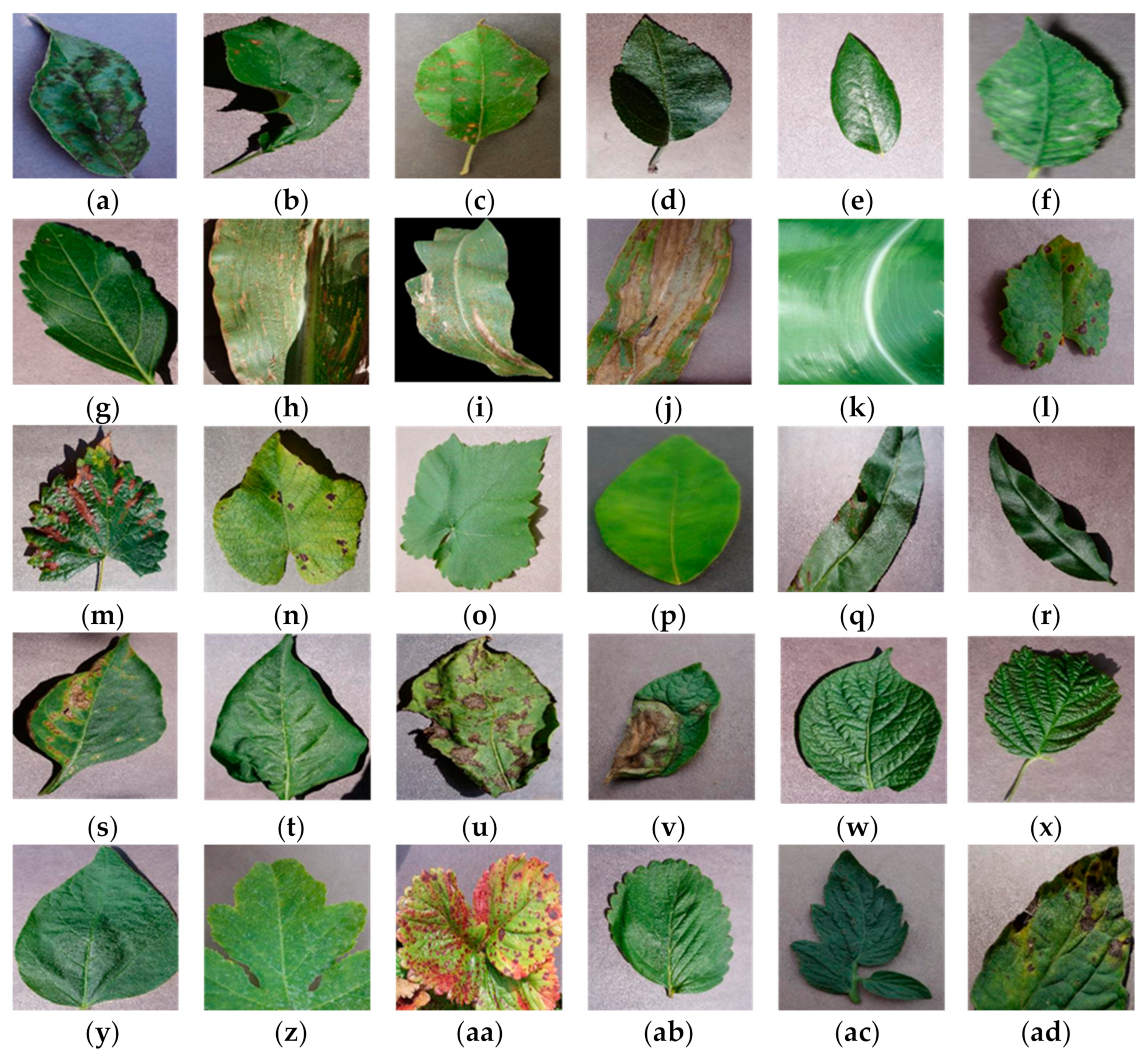
Figure 1. Sample images of PlantVillage dataset from each class. (a) Apple scab, (b) apple black rot, (c) cedar apple rust, (d) apple healthy, (e) blueberry healthy, (f) cherry powdery mildew, (g) cherry healthy, (h) corn gray leaf spot, (i) corn common rust, (j) corn northern leaf blight, (k) corn healthy, (l) grape block rot, (m) grape black measles, (n) grape leaf blight, (o) grape healthy, (p) orange healthy, (q) peach bacterial spot, (r) peach healthy, (s) pepper bacterial spot, (t) pepper healthy, (u) potato early blight, (v) potato late blight, (w) potato healthy, (x) raspberry healthy, (y) soybean healthy, (z) squash powdery mildew, (aa) strawberry leaf scorch, (ab) strawberry healthy, (ac) tomato bacterial spot, (ad) tomato early blight, (ae) tomato late blight, (af) tomato leaf mold, (ag) tomato septoria leaf spot, (ah) tomato spider mites, (ai) tomato target spot, (aj) tomato mosaic virus, (ak) tomato yellow leaf curl virus, and (al) tomato healthy.
Fractalfract 09 00691 g001aFractalfract 09 00691 g001b
Figure 2. Sample images of the Potato Leaf Disease dataset. (a) Early blight, (b) late blight, and (c) healthy.
Fractalfract 09 00691 g002
Figure 3. Example of low-light images. (a) Peach bacterial spot, (b) low-light peach bacterial spot, (c) low-light noisy peach bacterial spot, (d) potato late blight, (e) low-light potato late blight, and (f) low-light noisy potato late blight.
Fractalfract 09 00691 g003
Figure 4. Overall workflow of the proposed method.
Fractalfract 09 00691 g004
Figure 5. Overall structure of DPA-Net (LN means layer normalization).
Fractalfract 09 00691 g005
Figure 6. TDCB structure.
Fractalfract 09 00691 g006
Figure 7. FCB structure.
Fractalfract 09 00691 g007
Figure 8. MFEB structure.
Fractalfract 09 00691 g008
Figure 9. PAB structure.
Fractalfract 09 00691 g009
Figure 10. Accuracy and loss curves of training and validation by DPA-Net during training.
Fractalfract 09 00691 g010
Figure 11. Confusion matrix DPA-Net testing on PlantVillage (unit: %).
Fractalfract 09 00691 g011
Figure 12. Confusion matrix DPA-Net testing on the Potato Leaf Disease dataset (unit: %).
Fractalfract 09 00691 g012
Figure 13. Examples of poorly illuminated leaf images from (a) PlantVillage and (b) Potato Leaf Disease datasets.
Fractalfract 09 00691 g013
Figure 14. Grad-CAM visualization for the PlantVillage dataset. Correctly classified samples: original image, low-light noisy image, and Grad-CAM image from top to bottom, respectively. (a) Tomato spider mites, (b) corn northern leaf blight, (c) pepper bacterial spot, (d) tomato yellow leaf curl virus, and (e) peach bacterial spot.
Fractalfract 09 00691 g014
Figure 15. Grad-CAM visualization for the Potato Leaf Disease dataset. Correctly classified samples: original image, low-light noisy image, and Grad-CAM image from top to bottom, respectively. (a) Early blight, (b) late blight, and (c) healthy.
Fractalfract 09 00691 g015
Figure 16. FD analysis for the diseased and healthy leaves using activation map based on the predictions of DPA-Net: (a–d) from the left to right, Grad-CAM, their corresponding binarized image, and FD graph, respectively. (a) Healthy, and diseased cases of (b) black measles (orange class), (c) yellow leaf curl (tomato class), and (d) bacterial spot (pepper bell class).
Fractalfract 09 00691 g016
Figure 17. Misclassification of potato healthy as pepper healthy. (a) Potato healthy, (b) pepper healthy. The 1st and 2nd rows mean the original and corresponding low-light noisy images, respectively.
Fractalfract 09 00691 g017
Figure 18. Misclassification of potato late blight as potato early blight and potato healthy. (a) Potato healthy, (b) potato early blight, (c) potato late blight. The 1st and 2nd rows mean the original and corresponding low-light noisy images, respectively.
Fractalfract 09 00691 g018
Figure 19. Grad-CAM visualization for the PlantVillage dataset. Incorrectly classified samples: original image, low-light noisy image, Grad-CAM, and misclassified class image from top to bottom, respectively. (a) Tomato spider mite misclassified as tomato target spot, (b) corn northern leaf blight misclassified as corn common rust, (c) pepper bacterial spot misclassified as potato late blight, (d) tomato yellow leaf curl virus misclassified as orange healthy, and (e) peach bacterial spot misclassified as peach healthy.
Fractalfract 09 00691 g019
Figure 20. Grad-CAM visualization for the Potato Leaf Disease dataset. Incorrectly classified samples: original image, low-light noisy image, Grad-CAM, and misclassified class image from left to right, respectively. Early blight misclassified as late blight.
Fractalfract 09 00691 g020
Table 1. Comparisons of previous studies and the proposed method on the classification of plant diseases.
CategoryMethodDatasetClassesAccuracy (%)StrengthsLimitation
Using
handcrafted
features
EfficientNetB7 [6]PlantVillage479.23Early detection with less memory requirementsLow accuracy on untrained datasets
ELM [7]TPMD288.57Efficient for imbalanced dataset
-
Limited number of images in dataset
-
Works only for binary classes
Voting Classifier [8]PlantVillage392.60Improved accuracy with respect to SVMLimited to two classes of early and late blight diseases only
HSV + GLCM+ RF [9]Self-collected498High accuracy with less computational complexityLack of accuracy comparison
Using deep featuresUsing normal illumination imagesResNet-18 with transfer learning [12]Self-collected499.53High accuracy with fast processing speed
-
Do not detect multiple infections
-
Consider uniform illumination
ResNet-50 + MRDOA [13]PlantVillage1899.72
-
Optimized feature selection with reduced size MRDOA
-
Less training time
Require extensive preprocessing
Rice Plant dataset399.68
DenseNet + RGB Fusion [14]PlantVillage3898.17
-
Fast identification
-
Fusion shows higher accuracy as compared to single input
More training time and lack of hyperparameter optimization
MobileNet + VGG-16 with transfer learning [15]Self-collected589.2Outperform due to ensemble of DL models
-
System configuration is not specified
-
High number of trainable parameters
ResNet-34+ aECAnet [17]Peanut397.7
-
Robust generalization ability
-
Retain more channel information
-
No ablation study of attention module
-
Imbalanced data samples
PlantVillage3998.5
YOLO5 + PSA [18]Katra-twelve1298.25
-
Extract relevant features under complex background
-
Show higher performance than transformers
-
Complex diseases hinder correct classification
-
Model’s generality is compromised in pest identification
BARI-sunflower494.47
FGVC81293.55
GoogleNet + ECA [19]Self-collected899.58
-
Requires less computing power and parameters
-
Stable and highly accurate in the natural environment
High complexity of model
CNN + RCAB + FB [20]Self-collected599.95
-
Less processing time.
-
High flexibility of learning
-
Only valid to given classes
-
Not suitable for multiple diseases on a single leaf
ResNet-50 + ResNext blocks [21]New PlantVillage798.73
-
Computationally lighter and fast convergence
-
High generalization
-
Not effective for multi-disease detection
-
Limited to only the class of apple crop
MobileNet-V3 + ECA [22]Images from PlantVillage and PlantDoc 498.23
-
Requires fewer parameters and has high processing speed
-
Ideal for mobile devices
-
No consideration of field environment
-
Less variety of diseases
Using low-light noisy imagesDPA-Net (proposed)PlantVillage3892.11First study on plant disease classification of low-light noisy images Complex background is not considered
Potato Leaf Disease388.92
Table 2. Diseases and corresponding sample counts in the PlantVillage dataset.
Plant NameClass NameSampleTotal Number of Samples
AppleDiseaseScab6303171
Black rot621
Cedar apple rust275
Healthy1645
BlueberryHealthy15021502
CherryDiseasePowdery mildew 10521906
Healthy854
CornDiseaseGray leaf spot5133852
Common rust1192
Northern leaf blight985
Healthy1162
GrapeDiseaseBlack rot11804062
Black measles1383
Leaf blight1076
Healthy423
OrangeHealthy55075507
PeachDiseaseBacterial spot 22972657
Healthy360
PepperDiseaseBacterial spot9972475
Healthy1478
PotatoDiseaseEarly blight10002152
Late blight1000
Healthy152
RaspberryHealthy371371
SoybeanHealthy50905090
SquashDiseasePowdery mildew18351835
StrawberryDiseaseLeaf scorch11091565
Healthy456
TomatoDiseaseBacterial spot212718,160
Early blight1000
Late blight1909
Leaf mold952
Septoria leaf spot1771
Spider mites1676
Target spot1404
Mosaic virus373
Yellow leaf curl virus5357
Healthy1591
Total number of images54,305
Table 3. Diseases and corresponding sample counts in the Potato Leaf Disease dataset.
Plant NameClass NameTotal Number of Samples
PotatoDiseaseEarly blight1628
Late blight1424
Healthy1020
Total number of images4072
Table 4. Performance comparisons with or without the proposed blocks (unit: %).
CaseDCBFCBMFEBPABAccuracyPrecisionRecallF1-Score
1 89.8486.9785.5486.25
2 90.7988.0686.9487.49
3 90.8988.2687.0287.63
4 90.2287.2586.3286.78
5 90.3687.6186.3686.98
6 91.1788.6487.1887.90
7 91.5489.1587.8888.51
Proposed (DPA-Net)92.1189.7388.4989.11
Table 5. Performance comparisons with different dilation rates for the TDCB (unit: %).
Dilation RateAccuracyPrecisionRecallF1-Score
1, 2, 491.5188.9487.8988.41
1, 4, 691.5489.2287.8488.52
1, 3, 5 (proposed)92.1189.7388.4989.11
Table 6. Performance comparisons with different number of layers in the TDCB (unit: %).
Dilation LayersDilate RateAccuracyPrecisionRecallF1-Score
23, 591.6789.2388.2188.72
3 (proposed)1, 3, 592.1189.7388.4989.11
41, 3, 5, 791.8489.5388.2788.89
Table 7. Performance comparisons according to layers and fusions in the FCB (unit: %).
MethodAccuracyPrecisionRecallF1-Score
With 3 × 3 convolution layer only91.8889.2388.3288.77
With 1 × 1 convolution layer only91.6689.0387.9888.50
Without attention92.0489.7388.4789.10
With attention (proposed)92.1189.7388.4989.11
Table 8. Performance comparisons according to various parallel layers of the MFEB (unit: %).
MethodAccuracyPrecisionRecallF1-Score
Without A91.9189.2088.3388.76
Without B91.9489.4988.3688.92
Without C91.9989.8788.3389.09
Without F291.5488.9387.9788.38
With A, B, C, and F2 (proposed)92.1189.7388.4989.11
Table 9. Performance comparison on hyperparameter sensitivity for the Potato Leaf Disease dataset.
CaseLearning RateBatch SizeAccuracyPrecisionRecallF1-Score
10.00005868.1067.6567.3967.52
20.0005863.8867.3163.1065.14
30.00011676.3176.0575.8475.94
40.0001479.0178.6378.6178.62
Proposed0.0001888.9288.8888.3288.60
Table 10. Performance comparisons of DPA-Net with different SOTA methods on the PlantVillage dataset (unit: %).
MethodAccuracyPrecisionRecallF1-Score
Swin-T [43]69.1360.7759.8960.32
SqueezeNet [44]76.7272.3467.8070.00
ShuffleNet [45]76.9670.9666.7768.79
AlexNet [46]81.1474.7975.0874.93
XceptionNet [47]88.0083.9083.4183.65
Resnet-50 [48]88.1284.0783.9484.01
MobileNet-V2 [49]88.6184.9484.2184.57
VGG-16 [50]88.9585.5884.5885.08
InceptionNet [51]89.4085.8985.7085.80
DenseNet-121 [52]89.6386.0785.6885.87
ConvNext-small [53]89.8486.9785.5486.25
DPA-Net (proposed)92.1189.7388.4989.11
Table 11. Performance comparisons of DPA-Net with different SOTA methods on the Potato Leaf Disease dataset (unit: %).
MethodAccuracyPrecisionRecallF1-Score
Swin-T [54]39.9413.1133.3319.03
SqueezeNet [55]54.0755.9449.1551.60
ShuffleNet [56]66.5566.4765.2665.85
AlexNet [57]43.0825.7236.7528.18
XceptionNet [58]71.3071.0970.5270.80
ResNet-50 [59]78.1378.3677.3677.85
MobileNet-V2 [60]73.5373.5872.4973.02
VGG-16 [61]75.6475.6975.2175.44
InceptionNet [62]75.7074.8075.0574.93
DenseNet-121 [63]77.5977.1877.1077.14
EfficientNetV2 [64]78.8778.5677.8078.18
ConvNext-small [65]82.6082.6381.8682.23
DPA-Net (proposed)88.9288.8888.3288.60
Table 12. Complexity comparisons of DPA-Net with different SOTA methods on PlantVillage dataset.
Method#Param (M)FLOPs (G)Memory Usage (MB)
Swin-T [43]18.892.9872.03
SqueezeNet [44]0.750.742.88
ShuffleNet [45]0.380.041.45
AlexNet [46]57.160.71218.05
XceptionNet [47]20.894.6079.67
Resnet-50 [48]23.594.1389.97
MobileNet-V2 [49]2.270.338.67
VGG-16 [50]134.4215.52512.79
InceptionNet [51]25.195.7596.09
DenseNet-121 [52]6.992.9026.68
ConvNext-small [53]49.448.68188.61
DPA-Net (proposed)52.359.63199.72
Table 13. Complexity comparison of DPA-Net with different SOTA methods on the Potato Leaf Disease dataset.
Method#Param (M)FLOPs (G)Memory Usage (MB)
Swin-T [54]18.852.9871.92
SqueezeNet [55]0.740.732.81
ShuffleNet [56]0.340.041.32
AlexNet [57]57.020.71217.50
XceptionNet [58]20.814.6079.40
ResNet-50 [59]23.514.1389.70
MobileNet-V2 [60]2.230.338.50
VGG-16 [61]134.2815.52512.24
InceptionNet [62]25.115.7595.82
DenseNet-121 [63]6.962.9026.54
EfficientNetV2 [64]20.188.3776.99
ConvNext-small [65]49.418.68188.50
DPA-Net (Proposed)52.339.63199.61
Table 14. Comparison of processing times in DPA-Net and SOTA methods (unit: ms).
MethodDesktop ComputerJetson TX2
Swin-T [43]5.69606.65
SqueezeNet [44]4.2611.28
ShuffleNet [45]4.9610.87
AlexNet [46]4.158.58
XceptionNet [47]5.0629.92
Resnet-50 [48]5.0831.26
MobileNet-V2 [49]4.7311.82
VGG-16 [50]8.284.61
InceptionNet [51]7.755.51
DenseNet-12 [52]6.6729.61
ConvNext-small [53]9.6389.55
DPA-Net (proposed)10.2696.29
Table 15. Robustness to the illumination and noise level for Potato Leaf Disease dataset.
S γ σ AccuracyPrecisionRecallF1-Score
1.50.52488.4088.4988.0188.25
1.50.52688.4788.2088.4888.34
1.40.52587.9887.8087.5587.67
1.60.52589.3889.3688.8789.11
1.50.52588.9288.8888.3288.60
1.50.62589.5189.8089.1789.48
Table 16. Performance of DPA-Net on real low-illumination dataset.
AccuracyPrecisionRecallF1-Score
85.0086.2685.0085.63
Table 17. Comparative analysis of FD, R2, and C for diseased and healthy cases.
ResultsHealthy CaseDisease Cases
Black MeaslesYellow Leaf CurlBacterial Spot
FD1.64531.24861.26621.2748
R20.99780.99040.99000.9916
C0.99890.99520.99500.9958
Table 18. Performance comparisons of DPA-Net with and without FD analysis on the Potato Leaf Disease dataset (unit: %).
MethodAccuracyPrecisionRecallF1-Score
DPA-Net (proposed)88.9288.8888.3288.60
DPA-Net (proposed) with FD analysis93.6896.7595.0795.86
Disclaimer/Publisher’s Note: The statements, opinions and data contained in all publications are solely those of the individual author(s) and contributor(s) and not of MDPI and/or the editor(s). MDPI and/or the editor(s) disclaim responsibility for any injury to people or property resulting from any ideas, methods, instructions or products referred to in the content.