Abstract
This paper is concerned with the global funnel control (FC) issue of the nonlinear systems with unknown dynamics and time-varying fractional powers. An FC strategy is proposed in this paper, not only the barrier functions but also the tracking and intermediate errors are introduced to our control law in a proportional feedback way, which not only guarantees uniform performance insurance under any initial condition of the control system but also leads to about 50% reduction in control amplitude with respect to the existing solutions. Moreover, it exhibits notable simplicity, with no need for parametric details of time-varying fractional powers, adding a power integrator technique, parameter identification, function approximation or derivative calculation. A comparative simulation demonstrates the effectiveness and superiority of the developed method.
1. Introduction
Given the theoretical difficulties and practical demands, considerable research attention has been devoted to the control of the uncertain nonlinear systems involving fractional powers. In engineering contexts, such odd-power nonlinear systems can be found in various applications, with under-actuated mechanical systems [1] and dynamical boiler–turbine units [2] being typical instances. Notably, feedback linearization fails to be applied to this type of system, which stems from the uncontrollability of its Jacobian matrix. Additionally, the system exhibits a nonaffine relationship with the control input. As a result, formulating control strategies for odd-power systems poses significant challenges. To deal with this problem, a variety of methods have been proposed, such as adaptive [3,4,5,6,7,8,9], neural or fuzzy control [10,11,12], adding a power integrator technique [9,13,14,15,16], and funnel or prescribed performance control [11,12,17]. Nevertheless, the application scope of the aforementioned approaches is confined to integer powers. In contrast, some schemes for the control systems involving fractional powers have been developed recently [5,6,8,17,18,19,20]. In the literature [18,19], the fractional powers greater than zero and less than one are taken into consideration. It is important to highlight that a shared characteristic of the above-mentioned results is the requirement for known powers. Notably, the power integrator addition technique proves unsuitable for scenarios involving unknown powers, as it depends heavily on the homogeneous dominant component. To handle this situation, numerous approaches were put forward in the literature [9,14,15,16], but the bounds of powers need to be available for the control design. Additionally, the system nonlinearities of the aforementioned results are either constrained by known functions [1,4,7,13] or represented by a structure featuring both known functions and unknown parameters [9,16].
FC aims at fast and accurate reference tracking, with both the settling time and accuracy less than the respectively preselected values. This is accomplished by restricting the tracking error within a preselected performance boundary. In the conventional performance design, however, the choice of performance functions is contingent upon the initial condition of the control system [11,12,17,21,22,23,24,25,26]. Once the initial error is outside the performance envelope, the control signal becomes insolvable (e.g., ) or leads to a positive feedback loop. As a result, only semi-global performance of the control system is able to be ensured. For global FC, a predefined-time tuning function is designed to modify the tracking and intermediate errors within the FC framework [27]. By this means, the issue of global, fast and accurate convergence for all errors is converted into the problem of local constraints of the adjusted errors that can be addressed by using the barrier function-based control approach. Alternatively, employing a shifting function and a performance function where the initial value approaches infinity is also effective [28,29,30,31,32,33]. Nevertheless, the existing global FC methods work for the standard strict-feedback systems without fractional powers [27,28,29,30,31]. In addition to this, extensive simulation and experimental results show that the above global FC methods yield large control amplitude during the transient phase (e.g., control peak) when there is a large initial error. Due to actuator saturation of the practical control system, the performance requirement may not hold. Additionally, global stability can also be guaranteed by other control methods, e.g., the improved adaptive control [9,29,30,31,34,35,36,37], neural network control [32,38] and small-gain theorem [35]. Unfortunately, they are applicable to the standard strict-feedback systems [27,28,29,30,31,32,33,34,36]; they can assume the parametrically uncertain nonlinearities or their bounding functions [9,29,30,31,34,36]; they involve sign functions in the control law [34,36]. The theoretical comparison is shown in Table 1.

Table 1.
Theoretical comparison.
The above discussion reveals that the global FC problem of the nonlinear systems with unknown, time-varying, and fractional powers remains open. To this end, a novel FC strategy is designed in this paper. Its superiority is enumerated as follows.
- It is effective for the nonlinear systems with unknown, time-varying, fractional powers and totally unknown closed-loop dynamics, in contrast to the references [1,4,7,8,9,10,11,12,13,14,15,16,27,28,29,30,31,32,33,34].
- It shows flexibility in the sense of the global performance insurance, the continuous control input, and the reduced control amplitude, with respect to the results [9,13,20,21,22,23,24,25,26].
- The simplicity of FC is preserved, without needs for parameter identification [4,5,6,7,8], adding a power integrator technique [9,14,15,16], function approximation [10,11,12] or derivative calculation [31,33].
2. Problem Formulation
2.1. System Description
Consider the following nonlinear system with time-varying fractional powers:
where ; constitutes the system state; is a continuous and time-varying scalar of which the scope covers both the integer and the fraction, ; and are the input and the output, respectively; the power sign function is defined as for a real number ; , , are the nonlinear functions, each of which is continuous in their respective arguments.
Assumption 1.
There are constants, and , for which the following is true:
2.2. Control Objective
The control objective for (1) is to drive to track , with the following:
where , , and are the preselected positive constants with ; denotes the initial value of (i.e., ); denotes the largest acceptable deviation of the steady-state error; denotes the expected rate at which the performance boundary decreases from to ; denotes the expected settling time of reference tracking.
Assumption 2.
Both and are bounded over [10,18,21,22,23,27].
Remark 1.
This study is concentrated on the case where neither the specific knowledge of the nonlinear dynamics in (1) nor the bound of time-varying fractional powers in Assumption 1 and the bound of the reference derivative in Assumption 2 are available for the control design below.
To summarize, the problem investigated herein is summarized below.
3. Control Development
A predefined-time tuning function is employed:
where is given in (3). Adopt it to modify the tracking error:
For any and , we know from (4) and (5) that the following is true:
Based on (4), the tracking performance requirement in (3) is transformed to the following:
On the purpose of (8), we employ a barrier function:
which yields the first intermediate control law:
where and are free-design constants, standing for the virtual control gains. We now advance to the following:
for , recursively, where , , and are the freely-chosen constants. Ultimately, the control law is acquired by the following:
The block diagram of the system with the controller is given in Figure 1.
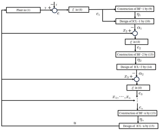
Figure 1.
The block diagram of the system with the controller.
Remark 2.
Different from the existing global FC laws [23,24,25,26], not only the barrier functions but also the tracking and intermediate errors are introduced to our control law in a proportional feedback way. By this means, the task of errors stabilization is divided into the barrier functions and errors together, i.e., the feedback errors share partial responsibility. The simulation results below show the significant advantage of the amended FC law in reduction of the control amplitude, especially during the transient phase of the control system.
4. Performance Analysis
Lemma 1.
For any and , , we obtain the following:
Proof.
Substituting (6) into (9) with (3) yields the following:
Putting (6) and (18) into (10), one has the following:
By (4) and (11), the following is obtained:
Substituting it into (13) with (12) yields the following:
Putting (20) and (21) into (14), one has the following:
From (4), (11) and (22), there holds the following:
Continue along the same path to examine , , one by one. We are able to conclude the following:
for . Based on (15), (17) holds. □
Lemma 2.
For any and each , during , provided
- evolves inside and keeps at a distance from and during ;
- and are both bounded during .
Proof.
The derivatives of (9) and (13) are computed by the following:
Differentiating (10) and (14) gives the following:
Substituting (27) into (29) yields the following:
It follows from (3) and (12) that and are bounded, . The boundedness of in (9) and (13) guarantees that of in (28), . Therefore, on under the assumed conditions of Lemma 2, . □
Lemma 3.
Under (4), consider a continuous scalar function with bounded . Firstly, for any , if the following is true:
then
Secondly, for any , if the following is true:
then
Proof.
We show (32) and (34) by contradiction. At the outset, suppose (31) but with the following:
This means that , which in turn indicates from (4) that . As a result, (31) is rephrased by the following:
However, is bounded, which contradicts (36). Hence, (35) is invalid, and instead, (32) is established. Suppose (33) but there is for which the following is true:
By (33) and (37), we further have the following:
which in turn implies from (4) that . Thus, (37) is rewritten by the following:
which however contradicts the fact that . Thereby, (37) is invalid, and instead, (34) is true. □
Theorem 1.
Proof.
We commence with the argument that the following is true:
for . This assertion is validated using the proof by contradiction method. From (3) and (12), we have , , which in conjunction with Lemma 1 give (40) at . Note that , , in (1) and , , in (3) and (12) are all uniformly continuous. The uniform continuity of follows from (4) and Assumption 2. Thus, the continuity of in (9) and in (10) is guaranteed, if . Further, the continuity of in (11) holds under the identical condition. Continuing along the same path to examine , , one by one, we are able to conclude that is continuous in the case of , . These findings indicate that a violation of (40) implies the existence of for which the following is true:
with
Next, (41) with (42) is supposed, and each case in (41) is to be enumerated for verification. For brevity, the arguments of some functions may not be shown.
Case 1: Initially, we examine the following:
Under (42), a precondition for (43) is the following:
Differentiating (5) by (1) yields the following:
where
This further holds the following:
It follows from Assumption 2 and Equation (4) that , , , and are bounded. From (42), one has , , . By the second item of Lemma 3, there holds over , which in turn warrants (i.e., ) on . Due to the continuity of in , we have , . Inserting these findings into (46) gives the following:
Note from (9) and (43) that the following is true:
Under (10), there further holds the following:
Applying the first item of Lemma 3 to (50) yields the following:
By (11), we have the following:
Further, there holds the following:
Putting (51) into (53) under (42) yields the following:
By (4), there holds the following:
It further follows that the following is true:
Further, substituting (48) and (56) into (47) shows the following:
Note from (3) that is bounded. Apparently, (57) contradicts (44). Therefore, (43) is invalid. There instead exists a constant, , for which the following is true:
Consequently, in (9) and in (10) remain bounded on . Under (11) and (42), invoking the second item of Lemma 3 yields is bounded on , which implies that , . By (45), during . This in company with (58) yields by Lemma 2 that over .
Case 2: Consider the following:
Under (42), a precondition for (59) is the following:
Taking the derivative of in (11) via (1), we have the following:
where
Further, there holds the following:
Note that , , , , and are all bounded during . Since is continuous with respect to , we further have , . Putting the above facts into (62) leads to the following:
One sees from (13) and (59) that the following is true:
By (14), there further holds the following:
Applying the first item of Lemma 3 to (66) yields the following:
From (11), we have the following:
Further, there holds the following:
Putting (67) into (69) under (42) yields the following:
By (4), there holds the following:
It further follows that the following is true:
Further, substituting (64) and (72) into (63) shows the following:
Note from (12) that is bounded. Obviously, (73) contradicts (60). Hence, (59) is invalid. There instead is a constant, , for which the following is true:
Further, in (13) and in (14) are bounded over . Under (11) and (42), invoking the second item of Lemma 3 yields is bounded on , which implies that , . By (61), is bounded over . This in conjunction with (74) yields by Lemma 2 that on .
Case i (): Adopting the same analytical way from Case 2, we can conclude that there are a set of positive constants, , for which the following is true:
Clearly, (58), (74) and (75) contradict (41). Therefore, (41) is invalid. There instead holds the following:
It is apparent that the claim in (40) is valid. This shows that the controller warrants the error constraints but evades the errors approaching the preselected boundaries. Further, it follows from (4), (5) and (40) for that (3) is established.
It remains for us to verify that the rest of the signals in the closed loop are bounded. From (9), (13) and (76), there hold for , . This in conjunction with (10), (14), (15) and (40) ensures the uniform boundedness of and u, . Based on (5), (11), (40) and the second item of Lemma 3, there hold and for , . By Assumption 2, there further hold , , are bounded for . □
Remark 3.
The proof by contradiction reveals the inherent robustness of the developed control approach to the unknown nonlinearities and time-varying fractional powers. This phenomenon results from the infinity property of the barrier functions, as shown in (55) and (71). When extended to the nonlinear system with unknown powers in (1), the infinity property remains preserved, as indicated in (56) and (72). Therefore, only a bounded control input is needed, the techniques for approximation, identification and estimation are removed.
5. Simulation Study
To evaluate the proposed control strategy, a comparative simulation study is conducted.
Case 1: Consider the following second-order systems with time-varying fractional powers:
In the simulation, (77) is initialized at either or . The control task is to driver to follow with the following:
The design of the controller follows from Theorem 1 with , , , , and . Applying it to (77), Figure 2, Figure 3, Figure 4, Figure 5 and Figure 6 illustrate the simulation results. As depicted in Figure 2 and Figure 3, the output follows the reference under varying initial values, and the tracking error achieves convergence to the designated performance envelope within the predefined duration. Thereby, under different initial conditions, the prescribed performance specification in (78) is implemented, which implies the global attribute. Similarly, the preassigned performance specification for the intermediate error is also fulfilled, as displayed in Figure 4. Finally, one sees from Figure 5 and Figure 6 that both the other state variable and the input are bounded under different initial conditions. Accordingly, the simulation findings confirm the effectiveness of the developed controller.
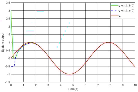
Figure 2.
The system output under and .
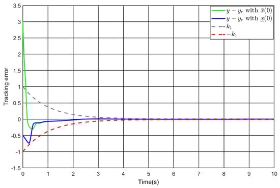
Figure 3.
The tracking error under and .
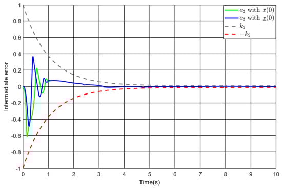
Figure 4.
The intermediate error under and .
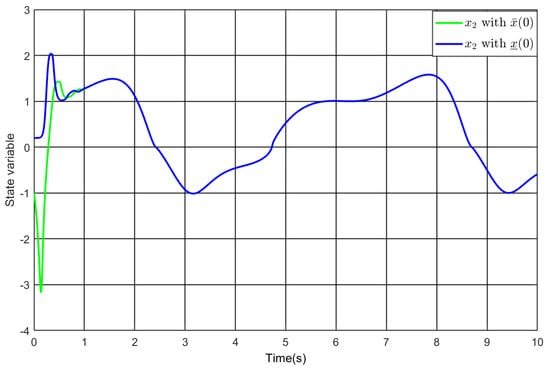
Figure 5.
The state variable under and .
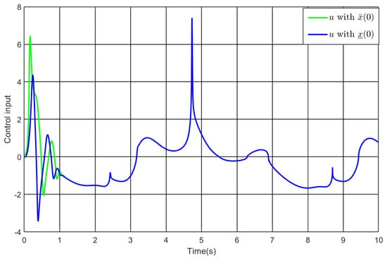
Figure 6.
The control input under and .
For comparison, an enhancing prescribed performance control scheme is implemented for (77) under the identical control task. The controller is designed by [39] as follows:
Take into consideration. Figure 7, Figure 8, Figure 9 and Figure 10 exhibit the simulation findings. Despite ensuring that the control system achieves predefined performance and all signals remain bounded, the comparative controller demands that the nonlinearity is known and that the first and second-order derivatives of the reference are obtainable. Moreover, the choice of performance boundaries is contingent upon the initial condition of the control system. In contrast, the above requirements are eliminated by our approach. In addition, the comparative controller requires larger amplitude of the control input. To be specific, Figure 10 shows with the comparative controller and with our controller. Thus, the comparative simulation findings illustrate the advantage of the developed strategy. The performance comparison between different controllers is given in Table 2.
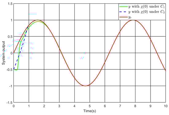
Figure 7.
The system output under our controller and the comparative controller .
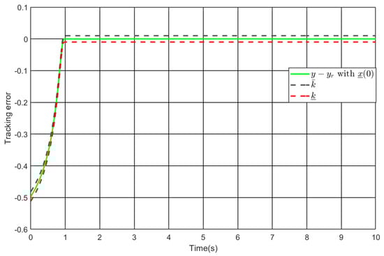
Figure 8.
The tracking error under the comparative controller .
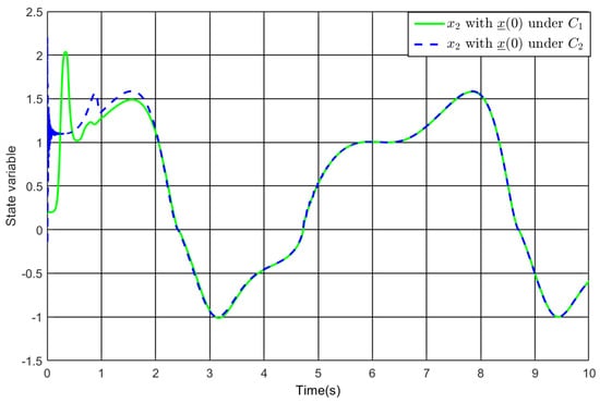
Figure 9.
The state variable under our controller and the comparative controller .
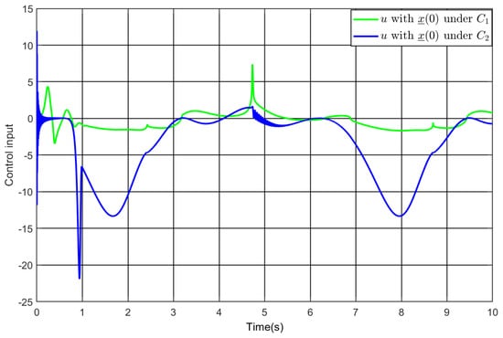
Figure 10.
The control input under our controller and the comparative controller .
Table 2.
Performance comparison between different controllers under .
To enrich the comparison, a conventional PI controller is designed below and applied to (77) under the same initial conditions:
where , , and . The simulation results are given in Figure 11 and Figure 12. It is observed that the tracking performance is clearly inadequate, with the tracking error going beyond the predefined performance boundary. As such, the comparative simulation results confirm the superiority of the control strategy proposed in this study.
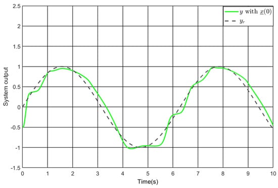
Figure 11.
The system output under PI control.
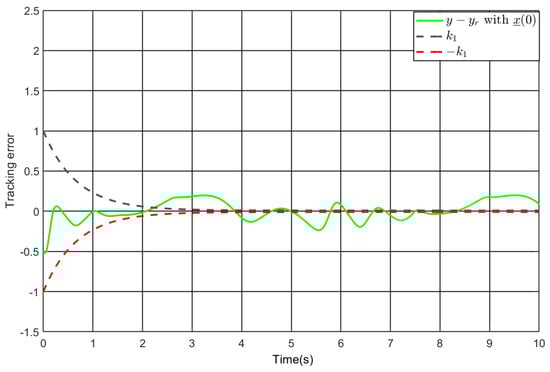
Figure 12.
The tracking error under under PI control.
Case 2: Consider the following second-order systems with time-varying fractional powers [27]:
with , and . In the simulation, (80) is initialized at either or . The control task is to driver to follow with the following:
The design of the controller follows from Theorem 1 with , , , , , and . Applying it to (80), Figure 13, Figure 14 and Figure 15 illustrate the simulation results. As depicted in Figure 13 and Figure 14, the output follows the reference under varying initial values, and the tracking error achieves convergence to the designated performance envelope within the predefined duration. Finally, one sees from Figure 15 that the input are bounded under different initial conditions. Accordingly, the simulation findings confirm the generality of the developed controller.
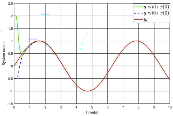
Figure 13.
The system ouput under and .
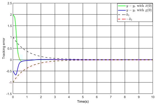
Figure 14.
The tracking error under and .
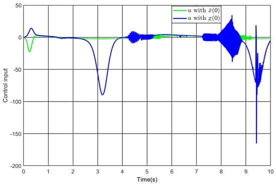
Figure 15.
The control input under and .
6. Conclusions
We put forward an FC approach for reference tracking with prescribed performance in this paper. It is able to cope with unknown nonlinearities and unknown time-varying fractional powers. It achieves fast accurate reference tracking under arbitrary initial state of the control system and removes the requirements for specific information of the time-varying fractional powers, the parametrically uncertain form of system dynamics and the tools for approximation, identification and estimation. Moreover, the required control input is both continuous and shows lower amplitude than the conventional global FC laws. The simulation results validate our approach. Subsequent research will address robustness to measurement noise, bounded disturbances, and actuator saturation in real applications.
Author Contributions
Conceptualization, R.-B.G. and X.Z.; methodology, R.-B.G. and X.Z.; validation, R.-B.G.; formal analysis, R.-B.G.; investigation, R.-B.G. and X.Z.; writing-original draft preparation, R.-B.G.; writing—review and editing, X.Z., V.A. and H.-S.A.; vsualization, R.-B.G.; supervision, X.Z.; funding acquisition, X.Z. All authors have read and agreed to the published version of the manuscript.
Funding
This work was supported in part by the National Natural Science Foundation of China under Grant 62103093, the National Key Research and Development Program of China under Grant 2022YFB3305905, the Fundamental Research Funds for the Central Universities under Grant N2224005-3 and the National Key Research and Development Program Topic under Grant 2020YFB1710003.
Data Availability Statement
No new data were created or analyzed in this study. Data sharing is not applicable to this article.
Conflicts of Interest
The authors declare no conflicts of interest.
References
- Xie, X.J.; Duan, N. Output tracking of high-order stochastic nonlinear systems with application to benchmark mechanical system. IEEE Trans. Autom. Control 2010, 55, 1197–1202. [Google Scholar]
- Liu, J.Z.; Yan, S.; Zeng, D.L.; Hu, Y.; Lv, Y. A dynamic model used for controller design of a coal fired once-through boiler-turbine unit. Energy 2015, 93, 2069–2078. [Google Scholar] [CrossRef]
- Zhang, X.; Liu, R.; Ren, J.; Gui, Q. Adaptive Fractional Image Enhancement Algorithm Based on Rough Set and Particle Swarm Optimization. Fractal Fract. 2022, 6, 100. [Google Scholar] [CrossRef]
- Xie, X.J.; Tian, J. Adaptive state-feedback stabilization of high-order stochastic systems with nonlinear parameterization. Automatica 2009, 45, 126–133. [Google Scholar] [CrossRef]
- Li, W.; Jing, Y.; Zhang, S. Adaptive state-feedback stabilization for a large class of high-order stochastic nonlinear systems. Automatica 2011, 47, 819–828. [Google Scholar] [CrossRef]
- Li, W.; Liu, X.; Zhang, S. Further results on adaptive state-feedback stabilization for stochastic high-order nonlinear systems. Automatica 2012, 48, 1667–1675. [Google Scholar] [CrossRef]
- Liu, L.; Yin, S.; Gao, H.; Alsaadi, F.; Hayat, T. Adaptive partial-state feedback control for stochastic high-order nonlinear systems with stochastic input-to-state stable inverse dynamics. Automatica 2015, 51, 285–291. [Google Scholar] [CrossRef]
- Sun, Z.Y.; Xue, L.R.; Zhang, K. A new approach to finite-time adaptive stabilization of high-order uncertain nonlinear system. Automatica 2015, 58, 60–66. [Google Scholar] [CrossRef]
- Man, Y.; Liu, Y. Global adaptive stabilization and practical tracking for nonlinear systems with unknown powers. Automatica 2019, 100, 171–181. [Google Scholar] [CrossRef]
- Ma, J.; Wang, H.; Su, Y.; Liu, C.; Chen, M. Adaptive neural fault-tolerant control for nonlinear fractional-order systems with positive odd rational powers. Fractal Fract. 2022, 6, 622. [Google Scholar] [CrossRef]
- Wang, N.; Wang, Y. Fuzzy adaptive quantized tracking control of switched high-order nonlinear systems: A new fixed-Time prescribed performance method. IEEE Trans. Circuits Syst. II Exp. Briefs 2022, 69, 3279–3283. [Google Scholar] [CrossRef]
- Fu, Z.; Wang, N.; Song, S.; Wang, T. Adaptive fuzzy finite-Time tracking control of stochastic high-order nonlinear systems with a class of prescribed performance. IEEE Trans. Fuzzy Syst. 2022, 30, 88–96. [Google Scholar] [CrossRef]
- Lin, W.; Qian, C. Adding one power integrator: A tool for global stabilization of high-order lower-triangular systems. Syst. Control Lett. 2000, 39, 339–351. [Google Scholar] [CrossRef]
- Chen, C.C.; Qian, C.; Lin, X.; Sun, Z.Y.; Liang, Y.W. Smooth output feedback stabilization for a class of nonlinear systems with time-varying powers. Int. J. Robust Nonlinear Control 2017, 27, 5113–5128. [Google Scholar] [CrossRef]
- Su, Z.; Qian, C.; Shen, J. Interval homogeneity-based control for a class of nonlinear systems with unknown power drifts. IEEE Trans. Autom. Control 2017, 62, 1445–1450. [Google Scholar] [CrossRef]
- Xie, X.J.; Guo, C.; Cui, R.H. Removing feasibility conditions on tracking control of full-State constrained nonlinear systems with time-varying powers. IEEE Trans. Syst. Man Cybern. Syst. 2021, 51, 6535–6543. [Google Scholar] [CrossRef]
- Zhang, L.; Liu, X.; Hua, C. Prescribed-time control for stochastic high-order nonlinear systems with parameter uncertainty. IEEE Trans. Circuits Syst. II Exp. Briefs 2023, 70, 4083–4087. [Google Scholar] [CrossRef]
- Lv, M.; De Schutter, B.; Cao, J.; Baldi, S. Adaptive prescribed performance asymptotic tracking for high-order odd-rational-power nonlinear systems. IEEE Trans. Autom. Control 2023, 68, 1047–1053. [Google Scholar] [CrossRef]
- Sui, S.; Chen, C.L.P.; Tong, S. Finite-time adaptive fuzzy prescribed performance control for high-order stochastic nonlinear systems. IEEE Trans. Fuzzy Syst. 2022, 30, 2227–2240. [Google Scholar] [CrossRef]
- Zhao, C.R.; Xie, X.J. Global stabilization of stochastic high-order feedforward nonlinear systems with time-varying delay. Automatica 2014, 50, 203–210. [Google Scholar] [CrossRef]
- Chowdhury, D.; Khalil, H.K. Funnel control for nonlinear systems with arbitrary relative degree using high-gain observers. Automatica 2019, 105, 107–116. [Google Scholar] [CrossRef]
- Dimanidis, I.S.; Bechlioulis, C.P.; Rovithakis, G.A. Output feedback approximation-free prescribed performance tracking control for uncertain MIMO nonlinear systems. IEEE Trans. Autom. Control 2020, 65, 5058–5069. [Google Scholar] [CrossRef]
- Bechlioulis, C.P.; Rovithakis, G.A. Robust partial-state feedback prescribed performance control of cascade systems with unknown nonlinearities. IEEE Trans. Autom. Control 2011, 56, 2224–2230. [Google Scholar] [CrossRef]
- Zhang, J.X.; Ding, J.; Chai, T. Cyclic performance monitoring-based fault-tolerant funnel control of unknown nonlinear systems with actuator failures. IEEE Trans. Autom. Control 2025, 70, 6111–6118. [Google Scholar] [CrossRef]
- Zhang, J.X.; Yang, G.H. Low-complexity tracking control of strict-feedback systems with unknown control directions. IEEE Trans. Autom. Control 2019, 64, 5175–5182. [Google Scholar] [CrossRef]
- Zhang, J.X.; Liu, Y.Q.; Chai, T. Singularity-free low-complexity fault-tolerant prescribed performance control for spacecraft attitude stabilization. IEEE Trans. Autom. Sci. Eng. 2025, 22, 15408–15419. [Google Scholar] [CrossRef]
- Zhang, J.X.; Yang, G.H. Robust Adaptive fault-tolerant control for a class of unknown nonlinear systems. IEEE Trans. Ind. Electron. 2017, 64, 585–594. [Google Scholar] [CrossRef]
- Zhang, J.X.; Yang, G.H. Adaptive asymptotic stabilization of a class of unknown nonlinear systems with specified convergence rate. Int. J. Robust Nonlinear Control 2019, 29, 238–251. [Google Scholar] [CrossRef]
- Song, Y.D.; Zhou, S. Tracking control of uncertain nonlinear systems with deferred asymmetric time-varying full state constraints. Automatica 2018, 98, 314–322. [Google Scholar] [CrossRef]
- Zhou, S.; Song, Y.; Luo, X. Fault-tolerant tracking control with guaranteed performance for nonlinearly parameterized systems under uncertain initial conditions. J. Frankl. Inst. 2020, 357, 6805–6823. [Google Scholar] [CrossRef]
- Zhao, K.; Song, Y.; Chen, C.L.P.; Chen, L. Adaptive asymptotic tracking with global performance for nonlinear systems with unknown control directions. IEEE Trans. Autom. Control 2022, 67, 1566–1573. [Google Scholar] [CrossRef]
- Zhao, K.; Chen, L.; Chen, C.L.P. Event-based adaptive neural control of nonlinear systems with deferred constraint. IEEE Trans. Syst. Man Cybern. Syst. 2022, 52, 6273–6282. [Google Scholar] [CrossRef]
- Berger, T.; Lê, H.H.; Reis, T. Funnel control for nonlinear systems with known strict relative degree. Automatica 2018, 87, 345–357. [Google Scholar] [CrossRef]
- Wang, Y.; Liu, Y. Global practical tracking via adaptive output feedback for uncertain nonlinear systems without polynomial constraint. IEEE Trans. Autom. Control 2021, 66, 1848–1855. [Google Scholar] [CrossRef]
- Jiang, Z.P.; Mareels, I.; Hill, D.; Huang, J. A unifying framework for global regulation via nonlinear output feedback: From ISS to iISS. IEEE Trans. Autom. Control 2004, 49, 549–562. [Google Scholar] [CrossRef]
- Chen, W.; Wen, C.; Wu, J. Global exponential/finite-time stability of nonlinear adaptive switching systems with applications in controlling systems with unknown control direction. IEEE Trans. Autom. Control 2018, 63, 2738–2744. [Google Scholar] [CrossRef]
- Liu, L.; Huang, J. Global robust stabilization of cascade-connected systems with dynamic uncertainties without knowing the control direction. IEEE Trans. Autom. Control 2006, 51, 1693–1699. [Google Scholar] [CrossRef]
- Zhou, Y.; Zhou, Y.; Wan, P. Prescribed finite-time stabilization of fuzzy neural networks with time-varying controller. J. Autom. Intell. 2024, 3, 176–184. [Google Scholar] [CrossRef]
- Shi, Y.; Yi, B.; Xie, W.; Zhang, W. Enhancing prescribed performance of tracking control using monotone tube boundaries. Automatica 2024, 159, 111304. [Google Scholar] [CrossRef]
Disclaimer/Publisher’s Note: The statements, opinions and data contained in all publications are solely those of the individual author(s) and contributor(s) and not of MDPI and/or the editor(s). MDPI and/or the editor(s) disclaim responsibility for any injury to people or property resulting from any ideas, methods, instructions or products referred to in the content. |
© 2025 by the authors. Licensee MDPI, Basel, Switzerland. This article is an open access article distributed under the terms and conditions of the Creative Commons Attribution (CC BY) license (https://creativecommons.org/licenses/by/4.0/).