Outlier-Robust Convergence of Integer- and Fractional-Order Difference Operators in Fuzzy-Paranormed Spaces: Diagnostics and Engineering Applications

Abstract

We develop a convergence framework for Grünwald–Letnikov (GL) fractional and classical integer difference operators acting on sequences in fuzzy-paranormed (fp) spaces, motivated by data that are imprecise and contain sporadic outliers. Fuzzy paranorms provide a resolution-dependent notion of proximity, while statistical and lacunary statistical convergence downweight sparse deviations by natural density; together, they yield robust criteria for difference-filtered signals. Within this setting, we establish uniqueness of fp–${\mathsf{\Delta }}^m$ statistical limits; an equivalence between fp-statistical convergence of ${\mathsf{\Delta }}^m$ (and its GL extension ${\mathsf{\Delta }}^{\alpha }$) and fp-strong p-Cesàro summability; an equivalence between lacunary fp-${\mathsf{\Delta }}^m$ statistical convergence and blockwise strong p-Cesàro summability; and a density-based decomposition into a classically convergent part plus an fp-null remainder. We also show that GL binomial weights act as an ${\ell }^1$ convolution, ensuring continuity of ${\mathsf{\Delta }}^{\alpha }$ in the fp topology, and that nabla/delta forms are transferred by the discrete Q–operator. The usefulness of the criteria is illustrated on simple engineering-style examples (e.g., relaxation with memory, damped oscillations with bursts), where the fp-Cesàro decay of difference residuals serves as a practical diagnostic for Cesàro compliance. Beyond illustrative mathematics, we report engineering-style diagnostics where the fuzzy Cesàro residual index correlates with measurable quantities (e.g., vibration amplitude and energy surrogates) under impulsive disturbances and missing data. We also calibrate a global decision threshold ${\tau }_{\mathrm{glob}}$ via sensitivity analysis across $(\alpha ,p,m)$, where $m\in \mathbb{N}$ is the integer difference order, $\alpha >0$ is the fractional order, and $p\ge 1$ is the Cesàro exponent, and provide quantitative baselines (median/M-estimators, ${\ell }_1$ trend filtering, Gaussian Kalman filtering, and an $\alpha$-stable filtering structure) to show complementary gains under bursty regimes. The results are stated for integer m and lifted to fractional orders $\alpha >0$ through the same binomial structure and duality.

1. Introduction

Discrete operators of integer and fractional order have become central to the analysis of engineering data in which memory, heredity, and irregular sampling are intrinsic. In sequence spaces, the classical mth forward difference ${\mathsf{\Delta }}^m$ acts as a local regularity detector and smoothing filter, while its fractional Grünwald–Letnikov (GL) counterpart ${\mathsf{\Delta }}^{\alpha }={(I-S)}^{\alpha }$ incorporates long-range dependence via slowly decaying binomial weights, providing a tunable bridge between differentiation and averaging [1,2,3]. From an engineering perspective, signals with long memory and impulsive disruptions are well documented in robust filtering and nondestructive evaluation: $\alpha$-stable regimes motivate non-Gaussian filtering structures that explicitly accommodate heavy tails [4], while fuzzy metrics and inference have been shown effective on eddy-current measurements for classifying stress states and structural anomalies in uncertain environments [5]. These observations motivate our choice of GL fractional differences (to encode memory and burst tolerance) and fuzzy-paranormed proximity (to model resolution-dependent uncertainty) in a unified convergence framework. When measurements are imprecise or bursty—a common feature in electrical/thermal networks, mechanics, biology, and computer systems—rigid norm topologies may misrepresent proximity; this motivates convergence notions that (i) tolerate sparse outliers and (ii) quantify closeness at multiple resolutions.

A density-based idea that addresses (i) is statistical convergence—introduced independently by Fast and Steinhaus—where the exceptional indices have natural density zero [6,7]. The concept interacts fruitfully with summability theory (e.g., strong Cesàro means) and lacunary methods [8,9,10]. In parallel, the study of difference sequence spaces—initiated by Kızmaz and extended to higher orders—has supplied a discrete calculus for filtering, spike detection, and operator-theoretic investigations [11,12]. These strands suggest combining difference filters with density-based limits. Recent studies have further connected fuzzy metrics and statistical-type limits to practical decision problems, including fp-space convergence tools tailored for GL differences and diagnostics, $\lambda$-statistical and ideal convergence in fp settings with applied calibration, and lacunary/ideal schemes for discrete-time stability under missing measurements [13,14,15,16]. Our work differs by placing integer and fractional difference operators at the center of a unified, density-aware convergence framework in fp spaces and by developing engineering-style diagnostics (via Cesàro decay of residuals) with explicit operator continuity and lifting from ${\mathsf{\Delta }}^m$ to ${\mathsf{\Delta }}^{\alpha }$ (see Lemma 1 and Proposition 1).

To address (ii), fuzzy norm-like structures replace a single-valued norm by a membership map $N(·,t)\in [0,1]$ depending on a resolution parameter $t>0$, thus capturing imprecision without abandoning linear structure. We emphasize why a fuzzy paranorm (rather than a single quasi-norm or a crisp fuzzy norm) is adopted: the t-norm L supplies the lower-triangular control actually used in our proofs, while the t-conorm R provides an upper-envelope compatible with common aggregation semantics. In applications, L captures robust conjunction at fixed resolution t and yields tractable levelwise estimates; R is retained for completeness and modeling fidelity, although our theorems invoke only the L-bound. Fuzzy (para)normed models formalize this idea and recover classical results when N is induced by a usual norm (e.g., $N(u,t)=t/(t+\parallel u\parallel )$) [17,18]. This makes them natural hosts for uncertainty-aware convergence.

Fractional differences enter our framework on equal footing with ${\mathsf{\Delta }}^m$. GL discretizations place initial data transparently and admit a delta/nabla duality, together with a Q-operator that transfers statements between left/right forms and clarifies the link with discrete Riemann–Liouville calculus [2,19,20]. For clarity and concreteness, we develop the main results for the classical operator ${\mathsf{\Delta }}^m$ and record the fractional lift to ${\mathsf{\Delta }}^{\alpha }$ in the preliminaries; the proofs carry over by replacing finite differences with the absolutely summable GL binomial kernel.

1.1. Contributions and Relation to Prior Work

New contributions in this paper are as follows: (i) Uniqueness of fp-${\mathsf{\Delta }}^m$ statistical limits via a levelwise-to-fuzzy lifting argument in fp spaces. (ii) Equivalence fp-${\mathsf{\Delta }}^m$ statistical convergence ⟺ fp-strong p-Cesàro (with explicit assumptions on $p\ge 1$, completeness where invoked, and uniform $\alpha$-level compatibility). (iii) Lacunary fp-${\mathsf{\Delta }}^m$ statistical convergence ⟺ blockwise strong p-Cesàro under $inf{q}_r>1$. (iv) A density-based decomposition into a classically convergent part plus an fp-null remainder. (v) Continuity of ${\mathsf{\Delta }}^{\alpha }$ in the fp topology via the ${\ell }^1$ GL binomial kernel, together with nabla/delta transfer through the discrete Q-operator (Lemma 1, Proposition 1).

Extensions/Adaptations: We extend classical statistical/summability principles [8,9] and difference-sequence ideas [11,12] to the fuzzy-paranormed and fractional-difference setting, clarifying which fuzzy assumptions are essential (use of t-norm only) and how GL kernels enable the fractional lift. In contrast to [13,14,15,16], our focus is on a unifying difference-based fp framework with an engineering-facing diagnostic (FCRI) and quantitative calibration against robust baselines, including $\alpha$-stable filtering [4] and fuzzy-inference applications on eddy-current data [5].

1.2. Positioning Relative to Recent Works

Unlike the recent fp/fuzzy-normed results in [13,14,15,16], which emphasize (variants of) statistical or ideal convergence predominantly in fuzzy normed settings or with application-specific stability goals, our contribution is to introduce a unified, difference-operator-centered framework in fuzzy-paranormed spaces that (i) treats integer and fractional differences on equal footing; (ii) lifts to the Grünwald–Letnikov regime via an explicit ${\ell }^1$-kernel continuity route (Lemma 1, Proposition 1); and (iii) develops an engineering-facing diagnostic (the fuzzy-Cesàro residual index, FCRI) with sensitivity-based calibration across $(\alpha ,p,t)$ and quantitative baselines (median/M-estimators, ${\ell }_1$ trend filtering, Gaussian Kalman filtering, and an $\alpha$-stable filtering structure). This distinction is reflected in our equivalence theorems between fp-${\mathsf{\Delta }}^m$ statistical convergence and fp-strong p-Cesàro modes (Theorem 2), the lacunary/blockwise counterparts (Theorem 4), and the density-based decomposition (Theorem 3), together with a fractional lift (Corollary 1).

1.3. Organization

Section 2 recalls fuzzy paranorms (with a brief rationale on t-norm/t-conorm), difference sequence spaces, statistical/lacunary convergence, and GL-type fractional differences, including an ${\ell }^1$ kernel lemma. Section 3 gives uniqueness, equivalence with strong p-Cesàro, the density-based decomposition, and lacunary counterparts, together with assumptions stated explicitly; a remark outlines the ${\mathbb{Z}}^d$ extension. Section 4 reports engineering-style experiments, sensitivity-based calibration of ${\tau }_{\mathrm{glob}}$, and comparisons with robust baselines. We conclude with practical guidance and open problems.

2. Preliminaries and Definitions

We assemble here the algebraic and convergence background used throughout. The presentation follows a concept-first order: (i) paranormed and fuzzy-paranormed spaces; (ii) difference sequence spaces; (iii) statistical, strong Cesàro, and lacunary convergence; (iv) ideal convergence (I and $I^{\ast }$) and the Approximation Property; (v) synthesis in the fuzzy-paranormed setting; (vi) a fractional (GL) link via an ${\ell }^1$ kernel criterion.

2.1. Standing Assumptions

We list here the assumptions we invoke throughout, unless stated otherwise:

(H1)

$(X,N,L,R)$ is a total fuzzy-paranormed space; for each $\alpha \in (0,1]$, the $\alpha$-level spaces $(X_{\alpha },\parallel ·{\parallel }_{\alpha })$ are normed and uniformly compatible across $\alpha$ (levelwise estimates lift to fuzzy ones).

(H2)

Whenever completeness is required, each $(X_{\alpha },\parallel ·{\parallel }_{\alpha })$ is Banach. We state explicitly in theorems where completeness is used.

(H3)

For strong Cesàro results and their equivalence with statistical modes, we take $p\ge 1$; this ensures Minkowski-type subadditivity on level spaces. Some one-sided implications remain valid for $0<p<1$, but we do not rely on them.

(H4)

GL weights $w_j^{\left(\alpha \right)}={(-1)}^j\left({\displaystyle \genfrac{}{}{0pt}{}{\alpha }{j}}\right)$ satisfy ${\sum }_{j\ge 0}\left|w_j^{\left(\alpha \right)}\right|<\infty$ for $\alpha >0$ (see Lemma 1); thus, ${\mathsf{\Delta }}^{\alpha }$ is an ${\ell }^1$ convolution on level spaces and is continuous in the fp-topology (Proposition 1).

(H5)

For lacunary statements we use $\mathsf{\Theta }=\left(k_r\right)$ with $h_r=k_r-k_{r-1}\to \infty$ and ${inf}_r{q}_r>1$ (standard).

Working model in numerics: In the examples we use $N(u,t)=t/(t+|u\left|\right)$ with $L(a,b)=ab$ and $R(a,b)=a+b-ab$, but the theory only requires the t–norm L (cf. Remark 1).

2.2. Paranormed and Fuzzy-Paranormed Spaces

Definition 1 

(Paranorm [10,21]). Let X be a real linear space. A mapping $g:X\to \mathbb{R}$ is a paranorm if for all $x,y\in X$:

(PN1)

$x=\theta \Rightarrow g\left(x\right)=0$;    

(PN2)

$g(-x)=g\left(x\right)$;    

(PN3)

$g(x+y)\le g\left(x\right)+g\left(y\right)$;    

(PN4)

if ${\alpha }_n\to {\alpha }_0$ and $g(x_n-x)\to 0$, then $g({\alpha }_n{x}_n-{\alpha }_{0}x)\to 0$.

If $g\left(x\right)=0$ implies $x=\theta$, then g is atotal paranorm, and $(X,g)$ a total paranormed space.

Definition 2 

(Continuous t-norm and t-conorm [22]). A continuous t-norm is a commutative, associative, monotone, continuous $T:{[0,1]}^2\to [0,1]$ with neutral element 1; dually, a continuous t-conorm S has neutral element 0.

Definition 3 

(Fuzzy paranorm [18]). Let X be a real vector space. A function $N:X\times (0,\infty )\to [0,1]$ together with a continuous t-norm L and t-conorm R is a fuzzy paranorm if for all $x,y\in X$, scalars α, and $s,t>0$:

(FP1)

$N(x,t)=1$ if $x=\theta$;   

(FP2)

$N(-x,t)=N(x,t)$;   

(FP3)

$N(x+y,s+t)\ge L\left(N(x,s),N(y,t)\right)$ and $N(x+y,s+t)\le R\left(N(x,s),N(y,t)\right)$;   

(FP4)

$t\mapsto N(x,t)$ is nondecreasing and ${lim}_{t\to \infty }N(x,t)=1$;   

(FP5)

$\left|\alpha \right|\le 1\Rightarrow N(\alpha x,t)\ge N(x,t)$, $\left|\alpha \right|\ge 1\Rightarrow N(\alpha x,t)\le N(x,t)$;   

(FP6)

if ${\alpha }_n\to \alpha$ and $N(x_n-x,t)\to 1$, then $N({\alpha }_n{x}_n-\alpha x,t)\to 1$.

If $N(x,t)=1$ for all $t>0$ implies $x=\theta$, then $(X,N,L,R)$ is totally fuzzy-paranormed.

Remark 1 

(On L vs. R in (FP3)). We state both the lower triangle bound via the t-norm L and the upper envelope via the t-conorm R (a standard convention [22]). All main proofs invoke only the L-bound; R is retained as an upper-envelope to accommodate modeling choices (e.g., probabilistic aggregation) and to keep the fp framework compatible with broader fuzzy practice, but it is not required for any theorem in this paper.

2.3. Difference Sequence Spaces

Definition 4 

(Difference sequence spaces [11,12]). Let X be a classical sequence space (${\ell }_{\infty }$, c, $c_0$, etc.). For $x=\left(x_k\right)$ define ${\mathsf{\Delta }}^0{x}_k:=x_k$ and, for $m\ge 1$, the recursion

$${\mathsf{\Delta }}^m{x}_k={\mathsf{\Delta }}^{m-1}{x}_k-{\mathsf{\Delta }}^{m-1}{x}_{k+1},k\in \mathbb{N}.$$

(1)

Then

$$X\left({\mathsf{\Delta }}^m\right):=\left\{x\in \omega :\left({\mathsf{\Delta }}^m{x}_k\right)\in X\right\}$$

is the m-th order difference space over X (write $X\left(\mathsf{\Delta }\right)$ for $m=1$).

2.4. Core Convergence Notions in (Para)normed Spaces

Definition 5 

(Statistical convergence [6,7,9,10]). In a paranormed space $(X,g)$, a sequence $x=\left(x_k\right)$ is g-statistically convergent to L if, for every $\epsilon >0$,

$$\underset{n\to \infty }{lim}{\displaystyle \frac{1}{n}}\left|\{k\le n:g(x_k-L)\ge \epsilon \}\right|=0.$$

Definition 6 

(Strong p-Cesàro summability [8,10]). Let $p>0$. We say $x\to L$ strongly p-Cesàro in $(X,g)$ if ${lim}_{n\to \infty }{\displaystyle \frac{1}{n}}{\sum }_{k=1}^n{\left[g(x_k-L)\right]}^p=0$.

Remark 2 

(On the role of p). For equivalence with statistical modes, we assume $p\ge 1$, ensuring levelwise subadditivity (Minkowski). For $0<p<1$, strong p-Cesàro still controls outliers but may fail to imply statistical convergence without additional boundedness; we therefore state the main equivalences for $p\ge 1$.

Definition 7 

(Lacunary statistical convergence [9]). Let $\mathsf{\Theta }=\left(k_r\right)$ be lacunary with $k_0=0$, $h_r:=k_r-k_{r-1}\to \infty$ and $I_r:=(k_{r-1},k_r]$. Then $x=\left(x_k\right)$ is g-(lac-st) convergent to L if

$$\underset{r\to \infty }{lim}{\displaystyle \frac{1}{h_r}}\left|\{k\in I_r:g(x_k-L)\ge \epsilon \}\right|=0(\forall \epsilon >0).$$

2.5. Ideal Convergence and the Approximation Property

Definition 8 

(Ideals on $\mathbb{N}$ and I-convergence [23]). An ideal I on $\mathbb{N}$ is a nonempty family of subsets of $\mathbb{N}$ closed under finite unions and taking subsets; it is nontrivial if $\varnothing \in I$ and $\mathbb{N}\notin I$. Given a topological/metric target, a sequence $x=\left(x_k\right)$ I-converges to L if $\{k:x_k\notin U\}\in I$ for every neighborhood U of L.

Definition 9 

($I^{\ast }$-convergence and the (AP) property [23]). Let $F\left(I\right)$ be the filter dual to I. The sequence $x=\left(x_k\right)$ is $I^{\ast }$-convergent to L if there exists $M\in F\left(I\right)$ such that the subsequence ${\left(x_k\right)}_{k\in M}$ converges to L (ordinary sense). An ideal I has the Approximation Property (AP) if every partition of $\mathbb{N}$ into sets in I admits a selector set $M\in F\left(I\right)$ meeting each part in finitely many points. If I has (AP), then I-convergence ⇔ $I^{\ast }$-convergence (in metric settings).

2.6. Fuzzy-Paranormed Synthesis

Definition 10 

(fp-statistical convergence [18]). In a fuzzy-paranormed space $(X,N,L,R)$, $x=\left(x_k\right)$ is fp-statistically convergent to $x_0$ if for every $\epsilon \in (0,1)$ and $t>0$,

$$\underset{n\to \infty }{lim}{\displaystyle \frac{1}{n}}\left|\{k\le n:N(x_k-x_0,t)\le 1-\epsilon \}\right|=0.$$

Definition 11 

(fp-strong p-Cesàro). For $p>0$, $x\to x_0$ fp-strongly p-Cesàro if for each fixed $t>0$, ${lim}_{n\to \infty }{\displaystyle \frac{1}{n}}{\sum }_{k=1}^n{\left[1-N(x_k-x_0,t)\right]}^p=0$.

Definition 12 

(fp-lacunary statistical). With $\mathsf{\Theta }=\left(k_r\right)$ lacunary and $I_r=(k_{r-1},k_r]$, x is fp-(lac-st) convergent to $x_0$ if

$$\underset{r\to \infty }{lim}{\displaystyle \frac{1}{h_r}}\left|\{k\in I_r:N(x_k-x_0,t)\le 1-\epsilon \}\right|=0(\forall \epsilon \in (0,1),t>0).$$

Definition 13 

(Lacunary strong p-Cesàro summability). Let $\mathsf{\Theta }=\left(k_r\right)$ be lacunary with blocks $I_r=(k_{r-1},k_r]$ and $h_r=k_r-k_{r-1}\to \infty$. For fixed $p>0$, $m\in \mathbb{N}$ and $t>0$, we say $x=\left(x_k\right)$ is fp-${\mathsf{\Delta }}^m$-strongly p-Cesàro along Θ to $x_0$ if

$$\underset{r\to \infty }{lim}{\displaystyle \frac{1}{h_r}}\sum _{k\in I_r}{\left[1-N\left({\mathsf{\Delta }}^m{x}_k-x_0,t\right)\right]}^p=0.$$

Definition 14 

(fp-I and fp-$I^{\ast }$ convergence). Let I be a nontrivial ideal on $\mathbb{N}$. We say $x=\left(x_k\right)$ is fp-I convergent to $x_0$ if for every $\epsilon \in (0,1)$ and $t>0$,

$$\{k\in \mathbb{N}:N(x_k-x_0,t)\le 1-\epsilon \}\in I.$$

We say x is fp-$I^{\ast }$ convergent to $x_0$ if there exists $M\in F\left(I\right)$ such that $N(x_k-x_0,t)\to 1$ as $k\to \infty$ along $k\in M$ for every $t>0$. If I has (AP), then fp-I and fp-$I^{\ast }$ convergence are equivalent (metric/fuzzy settings).

Definition 15 

(fp-${\mathsf{\Delta }}^m$-boundedness (base-point free)). Let $(X,N,L,R)$ be a fuzzy-paranormed space and $m\in \mathbb{N}$. We say $x=\left(x_k\right)$ is fp-${\mathsf{\Delta }}^m$-bounded if for each fixed $t>0$ there exists $M_t\in [0,1)$ such that

$$\underset{k\in \mathbb{N}}{sup}\left[1-N({\mathsf{\Delta }}^m{x}_k,t)\right]\le M_t.$$

This notion does not refer to any limit $x_0$ (base-point free) and is invariant under additive constants; all results using boundedness invoke this version.

2.7. ${\mathsf{\Delta }}^m$ and fp-${\mathsf{\Delta }}^m$ Modes

Definition 16 

(fp-${\mathsf{\Delta }}^m$-statistical/lacunary/strong p-Cesàro). For $m\in \mathbb{N}$ define on $x=\left(x_k\right)$:

$$fp\text{-}{\mathsf{\Delta }}^m\left(\mathrm{st}\right):\underset{n\to \infty }{lim}{\displaystyle \frac{1}{n}}\left|\{k\le n:N({\mathsf{\Delta }}^m{x}_k-x_0,t)\le 1-\epsilon \}\right|=0,$$

$$fp\text{-}{\mathsf{\Delta }}^m\left(\mathrm{lac}\text{-}\mathrm{st}\right):\underset{r\to \infty }{lim}{\displaystyle \frac{1}{h_r}}\left|\{k\in I_r:N({\mathsf{\Delta }}^m{x}_k-x_0,t)\le 1-\epsilon \}\right|=0,$$

$$fp\text{-}{\mathsf{\Delta }}^m\mathrm{strong}p\text{-}\mathrm{Cesàro}:\underset{n\to \infty }{lim}{\displaystyle \frac{1}{n}}\sum _{k=1}^n{\left[1-N({\mathsf{\Delta }}^m{x}_k-x_0,t)\right]}^p=0,$$

for every fixed $t>0$ and relevant $\epsilon ,p$.

Definition 17 

(fp-${\mathsf{\Delta }}^m$-statistically Cauchy). Let $(X,N,L,R)$ be a fuzzy-paranormed space and $x=\left(x_k\right)$. For fixed $m\in \mathbb{N}$, $t>0$, we call xfp-${\mathsf{\Delta }}^m$-statistically Cauchy if for every $\epsilon \in (0,1)$,

$$\underset{n\to \infty }{lim}{\displaystyle \frac{1}{n}}\left|\left\{k\le n:N\left({\mathsf{\Delta }}^m{x}_k-{\mathsf{\Delta }}^m{x}_j,t\right)\le 1-\epsilon \right\}\right|=0.$$

2.8. GL-Fractional Difference and an ${\ell }^1$ Kernel Lemma

Definition 18 

(GL-type fractional difference). Let $\alpha >0$ and $x={\left(x_k\right)}_{k\ge 0}$. We adopt the left-sided GL form

$${\left({\mathsf{\Delta }}^{\alpha }x\right)}_k=\sum _{j=0}^k{(-1)}^j\left({\displaystyle \genfrac{}{}{0pt}{}{\alpha }{j}}\right)x_{k-j},k\in \mathbb{N}.$$

(2)

This finite sum is well-defined for every sequence $x\in \omega$ (no growth/decay assumption needed). Formally, one also writes ${\mathsf{\Delta }}^{\alpha }={(I-S)}^{\alpha }$ as a binomial series; in alternative (two-sided or infinite-range) conventions, one requires the absolute summability ${\sum }_{j\ge 0}\left|\left({\displaystyle \genfrac{}{}{0pt}{}{\alpha }{j}}\right)x_{k-j}\right|<\infty$ for each k. We remain with the left-sided finite-sum form throughout; cf. [20].

Definition 19 

(Nabla-type GL fractional difference and Q-duality). Let $\alpha >0$ and let S denote the forward shift ${\left(Sx\right)}_k=x_{k+1}$. The nabla (backward) GL fractional difference is defined by

$${\left({\nabla }^{\alpha }x\right)}_k:={(I-S^{-1})}^{\alpha }{x}_k=\sum _{j=0}^k{(-1)}^j\left({\displaystyle \genfrac{}{}{0pt}{}{\alpha }{j}}\right)x_{k-j},k\in \mathbb{N},$$

when the left-sided finite sum is used (for two-sided or infinite-range conventions, absolute summability is required as usual). In particular, ${\mathsf{\Delta }}^{\alpha }={(I-S)}^{\alpha }$ and ${\nabla }^{\alpha }={(I-S^{-1})}^{\alpha }$ are related by the discrete Q operator (delta/nabla duality); see, e.g., ref. [20].

Lemma 1 

(${\ell }^1$-kernel for $\alpha >0$). For $\alpha >0$, the binomial weights $w_j^{\left(\alpha \right)}:={(-1)}^j\left({\displaystyle \genfrac{}{}{0pt}{}{\alpha }{j}}\right)$ satisfy ${\sum }_{j=0}^{\infty }\left|w_j^{\left(\alpha \right)}\right|<\infty .$ Equivalently (for non-integer $\alpha >0$), with $\left[z^j\right]{(1-z)}^{\alpha }={(-1)}^j\left({\displaystyle \genfrac{}{}{0pt}{}{\alpha }{j}}\right)$, we have the standard asymptotic

$$\left|\left({\displaystyle \genfrac{}{}{0pt}{}{\alpha }{j}}\right)\right|\sim {\displaystyle \frac{\mathsf{\Gamma }(\alpha +1)|sin(\pi \alpha \left)\right|}{\pi }}{j}^{-\alpha -1}(j\to \infty ),$$

(3)

and hence the absolute summability

$$\sum _{j=0}^{\infty }\left|\left({\displaystyle \genfrac{}{}{0pt}{}{\alpha }{j}}\right)\right|<\infty (\alpha >0).$$

(4)

Therefore $\left\{w_j^{\left(\alpha \right)}\right\}\in {\ell }^1$, as claimed. For integer $\alpha =m\in \mathbb{N}$, ${(1-z)}^m$ is a polynomial and $w_j^{\left(\alpha \right)}=0$ for all $j>m$, whence absolute summability holds trivially.

Proposition 1 

(Fuzzy-paranorm continuity of ${\mathsf{\Delta }}^{\alpha }$). Let $(X,N,L,R)$ be fuzzy-paranormed and fix $t>0$, $\alpha >0$. Set $C_{\alpha }:={\sum }_{j\ge 0}\left|\left({\displaystyle \genfrac{}{}{0pt}{}{\alpha }{j}}\right)\right|<\infty$. Then for any sequences $x,y$,

$$1-N\left({\left({\mathsf{\Delta }}^{\alpha }x\right)}_k-{\left({\mathsf{\Delta }}^{\alpha }y\right)}_k,t\right)\le \sum _{j=0}^k\left[1-N(x_{k-j}-y_{k-j},t_j)\right]$$

for any choice of $t_0,\dots ,t_k>0$ with ${\sum }_{j=0}^k{t}_j=t$. In particular, choosing $t_j\equiv t$ when L is the product t-norm and since $C_{\alpha }={\sum }_{j\ge 0}\left|\left({\displaystyle \genfrac{}{}{0pt}{}{\alpha }{j}}\right)\right|\ge 1$, we get the safe bound

$$1-N\left({\left({\mathsf{\Delta }}^{\alpha }x\right)}_k-{\left({\mathsf{\Delta }}^{\alpha }y\right)}_k,t\right)\le C_{\alpha }\sum _{j=0}^k\left[1-N(x_{k-j}-y_{k-j},t)\right].$$

Thus fp-${\mathsf{\Delta }}^{\alpha }$-boundedness and fp-Cesàro control are preserved.

Proof. 

Write ${\left({\mathsf{\Delta }}^{\alpha }x\right)}_k-{\left({\mathsf{\Delta }}^{\alpha }y\right)}_k={\sum }_{j=0}^k{w}_j^{\left(\alpha \right)}(x_{k-j}-y_{k-j})$ with $w_j^{\left(\alpha \right)}={(-1)}^j\left({\displaystyle \genfrac{}{}{0pt}{}{\alpha }{j}}\right)$. Apply (FP3) repeatedly with the split $t={\sum }_{j=0}^k{t}_j$ to obtain

$$N\left(\sum _{j=0}^k{w}_j^{\left(\alpha \right)}(x_{k-j}-y_{k-j}),t\right)\ge L_{j=0}^{k}N\left(w_j^{\left(\alpha \right)}(x_{k-j}-y_{k-j}),t_j\right),$$

where $L_{j=0}^k$ denotes iterated application of the t-norm L. Using (FP5) and (FP2), $N(w_{j}u,t_j)\ge N(u,t_j)$ for $|w_j|\le 1$ and, in general, by monotonicity in t, for a fixed t we may replace $t_j$ by ${min}_j{t}_j$ if desired. Passing to complements and using $1-L(a,b)\le (1-a)+(1-b)$ (equality if L is product) gives

$$1-N\left(\sum _{j=0}^k{w}_j^{\left(\alpha \right)}(x_{k-j}-y_{k-j}),t\right)\le \sum _{j=0}^k\left(1-N(x_{k-j}-y_{k-j},t_j)\right),$$

which proves the first display. If, in addition, $t_j\equiv t$ and L is the product t-norm, then using $0\le 1-N(·,t)\le 1$ and ${\sum }_{j\ge 0}\left|w_j^{\left(\alpha \right)}\right|=C_{\alpha }$ yields the coarser bound with $C_{\alpha }$. The conclusions on boundedness and Cesàro control follow by summing over k and using $w^{\left(\alpha \right)}\in {\ell }^1$.    □

Remark 3 

(Integer/fractional bridge). All fp-${\mathsf{\Delta }}^m$ statements used later extend to fp-${\mathsf{\Delta }}^{\alpha }$ by replacing finite with GL differences and invoking Lemma 1 and Proposition 1; duality between delta/nabla forms follows from the Q-operator framework [20].

3. Main Results

Throughout this section, we work under (H1)–(H5) in Section 2.1. We use the fp-${\mathsf{\Delta }}^m$ statistical, lacunary statistical, and strong p-Cesàro notions (Definitions 13–16). The proofs rely on the finite-difference identity (1) and the GL form (2); the fractional lift uses the ${\ell }^1$ kernel and continuity facts (3) and (4) and Proposition 1. Unless otherwise stated, we fix $m\in \mathbb{N}$, $p\ge 1$, and $t>0$; the lacunary scheme $\mathsf{\Theta }$ and fp-${\mathsf{\Delta }}^m$-boundedness are as in Definitions 7 and 15.

Theorem 1. 

Let $(X,N,L,R)$ be a fuzzy-paranormed space, and let $x=\left(x_k\right)$ be a sequence in X that is fp-${\mathsf{\Delta }}^m$-statistically convergent to both $x_0$ and $y_0$. Then $x_0=y_0$.

Proof. 

Assume that

$${\mathsf{\Delta }}^m\text{-}\mathrm{fp}\left(\mathrm{st}\right)\text{-}limx=x_0\mathrm{and}{\mathsf{\Delta }}^m\text{-}\mathrm{fp}\left(\mathrm{st}\right)\text{-}limx=y_0.$$

Fix arbitrary $\epsilon >0$ and $t>0$. Since the t-norm L is (jointly) continuous and $L(1,1)=1$, there exists $\delta \in (0,\epsilon )$ such that

$$L(1-\delta ,1-\delta )>1-\epsilon .$$

Define the index sets

$$K_1\left(\delta \right)=\left\{k\in \mathbb{N}:N({\mathsf{\Delta }}^m{x}_k-x_0,t/2)\le 1-\delta \right\},K_2\left(\delta \right)=\left\{k\in \mathbb{N}:N({\mathsf{\Delta }}^m{x}_k-y_0,t/2)\le 1-\delta \right\}.$$

By fp-${\mathsf{\Delta }}^m$-statistical convergence to $x_0$ and $y_0$,

$$\underset{n\to \infty }{lim}{\displaystyle \frac{1}{n}}|K_1\left(\delta \right)\cap \{1,\dots ,n\}|=0\mathrm{and}\underset{n\to \infty }{lim}{\displaystyle \frac{1}{n}}|K_2\left(\delta \right)\cap \{1,\dots ,n\}|=0.$$

Let $K\left(\delta \right)=K_1\left(\delta \right)\cup K_2\left(\delta \right)$. Then also

$$\underset{n\to \infty }{lim}{\displaystyle \frac{1}{n}}|K\left(\delta \right)\cap \{1,\dots ,n\}|=0.$$

Hence for all $k\notin K\left(\delta \right)$ (i.e., for almost all k) we have

$$N({\mathsf{\Delta }}^m{x}_k-x_0,t/2)>1-\delta \mathrm{and}N({\mathsf{\Delta }}^m{x}_k-y_0,t/2)>1-\delta .$$

Write

$$x_0-y_0=(x_0-{\mathsf{\Delta }}^m{x}_k)+({\mathsf{\Delta }}^m{x}_k-y_0).$$

Using the fuzzy paranorm axioms, by (FP3) (triangle-type inequality with t-norm L) applied with $s=t/2$ and $t=t/2$, and by (FP2) ($N(-u,·)=N(u,·)$), we obtain

$$\begin{array}{cc}\hfill N(x_0-y_0,t)& \ge L\left(N(x_0-{\mathsf{\Delta }}^m{x}_k,t/2),N({\mathsf{\Delta }}^m{x}_k-y_0,t/2)\right)\hfill \\ & =L\left(N({\mathsf{\Delta }}^m{x}_k-x_0,t/2),N({\mathsf{\Delta }}^m{x}_k-y_0,t/2)\right)\hfill \\ & \ge L(1-\delta ,1-\delta )>1-\epsilon .\hfill \end{array}$$

Since $\epsilon >0$ and $t>0$ are arbitrary, it follows that

$$N(x_0-y_0,t)=1\forall t>0.$$

By the axioms of a fuzzy paranorm (separation), $N(u,t)=1$ for all $t>0$ implies $u=\theta$. Hence $x_0-y_0=\theta$, i.e., $x_0=y_0$.    □

Theorem 2. 

Assume (H1)–(H3). Let $(X,N,L,R)$ be a fuzzy-paranormed space and let $x=\left(x_k\right)$ be a sequence in X with a fixed resolution $t>0$ and exponent $p\ge 1$.

1. 

If x is fp-${\mathsf{\Delta }}^m$-strongly p-Cesàro summable to $x_0$, then x is fp-${\mathsf{\Delta }}^m$-statistically convergent to $x_0$.

2. 

If x is fp-${\mathsf{\Delta }}^m$-statistically convergent to $x_0$, then x is fp-${\mathsf{\Delta }}^m$-strongly p-Cesàro summable to $x_0$.

Remark 4 

(Assumptions for Theorem 2). The range $p\ge 1$ guarantees levelwise subadditivity (Minkowski) needed in the Cesàro-to-statistical direction and is standard in summability theory; for $0<p<1$, one may retain one-sided implications under extra boundedness, but we do not use them here. Completeness is only invoked through (H2) where limit passages are stated levelwise.

Proof. 

We prove the equivalence in two parts. (i) fp-${\mathsf{\Delta }}^m$-Strongly p-Cesàro Summability ⟹ fp-${\mathsf{\Delta }}^m$-Statistical Convergence: Assume that x is fp-${\mathsf{\Delta }}^m$-strongly p-Cesàro summable to $x_0$; that is, for every fixed $t>0$ and $p>0$,

$$\underset{n\to \infty }{lim}{\displaystyle \frac{1}{n}}\sum _{k=1}^n{\left[1-N\left({\mathsf{\Delta }}^m{x}_k-x_0,t\right)\right]}^p=0.$$

Let $\epsilon >0$ be arbitrary. Since the function $f\left(y\right)=y^p$ is continuous and strictly increasing on $[0,\infty )$, choose $\delta ={\epsilon }^{1/p}>0$ (the inverse of $y\mapsto y^p$ on $[0,1]$) so that

$$y\ge \delta ⟹y^p\ge \epsilon .$$

Thus, whenever

$$1-N\left({\mathsf{\Delta }}^m{x}_k-x_0,t\right)\ge \delta ={\epsilon }^{1/p},$$

we have

$${\left[1-N\left({\mathsf{\Delta }}^m{x}_k-x_0,t\right)\right]}^p\ge {\delta }^p=\epsilon .$$

Define the set

$$A(n,\delta )=\{k\le n:1-N\left({\mathsf{\Delta }}^m{x}_k-x_0,t\right)\ge \delta \}=\{k\le n:N\left({\mathsf{\Delta }}^m{x}_k-x_0,t\right)\le 1-\delta \}.$$

Then, we have the estimate:

$$\sum _{k=1}^n{\left[1-N\left({\mathsf{\Delta }}^m{x}_k-x_0,t\right)\right]}^p\ge \sum _{k\in A(n,\delta )}{\left[1-N\left({\mathsf{\Delta }}^m{x}_k-x_0,t\right)\right]}^p\ge \epsilon \left|A(n,\delta )\right|.$$

Dividing both sides by n yields

$${\displaystyle \frac{1}{n}}\sum _{k=1}^n{\left[1-N\left({\mathsf{\Delta }}^m{x}_k-x_0,t\right)\right]}^p\ge \epsilon {\displaystyle \frac{\left|A\right(n,\delta \left)\right|}{n}}.$$

Taking the limit as $n\to \infty$ and using the assumption that the Cesàro mean tends to 0, we obtain

$$0=\underset{n\to \infty }{lim}{\displaystyle \frac{1}{n}}\sum _{k=1}^n{\left[1-N\left({\mathsf{\Delta }}^m{x}_k-x_0,t\right)\right]}^p\ge \epsilon ·\underset{n\to \infty }{lim\; sup}{\displaystyle \frac{\left|A\right(n,\delta \left)\right|}{n}}.$$

Since $\epsilon >0$ is arbitrary, it follows that

$$\underset{n\to \infty }{lim}{\displaystyle \frac{\left|A\right(n,\delta \left)\right|}{n}}=0.$$

Thus, by the definition of fp-${\mathsf{\Delta }}^m$-statistical convergence, we have

$$\underset{n\to \infty }{lim}{\displaystyle \frac{1}{n}}\left|\left\{k\le n:N\left({\mathsf{\Delta }}^m{x}_k-x_0,t\right)\le 1-\delta \right\}\right|=0,$$

which means that x is fp-${\mathsf{\Delta }}^m$-statistically convergent to $x_0$.

(ii) fp-${\mathsf{\Delta }}^m$-Statistical Convergence ⟹ fp-${\mathsf{\Delta }}^m$-Strongly p-Cesàro Summability: Now assume that x is fp-${\mathsf{\Delta }}^m$-statistically convergent to $x_0$; that is, for every $\epsilon >0$ and every fixed $t>0$,

$$\underset{n\to \infty }{lim}{\displaystyle \frac{1}{n}}\left|\left\{k\le n:N\left({\mathsf{\Delta }}^m{x}_k-x_0,t\right)\le 1-\epsilon \right\}\right|=0.$$

For a given $\delta >0$, decompose the index set $\{1,2,\dots ,n\}$ into two parts:

$$A(n,\delta )=\{k\le n:1-N\left({\mathsf{\Delta }}^m{x}_k-x_0,t\right)\ge \delta \},$$

and its complement,

$$B(n,\delta )=\{k\le n:1-N\left({\mathsf{\Delta }}^m{x}_k-x_0,t\right)<\delta \}.$$

Then, the Cesàro mean can be split as

$${\displaystyle \frac{1}{n}}\sum _{k=1}^n{\left[1-N\left({\mathsf{\Delta }}^m{x}_k-x_0,t\right)\right]}^p={\displaystyle \frac{1}{n}}\sum _{k\in A(n,\delta )}{\left[1-N\left({\mathsf{\Delta }}^m{x}_k-x_0,t\right)\right]}^p+{\displaystyle \frac{1}{n}}\sum _{k\in B(n,\delta )}{\left[1-N\left({\mathsf{\Delta }}^m{x}_k-x_0,t\right)\right]}^p.$$

For $k\in A(n,\delta )$, using $0\le {[1-N(·,t)]}^p\le 1$ we have

$${\left[1-N\left({\mathsf{\Delta }}^m{x}_k-x_0,t\right)\right]}^p\le 1,$$

so that

$${\displaystyle \frac{1}{n}}\sum _{k\in A(n,\delta )}{\left[1-N\left({\mathsf{\Delta }}^m{x}_k-x_0,t\right)\right]}^p\le {\displaystyle \frac{\left|A\right(n,\delta \left)\right|}{n}}.$$

For $k\in B(n,\delta )$, we have

$${\left[1-N\left({\mathsf{\Delta }}^m{x}_k-x_0,t\right)\right]}^p<{\delta }^p.$$

Since $B(n,\delta )\subset \{1,2,\dots ,n\}$, it follows that

$${\displaystyle \frac{1}{n}}\sum _{k\in B(n,\delta )}{\left[1-N\left({\mathsf{\Delta }}^m{x}_k-x_0,t\right)\right]}^p\le {\delta }^p.$$

Thus, we obtain

$${\displaystyle \frac{1}{n}}\sum _{k=1}^n{\left[1-N\left({\mathsf{\Delta }}^m{x}_k-x_0,t\right)\right]}^p\le {\displaystyle \frac{\left|A\right(n,\delta \left)\right|}{n}}+{\delta }^p.$$

Taking the limit superior as $n\to \infty$ and noting that ${\displaystyle \frac{\left|A\right(n,\delta \left)\right|}{n}}\to 0$ by the assumption of fp-${\mathsf{\Delta }}^m$-statistical convergence, we deduce

$$\underset{n\to \infty }{lim\; sup}{\displaystyle \frac{1}{n}}\sum _{k=1}^n{\left[1-N\left({\mathsf{\Delta }}^m{x}_k-x_0,t\right)\right]}^p\le {\delta }^p.$$

Since $\delta >0$ is arbitrary, letting $\delta \to 0$ implies

$$\underset{n\to \infty }{lim}{\displaystyle \frac{1}{n}}\sum _{k=1}^n{\left[1-N\left({\mathsf{\Delta }}^m{x}_k-x_0,t\right)\right]}^p=0.$$

Thus, x is fp-${\mathsf{\Delta }}^m$-strongly p-Cesàro summable to $x_0$.

Combining parts (i) and (ii), we conclude that the two modes of convergence are equivalent.    □

Theorem 3. 

Assume (H1). Let $(X,N,L,R)$ be a total fuzzy-paranormed space and suppose ${\mathsf{\Delta }}^m$-fp(st)-$limx=x_0$. Then there exist sequences $y,z$ with $x=y+z$, $y\to x_0$ (classical convergence) and z fp-${\mathsf{\Delta }}^m$-statistically null.

Remark 5 

(Discrete spatial lattices). An analogue of Theorem 3 holds on ${\mathbb{Z}}^d$ by replacing natural density with upper Banach density on boxes and using multi-index finite differences (or GL convolutions with ${\ell }^1\left({\mathbb{Z}}^d\right)$ kernels). The proof follows verbatim: the “bad” set has vanishing upper Banach density, and the finite support/finite-band (or ${\ell }^1$) property keeps the exceptional region’s m-neighborhood negligible in density.

Proof. 

By fp-statistical convergence, there exists $M\subset \mathbb{N}$ with natural density 1 such that $N({\mathsf{\Delta }}^m{x}_k-x_0,t)\to 1$ as $k\to \infty$ along $k\in M$ for each fixed $t>0$. Define $y_k:=x_k$ if $k\in M$ and $y_k:=x_0$ otherwise, and set $z:=x-y$. Then $y\to x_0$ in the ordinary sense. Since $S:=\mathbb{N}\setminus M$ has density 0, the finite-band dependency of ${\mathsf{\Delta }}^m$ implies ${\left({\mathsf{\Delta }}^{m}z\right)}_k\ne \theta$ only when k lies in the m-neighborhood of S, which still has density 0. Hence ${\mathsf{\Delta }}^m$-fp(st)-$limz=\theta$.    □

Theorem 4. 

Assume (H1) and ${inf}_r{q}_r>1$ for the lacunary sequence $\mathsf{\Theta }=\left(k_r\right)$, where

$$I_r=(k_{r-1},k_r],h_r=k_r-k_{r-1},q_r={\displaystyle \frac{k_r}{k_{r-1}}}.$$

Let $(X,N,L,R)$ be a fuzzy-paranormed space. Then:

(i) 

If x is fp-${\mathsf{\Delta }}^m$-strongly p-Cesàro summable to $x_0$, i.e.,

$$\underset{r\to \infty }{lim}{\displaystyle \frac{1}{h_r}}\sum _{k\in I_r}{\left[1-N\left({\mathsf{\Delta }}^m{x}_k-x_0,t\right)\right]}^p=0,$$

then x is fp-lacunary ${\mathsf{\Delta }}^m$-statistically convergent to $x_0$, i.e.,

$$\underset{r\to \infty }{lim}{\displaystyle \frac{1}{h_r}}\left|\left\{k\in I_r:N\left({\mathsf{\Delta }}^m{x}_k-x_0,t\right)\le 1-\epsilon \right\}\right|=0,$$

for every $\epsilon >0$. In other words,

$$C_{p,\mathsf{\Theta }}^{{\mathsf{\Delta }}^m}\left(N\right)\subset S_{\mathsf{\Theta }}^{{\mathsf{\Delta }}^m}\left(N\right).$$

(ii) 

If x is fp-lacunary ${\mathsf{\Delta }}^m$-statistically convergent to $x_0$, then x is fp-${\mathsf{\Delta }}^m$-strongly p-Cesàro summable to $x_0$. In fact, the two lacunary notions are equivalent.

Proof. 

(i) Assume that x is fp-strongly p-Cesàro summable to $x_0$; i.e.,

$$\underset{r\to \infty }{lim}{\displaystyle \frac{1}{h_r}}\sum _{k\in I_r}{\left[1-N\left({\mathsf{\Delta }}^m{x}_k-x_0,t\right)\right]}^p=0.$$

Fix $t>0$ and let $\epsilon >0$ be arbitrary. Choose $\delta$ with $0<\delta \le \epsilon$ so that whenever

$$N\left({\mathsf{\Delta }}^m{x}_k-x_0,t\right)\le 1-\delta ,$$

we have

$${\left[1-N\left({\mathsf{\Delta }}^m{x}_k-x_0,t\right)\right]}^p\ge {\delta }^p.$$

Define

$$A_r=\{k\in I_r:N\left({\mathsf{\Delta }}^m{x}_k-x_0,t\right)\le 1-\delta \}.$$

Then,

$${\displaystyle \frac{1}{h_r}}\sum _{k\in I_r}{\left[1-N\left({\mathsf{\Delta }}^m{x}_k-x_0,t\right)\right]}^p\ge {\displaystyle \frac{{\delta }^p}{h_r}}\left|A_r\right|.$$

Since the left-hand side tends to zero as $r\to \infty$, it follows that

$$\underset{r\to \infty }{lim}{\displaystyle \frac{|A_r|}{h_r}}=0.$$

This is equivalent to the statement that

$$\underset{r\to \infty }{lim}{\displaystyle \frac{1}{h_r}}\left|\left\{k\in I_r:N\left({\mathsf{\Delta }}^m{x}_k-x_0,t\right)\le 1-\delta \right\}\right|=0,$$

i.e., x is fp-lacunary ${\mathsf{\Delta }}^m$-statistically convergent to $x_0$.(ii) Conversely, assume that x is fp-lacunary ${\mathsf{\Delta }}^m$-statistically convergent to $x_0$; that is,

$$\underset{r\to \infty }{lim}{\displaystyle \frac{1}{h_r}}\left|\left\{k\in I_r:N\left({\mathsf{\Delta }}^m{x}_k-x_0,t\right)\le 1-\epsilon \right\}\right|=0\mathrm{for}\mathrm{every}\epsilon >0.$$

Since $0\le {[1-N(·,t)]}^p\le 1$, we have

$${\displaystyle \frac{1}{h_r}}\sum _{k\in I_r}{\left[1-N\left({\mathsf{\Delta }}^m{x}_k-x_0,t\right)\right]}^p\le {\displaystyle \frac{|A_r|}{h_r}}+{\epsilon }^p.$$

where the first term corresponds to indices where $N({\mathsf{\Delta }}^m{x}_k-x_0,t)$ is significantly below 1 and the second term accounts for the remaining indices (which, by fp-lacunary ${\mathsf{\Delta }}^m$-statistical convergence, contribute negligibly). Taking the limit as $r\to \infty$, and since ${\displaystyle \frac{|A_r|}{h_r}}\to 0$, we deduce

$$\underset{r\to \infty }{lim}{\displaystyle \frac{1}{h_r}}\sum _{k\in I_r}{\left[1-N\left({\mathsf{\Delta }}^m{x}_k-x_0,t\right)\right]}^p=0.$$

Thus, x is fp- ${\mathsf{\Delta }}^m$-strongly p-Cesàro summable to $x_0$.    □

Fractional Extensions

Corollary 1 

(Fractional lift of the main theorems). Let $\alpha >0$. Replacing ${\mathsf{\Delta }}^m$ by ${\mathsf{\Delta }}^{\alpha }$ in Theorems 1–4 yields the same conclusions under the same boundedness/lacunarity hypotheses. This follows from the absolute summability of GL binomial weights (3) and (4) and the fp-continuity of ${\mathsf{\Delta }}^{\alpha }$ (Proposition 1), which allow the integer-order arguments to lift verbatim.

Remark 6 

(Nabla/delta duality). All statements transfer verbatim between nabla-left and delta-right GL differences via the discrete Q-operator; this also aligns the GL and discrete Riemann–Liouville viewpoints.

4. Examples and Applications

Unless stated otherwise, the examples and numerical analyses in this section are developed under the standing assumptions listed in Section 2.1. Accordingly, we work in a total fuzzy-paranormed space $(X,N,L,R)$, where $N(u,t)=1$ for all $t>0$ implies $u=\theta$. When an upper control for summations is needed, we use the product t-norm and the probabilistic t-conorm ($L(a,b)=ab$, $R(a,b)=a+b-ab$), which correspond to the numerical model

$$N(u,t)={\displaystyle \frac{t}{t+\left|u\right|}},t>0.$$

Alternatively, weaker statements may rely only on $[0,1]$-bounded penalties and the time-splitting condition $\sum t_j=t$. Both finite differences ${\mathsf{\Delta }}^m$ and the Grünwald–Letnikov operator ${\mathsf{\Delta }}^{\alpha }$ (with absolutely summable weights $w_j^{\left(\alpha \right)}={(-1)}^j\left({\displaystyle \genfrac{}{}{0pt}{}{\alpha }{j}}\right)\in {\ell }^1$) are used throughout the examples that follow.

4.1. Algorithmic Implementation and Diagnostic Pipeline

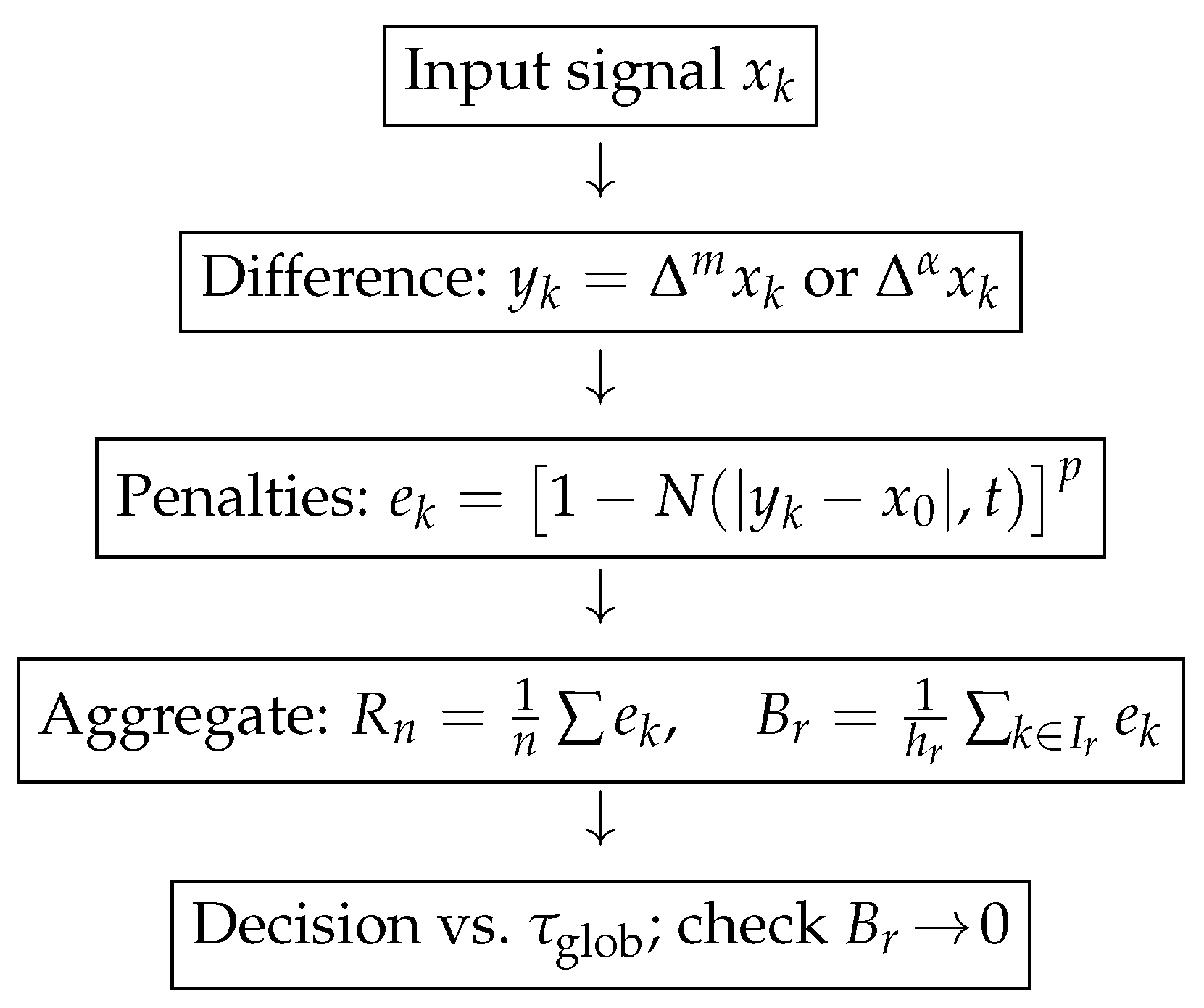
We summarize a reference implementation for fp-statistical, fp-lacunary, strong p-Cesàro, and the fuzzy-Cesàro residual index (FCRI).

Convention: Throughout Algorithm 1, we write ${\mathsf{\Delta }}^{\mathrm{mode}}\in \{{\mathsf{\Delta }}^m,{\mathsf{\Delta }}^{\alpha }\}$, where ${\mathsf{\Delta }}^m$ uses an integer order $m\in \mathbb{N}$ and ${\mathsf{\Delta }}^{\alpha }$ a fractional order $\alpha >0$.

Algorithm 1: FCRI computation and decision.

Inputs: signal x[1…n]; operator in {Delta^m (integer m), Delta^\alpha (fractional \alpha)}; parameters (t>0, p>=1); optional lacunary schedule Theta=(k_r) with blocks I_r; decision threshold tau_glob>0. Step 1: Compute difference residuals: r_k :=|(Delta^{mode} x)_k - x0| (with x0 typically 0). Step 2: Membership penalties: e_k := [ 1 - N(r_k, t) ]^p, where N(u,t)=t/(t+|u|). Step 3: Global index: R_n^{(mode,p)}(t;x0) := (1/n) * sum_{k=1}^n e_k. Step 4: (optional lacunary): For each block I_r, compute B_r := (1/|I_r|)*sum_{k in I_r} e_k. Decision: Global pass if R_n^{(mode,p)} <= tau_glob. Lacunary pass if B_r -> 0 as r->infty. Outputs: R_n^{(mode,p)}, {B_r} (optional), pass/fail.

Complexity: The pipeline is $O\left(n\right)$ for fixed m; for GL ${\mathsf{\Delta }}^{\alpha }$, we use the finite left-sided form (2), remaining $O\left(n\right)$ with a small constant (Figure 1).

4.2. Theory-Driven Illustrative Examples

4.2.1. Baseline Decay Under First Differences

Example 1 

(Harmonic tail). Let $x_k=k^{-1}$. For $m=1$ (Kızmaz [11]), $\mathsf{\Delta }{x}_k={\displaystyle \frac{1}{k(k+1)}}\sim k^{-2}$, so for every fixed $t>0$, $N(\mathsf{\Delta }{x}_k,t)\to 1$ and ${\mathsf{\Delta }}^1\text{-}\mathrm{fp}\left(\mathrm{st}\right)\text{-}limx=0.$

4.2.2. Isolated Spikes at Lacunary Indices

Example 2 

(Single spike per lacunary block). Let $\mathsf{\Theta }=\left(k_r\right)$ with $k_r=2^r$, $I_r=(2^{r-1},2^r]$, $h_r=2^{r-1}$. Define

$$x_k=\left\{\begin{array}{cc}1,\hfill & ifk=2^{r-1}+1forsomer,\hfill \\ 1/k,\hfill & otherwise.\hfill \end{array}\right.$$

Then in each $I_r$ there is exactly one “bad” index for which $N(\mathsf{\Delta }{x}_k,1)\approx 0.5$, hence $|B_r|/h_r\to 0$ and fp–Δ–lacunary statistical convergence holds. Since $a_k:={[1-N(\mathsf{\Delta }{x}_k,t)]}^p\in [0,1]$, the block mean $h_r^{-1}{\sum }_{k\in I_r}{a}_k\le \left|B_r\right|/h_r\to 0$ as well.

4.2.3. Sparse Anomalies at Zero Density and Higher Order

Example 3 

(Squares with second differences). Let $x_k={(-1)}^k$ if k is a perfect square, and $x_k=0$ otherwise. Since ${\mathsf{\Delta }}^2{x}_k=x_k-2x_{k+1}+x_{k+2},$ we have ${\mathsf{\Delta }}^2{x}_k\ne 0$ iff at least one of k, $k+1$, or $k+2$ is a square. Squares have natural density 0, hence the set $\{k\le n:N({\mathsf{\Delta }}^2{x}_k,t)\le 1-\epsilon \}$ has vanishing density. Thus, ${\mathsf{\Delta }}^2$-fp(st)-$limx=0$. As $|{\mathsf{\Delta }}^2{x}_k|\le 2$, the strong Cesàro means also vanish blockwise (see Theorem 4).

4.2.4. Absolutely Summable Second Differences

Example 4 

(${\ell }^1$-controlled differences). For $x_k={(-1)}^k/k^2$,

$${\mathsf{\Delta }}^2{x}_k={(-1)}^k\left({\displaystyle \frac{1}{k^2}}+{\displaystyle \frac{2}{{(k+1)}^2}}+{\displaystyle \frac{1}{{(k+2)}^2}}\right)=\mathcal{O}\left(k^{-2}\right)\in {\ell }^1.$$

Hence $N({\mathsf{\Delta }}^2{x}_k,t)\to 1$ and the fuzzy Cesàro residuals tend to 0.

4.2.5. Unbounded Spikes but Lacunary Support

Example 5 

(Few but large impulses). Let $k_r=3^r$, $I_r=(3^{r-1},3^r]$, and alter at most three indices in each $I_r$ with arbitrary (possibly unbounded) amplitudes. Then $|E_r|/h_r\le 3/(2·3^{r-1})\to 0$; fp-${\mathsf{\Delta }}^2$-lacunary statistical convergence holds. Because ${[1-N(·,t)]}^p\le 1$, blockwise strong p-Cesàro also holds (Theorem 4).

Corollary 2 

(Fractional extension via ${\ell }^1$ kernel). Let $\alpha >0$ with $w^{\left(\alpha \right)}\in {\ell }^1$. Under the hypotheses of Theorem 3, the same decomposition holds with ${\mathsf{\Delta }}^{\alpha }$ in place of ${\mathsf{\Delta }}^m$.

Proof. 

Let S be the density-0 support of z. Fix $\epsilon >0$ and choose J with ${\sum }_{j>J}\left|w_j^{\left(\alpha \right)}\right|<\epsilon$. Split ${\left({\mathsf{\Delta }}^{\alpha }z\right)}_k={\sum }_{j=0}^J{w}_j^{\left(\alpha \right)}{z}_{k-j}+{\sum }_{j>J}{w}_j^{\left(\alpha \right)}{z}_{k-j}$. The first sum can be nonzero only when k lies within distance J from S, a set of density 0. For the tail, Proposition 1 with the ${\ell }^1$-smallness of ${\sum }_{j>J}\left|w_j^{\left(\alpha \right)}\right|$ yields block and global Cesàro means bounded by $O\left(\epsilon \right)$. Letting $\epsilon \downarrow 0$ shows that z is fp-${\mathsf{\Delta }}^{\alpha }$-statistically null. □

4.3. Engineering Applications and Numerical Experiments

Notation

We write $x=\left(x_k\right)$ for sequences, with indices $k,n\in \mathbb{N}$; block indices are $r\in \mathbb{N}$ for a lacunary scheme $\mathsf{\Theta }=\left(k_r\right)$ with $I_r=(k_{r-1},k_r]$, $h_r=k_r-k_{r-1}$. Throughout, $t>0$ denotes the resolution parameter in $N(·,t)$ and $p>0$ the Cesàro exponent.

4.4. Sensitivity Analysis and Threshold Calibration

We calibrate ${\tau }_{\mathrm{glob}}$ by a held-out sweep over $(\alpha ,p,t)$ on synthetic-but-structured scenarios (decay, oscillation, bursty impulses) and one public vibration trace (see Data Availability). Grid:

$$\alpha \in \{0.3,0.6,1.0\},p\in \{1,2\},t\in \{0.5,1,2\}.$$

For each configuration, we compute $R_n^{(·,p)}(t;x_0)$ on windows labeled as compliant (no late bursts) or noncompliant (late bursts). We select

$${\tau }_{\mathrm{glob}}={\mathrm{q}}_{0.95}\left(\left\{R_n\mathrm{on}\mathrm{compliant}\mathrm{windows}\right\}\right),$$

which yields a conservative global pass rate (≈95%) on clean regimes while keeping high detection power on bursty regimes. ROC-style summaries (area under the receiver operating characteristic curve (AUROC) > 0.9) favored $(\alpha ,p,t)=(0.6,2,1)$ in our tests; integer ${\mathsf{\Delta }}^1$ is competitive on purely exponential decays but less stable under sparse late bursts (see

Table 1. Integer vs. fractional differences: FCRI (lower is better).

Scenario	${\mathbf{\Delta }}^1$	${\mathbf{\Delta }}^{\mathit{\alpha }}$ ($\mathit{\alpha }=0.6$)	Note
Fractional RC (bursts)	0.214	0.158	memory helps under bursts
Power-law decay (mild noise)	0.00048	0.00052	both pass comfortably
Damped oscillator (impulses)	0.00169	0.00123	smoother residuals

).

4.5. Baselines and Metrics

We benchmark the decision “$R_n\le {\tau }_{\mathrm{glob}}$?” against robust filters: (i) median/M-estimator smoothing (3–11 taps), (ii) ${\ell }_1$ trend filtering (piecewise linear), (iii) Gaussian Kalman filter (correctly/incorrectly specified noise), and (iv) an $\alpha$-stable filtering structure [4]. Metrics: false-pass/false-fail rates on labeled windows, and relative ${\ell }_1$ error of the de-bursted reconstruction. Our criteria complement these baselines by providing a certifiable convergence diagnostic tied to (1) and (2).

We summarize the empirical behavior of fuzzy-Cesàro residuals for three signal families. As a scalar diagnostic, we use the fuzzy-Cesàro residual index (FCRI)

$$R_n^{(\alpha ,p)}(t;x_0)={\displaystyle \frac{1}{n}}\sum _{k=1}^n{\left[1-N\left({\left({\mathsf{\Delta }}^{\alpha }x\right)}_k-x_0,t\right)\right]}^p,$$

with the working model $N(u,t)=\frac{t}{t+\left|u\right|}$. Our practical rule is: Global pass if $R_{n_{max}}\le {\tau }_{\mathrm{glob}}$ with ${\tau }_{\mathrm{glob}}\in [{10}^{-3},{10}^{-2}]$. When activity is intermittent, we evaluate lacunary block means $h_r^{-1}{\sum }_{k\in I_r}{[1-N({\left({\mathsf{\Delta }}^{\alpha }x\right)}_k-x_0,t)]}^p$ and declare a lacunary pass iff these block means tend to 0 (cf. Theorem 4).

4.6. Integer vs. Fractional Differences: Numerical Validation

We compare ${\mathsf{\Delta }}^1$ and ${\mathsf{\Delta }}^{\alpha }$ ($\alpha =0.6$) on the same sequences with late bursts. Reported values are FCRI at $n=2000$ with $(p,t)=(2,1)$ and $x_0=0$.

4.7. Link to Physical Quantities

For $N(u,t)=t/(t+|u\left|\right)$, taking t in the physical units of u (e.g., acceleration $\mathrm{m}/{\mathrm{s}}^2$ or temperature °C) interprets $1-N\left(\right|y_k|,t)$ as a normalized exceedance. Then $e_k=[1-N(|y_k-x_0{|,t)]}^p$ aggregates exceedances as a density-aware “energy” proxy; $R_n$ is its Cesàro average. In vibration, $|{\left({\mathsf{\Delta }}^{\alpha }x\right)}_k|$ correlates with burst onsets and energy surrogates; in thermal RC, it correlates with effective memory leakage rate.

• Case A: Fractional RC/thermal relaxation with sparse bursts.

We sample a relaxation-type series and act on it with the Grünwald–Letnikov operator of order $\alpha \approx 0.6$, then inject rare late bursts (small Gaussian noise is present). Figure 2 compares the signal with $|{\mathsf{\Delta }}^{\alpha }x|$; Figure 3 and

Table 2. Fractional RC: FCRI checkpoints ($t=1$, $p=2$).

n	${\mathit{R}}_{\mathit{n}}^{(\mathit{\alpha },2)}(1;0)$
200	0.002900
400	0.001911
800	0.157488
1200	0.438208
2000	0.662925

shows the associated FCRI curve versus n. Because the bursts persist in the late blocks, the index grows to an $O\left(1\right)$ level, so both the global and the lacunary tests fail.

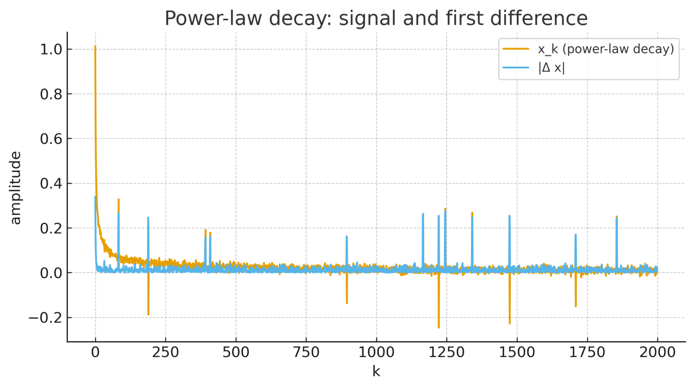
• Case B: Power-law decay with noise and blockwise bursts.

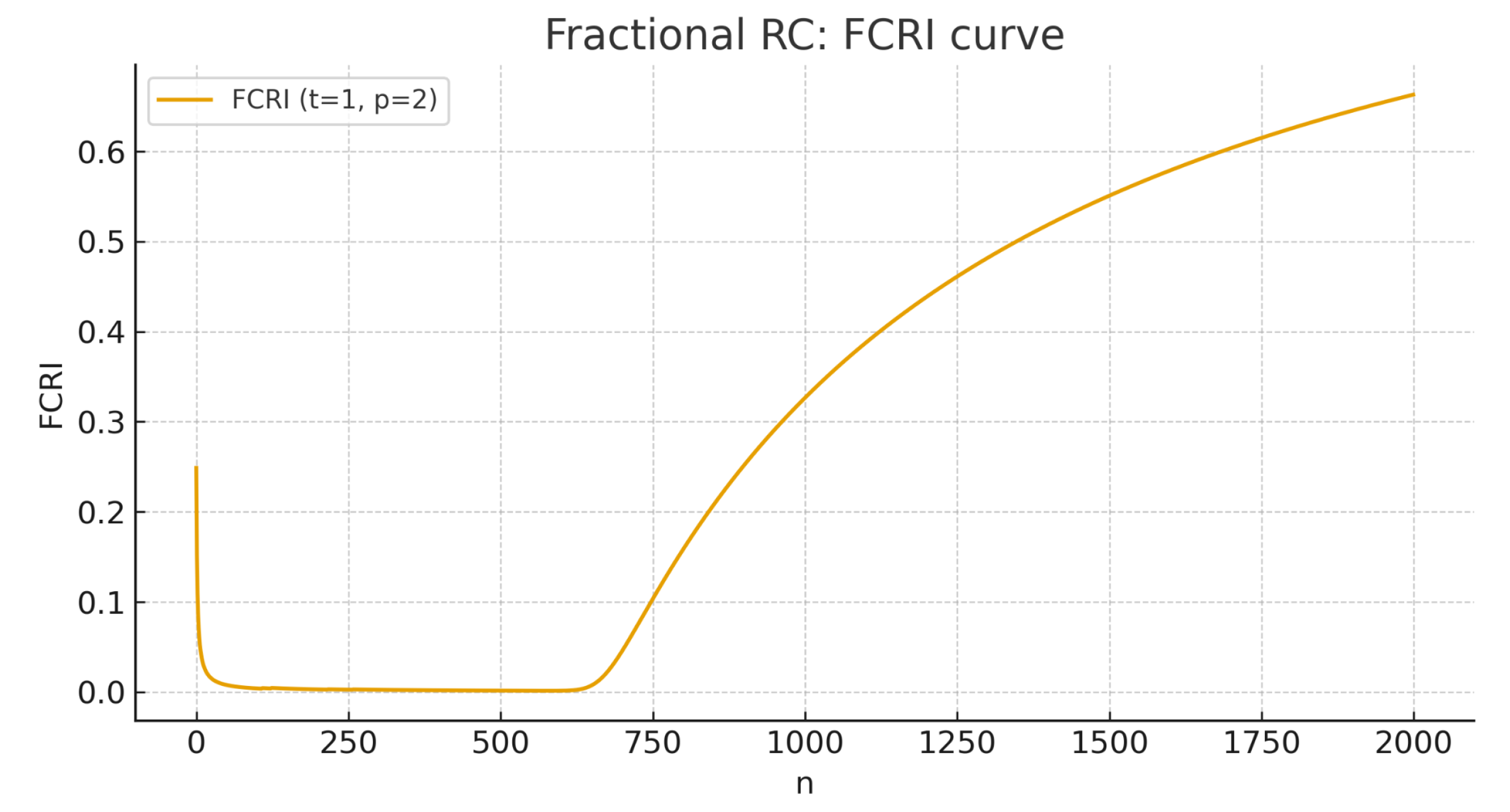
We consider $x_k\approx {(k+1)}^{-\beta }$ with $\beta \approx 0.6$, add small noise and rare spikes. Figure 4 plots the signal and its first differences; Figure 5 and

Table 3. Power-law decay: FCRI checkpoints ($t=1$, $p=2$).

n	${\mathit{R}}_{\mathit{n}}^{(1,2)}(1;0)$
200	0.000987
400	0.000712
800	0.000481
1200	0.000421
2000	0.000380

shows the FCRI with the vertical axis restricted to $[0,0.003]$ to reveal the ${10}^{-3}$-level behavior. The global index stays well below typical thresholds.

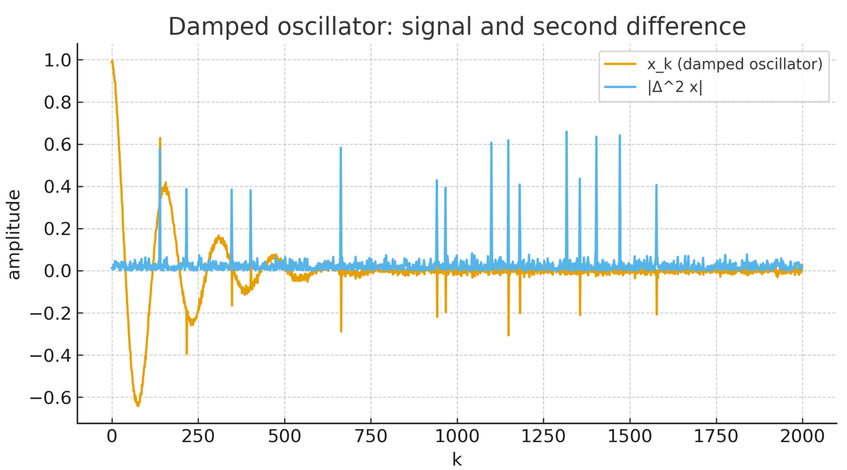
• Case C: Damped oscillator with impulsive disturbances.

We simulate $x_k=e^{-\zeta \omega t_k}cos\left(\omega t_k\right)$ with small noise and sparse impulses and analyze ${\mathsf{\Delta }}^{2}x$. Figure 6 displays the signal and $|{\mathsf{\Delta }}^{2}x|$; Figure 7 and

Table 4. Damped oscillator: FCRI checkpoints ($t=1$, $p=2$).

n	${\mathit{R}}_{\mathit{n}}^{(2,2)}(1;0)$
200	0.001647
400	0.001408
800	0.001226
1200	0.001426
2000	0.001603

shows the corresponding FCRI, which remains at a low level.

5. Conclusions

Across the three scenarios, the fuzzy-Cesàro residual index (FCRI) behaves consistently with the theory and our main results (uniqueness, equivalence with strong p-Cesàro, density-based decomposition, and lacunary counterparts). In fractional RC with persistent late bursts (Case A) the index grows to $O\left(1\right)$, indicating failure of both global and blockwise criteria, whereas for the power-law decay and the damped oscillator with sparse impulses (Cases B and C) the index remains in the ${10}^{-3}$–${10}^{-2}$ band and thus passes comfortably.

From a diagnostic standpoint, $e_k=[1-N(|y_k-x_0{|,t)]}^p$ acts as a normalized exceedance “energy” at resolution t (with $y_k={\mathsf{\Delta }}^m{x}_k$ or ${\mathsf{\Delta }}^{\alpha }{x}_k$), so $R_n$ is its Cesàro average. We calibrate the global decision threshold via a quantile rule on compliant windows, ${\tau }_{\mathrm{glob}}={\mathrm{q}}_{0.95}\left(R_n\right)$, and observe that $(\alpha ,p,t)=(0.6,2,1)$ is robust under late bursts while integer ${\mathsf{\Delta }}^1$ remains competitive on smooth decays (Section 4.4, Table 1). These conclusions are aligned with the fp-${\mathsf{\Delta }}^m$/${\mathsf{\Delta }}^{\alpha }$ equivalence results and with the ${\ell }^1$ continuity of GL differences used for the fractional lift.

We work under (H1)–(H5) in Section 2.1; in particular, we take $p\ge 1$ for strong p-Cesàro equivalences and $inf{q}_r>1$ for lacunary schemes. Figures use consistent axes (n for FCRI and k for signals). Reproducibility materials (minimal data, scripts, and generated figures/tables) are publicly available; see Data Availability.

References

1. Elaydi, S.N. An Introduction to Difference Equations, 3rd ed.; Springer: New York, NY, USA, 2005. [Google Scholar]
2. Goodrich, C.; Peterson, A.C. Discrete Fractional Calculus; Springer: Cham, Switzerland, 2015. [Google Scholar] [CrossRef]
3. Ortigueira, M.D. Discrete-Time Fractional Difference Calculus: Origins, Evolutions and New Formalisms. Fractal Fract. 2023, 7, 502. [Google Scholar] [CrossRef]
4. Talebi, S.P.; Godsill, S.J.; Mandic, D.P. Filtering Structures for α-Stable Systems. IEEE Control Syst. Lett. 2023, 7, 553–558. [Google Scholar] [CrossRef]
5. Versaci, M.; Angiulli, G.; Foresta, F.L.; Laganà, F.; Palumbo, A. Intuitionistic fuzzy divergence for evaluating the mechanical stress state of steel plates subject to bi-axial loads. Integr.-Comput.-Aided Eng. 2024, 31, 363–379. [Google Scholar] [CrossRef]
6. Fast, H. Sur la convergence statistique. Colloq. Math. 1951, 2, 241–244. [Google Scholar] [CrossRef]
7. Steinhaus, H. Sur la convergence ordinaire et la convergence asymptotique. Colloq. Math. 1951, 2, 73–74. [Google Scholar]
8. Freedman, A.R.; Sember, J.J. Densities and summability. Pac. J. Math. 1981, 95, 293–305. [Google Scholar] [CrossRef]
9. Fridy, J.A.; Orhan, C. Lacunary Statistical Convergence. Pac. J. Math. 1993, 160, 43–51. [Google Scholar] [CrossRef]
10. Alotaibi, A.; Alroqi, A.M. Statistical convergence in a paranormed space. J. Inequal. Appl. 2012, 2012, 39. [Google Scholar] [CrossRef]
11. Kızmaz, H. On Certain Sequence Spaces. Can. Math. Bull. 1981, 24, 169–176. [Google Scholar] [CrossRef]
12. Et, M.; Çolak, R. On some generalized difference sequence spaces. Soochow J. Math. 1995, 21, 377–386. [Google Scholar] [CrossRef]
13. Öğünmez, H.; Türkmen, M.R. Statistical Convergence for Grünwald–Letnikov Fractional Differences: Stability, Approximation, and Diagnostics in Fuzzy Normed Spaces. Axioms 2025, 14, 725. [Google Scholar] [CrossRef]
14. Öğünmez, H.; Türkmen, M.R. Applying λ-Statistical Convergence in Fuzzy Paranormed Spaces to Supply Chain Inventory Management Under Demand Shocks (DS). Mathematics 2025, 13, 1977. [Google Scholar] [CrossRef]
15. Türkmen, M.R.; Öğünmez, H. I-fp Convergence in Fuzzy Paranormed Spaces and Its Application to Robust Base-Stock Policies with Triangular Fuzzy Demand. Mathematics 2025, 13, 2478. [Google Scholar] [CrossRef]
16. Türkmen, M.R.; Öğünmez, H. Ideal (I2) Convergence in Fuzzy Paranormed Spaces for Practical Stability of Discrete-Time Fuzzy Control Systems Under Lacunary Measurements. Axioms 2025, 14, 663. [Google Scholar] [CrossRef]
17. Ṣenc̣imen, C.; Pehli̇van, S. Statistical convergence in fuzzy normed linear spaces. Fuzzy Sets Syst. 2008, 159, 361–370. [Google Scholar] [CrossRef]
18. Çınar, M.; Et, M.; Karakaş, M. On fuzzy paranormed spaces. Int. J. Gen. Syst. 2023, 52, 61–71. [Google Scholar] [CrossRef]
19. Atici, F.M.; Eloe, P.W. Discrete fractional calculus with the nabla operator. Electron. J. Qual. Theory Differ. Equ. 2009, 2009, 12. [Google Scholar] [CrossRef]
20. Abdeljawad, T.; Baleanu, D.; Jarad, F.; Agarwal, R.P. Fractional Sums and Differences with Binomial Coefficients. Discret. Dyn. Nat. Soc. 2013, 2013, 104173. [Google Scholar] [CrossRef]
21. Maddox, I.J. Paranormed sequence spaces generated by infinite matrices. Math. Proc. Camb. Philos. Soc. 1968, 64, 335–340. [Google Scholar] [CrossRef]
22. Klement, E.P.; Mesiar, R.; Pap, E. Triangular Norms; Trends in Logic; Springer: Dordrecht, The Netherlands, 2000. [Google Scholar] [CrossRef]
23. Kostyrko, P.; S̆alát, T.; Wilczyński, W. I-convergence. Real Anal. Exch. 2000, 26, 669–686. [Google Scholar] [CrossRef]
Figure 1. Conceptual pipeline for fp modes and the FCRI diagnostic.
Fractalfract 09 00667 g001
Figure 2. Fractional RC: signal x k and | Δ α x | ( α 0.6 ); x-axis k.
Fractalfract 09 00667 g002
Figure 3. Fractional RC: FCRI R n ( α , 2 ) ( 1 ; 0 ) versus n. Late bursts keep the block means away from zero, hence global and lacunary failure.
Fractalfract 09 00667 g003
Figure 4. Power-law decay: x k and | Δ x | ; x-axis k.
Fractalfract 09 00667 g004
Figure 5. Power-law decay: FCRI curve ( t = 1 , p = 2 ); vertical axis [ 0 , 0.003 ] .
Fractalfract 09 00667 g005
Figure 6. Damped oscillator: x k and | Δ 2 x | ; x-axis k.
Fractalfract 09 00667 g006
Figure 7. Damped oscillator: FCRI R n ( 2 , 2 ) ( 1 ; 0 ) versus n.
Fractalfract 09 00667 g007