Article

On the Qualitative Stability Analysis of Fractional-Order Corruption Dynamics via Equilibrium Points

by
Qiliang Chen
1,
Kariyanna Naveen
2,
Doddabhadrappla Gowda Prakasha
2 and
Haci Mehmet Baskonus
3,*
1
School of Economics and Finance, Chongqing University of Technology, Chongqing 400054, China
2
Department of Mathematics, Davangere University, Shivagangotri, Davangere 577007, India
3
Department of Mathematics and Science Education, Faculty of Education, Harran University, 63100 Sanliurfa, Turkey
*
Author to whom correspondence should be addressed.
Fractal Fract. 2025, 9(10), 666; https://doi.org/10.3390/fractalfract9100666
Submission received: 27 August 2025 / Revised: 11 October 2025 / Accepted: 13 October 2025 / Published: 16 October 2025

Abstract

The primary objective of this study is to provide a more precise and beneficial mathematical model for assessing corruption dynamics by utilizing non-local derivatives. This research aims to provide solutions that accurately capture the complexities and practical behaviors of corruption. To illustrate how corruption levels within a community change over time, a non-linear deterministic mathematical model has been developed. The authors present a non-integer order model that divides the population into five subgroups: susceptible, exposed, corrupted, recovered, and honest individuals. To study these corruption dynamics, we employ a new method for solving a time-fractional corruption model, which we term the q-homotopy analysis transform approach. This approach produces an effective approximation solution for the investigated equations, and data is shown as 3D plots and graphs, which give a clear physical representation. The stability and existence of the equilibrium points in the considered model are mathematically proven, and we examine the stability of the model and the equilibrium points, clarifying the conditions required for a stable solution. The resulting solutions, given in series form, show rapid convergence and accurately describe the model’s behaviour with minimal error. Furthermore, the solution’s uniqueness and convergence have been demonstrated using fixed-point theory. The proposed technique is better than a numerical approach, as it does not require much computational work, with minimal time consumed, and it removes the requirement for linearization, perturbations, and discretization. In comparison to previous approaches, the proposed technique is a competent tool for examining an analytical outcomes from the projected model, and the methodology used herein for the considered model is proved to be both efficient and reliable, indicating substantial progress in the field.

1. Introduction

Corruption comes from the Latin word “corrupts”, which means “to disrupt or harm”. Corruption is described as an illegal conduct undertaken for personal advantage via the abuse of authority by private persons [1,2]. Corruption has become a focal point in discussions of political economics and the literature regarding development. It is often characterized as dishonest or unlawful activity committed by persons or organizations in positions of power [3]. This behavior can include embezzlement, influence peddling, bribery, and other practices that may be acceptable in some nations. Corruption represents a violation of ethics, and nations allocate significant resources to counteract it. The word “anti-corruption” refers to a wide range of strategies aimed at preventing and addressing corruption [4]. Corruption is a major obstacle to attaining sustainable development goals, especially in developing nations. It is still a problem for both governments and people with low moral standards, and it has a direct correlation with poverty. Corruption is not a new phenomena; it has existed throughout history. Chanakya, an ancient Indian philosopher, felt that corruption was inherent in human nature and that resisting it was as difficult as rejecting the draw of honey. Corruption is a widespread and complicated issue that can show in a variety of ways, ranging from overt to subtle. According to the English historian Edward Gibbon, corruption is the most precise indicator of constitutional liberty. Corruption affects public trust in the sociopolitical system and promotes unfairness, dishonest behaviors, subjectivity, immorality, inefficiency, insincerity, and illegality, all of which erode society’s moral foundations and undermine public service values [5].
Corruption is a significant barrier to opportunity, as it undermines honesty and responsible investment. It increases operational costs for businesses and raises the prices of public services. Corruption knows no boundaries, affecting various institutions, including the education sector. Developing and developed countries have faced numerous negative consequences due to corruption, which has become a persistent issue. Corruption has become a frequent occurrence, characterized by bold actions and serving as a disastrous symbol of political failure that tarnishes even the most respected nations. It manifests through large-scale contract fraud at the highest levels, embezzlement, withholding of salaries, petty bribery, and money laundering schemes. Additionally, practices such as trading sex for grades, denying rightful promotions, impersonation, and cheating during examinations are prevalent and highlight the extent of corruption in various nations. Politicians in positions of power and money frequently exploit their connections to do corrupt acts. They subvert the laws they have enacted in order to pursue their own interests and selfish objectives. Law enforcement officers may harass any citizen they choose, and students may use unethical ways to pass school exams. Furthermore, few teachers are involved in exchanging sex for grades or accepting bribes to award unjustifiably high grades to college and university students. According to the Corruption Perception Index (CPI) [6], it evaluates corruption levels using various data sources, including instances of bribery, the misappropriation of public money, and the exploitation of public office for private benefit without penalties. It also assesses the government’s capability to curb corruption in the public sector, the prevalence of nepotism in civil service appointments, state control by limited entrenched interests, excessive bureaucratic hurdles, and the legal protection offered to whistleblowers reporting corruption. The CPI assesses corruption on a scale of 0–100, with 0 being a severely corrupt state and 100 representing a very clean administration. According to the statistics, Sub-Saharan Africa has the highest corruption rate in the world, with 32 points, while the European Union and Western Europe have 66 points and are free of corruption. Somalia has been classified as the nation with the highest level of corruption in the world, with a score of 12 out of 100, while Denmark has been listed as the least corrupt, with a score of 90. In 2012, it was stated that developing countries had lost over USD 4 trillion due to corruption [7]. In recent years, this threat has affected nearly every level of government, including law enforcement (police, army, immigration, and so on), education, and the courts.
Many researchers have formulated mathematical models of corruption dynamics to better understand the prevalence of corruption. Nelson and Goel [8] discovered that nations with more economic and political freedom have lower levels of corruption. Furthermore, states with a well-regulated financial sector have lower levels of corruption than those with the reverse. Dimant [9] argued, in his research, that administrative efficiency affects corruption. Another factor affecting corruption is the inadequate income of public servants, who are attempting to better their financial circumstances by accepting contributions; as a result, the socioeconomic status of the public worker influences the phenomenon of corruption. Fantaye and Birhanu [10] developed and examined an integer order corruption transmission model using optimal control strategies. The study’s findings reveal that the most effective technique for reducing the spread of corruption is prevention and punishment. Anjam et al. [11] developed a stability study of corruption dynamics utilizing fractional- order interventions.
Fractional calculus (FC) is a mathematical technique for studying derivatives and integrals of arbitrary orders. Classical calculus is a well-known subject that has received substantial attention. FC theory originated roughly 300 years ago, inspired by the work of German mathematicians L’Hospital and Leibniz. The primary benefit of non-integer order is that it offers results between intervals, making it easier to analyze the findings. Fractional order (FO) derivatives have been extensively studied for use in a variety of applications, such as engineering, physical, and control networks. The operators in FC are varied and have been utilized in a variety of approaches, such as Weyl–Riesz, Antagana–Baleanu, Grunawald–Letnikov, Riemann–Liouville, Caputo, and Caputo–Fabrizio. Each of these operators is significant and valuable in their own way. We use the Caputo derivative, which has non-local behavior and is suitable for initial solutions. It is bounded and behaves more smoothly than other fractional operators [12,13,14]. The non-integer derivative is used to model distorted dynamics caused by memory effects, which occur when earlier actions continue to influence current behavior. A few examples include prolonged public mistrust following major scandals, a pervasive culture of corruption in institutions, and the delayed consequences of anti-corruption laws. The Caputo fractional derivative’s non-locality makes it more suited than typical integer-order derivatives for expressing the long-term effects of corruption. FC is a mathematical area with applications in a variety of science and engineering disciplines. It is gaining attention in signal processing [15], electrodyna- mics [16], fluid dynamics [17], image processing [18], and many other domains [19,20,21]. Its key advantage lies in its ability to calculate derivatives up to non-integer orders, which goes beyond the limitations of traditional calculus. FC emphasizes the growing importance of mathematical applications in understanding and coping with intricate natural phenomena.
In this study, we applied a novel and effective semi-analytical approach called q-HATM, which unites the homotopy analysis technique (HAM) with Laplace transform. Chinese mathematician Liao Shijun created the HAM in 1992 [22]. This approach has been used successfully to investigate the behavior of complicated systems of equations without the requirement for linearization. This technique yields a series solution that converges swiftly inside a certain range. It might be difficult to correctly solve partial fractional differential equations and non-linear differential equations. Our technique has the distinct feature of allowing for non-linear components in partial differential equations to be discretized without the need for linearization or perturbation. This considerably lowers the computing cost of resolving non-linear complicated phenomena. The resulting solutions are more accurate than the actual answer. Singh et al. [23] introduced a novel technique termed the q-HATM approach, which combines q-HAM with the Laplace transform. This approach is extremely systematic, efficient, and precise in studying the distinct characteristics of FDE that are prominent in technology and science. This approach has been used by numerous scholars to solve various equations and models that arise in a variety of domains. Namely, Veeresha et al. [24] devised a competent strategy to explore the non-integer model of vector-borne illnesses. Naveen et al.’s [25] study on solutions of fractional order equa–width equation using novel approach. In this research, we utilized the Caputo fractional derivative in a time-dependent model. The results were obtained in series form using q-HATM, and graphs were generated to depict the behavior of the model.
The current work is innovative because we use the Caputo fractional operator to solve the time-fractional corruption dynamics using a robust semi-analytical approach called q-HATM. By combining the Laplace transform and the homotopy analysis method, this method offers a fresh way to generate series solutions with better convergence characteristics. The effectiveness of the proposed approach is shown by applying it to intricate physical models, providing a workable solution approach that may be used in a variety of scientific and technical fields. Discreteization, linearization, and perturbations are not required by the approach. Our results are in the form of quickly convergent series, and we also used 3D plots and graphs to analyze them. The technique is a potent tool for researchers exploring non-linear physical models and looking for analytical solutions for arbitrary order problems because of its versatility and accurate findings.
The proposed time-fractional corruption dynamics model has limitations. Parameter estimate might be problematic due to underreporting and measurement bias in corruption-related data, and certain values are indirectly calibrated using current research and CPI statistics. The assumptions of a homogeneous population and constant characteristics make analysis easier, but they may not capture all differences between time periods, regions, or administrative systems. Furthermore, the model’s sensitivity to beginning circumstances, particularly in FO order systems might alter results denoting the necessary for specialized sensitivity assessment. Compared to standard integer-order models, the fractional-order formulation allows for memory effects in corruption dynamics, providing a more realistic portrayal of persistence over time. The use of the q-HATM approach increases computing efficiency and accuracy. The fundamental purpose of this research is to create and evaluate a time-fractional non-linear deterministic mathematical model of corruption dynamics using the q-HATM and the Caputo fractional derivative. The goal is to evaluate equilibrium point stability, capture the persistence and memory effects involved in the corruption process, and produce exact semi-analytical conclusions that correctly represent actual corruption dynamics.
The layout of this document is as follows: The definitions and characteristics of the LT and FC are examined in Section 2. The construction of a mathematical model is shown in Section 3. While Section 5 shows the existence and stability of the equilibrium points, Section 4 presents the q-HATM technique, which uses the Caputo operator to examine the results of the fractional corruption model. In Section 6, solutions and graphical representations of the model under investigation are provided using the proposed approach. Our results and graphs are discussed in Section 7, and our conclusions are compiled in Section 8.

2. Preliminaries

Some important ideas pertaining to LT and FC will be reviewed.
Definition 1. 
The Riemann–Liouville [12] (RL) arbitrary integral in the sense is denoted by J ε τ f ( ε ) . For a function [13] f ε C τ τ 1 ,
J ε τ f ( ε ) = 1 Γ τ 0 ε τ v τ 1 f ( v ) d v , τ , ε > 0 , J ε τ f ( ε ) = f ( ε ) , τ = 0 , ε > 0 .
where Γ ( τ ) denotes the Gamma function and C τ shows continuous function domain.
Definition 2. 
In [14] the Caputo sense, the non-integer derivative of function f C 1 η is defined as
D ε τ f ( ε ) = d n f ( ε ) d ε n , τ = n N , 1 Γ ( n τ ) 0 ε ( τ v ) n τ 1 f ( n ) ( v ) d v , n 1 < τ < n , n N .
The Caputo fractional derivative has the following linear property:
D ε τ ( λ x ( ε ) + μ y ( ε ) ) = λ D ε τ x ( ε ) + μ D ε τ y ( ε ) ,
the set of natural numbers is represented by N , whereas certain constants are μ and λ.
Definition 3. 
For the [13] function D ε τ f ( ε ) , a Caputo [14] fractional derivative’s L T is stated as follows
L D ε τ f ( ε ) = s τ F s η 1 r = 0 s τ r 1 f ( r ) 0 + , n 1 < τ n ,
where F ( s ) symbolize the LT of f ( ε ) .
Definition 4. 
The Mittag–Leffler [14] function E ε z is a generalization of the exponential function and plays a key role in solutions of fractional-order differential equations. While the exponential function models processes with a constant rate of change, the Mittag–Leffler function allows for rates that change over time, making it suitable for systems.
E ε z = r = 0 z τ Γ ε τ + 1 , ε > 0 , z C .

3. Model Formulation

This section describes how to build the proposed model. For each time ξ 0 , the population under study, say N ( ξ ) , is separated into five categories: S ( ξ ) denotes susceptible individuals, E ( ξ ) denotes exposed individuals, C ( ξ ) denotes corrupted individuals, R ( ξ ) is recovered individuals, and H ( ξ ) represents honest individuals. Additionally, the model formulation has certain parameters: μ represents the human population’s overall mortality rate; ψ is the percentage of persons who join the honest population from the susceptible population; ε is the rate at which recovered individuals become honest; the chance of corruption transmission per contact is β , as vulnerable people will engage with exposed persons at a rate; δ denotes the rate at which persons exposed to corruption get corrupted; ρ and π are the recruitment rate of susceptible humans; θ denotes the fraction of people who transition from the recovered compartment to the honest sub-population; and α is the percentage of individuals from the exposed compartment who join the corrupted [11] sub-population. As a result, the whole population at any given moment ξ is as follows:
N ( χ ) = S ( χ ) + E ( χ ) + C ( χ ) + R ( χ ) + H ( χ ) .
As a result, a set of non-linear differential equations will regulate the fundamental corruption dynamic model, where
d S d χ = Π + ( 1 θ ) R ρ β SC ( ψ + μ ) S , d E d χ = ρ β SC ( δ + μ ) E , d C d χ = α δ E ( σ + μ ) C , d R d χ = σ C + ( 1 α ) δ E ( + μ ) R , d H d χ = ψ S + θ R μ H ,
along with the initial settings:
S ( 0 ) = S 0 0 , E ( 0 ) = E 0 0 , C ( 0 ) = C 0 0 , R ( 0 ) = R 0 0 , H ( 0 ) = H 0 0 .
In our study of corruption dynamics, we utilize the Caputo derivative with non-integer order rather than traditional integer-order time derivative. This non-integer approach allows us to understand the effects of memory and offers deeper insights into corruption dynamics. We also provide several crucial concepts and conclusions related to fractional calculus that are necessary for this approach. A fractional differential equation is an extension of an ordinary differentiation equation since it allows for a large degree of freedom in determining the order of the derivative. It can be applied in the linear as well as the non-linear differential equation in a straightforward manner as an ordinary differentiation equation. This model Equation (5) is transformed in the form of fractional differential equations as follows [11]:
d τ S d χ τ = Π + ( 1 θ ) R ρ β SC ( ψ + μ ) S , d τ E d χ τ = ρ β SC ( δ + μ ) E , d τ C d χ τ = α δ E ( σ + μ ) C , d α R d χ τ = σ C + ( 1 α ) δ E ( + μ ) R , d τ H d χ τ = ψ S + θ R μ H .
along with the starting conditions:
S ( 0 ) = S 0 0 , E ( 0 ) = E 0 0 , C ( 0 ) = C 0 0 , R ( 0 ) = R 0 0 , H ( 0 ) = H 0 0 .

4. Fundamental Procedure for Suggested Method

The procedures for applying the q-HATM to solve the non-linear fractional PDE are given in this section [23]. Let us look at a general version of the non-linear, [24] non-homogeneous PDE of non-integer order, which is provided by
D ε τ ϑ ( ζ , χ ) + ϑ ( ζ , χ ) + N ϑ ( ζ , χ ) = f ( ζ , χ ) , 0 < τ 1 ,
where D ε τ ϑ ( ζ , χ ) represents the Caputo non-integer derivative of the function ϑ ( ζ , χ ) , f ( ζ , χ ) is the source term, and N denotes non-linear and indicates the linear differential operator, which is bounded in χ and ζ . By employing LT for Equation (7), we achieve
L τ [ ϑ ( ζ , χ ) ] k = 1 r 1 s τ k 1 ϑ k ( ζ , 0 ) + L [ N ϑ ( ζ , χ ) ] + L [ ϑ ( ζ , χ ) ] = L [ f ( ζ , χ ) ] .
On dissecting Equation (8), we obtain
L ϑ ( ζ , χ ) 1 s τ k = 1 r 1 s τ k 1 ϑ k ( ζ , 0 ) + 1 s τ L [ N ϑ ( ζ , χ ) ] + L [ ϑ ( ζ , χ ) ] L [ f ( ζ , χ ) ] = 0 .
N is the non-linear operator and it is demonstrated as
N [ φ ( ζ , χ ; q ) ] = L [ φ ( ζ , χ ; q ) ] 1 s τ k = 1 r 1 s τ k 1 φ k ( ζ , χ ; q ) ( 0 + ) 1 s τ L [ φ ( ζ , χ ; q ) ] + L [ N φ ( ζ , χ ; q ) ] L [ f ( ζ , χ ) ] ,
then, H ( ζ , χ ) is the deformation equation,
L φ ( ζ , χ ; q ) ϑ 0 ( ζ , χ ) 1 n q = q N H ( ζ , χ ) φ ( ζ , χ ; q ) ,
with φ ( ζ , χ ; q ) representing a real unknown function and ϑ 0 ( ζ , χ ) representing the initial solution, and q represents the embedding parameter, which is within the range [ 0 , 1 r ] . The auxiliary parameter is 0 , and the LT is represented by L . The terms that follow apply to both q = 0 and q = 1 r , respectively.
φ ζ , χ ; 1 r = ϑ ( ζ , χ ) , φ ( ζ , χ ; 0 ) = ϑ 0 ( ζ , χ ) .
By varying q between 0 and 1 r , the outcome φ ( ζ , χ ; q ) converges from ϑ 0 ( ζ , χ ) to the solution ϑ ( ζ , χ ) . A series form of the function, φ ( ζ , χ ; q ) , is then expanded using the Taylor theorem for all of q.
φ ( ζ , χ ; q ) = ϑ 0 ( ζ , χ ) + m = 1 ϑ r ( ζ , χ ) q r ,
where
ϑ r ( ζ , χ ) = 1 r ! r φ ( ζ , χ ; q ) q r | q = 0 .
Let r be the auxiliary linear operator and represent a specific choice of auxiliary parameter. The series Equation (13) converges at q = 1 r for the beginning estimation ϑ 0 ( ζ , ε ) and H ( ζ , ε ) appropriately, which yields the results to the basic non-linear Equation (7), of the type
ϑ ( ζ , χ ) = ϑ 0 ( ζ , χ ) + r = 1 ϑ r ( ζ , χ ) 1 r r .
To obtain the order r deformation equation, first differentiate the deformation equation Equation (11) up to r-times with reference to q, then divide by m ! , and lastly consider q = 0
L ϑ m ( ζ , χ ) K r ϑ r 1 ( ζ , χ ) = H ( ζ , χ ) r ( ϑ r 1 ) ,
where
K r = 0 r 1 , r o t h e r w i s e ,
and
r ( ϑ r 1 ) = 1 r 1 r 1 N φ ( ζ , χ ; q ) q m 1 | q = 0 .
The vectors are regarded as
ϑ r = ϑ 0 ( ζ , χ ) , ϑ 1 ( ζ , χ ) ϑ r ( ζ , χ ) .
The recursive equation is represented as Equation (16) after the Laplace inverse transform of the deformation equation is performed.
ϑ r ( ζ , χ ) = K r ϑ r 1 ( ζ , χ ) + L 1 [ r ( ϑ r 1 ) ] .
There are iterative terms for ϑ m ( χ ) that can be obtained after solving Equation (20). The q-HATM result is described here in series form.
ϑ ( ζ , χ ) = r = 0 ϑ r ( ζ , χ ) .

5. Existence of the Equilibrium Points and Their Stability

The rate at which a system changes over time must be zero in order for it to be in equilibrium. The Equation (6) is solved by setting the right-hand side to zero. Consequently, we are able to determine the model’s equilibrium points.
d S d χ = d E d χ = d C d χ = d R d χ = d H d χ = 0 . s
Therefore,
Π + ( 1 θ ) R ρ β S C ( κ + μ ) S = 0 , ρ β S C ( δ + μ ) E = 0 , α δ E ( σ + μ ) C = 0 , σ C + ( 1 α ) δ E ( + μ ) R = 0 , κ S + θ R μ H = 0 .
We solve the aforementioned set of equations to determine the equilibrium points,
E 1 = π ( κ + μ ) , 0 , 0 , 0 , ( κ π ) ( κ μ + μ 2 ) ,
E 2 = ( δ + μ ) ( μ + σ ) α β δ ρ , ( ( ϵ + μ ) ( μ + σ ) ( μ ( κ + μ ) ( μ + σ ) + δ ( μ 2 + μ σ + κ ( μ + σ ) α β ρ π ) ) ) ( α β δ ρ ] ( α δ ϵ ( 1 + θ ) μ ( μ ( ϵ + μ ) + δ ( ϵ θ + μ ) ) ( μ + σ ) ) ) , ( ( ϵ + μ ) ( μ ( κ + μ ) ( μ + σ ) + δ ( μ 2 + μ σ + κ ( μ + σ ) α β ρ π ) ) ) ( β ρ ( α δ ϵ ( 1 + θ ) μ ] ( μ ( ϵ + μ ) + δ ( ϵ θ + μ ) ) ( μ + σ ) ) ) , ( 1 + α ) μ σ ) ( μ ( κ + μ ) ( μ + σ ) + δ ( μ 2 + μ σ + κ ( μ + σ ) α β ρ π ) ( ( α β ρ ( α δ ϵ ( 1 + θ ) μ ( μ ( ϵ + μ ) + δ ( ϵ θ + μ ) ) ( μ + σ ) ) ) , ( δ + μ ) ( κ μ ( ϵ + μ ) δ κ ( ϵ θ + μ ) + δ 2 ϵ ( κ + μ ) ) ( μ + σ ) 2 + α 2 β δ 3 ϵ μ ρ π α δ ϵ ( μ + σ ) ( ( ( 1 + θ ) κ μ 2 ) + δ ( μ 3 + κ μ ( 1 θ + μ ) ) + δ 2 ( κ μ + μ 2 + β ρ π ) ) ( α β δ μ ρ ( α δ ϵ ( 1 + θ ) μ ( μ ( ϵ + μ ) + δ ( ϵ θ + μ ) ) ( μ + σ ) ) ) , = ( 111.111 , 1056.08 , 2437.1 , 470.551 , 2266.99 ) . For the model under consideration, the Jacobian matrix J is as follows
J = ρ β C ( κ + μ ) 0 ρ β S ( 1 θ ) ε 0 ρ β C ( δ + μ ) ρ β S 0 0 0 α δ ( σ + μ ) 0 0 0 ( 1 α ) δ σ ( ε + μ ) 0 κ 0 0 θ ε μ .
The following is the Jacobian matrix at the equilibrium point E 1 :
J E 1 = 0.046 0 1.55661 0.315 0 0 0.216 1.55661 0 0 0 0.06 0.026 0 0 0 0.14 0.01 0.366 0 0.03 0 0 0.035 0.016 .
The eigenvalues associated with the matrix J E 1 are
ω 11 = 0 . 441034 , ω 12 = 0 . 366 , ω 13 = 0 . 199034 , ω 14 = 0 . 046 , ω 15 = 0 . 016 .
At the equilibrium point E 2 , the Jacobian matrix is
J E 2 = 2.09901 0 0.0936 0.315 0 2.05301 0.216 0.0936 0 0 0 0.06 0.026 0 0 0.03 0 0 0.035 0.016 .
The eigenvalues corresponding to the above matrix are
ω 21 = 2 . 07352 , ω 22 = 0 . 541314 , ω 23 = 0 . 0745056 , ω 24 = 0 . 0176722 , ω 25 = 0 . 016 .
To investigate the stability of the system, the eigenvalues of the matrix at two equilibrium point are computed. The equilibrium point E 1 was found to be unstable, while the second equilibrium point E 2 became stable as all eigenvalues were negative. Depending on starting conditions and parameter settings, slight departures from these states may result in trajectories that diverge toward larger or lower corruption prevalence. This instability highlights how hard it is to keep a state free of corruption and how ongoing, successful anti-corruption efforts are essential to guiding the system in the direction of desired results. Consequently, we analyze the eigenvalues of the Jacobian matrix generated by linearizing the system around each equilibrium point to ascertain if these points are stable. We may categorize the equilibrium point’s stability condition using the eigenvalues nature, which offers important information about the system’s long-term behavior.
Theorem 1 
(Convergence theorem ). By Banach’s fixed-point theorem, the q-HATM iterative scheme converges under contraction conditions, ensuring that the obtained semi-analytical solutions are unique, stable, and reliable.
Let K be a [26] Banach Space and F : M M be a non-linear mapping, then assume that
F ( u ) F ( w ) μ i u w , u , w M .
As a result, their existing fixed point converges to a solitary point is H, and
w m w n μ i p 1 μ i w 1 w 0 , i = 1 , 2 , 3
Proof. 
The Banach space ( C [ J ] , · ) with norm specified as g ( χ ) = max ϑ J g ( χ ) function on J.
Currently, we confirm S m , { E m } , C m , { R m } , { H m } the sequence is Cauchy in ( C [ J ] , · ) . For S, take into consideration
S m S n = max χ j S | S m S n | ,
S m S n = max χ J S m S n , = max χ J ( S m 1 S n 1 ) ( K m + ) L 1 [ 1 s τ L [ π + ( 1 θ ) ε ( R m 1 R p 1 ) ρ β ( S m 1 C m 1 S n 1 C n 1 ) ( ψ + μ ) ( S m 1 S n 1 ) ] , max χ J | ( S m 1 S n 1 ) ( K m + ) | | 0 χ π + ( 1 θ ) ε ( R m 1 S n 1 ) ρ β ( S m 1 C m 1 S n 1 C n 1 ) ( ψ + μ ) ( S m 1 S n 1 ) ( χ v ) α Γ ( α + 1 ) d v | .
According to the [27] theorem of convolution for LT. We follow
S m S n | K m + S m 1 S n 1 | π + ( 1 θ ) ε δ 4 ρ β ( δ 1 + δ 3 ) ( ψ + μ ) δ 1 ( χ v ) α Γ ( 1 + α ) | S m 1 S n 1 | .
where
δ 1 = S m 1 S n 1 , δ 2 = E m 1 E n 1 , δ 3 = C m 1 C n 1 , δ 4 = R m 1 R n 1 , δ 5 = H m 1 H n 1 .
Using the mean value theorem, the aforementioned inequality is diminished [28]. The resulting equation is showing in Equation (29):
S m S n μ 1 S m 1 S n 1 .
Take m = n + 1 ; it yields
S n + 1 S n μ 1 S n S n 1 μ 1 2 S n 1 S n 2 μ 1 n S 1 S 0 .
By employing the triangular inequality,
S n S n 1 S n + 1 S n + S n + 2 S n + 1 + S n S n 1 μ 1 n + μ 1 n + μ 1 n 2 + μ 1 m 1 S 1 S 0 μ 1 n 1 μ 1 m n 1 1 μ 1 S 1 S 0 .
As 0 μ 1 , so 1 μ m n 1 < 1 ; then we have
S n + 1 S n μ 1 n 1 μ 1 S 1 S 0 .
S n + 1 S n 0 shows that S n is a Cauchy sequence. However, S 1 S 0 < as m .
Similarly, we have
E n + 1 E n μ 1 n 1 μ 1 E 1 E 0 ,
C n + 1 C n μ 1 p 1 μ 1 C 1 C 0 ,
R n + 1 R n μ 1 p 1 μ 1 R 1 R 0 ,
H n + 1 H n μ 1 p 1 μ 1 H 1 H 0 .
Theorem 2 
(Uniqueness theorem). The outcome of projected non-integer [26] differential equation through q-HATM is unique, whenever 0 < μ i < 1 , i = 1 , 2 , 3 , 4 .
Proof. 
The given equation yields the following results:
In general,
w ( ζ , χ ) = m = 0 w m ( ζ , χ ) ,
suppose S , S * be two different values ∋ S S * max χ j S S * , for i = 1
S m ( ζ , χ ) | K m + h S S * L 1 1 s τ π + ( 1 + θ ) ε R ρ β SC + ρ R ( ψ + μ ) S | , | K m + h S S * | h | 0 t π + ( 1 + θ ) ε ( R R * ) ρ β ( S S * ) ( C C * ) + ρ R ( ψ + μ ) ( S S * ) | , | K m + h S S * | h | 0 t π + ( 1 + θ ) ε ( R m 1 R p 1 * ) ρ β ( S m 1 S m 1 * ) ( C p 1 C p 1 * ) + ρ R ( ψ + μ ) ( S m 1 S p 1 * ) | ,
(By convolution theorem)
| K m + h S S * | | 0 t π + ( 1 + θ ) ( R R * ) ρ β ( SC S * C * ) ( ψ + μ ) ( S S * ) χ v α Γ ( 1 + α ) S * d v | ,
The above inequality related to
| S S * | μ S | S S * | ,
where
μ s = K m + h S S * 0 t π + ( 1 θ ) δ 4 ρ β ( δ 1 + δ 3 ) ( ψ + μ ) δ 1 t v α Γ 1 + α S S * d v ,
where δ 1 = S m 1 S n 1 , δ 2 = E m 1 E n 1 , δ 3 = C m 1 C n 1 , δ 4 = R m 1 R n 1 , δ 5 = H m 1 H n 1 ,
We get
1 μ 1 | S S * | 0 ,
| S S * | = 0 , 0 < μ < 1 ,
S = S * .
Similarly,
E = E * ,
C = C * ,
R = R * ,
H = H * .

6. Solution of the Projected Model Using q-HATM

Application 1.
Contemplating the following time-fractional [11] corruption model, we have
d τ S d χ τ = Π + ( 1 θ ) R ρ β SC ( ψ + μ ) S , d τ E d χ τ = ρ β SC ( δ + μ ) E , d τ C d χ τ = α δ E ( σ + μ ) C , d τ R d χ τ = σ C + ( 1 α ) δ E ( + μ ) R , d τ H d χ τ = ψ S + θ R μ H ,
subjected to starting condition
S ( 0 ) = 10 , 000 , E ( 0 ) = 0 , C ( 0 ) = 100 , R ( 0 ) = 0 , H ( 0 ) = 100 .
By applying the LT to Equation (29), and taking into consideration the starting solution provided in Equation (30), we obtain
L S ( ζ , χ ) 1 S ( S 0 ) 1 S τ L π + ( 1 θ ) ε R ρ β SC ( ψ + μ ) S = 0 , L E ( ζ , χ ) 1 S ( E 0 ) 1 S τ L ρ β SC ( δ + μ ) E = 0 , L C ( ζ , χ ) 1 S ( C 0 ) 1 S τ L α δ E ( σ + μ ) C = 0 , L R ( ζ , χ ) 1 S ( R 0 ) 1 S τ L σ C + ( 1 σ ) δ E ( ε + μ ) R = 0 , L H ( ζ , χ ) 1 S ( H 0 ) 1 S τ L ψ S + θ ε R μ H = 0 .
We can use the suggested technique by describing N as the non-linear operator represented by the following:
N 1 [ φ 1 ( ζ , χ ; q ) , φ 2 ( ζ , χ ; q ) , φ 3 ( ζ , χ ; q ) φ 4 ( ζ , χ ; q ) , φ 5 ( ζ , χ ; q ) ] = L [ φ 1 ( ζ , χ ; q ) ] 1 S ( S 0 ) 1 S τ L π + ( 1 θ ) ε φ 4 ( ζ , χ ; q ) ρ β φ 1 ( ζ , χ ; q ) φ 3 ( ζ , χ ; q ) ( ψ + μ ) φ 1 ( ζ , χ ; q ) , N 2 [ φ 1 ( ζ , χ ; q ) , φ 2 ( ζ , χ ; q ) , φ 3 ( ζ , χ ; q ) φ 4 ( ζ , χ ; q ) , φ 5 ( ζ , χ ; q ) ] = L [ φ 2 ( ζ , χ ; q ) ] 1 S ( E 0 ) 1 S τ L ρ β φ 1 ( ζ , χ ; q ) φ 3 ( ζ , χ ; q ) ( δ + μ ) φ 2 ( ζ , χ ; q ) , N 3 [ φ 1 ( ζ , χ ; q ) , φ 2 ( ζ , χ ; q ) , φ 3 ( ζ , χ ; q ) φ 4 ( ζ , χ ; q ) , φ 5 ( ζ , χ ; q ) ] = L [ φ 3 ( ζ , χ ; q ) ] 1 S ( C 0 ) 1 S τ L α δ φ 1 ( ζ , χ ; q ) φ 3 ( ζ , χ ; q ) ρ φ 2 ( ζ , χ ; q ) ( σ + μ ) φ 3 ( ζ , χ ; q ) , N 4 [ φ 1 ( ζ , χ ; q ) , φ 2 ( ζ , χ ; q ) , φ 3 ( ζ , χ ; q ) φ 4 ( ζ , χ ; q ) , φ 5 ( ζ , χ ; q ) ] = L [ φ 4 ( ζ , χ ; q ) ] 1 S ( R 0 ) 1 S τ L σ φ 3 ( ζ , χ ; q ) + ( 1 α ) δ φ 2 ( ζ , χ ; q ) ( ε + μ ) φ 4 ( ζ , χ ; q ) . N 5 [ φ 1 ( ζ , χ ; q ) , φ 2 ( ζ , χ ; q ) , φ 3 ( ζ , χ ; q ) φ 4 ( ζ , χ ; q ) , φ 5 ( ζ , χ ; q ) ] = L [ φ 4 ( ζ , χ ; q ) ] 1 S ( H 0 ) 1 S τ L ψ φ 1 ( ζ , χ ; q ) + θ ε φ 4 ( ζ , χ ; q ) μ φ 5 ( ζ , χ ; q ) .
Using the suggested approach, the deformation equation is defined as
L [ S r ( ζ , χ ) k r S r 1 ( ζ , χ ) ] = L 1 { 1 , r [ S r 1 , E r 1 , C r 1 , R r 1 , H r 1 ] } , L [ E r ( ζ , χ ) k r E r 1 ( ζ , χ ) ] = L 1 { 2 , r [ S r 1 , E r 1 , C r 1 , R r 1 , H r 1 ] } , L [ C r ( ζ , χ ) k r C r 1 ( ζ , χ ) ] = L 1 { 3 , r [ S r 1 , E r 1 , C r 1 , R r 1 , H r 1 ] } , L [ R r ( ζ , χ ) k r R r 1 ( ζ , χ ) ] = L 1 { 4 , r [ S r 1 , E r 1 , C r 1 , R r 1 , H r 1 ] } , L [ H r ( ζ , χ ) k r H r 1 ( ζ , χ ) ] = L 1 { 5 , r [ S r 1 , E r 1 , C r 1 , R r 1 , H r 1 ] } ,
where
1 , r S r 1 , E r 1 , C r 1 , R r 1 , H r 1 = L [ S r 1 ( ζ , χ ) ] 1 k r n 1 S S 0 1 S τ L π + ( 1 θ ) ε R r 1 ρ β i = 0 r 1 S i C r 1 i ( ψ + μ ) E r 1 , 2 , r S r 1 , E r 1 , C r 1 , R r 1 , H r 1 = L [ E r 1 ( ζ , χ ) ] 1 k r n 1 S E 0 1 S τ L ρ β i = 0 r 1 S i C r 1 i ( ψ + μ ) E r 1 , 3 , r S r 1 , E r 1 , C r 1 , R r 1 , H r 1 = L [ C r 1 ( ζ , χ ) ] 1 k r n 1 S C 0 1 S τ L α δ E r 1 ( σ + μ ) C r 1 , 4 , r S r 1 , E r 1 , C r 1 , R r 1 , H r 1 = L [ R r 1 ( ζ , χ ) ] 1 k r n 1 S R 0 1 S τ L σ C r 1 + ( 1 α ) δ E r 1 ( ε + μ ) R r 1 , 5 , r S r 1 , E r 1 , C r 1 , R r 1 , H r 1 = L [ H r 1 ( ζ , χ ) ] 1 k r n 1 S H 0 1 S τ L ψ S r 1 + θ ε R r 1 μ H m 1 .
Employing inverse LT Equation (33), we obtain
S r ζ , χ = k r S r 1 ( ζ , χ ) + L 1 1 , r S r 1 , E r 1 , C r 1 , R r 1 , H r 1 , E r ζ , χ = k r E r 1 ( ζ , χ ) + L 1 2 , r S r 1 , E r 1 , C r 1 , R r 1 , H r 1 , C r ζ , χ = k r C r 1 ( ζ , χ ) + L 1 3 , r S m 1 , E r 1 , C r 1 , R r 1 , H r 1 , R r ζ , χ = k r R r 1 ( ζ , χ ) + L 1 4 , r S r 1 , E r 1 , C r 1 , R r 1 , H r 1 , H m ζ , χ = k r H r 1 ( ζ , χ ) + L 1 5 , r S r 1 , E r 1 , C r 1 , R r 1 , H r 1 .
To obtain a solution for Equation (33), follow the steps outlined below:
S 0 = 10 , 000 ,
E 0 = 0 ,
C 0 = 100 ,
R 0 = 0 ,
H 0 = 100 ,
S 1 ζ , χ = 1217.4 χ τ Γ τ + 1 ,
E 1 ζ , χ = 842.4 χ τ Γ τ + 1 ,
C 1 ζ , χ = 2.6 χ τ Γ τ + 1 ,
R 1 ζ , χ = 1 χ τ Γ τ + 1 ,
H 1 ζ , χ = 298.4 χ τ Γ τ + 1 .
. . .
We can achieve additional iterative terms in this way. The final essential series solution of Equation (29) utilizing q-HATM is represented as follows:
S ζ , χ = S 0 ζ , χ + r = 1 S r ( ζ , χ ) 1 n r , E ζ , χ = E 0 ζ , χ + r = 1 E r ( ζ , χ ) 1 n r , C ζ , χ = C 0 ζ , χ + r = 1 C r ( ζ , χ ) 1 n r , R ζ , χ = R 0 ζ , χ + r = 1 R r ( ζ , χ ) 1 n r , H ζ , χ = H 0 ζ , χ + r = 1 H r ( ζ , χ ) 1 n r .

7. Results and Discussion

In this research, we have successfully utilized an efficient results procedure called q-HATM to examine the outcomes for the time-fractional corruption model. This study presents a non-linear deterministic mathematical model that captures the dynamics of corruption levels within a population. The author has developed a fractional order model to analyze these dynamics. This model divides the overall individuals into five categories: susceptible, exposed, corrupted, recovered (against corruption), and honest individuals. The suggested model consists of a system of equations that are analyzed, and the Caputo operator is utilized to investigate the time-fractional derivative. As non-integer order systems are sensitive to starting solutions, the key parameters were chosen from published corruption dynamics research and calibrated regarding qualitative trends from the Corruption Perception Index (CPI) and related socio-economic indicators. This proper choice ensures predictive reliability and offers a stable representation of corruption dynamics in spite of the system’s inherent sensitivity. The results are achieved utilizing the semi-analytical method known as q-HATM. In order to solve the system of equations, we assessed the starting setting’s values, including S = 10 , 000 , E = 0 , C = 100 , R = 0 , and H = 100 . The time-fractional mathematical corruption model’s simplified form with the relevant parameters is provided as follows [11]:
Parameter ρ β δ ε π ψ μ α θ
Value 0.036 0.0234 0.2 0.35 85 0.03 0.0160 0.3 0.1
These are chosen because they are qualitatively consistent with observed corruption prevalence rates and transition behaviors from empirical studies [6,7,8,9], as well as because they are reported in previous corruption dynamics and the related socio-epidemiological modeling literature [10,11]. Since fractional-order systems are known to be sensitive to initial conditions, we examined the robustness of the model under the chosen parameter set. The parameters were selected based on published corruption dynamics studies and calibrated against qualitative trends reported in the Corruption Perception Index (CPI) and related socio-economic indicators. Where direct measurements were not available, values were chosen to remain consistent with realistic prevalence and transition behaviors. Sensitivity to the fractional order τ was also tested, and the results show consistent qualitative patterns across different values. This confirms that the adopted parameter set enhances the predictive reliability of the model and provides a stable representation of corruption dynamics despite the system’s inherent sensitivity. The model assumes a “homogeneous population”, where all individuals share similar characteristics regarding their involvement in or resistance to corruption, and “constant parameters over time”, implying fixed rates of spread, prevention, and enforcement. These simplifications, common in initial corruption modeling, enable analytical tractability, but may not capture temporal or subgroup variations present in reality. Future extensions could incorporate heterogeneity, time-varying parameters, and stochastic influences to enhance real-world applicability.
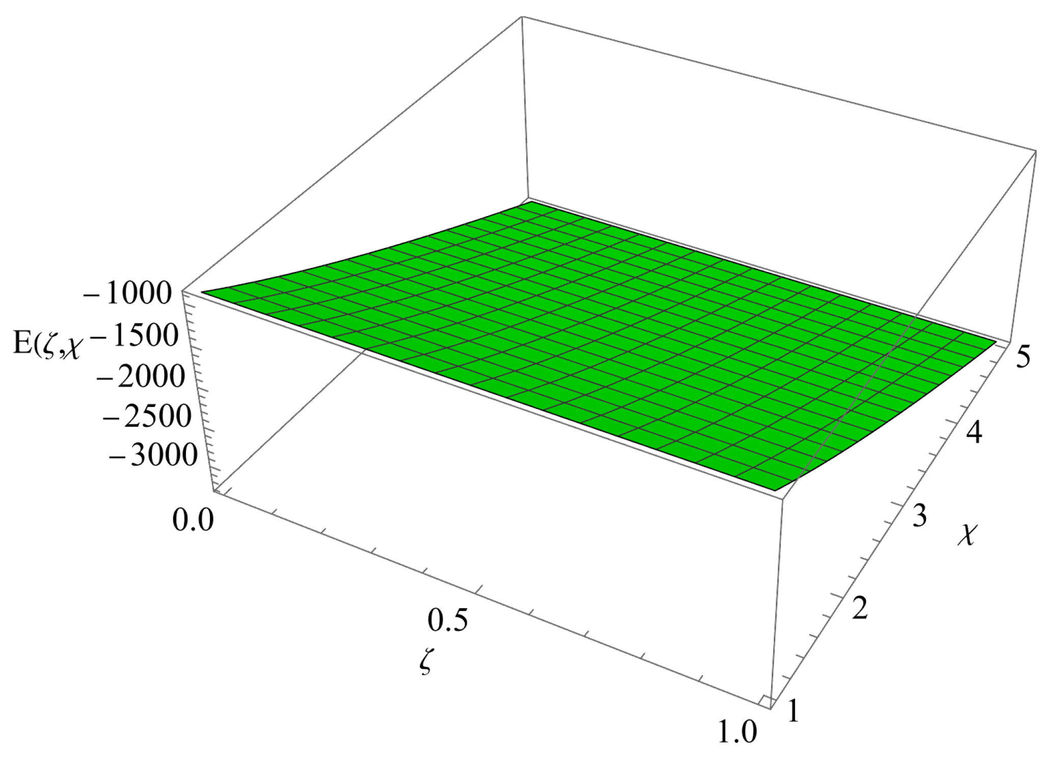
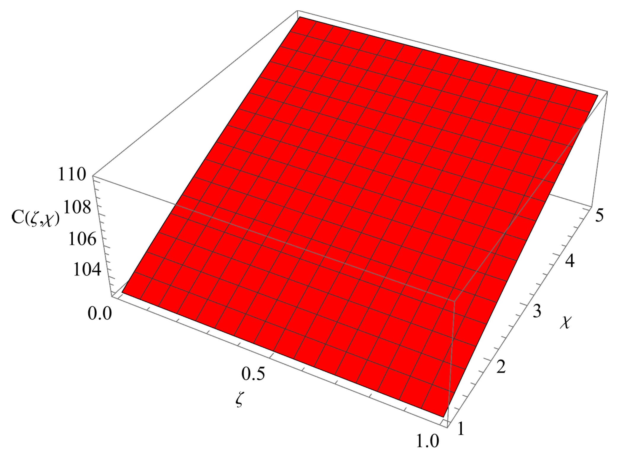
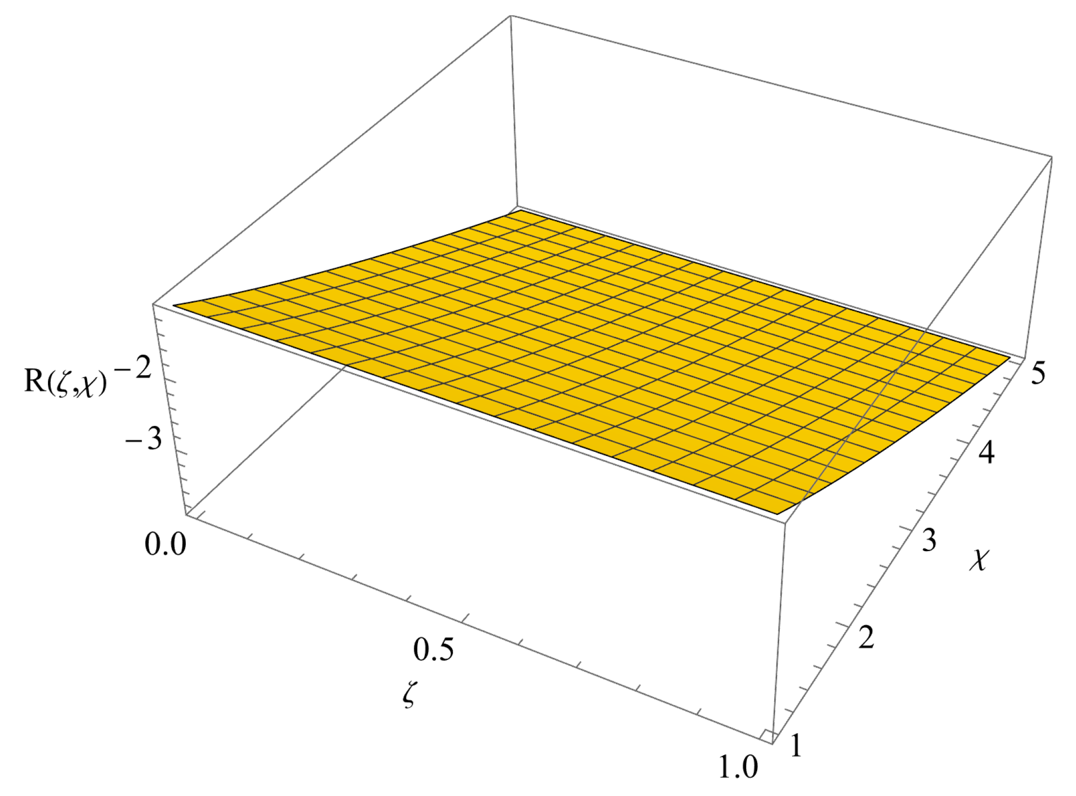
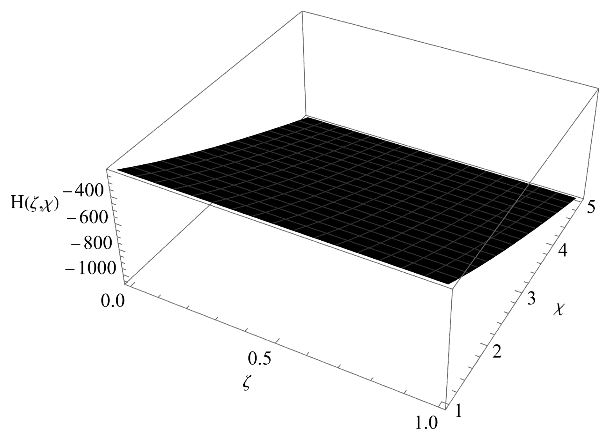
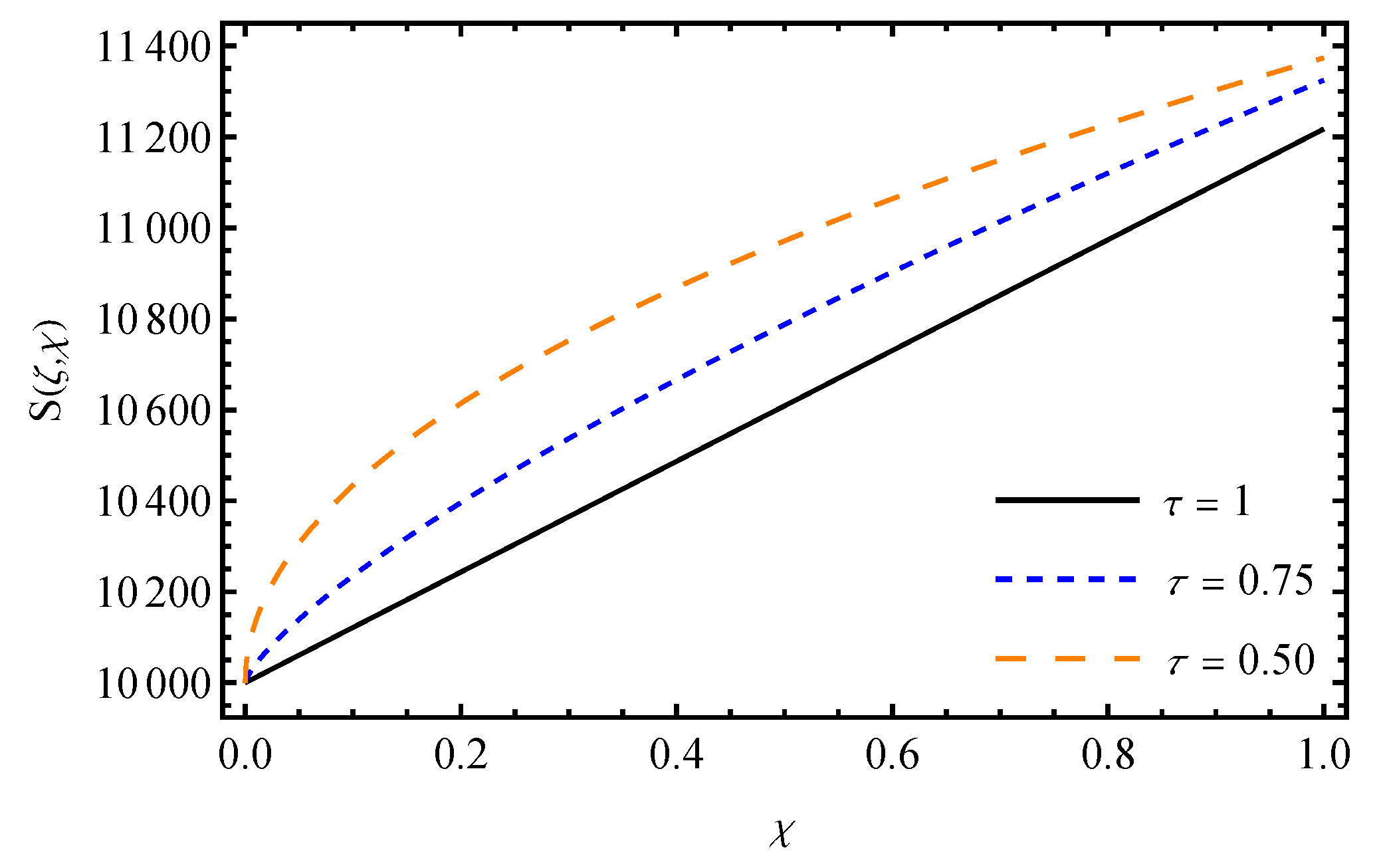
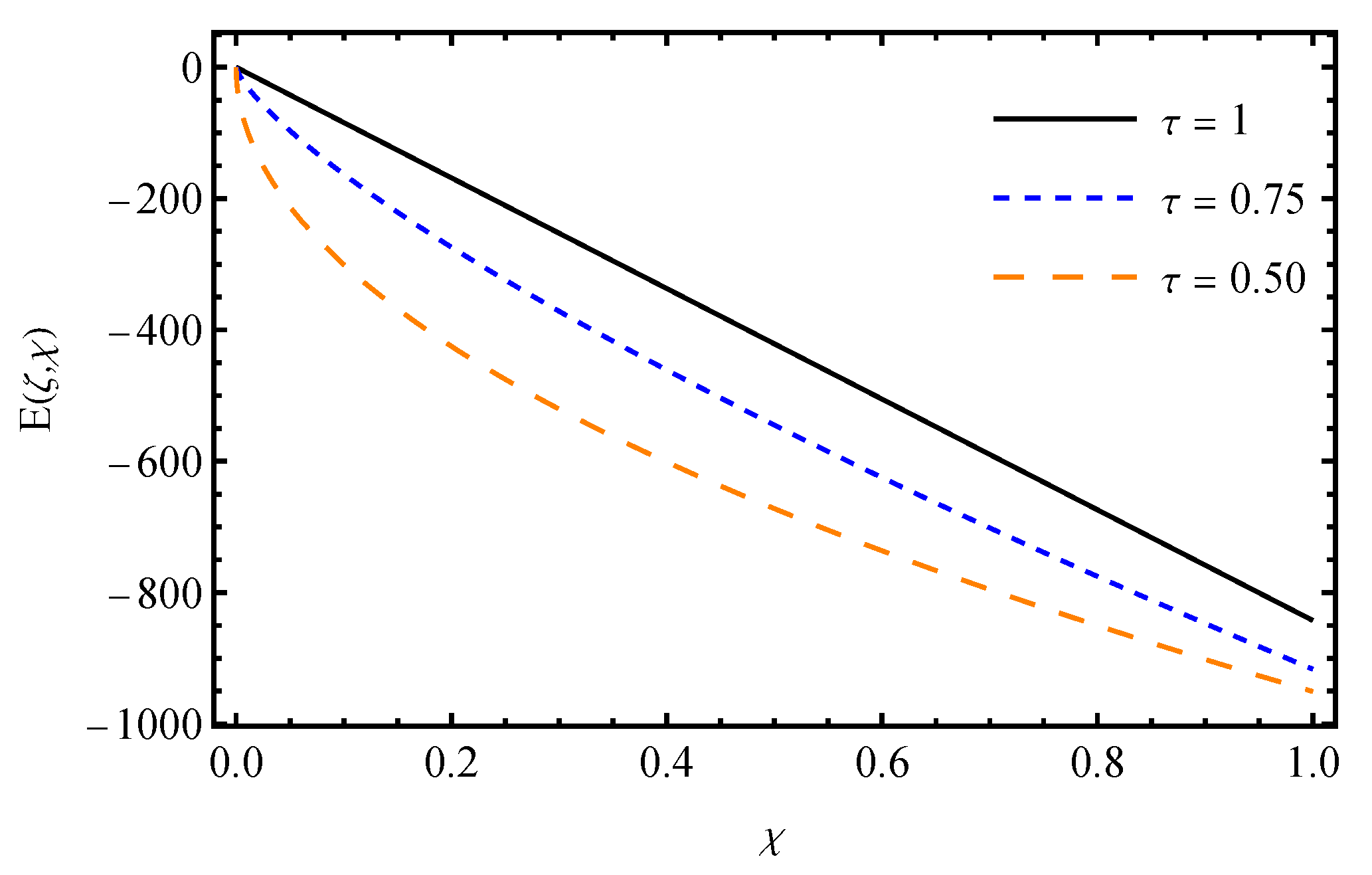
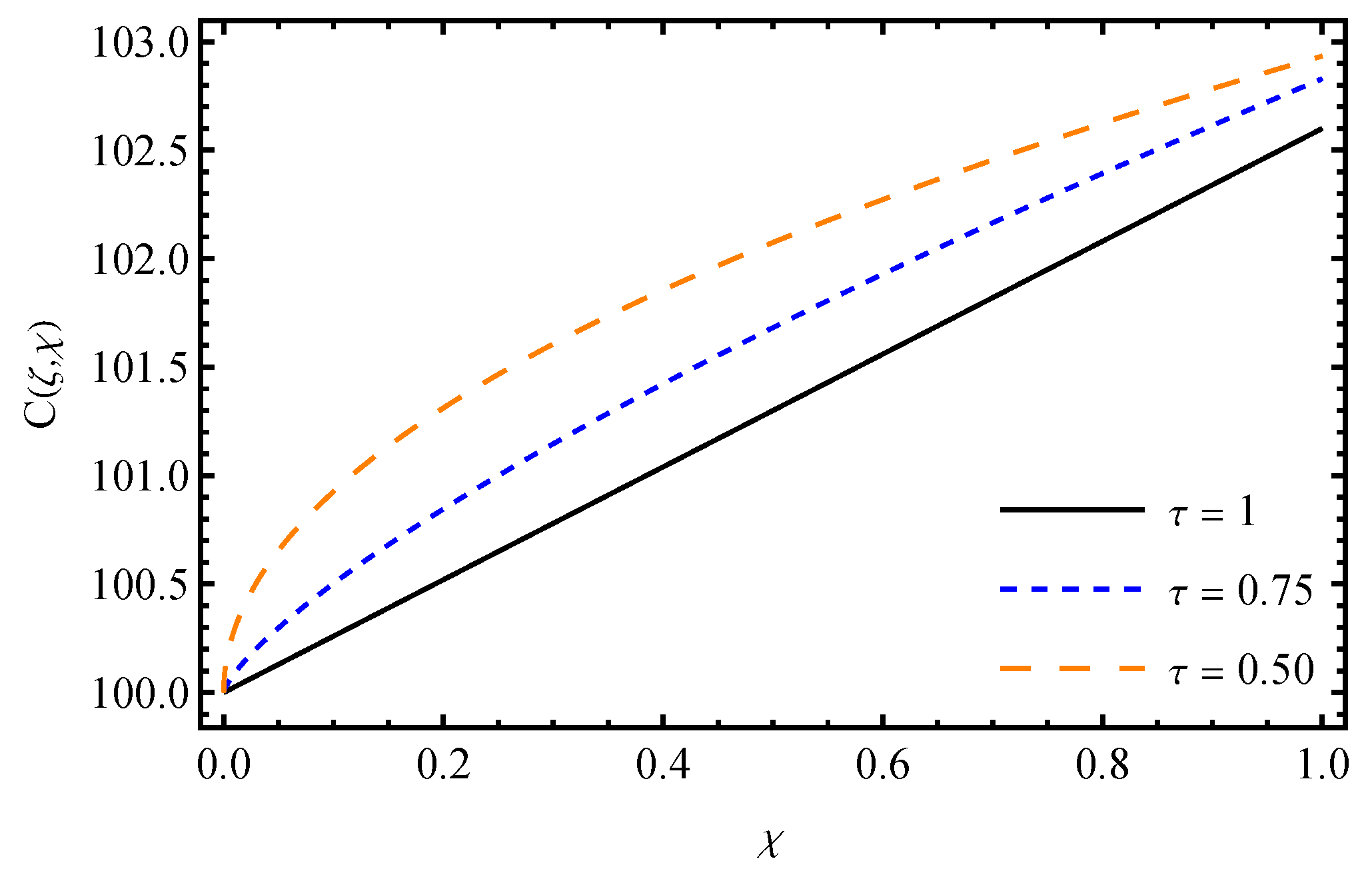
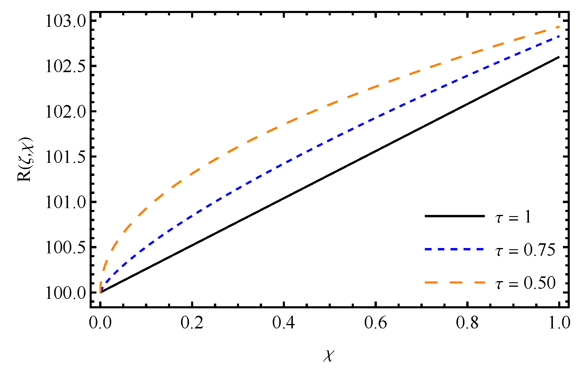
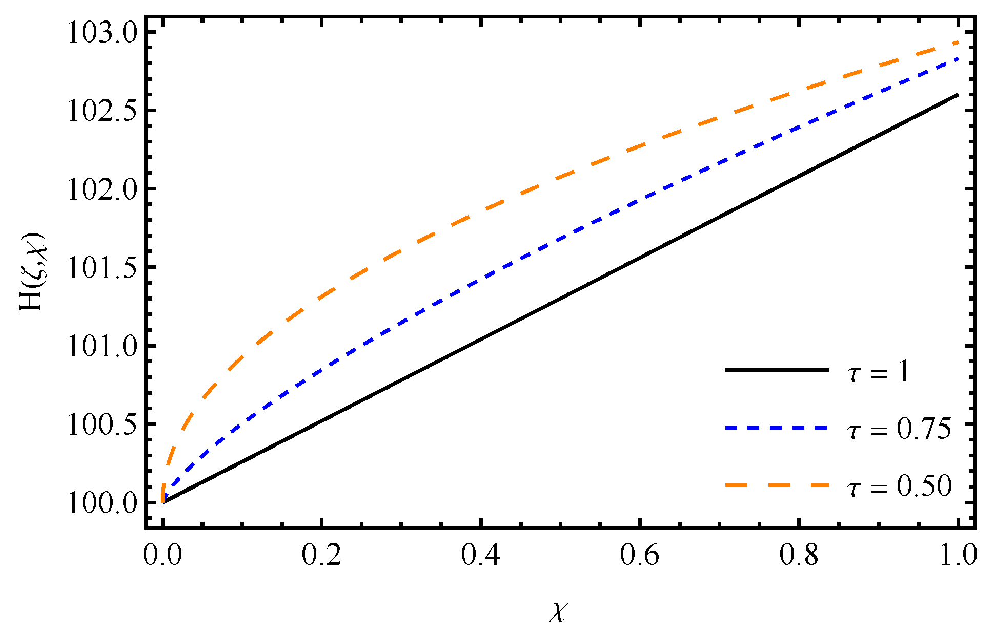
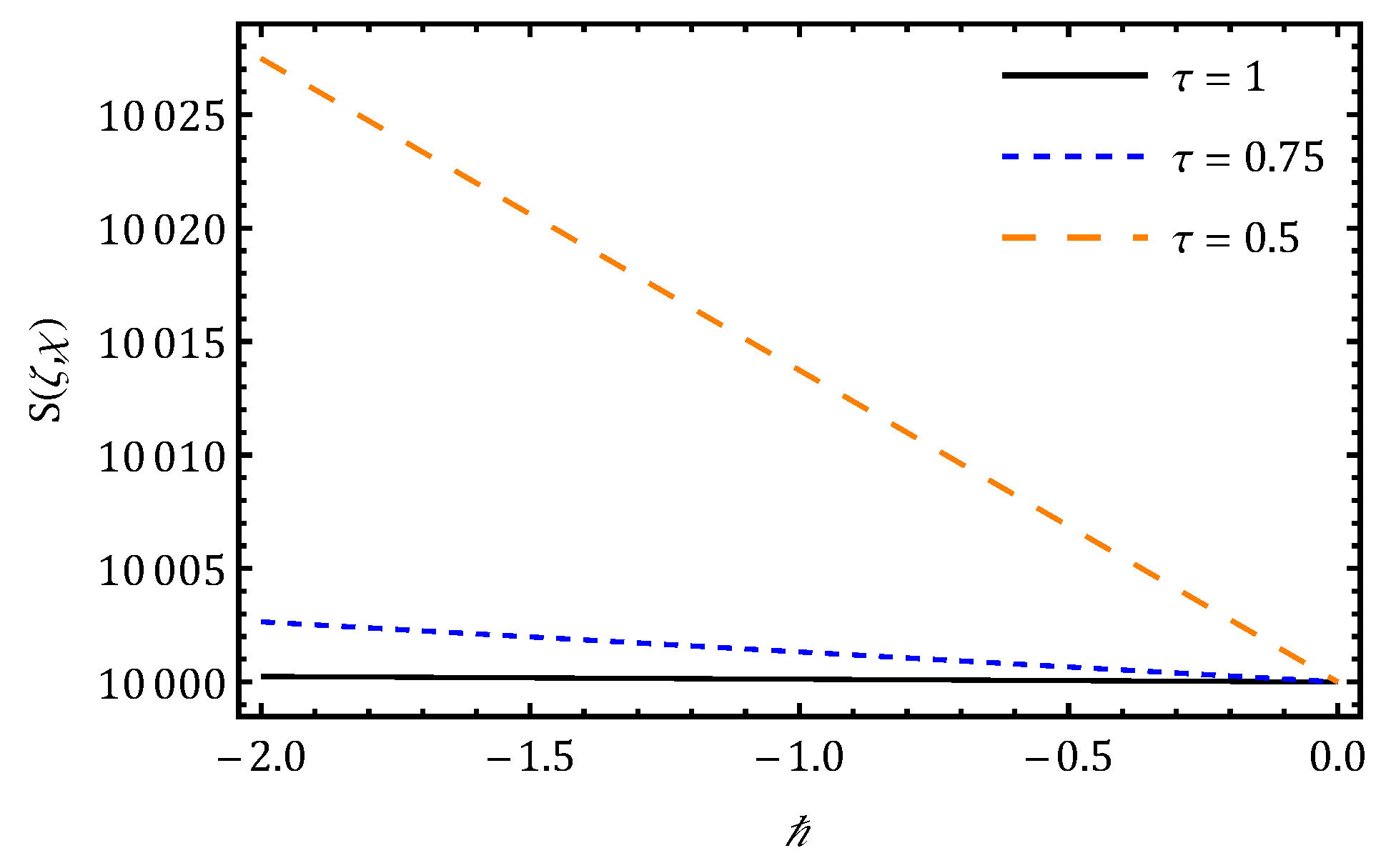
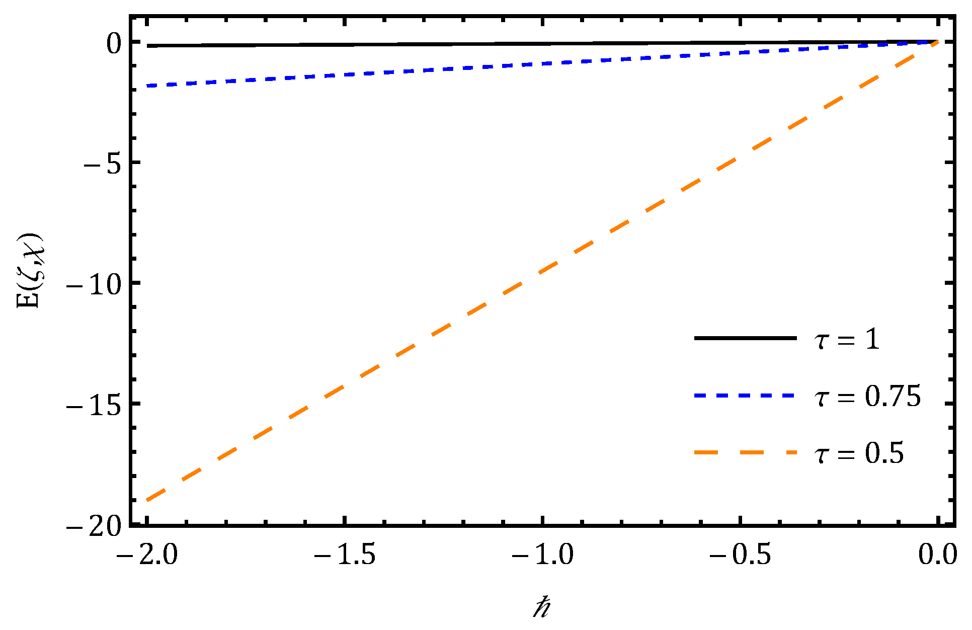
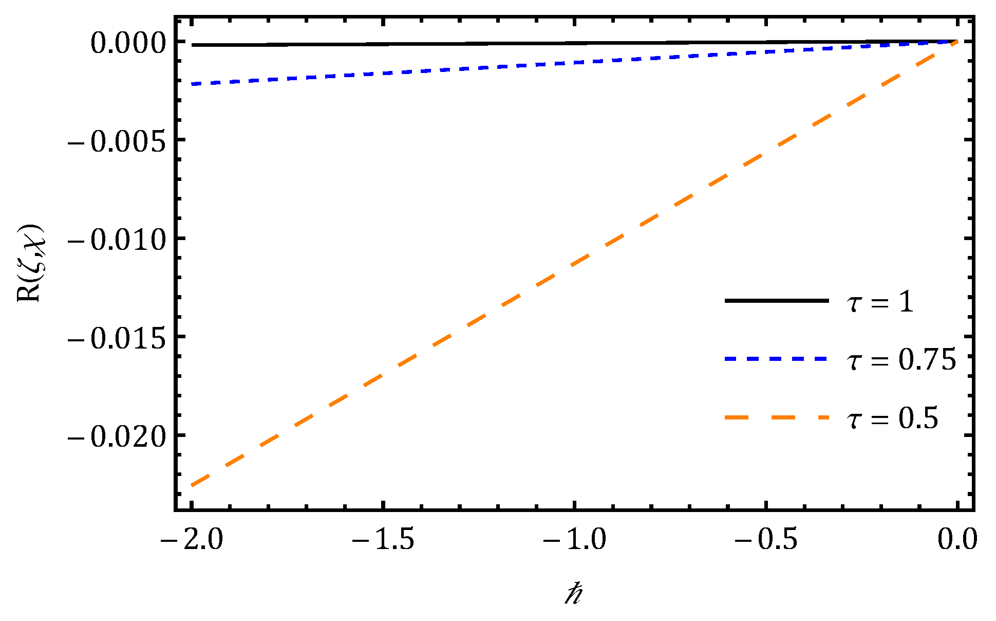
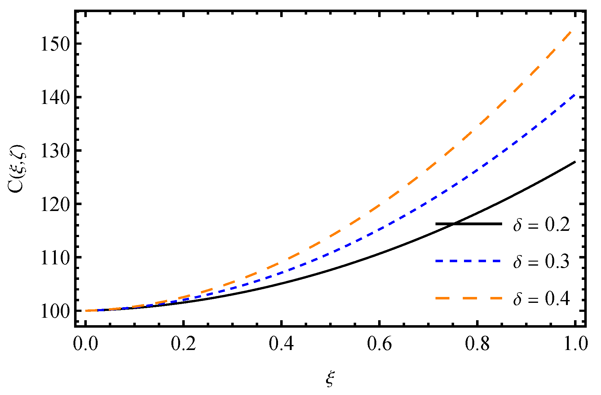
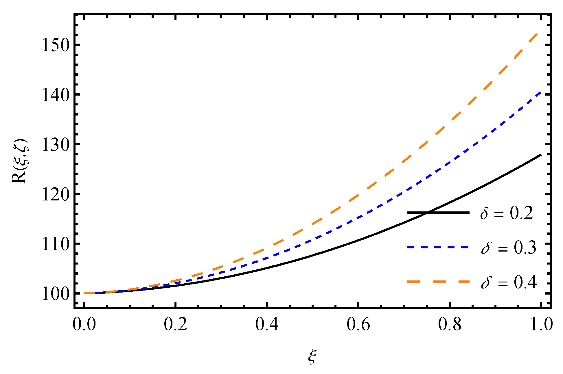
Moreover, the results are presented in a series form with 3D graphs, which determine the accuracy of the projected approach. Figure 1, Figure 2, Figure 3, Figure 4 and Figure 5 portrays the 3D behaviour of individuals over time. Figure 6, Figure 7, Figure 8, Figure 9 and Figure 10 demonstrate the system’s behavior at various fractional orders ( τ = 1, 0.75, 0.50). The results suggest that decreasing the fractional order enhances the memory impact in corruption dynamics. Specifically, the fall of vulnerable people slows, but the corrupted population remains at greater levels for a longer duration. Anti-corruption efforts may be less effective when significant historical variables are present, as seen by the progressive increase in recovered and honest persons. These patterns show that the fractional-order technique, as opposed to typical integer-order models, provides a more realistic portrayal of long-term persistence and delayed responses in corruption processes. Figure 11, Figure 12, Figure 13, Figure 14 and Figure 15 depicts the behavior of curves for various non-integer values and feasible values, and the resultant series solutions swiftly converge. The effect of the parameter δ on behavior of system 6 is portrayed in Figure 16 and Figure 17. Equation (16) demonstrates how an increase in δ speeds up the spread of corruption and rises the number of corrupted individuals. A higher δ shows delayed corrective reactions in Equation (17) by slightly increasing the restored population. These findings highlight that δ plays a vital role in shaping corruption dynamics, and reducing this rate through preventive strategies can effectively limit corruption instances. Based on actual findings, we discovered that using non-integer derivatives allows us to better reflect the structure of corruption dynamics, and the q-HATM based on the projected model yields the best results. The distinctive performance of the computational q-HATM is observed for each category of the non-linear mathematical model under consideration.

8. Conclusions

In this study, we successfully develop a precise and effective mathematical model to understand the dynamics of corruption using q-HATM. It introduces a non-linear deterministic mathematical model employing fractional-order calculus to comprehensively analyze and capture the dynamics of corruption levels within a population. The model captures the complex dynamics of corruption with more accuracy and less processing work by dividing the individuals into five distinct categories and using a time-fractional technique. The results, including 3D plots, uniqueness, and convergence analysis, demonstrate that the projected approach effectively deals with non-linear systems. The findings demonstrate that this technique is systematic, economical, and highly trustworthy for modeling complicated real-world processes, making a substantial contribution to the fields of corruption dynamics and fractional-order modeling. The considered technique provides a substantial leap forward in the solution of non-linear physical systems. It offers a series solution over a broad acceptable domain, ensuring quick convergence and ease in application. We analyze the given model’s stability and examine the equilibrium points, elucidating the conditions necessary for a stable solution. The authors conduct a comprehensive stability analysis of the projected model to understand how corruption can be eliminated or become endemic within a population. In this study, we utilized the Caputo fractional derivative in a time-dependent model. The results were obtained in series form using the projected technique, and graphs were generated to depict the behavior of the model. The projected technique solves the non-linear issue without the use of discretization, perturbation, or transformation. The results obtained from q-HATM possess significant physical relevance, since they can better represent natural phenomena than typical integer-order techniques, resulting in a greater understanding of complex systems. The current study shows that the explored non-linear phenomena are strongly reliant on time history and time instant, and that fractional order calculus may be used to properly analyze them. Surface plots are used to depict approximate solutions, revealing a powerful method that may be extended to other types of PDEs with non-integer order that exist in mathematical physics. The current work assists researchers in studying the behavior of non-linear systems, which has highly intriguing and important implications. The instability of the equilibrium constraints portrays that a corruption-free state is highly fragile and can easily shift toward enhanced corruption when control measures weaken. This produces real social systems where minor policy lapses in governance can trigger numerous unethical characteristics. The results emphasize that lasting integrity requires continuous enforcement, and public accountability to block the system from reverting to unstable and corruption-prone conditions. Finally, we conclude that the proposed technique is more systematic, effective, precise, and used to analyze a wide range of non-linear problems in science and technology. In future work, we highlight that the model can be extended to incorporate stochastic formulations (to capture random fluctuations in corruption processes), spatial dynamics (to reflect regional or institutional heterogeneity), and data-driven parameter calibration (to improve empirical accuracy). Furthermore, we emphasize that such extensions can be applied in real-world anti-corruption strategies by allowing for policymakers to simulate the effects of preventive versus punitive measures, assess the impact of transparency and enforcement policies, and evaluate long-term outcomes under different socio-economic scenarios.

Author Contributions

Q.C.: formal analysis, software, writing, and methodology; K.N.: validation and methodology, writing—original draft, writing—review; D.G.P.: investigation—review and editing, and supervision; H.M.B.: methodology, resources, writing—review and editing. All authors have read and agreed to the published version of the manuscript.

Funding

The author K. Naveen is thankful to Ministry of Tribal Affairs, Government of India, for providing financial assistance in the form of Fellowship (Award No: 202324-NFST-KAR-00939).

Data Availability Statement

The original contributions presented in this study are included in the article. Further inquiries can be directed to the corresponding author.

Conflicts of Interest

The authors declare that they have no competing interests.

References

  1. Gweryina, R.I.; Kura, M.Y.; Okwu, E. An epidemiological model of corruption with immunity clause in Nigeria. World J. Model. Simul. 2019, 15, 262–275. [Google Scholar]
  2. World Bank. Helping Countries Combat Corruption: The Role of the World Bank; World Bank: Washington, DC, USA, 2020. [Google Scholar]
  3. Kaufmann, D. Myths and realities of governance and corruption. SSRN Electron. J. 2005, 829244. [Google Scholar] [CrossRef]
  4. Lehtinen, J.; Locatelli, G.; Sainati, T.; Artto, K.; Evans, B. The grand challenge: Effective anti-corruption measures in projects. Int. J. Proj. Manag. 2022, 40, 347–361. [Google Scholar] [CrossRef]
  5. Gibbon, E. Decline and Fall of the Roman Empire; BoD–Books on Demand; Strahan & Cadell: London, UK, 2024; Volume V. [Google Scholar]
  6. Corruption Transparency International. The Global Coalition Against Corruption. 2022. Available online: www.transparency.org/cpi (accessed on 1 January 2022).
  7. Ijewereme, O.B. Anatomy of corruption in the Nigerian public sector: Theoretical perspectives and some empirical explanations. Sage Open 2015, 5, 2158244015581188. [Google Scholar]
  8. Goel, R.K.; Nelson, M.A. Economic freedom versus political freedom: Cross–country influences on corruption. Aust. Econ. Perspect. 2005, 19, 19–42. [Google Scholar] [CrossRef]
  9. Dimant, E. The Antecedents and Effects of Corruption-A Reassessment of Current (Empirical) Findings; University Library of Munich: Munich, Germany, 2014. [Google Scholar]
  10. Fantaye, A.K.; Birhanu, Z.K. Mathematical Model and Analysis of Corruption Dynamics with Optimal Control. J. Appl. Math. 2022, 2022, 8073877. [Google Scholar] [CrossRef]
  11. Anjam, Y.N.; Aslam, M.I.; Cheema, S.A.; Munawar, S.; Saleem, N.; Rahman, M.U. Stability analysis of the corruption dynamics under fractional-order interventions. Nonlinear Eng. 2024, 13, 20220363. [Google Scholar] [CrossRef]
  12. Kilbas, A.A.; Srivastava, H.M.; Trujillo, J.J. Theory and Applications of Fractional Differential Equations; Elsevier: Amsterdam, The Netherlands, 2006; Volume 206. [Google Scholar]
  13. Miller, K.S.; Ross, B. An Introduction to the Fractional Calculus and Fractional Differential Equations; John Wiley & Sons, Inc.: New York, NY, USA, 1993. [Google Scholar]
  14. Podlubny, I. Fractional Differential Equations; Academic Press: New York, NY, USA, 1999. [Google Scholar]
  15. Cruz–Duarte, J.M.; Rosales-Garcia, J.; Correa-Cely, C.R.; Garcia–Perez, A.; Avina–Cervantes, J.G. A closed form expression for the Gaussian–based Caputo–Fabrizio fractional derivative for signal processing applications. Commun. Nonlinear Sci. Numer. Simul. 2018, 61, 138–148. [Google Scholar]
  16. Tarasov, V.E. General non-local electrodynamics: Equations and non-local effects. Ann. Phys. 2022, 445, 169082. [Google Scholar] [CrossRef]
  17. Zhang, Y.; Meerschaert, M.M. Particle tracking solutions of vector fractional differential equations: A review. HFCA 2019, 3, 275–285. [Google Scholar]
  18. Waheed, W.; Deng, G.; Liu, B. Discrete Laplacian operator and its applications in signal processing. IEEE Access 2020, 8, 89692–89707. [Google Scholar] [CrossRef]
  19. Naveen, K.; Mukhtar, S.; Mahnashi, A.M.; Shah, R.; Prakasha, D.G.; Archana, D.K. A robust technique to study fractional model describing economic and environmental mathematical system. Eng. Comput. 2025, 42, 1205–1224. [Google Scholar] [CrossRef]
  20. Kumar, C.V.D.; Prakasha, D.G.; Turki, N.B. Exploring the dynamics of fractional-order nonlinear dispersive wave system through homotopy technique. Open Phys. 2025, 23, 20250128. [Google Scholar] [CrossRef]
  21. Chethan, H.B.; Turki, N.B.; Prakasha, D.G. High performance computational approach to study model describing reversible two-step enzymatic reaction with time fractional derivative. Sci. Rep. 2024, 14, 21114. [Google Scholar] [CrossRef] [PubMed]
  22. Liao, S. Homotopy analysis method: A new analytical technique for nonlinear problems. Commun. Nonlinear Sci. Numer. Simul. 1997, 2, 95–100. [Google Scholar] [CrossRef]
  23. Singh, J.; Kumar, D.; Swaroop, R. Numerical solution of time-and space-fractional coupled Burgers’ equations via homotopy algorithm. Alex. Eng. J. 2016, 55, 1753–1763. [Google Scholar] [CrossRef]
  24. Veeresha, P.; Malagi, N.S.; Prakasha, D.G.; Baskonus, H.M. An efficient technique to analyze the fractional model of vector-borne diseases. Phys Scr. 2022, 97, 054004. [Google Scholar] [CrossRef]
  25. Naveen, K.; Prakasha, D.G.; Mofarreh, F.; Haseeb, A. A study on solutions of fractional order equal-width equation using novel approach. Mod. Phys. Lett. B 2025, 39, 2550058. [Google Scholar] [CrossRef]
  26. Qi, X.; Xu, C. An efficient numerical method to the stochastic fractional heat equation with random coefficients and fractionally integrated multiplicative noise. Fract. Calc. Appl. Anal. 2024, 27, 2754–2780. [Google Scholar] [CrossRef]
  27. Jarad, F.; Abdeljawad, T. A modified Laplace transform for certain generalized fractional operators. Results Nonlinear Anal. 2018, 1, 88–98. [Google Scholar]
  28. Magrenan, A.A. A new tool to study real dynamics: The convergence plane. Appl. Math. Comput. 2014, 248, 215–224. [Google Scholar] [CrossRef]
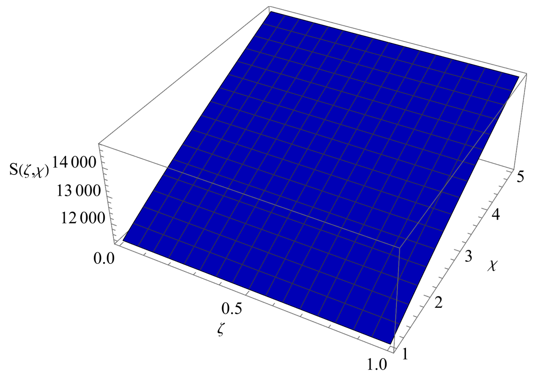
Figure 1. Nature of susceptible individuals S ( ξ ) over time.
Fractalfract 09 00666 g001
Figure 2. Nature of exposed individuals E ( ξ ) over time.
Fractalfract 09 00666 g002
Figure 3. Nature of corrupted individuals C ( ξ ) over time.
Fractalfract 09 00666 g003
Figure 4. Nature of recovered individuals R ( ξ ) over time.
Fractalfract 09 00666 g004
Figure 5. Nature of honest individuals H ( ξ ) over time.
Fractalfract 09 00666 g005
Figure 6. Nature of obtained results S ( ξ ) for projected application when ζ = 1 for distinct τ values over time.
Fractalfract 09 00666 g006
Figure 7. Behavior of the achieved results E ( ξ ) for projected application when ζ = 1 for distinct τ values over time.
Fractalfract 09 00666 g007
Figure 8. Nature of obtained outcomes C ( ξ ) for considered application when ζ = 1 for distinct τ values over time.
Fractalfract 09 00666 g008
Figure 9. Nature of achieved outcomes R ( ξ ) for considered problem when ζ = 1 , for distinct τ values over time.
Fractalfract 09 00666 g009
Figure 10. Behavior of the obtained results H ( ξ ) for projected application when ζ = 1 for distinct τ values over time.
Fractalfract 09 00666 g010
Figure 11. -curves for susceptible individuals S ( ξ ) over time.
Fractalfract 09 00666 g011
Figure 12. -curves for exposed individuals E ( ξ ) over time.
Fractalfract 09 00666 g012
Figure 13. -curves for corrupted individuals C ( ξ ) over time.
Fractalfract 09 00666 g013
Figure 14. -curves for recovered individuals R ( ξ ) over time.
Fractalfract 09 00666 g014
Figure 15. -curves for honest individuals H ( ξ ) over time.
Fractalfract 09 00666 g015
Figure 16. The effect of δ (rate at which persons exposed to corruption) for C ( ξ ) over time.
Fractalfract 09 00666 g016
Figure 17. The effect of δ (rate at which persons exposed to corruption) for R ( ξ ) over time.
Fractalfract 09 00666 g017
Disclaimer/Publisher’s Note: The statements, opinions and data contained in all publications are solely those of the individual author(s) and contributor(s) and not of MDPI and/or the editor(s). MDPI and/or the editor(s) disclaim responsibility for any injury to people or property resulting from any ideas, methods, instructions or products referred to in the content.