Analysis of a Finite Difference Method for a Time-Fractional Black–Scholes Equation

Abstract

The goal of this paper is to give an error analysis of a finite difference method for a time-fractional Black–Scholes equation with weakly singular solutions. The time Gerasimov-Caputo derivative is discretized by the L1 scheme on a graded mesh designed to compensate for the initial singularities, and a standard finite difference method is used for spatial discretization on a uniform mesh. A discrete comparison principle is presented for the fully discrete scheme, and stability and convergence of the scheme in maximum norm are established by constructing some appropriate barrier functions. Furthermore, an $\alpha$-robust pointwise error estimate of the fully discrete scheme on a uniform mesh is given. Finally, some numerical results are presented to show the sharpness of the error estimate.

1. Introduction

Black–Scholes equation (BSE) was first proposed by Black and Scholes [1] and Merton [2], which has wide applications in finance, such as options in derivatives, etc. The option price derived by the BSE model is under the assumption that the underlying asset follows the geometric Brownian motion and has constant volatility; thus, it fails to capture the significant movements or jumps over small time steps in a financial market [3].

In recent years, fractional differential equations (FDEs) have attracted extensive interest among researchers all over the world. Stynes et al. [4] first conducted an error analysis of the L1 scheme on graded mesh for a time-fractional diffusion equation with weakly singular solutions. Liao et al. [5] considered the L1 scheme on a general nonuniform mesh for a reaction-subdiffusion equation, and the convergence analysis is based on a discrete Gronwall inequality. Kopteva and Meng [6] established pointwise-in-time error estimates of the L1 scheme and Alikhanov’s scheme for the time-fractional diffusion equation, and later the analysis was extended to the L2 scheme in work [7]. Jin et al. [8] gave an extensive literature review on numerical methods for time-fractional evolution equations with nonsmooth data. In a series of papers, Yang and Zhang [9,10,11] investigated the convergence of the collocation method and finite volume method for subdiffusion equations. For the numerical approximation and analysis of quasilinear subdiffusion equations, we have noted two recent papers; see [12,13]. As FDEs involve the fractional derivatives, which have the properties of non-locality and long memory; thus, FDE-based models are proposed in the financial field. The following time-fractional BSE was proposed in [14]:

$${\displaystyle \frac{{\partial }^{\mathit{\alpha }}\mathit{w}}{\partial {\mathit{\tau }}^{\mathit{\alpha }}}}+{\displaystyle \frac{1}{2}}{\mathit{\sigma }}^2{\mathit{S}}^2{\displaystyle \frac{{\partial }^2\mathit{w}}{\partial {\mathit{S}}^2}}+\mathit{r}\mathit{S}{\displaystyle \frac{{\partial }^2\mathit{w}}{\partial \mathit{S}}}-\mathit{r}\mathit{w}=0,(\mathit{S},\mathit{\tau })\in (0,\infty )\times [0,\mathit{T}),$$

(1)

subject to terminal condition

$$\mathit{w}(\mathit{S},\mathit{T})=\tilde{\mathit{h}}\left(\mathit{S}\right),\mathit{S}\in (0,\infty ),$$

(2)

and boundary conditions

$$\mathit{w}(0,\mathit{\tau })=\tilde{\mathit{p}}\left(\mathit{\tau }\right),\underset{\mathit{S}\to \infty }{lim}\mathit{w}(\mathit{S},\mathit{\tau })=\tilde{\mathit{q}}\left(\mathit{\tau }\right),\mathit{\tau }\in [0,\mathit{T}],$$

(3)

where $\mathit{\sigma }$ is the volatility of the underlying asset, $0<\mathit{\alpha }<1$, r is the risk-free interest rate, T is the maturity date of the European option, and ${\displaystyle \frac{{\partial }^{\mathit{\alpha }}\mathit{w}}{\partial {\mathit{\tau }}^{\mathit{\alpha }}}}$ denotes the modified right Riemann–Liouville derivative which is defined by the following:

$$\begin{array}{c}\hfill {\displaystyle \frac{{\partial }^{\mathit{\alpha }}\mathit{w}}{\partial {\mathit{\tau }}^{\mathit{\alpha }}}}={\displaystyle \frac{1}{\Gamma (1-\mathit{\alpha })}}{\displaystyle \frac{\mathit{d}}{\mathit{d}\mathit{t}}}{\int }_{\mathit{\tau }}^{\mathit{T}}{\displaystyle \frac{\mathit{w}(\mathit{S},\mathit{\xi })-\mathit{w}(\mathit{S},\mathit{T})}{{(\mathit{\xi }-\mathit{\tau })}^{\mathit{\alpha }}}}\mathit{d}\mathit{\xi }.\end{array}$$

Let $\mathit{t}=\mathit{T}-\mathit{\tau }$, $\mathit{x}=ln\mathit{S}$, and $\mathit{u}(\mathit{x},\mathit{t})=\mathit{w}({\mathit{e}}^{\mathit{x}},\mathit{T}-\mathit{t})$, assume $\mathit{u}\in \mathit{C}[0,\mathit{T}]\cap {\mathit{C}}^1(0,\mathit{T}]$, after transformation, the model (1)–(3) can be rewritten as the following initial-boundary value problem [15]:

$$\begin{array}{cc}\hfill & {\mathit{D}}_{\mathit{t}}^{\mathit{\alpha }}\mathit{u}-{\displaystyle \frac{1}{2}}{\mathit{\sigma }}^2{\displaystyle \frac{{\partial }^2\mathit{u}}{\partial {\mathit{x}}^2}}-(\mathit{r}-{\displaystyle \frac{1}{2}}{\mathit{\sigma }}^2){\displaystyle \frac{\partial \mathit{u}}{\partial \mathit{x}}}+\mathit{r}\mathit{u}=0,(\mathit{x},\mathit{t})\in (-\infty ,+\infty )\times (0,\mathit{T}],\hfill \end{array}$$

(4)

$$\begin{array}{cc}\hfill & \mathit{u}(\mathit{x},0)=\mathit{h}\left(\mathit{x}\right),\mathit{x}\in (-\infty ,+\infty ),\hfill \end{array}$$

(5)

$$\begin{array}{cc}\hfill & \underset{\mathit{x}\to -\infty }{lim}\mathit{u}(\mathit{x},\mathit{t})=\mathit{p}\left(\mathit{t}\right),\underset{\mathit{x}\to +\infty }{lim}\mathit{u}(\mathit{x},\mathit{t})=\mathit{q}\left(\mathit{t}\right)\mathit{t}\in [0,\mathit{T}],\hfill \end{array}$$

(6)

where ${\mathit{D}}_{\mathit{t}}^{\mathit{\alpha }}\mathit{u}$ is the Gerasimov-Caputo derivative of order $\mathit{\alpha }\in (0,1)$ with respect to t. It is defined as follows:

$$\begin{array}{c}\hfill {\mathit{D}}_{\mathit{t}}^{\mathit{\alpha }}\mathit{u}(\mathit{x},\mathit{t})={\int }_0^{\mathit{t}}{\displaystyle \frac{{(\mathit{t}-\mathit{s})}^{-\mathit{\alpha }}}{\Gamma (1-\mathit{\alpha })}}{\displaystyle \frac{\partial \mathit{u}(\mathit{x},\mathit{s})}{\partial \mathit{s}}}\mathrm{d}\mathit{s}.\end{array}$$

(7)

To numerically solve the option price problem, usually the unbounded spatial domain is truncated into a bounded domain $(-X,X)$, where in practice, $X>0$ is large enough so that the truncated boundary in the price scale S is three to four times the strike price [16]. Without loss of generality, in this paper, we consider the following model problem:

$$\begin{array}{cc}\hfill & {\mathit{D}}_{\mathit{t}}^{\mathit{\alpha }}\mathit{u}-\mathit{a}{\displaystyle \frac{{\partial }^2\mathit{u}}{\partial {\mathit{x}}^2}}-\mathit{b}{\displaystyle \frac{\partial \mathit{u}}{\partial \mathit{x}}}+\mathit{c}\mathit{u}=\mathit{f}(\mathit{x},\mathit{t}),(\mathit{x},\mathit{t})\in \Omega \times (0,\mathit{T}],\hfill \end{array}$$

(8)

$$\begin{array}{cc}\hfill & \mathit{u}(\mathit{x},0)=\mathit{\varphi }\left(\mathit{x}\right),\mathit{x}\in \Omega ,\hfill \end{array}$$

(9)

$$\begin{array}{cc}\hfill & \mathit{u}(\mathit{x},\mathit{t})=0,(\mathit{x},\mathit{t})\in \partial \Omega \times (0,\mathit{T}],\hfill \end{array}$$

(10)

where a, b, and c are constants satisfying $a>0$ and $c\ge 0$; $\Omega =(x_l,x_r)$; and f is a continuous function.

Zhang et al. [15] proposed a finite difference method for the model problem (8)–(10), but the error analysis is under sufficient solution regularity, while it is well-known that the solution typically exhibits some weak initial singularity for the time-fractional derivative problem [17]. Hence, the aim of this paper is to provide a detailed error analysis under the realistic assumption that the solution has weakly singular solutions. It should be noted that, recently, some papers have taken the weak singularity under consideration, such as [18,19,20]. The work [18] proposed a compact difference method for time-fractional BSE, and ref. [19] proposed two higher-order compact difference methods for time-fractional BSE; both of the two works used the L1 scheme for the discretization of the time-fractional derivative. The work [20] proposed a fast scheme with variable time steps for the time-fractional BSE, where they used Alikhanov’s scheme for approximation of the time-fractional derivative.

The main contributions of this paper are as follows:

• We employ the L1 scheme on a graded mesh to compensate for the weak singularity at initial time.
• A discrete comparison principle is established for the fully discrete scheme.
• Stability and convergence of the fully discrete scheme in maximum norm are presented by constructing some barrier functions.
• An $\alpha$-robust pointwise error estimate of the fully discrete scheme on a uniform mesh is established.

The paper is outlined as follows: In Section 2, we construct a finite difference scheme for the problem (8)–(10). A discrete comparison principle of the fully discrete scheme is given in Section 3, and based on it the stability of the fully discrete scheme is presented in Section 4 by constructing some appropriate barrier functions. The convergence of the fully discrete scheme in maximum norm is proved in Section 5. Section 6 is devoted to giving an $\alpha$-robust pointwise error estimate of the scheme on a uniform mesh. Some numerical results are presented in Section 7. Finally, the paper ends with a conclusion in Section 8.

Notation: Throughout the work, C denotes a generic constant, it may have different values in various contexts, but it is always independent of the mesh sizes.

2. A Finite Difference Scheme

Given two positive integers M and N, we partition the space and time intervals $[{\mathit{x}}_{\mathit{l}},{\mathit{x}}_{\mathit{r}}]$ and $[0,\mathit{T}]$ into M and N parts, respectively, with the mesh points ${\mathit{x}}_{\mathit{l}}={\mathit{x}}_0<{\mathit{x}}_1<\cdots <{\mathit{x}}_{\mathit{M}}={\mathit{x}}_{\mathit{r}}$ and $0={\mathit{t}}_0<{\mathit{t}}_1<\cdots <{\mathit{t}}_{\mathit{N}}=\mathit{T}$. In this paper, we choose ${\mathit{x}}_{\mathit{i}}={\mathit{x}}_0+\mathit{i}\mathit{h}$ for $0\le \mathit{i}\le \mathit{M}$ with spatial step size $\mathit{h}=({\mathit{x}}_{\mathit{r}}-{\mathit{x}}_{\mathit{l}})/\mathit{M}$ and ${\mathit{t}}_{\mathit{n}}=\mathit{T}{(\mathit{n}/\mathit{N})}^{\mathit{r}}$ for $0\le \mathit{n}\le \mathit{N}$, with $\mathit{r}\ge 1$ as the grading parameter which can be chosen by the user. We designate ${\mathit{\tau }}_{\mathit{n}}={\mathit{t}}_{\mathit{n}}-{\mathit{t}}_{\mathit{n}-1}$ for $\mathit{n}\ge 1$. We denote ${\mathit{u}}_{\mathit{i}}^{\mathit{n}}$ as the approximation of the exact solution $\mathit{u}({\mathit{x}}_{\mathit{i}},{\mathit{t}}_{\mathit{n}})$ for all admissible i and n.

For discretizations of the spatial derivatives ${\displaystyle \frac{{\partial }^2\mathit{u}}{\partial {\mathit{x}}^2}}$ and ${\displaystyle \frac{\partial \mathit{u}}{\partial \mathit{x}}}$, we use the well-known second-order central difference formulas, viz., calculated as follows:

$$\begin{array}{c}\hfill {\displaystyle \frac{{\partial }^2\mathit{u}({\mathit{x}}_{\mathit{i}},{\mathit{t}}_{\mathit{n}})}{\partial {\mathit{x}}^2}}\approx {\mathit{\delta }}_{\mathit{x}}^2{\mathit{u}}_{\mathit{i}}^{\mathit{n}}:={\displaystyle \frac{{\mathit{u}}_{\mathit{i}+1}^{\mathit{n}}-2{\mathit{u}}_{\mathit{i}}^{\mathit{n}}+{\mathit{u}}_{\mathit{i}-1}^{\mathit{n}}}{{\mathit{h}}^2}},\end{array}$$

and

$$\begin{array}{c}\hfill {\displaystyle \frac{\partial \mathit{u}({\mathit{x}}_{\mathit{i}},{\mathit{t}}_{\mathit{n}})}{\partial \mathit{x}}}\approx {\mathit{\delta }}_{\mathit{x}}{\mathit{u}}_{\mathit{i}}^{\mathit{n}}:={\displaystyle \frac{{\mathit{u}}_{\mathit{i}+1}^{\mathit{n}}-{\mathit{u}}_{\mathit{i}-1}^{\mathit{n}}}{2\mathit{h}}}.\end{array}$$

For the approximation of the Gerasimov-Caputo fractional derivative $D_t^{\alpha }u(x_i,t_n)$, a widely used method is the L1 scheme, which uses piecewise linear interpolation to approximate the solution (see the review article [21] for more details), written as follows:

$$\begin{array}{c}\hfill {\delta }_t^{\alpha }{u}_i^n:=d_{n,0}{u}_i^n-d_{n,n-1}{u}_i^0-\sum _{j=1}^{n-1}(d_{n,j-1}-d_{n,j})u_i^{n-j},\end{array}$$

where

$$\begin{array}{c}\hfill d_{n,j}={\displaystyle \frac{{(t_n-t_{n-j-1})}^{1-\alpha }-{(t_n-t_{n-j})}^{1-\alpha }}{\Gamma (2-\alpha ){\tau }_{n-j}}}\mathrm{for}0\le j\le n-1.\end{array}$$

Note that $d_{n,0}={\tau }_n^{-\alpha }/\Gamma (2-\alpha )$, and one can easily verify the following:

$$d_{n,j-1}>d_{n,j}\mathrm{for}\mathrm{all}\mathrm{admissible}n\mathrm{and}j$$

(11)

by the mean value theorem.

Now we have the following discrete problem to approximate the continuous problem (8)–(10):

$$\begin{array}{cc}\hfill & L_{M,N}{u}_i^n:={\delta }_t^{\alpha }{u}_i^n-a{\delta }_x^2{u}_i^n-b{\delta }_x{u}_i^n+c{u}_i^n=f(x_i,t_n)\mathrm{for}n=1,\cdots ,N,1\le i\le M-1,\hfill \end{array}$$

(12)

$$\begin{array}{cc}\hfill & u_i^0=\varphi \left(x_i\right)\mathrm{for}0\le i\le M,\hfill \end{array}$$

(13)

$$\begin{array}{cc}\hfill & u_0^n=0,u_M^n=0\mathrm{for}0<n\le N\hfill \end{array}$$

(14)

3. A Discrete Comparison Principle

In [22], the authors established a discrete comparison principle for a time-fractional diffusion problem. In the following theorem, we extend the discrete comparison principle to the discrete problem (12)–(13) with an extra convection term.

Theorem 1.

Suppose $f\ge 0$ and $\varphi \ge 0$. Then for small h, we have the following:

$$u_i^n\ge 0\mathrm{for}0\le i\le M,0\le n\le N.$$

Proof. 

We imitate the proof of ([22], Theorem 2.1). Suppose there are some i and n such that $u_i^n<0$. Let $\widehat{n}$ denote the minimal value of n for which there exists some i such that $u_i^{\widehat{n}}<0$. Then select $\widehat{i}$ for which $u_i^{\widehat{n}}\ge u_{\widehat{i}}^{\widehat{n}}$ holds for all i. It is clear that $u_{\widehat{i}}^{\widehat{n}}<0$; also from the boundary conditions $u_0^n=u_M^n=0$ and initial condition $u_i^0=\varphi \left(x_i\right)\ge 0$, we know that $1\le \widehat{i}\le M-1$ and $1\le \widehat{n}\le N$. Then from (12), one has the following:

$$\begin{array}{cc}\hfill \left[d_{\widehat{n},0}+{\displaystyle \frac{2a}{h^2}}+c\right]u_{\widehat{i}}^{\widehat{n}}=& \left({\displaystyle \frac{a}{h^2}}+{\displaystyle \frac{b}{2h}}\right)u_{\widehat{i}+1}^{\widehat{n}}+\left({\displaystyle \frac{a}{h^2}}-{\displaystyle \frac{b}{2h}}\right)u_{\widehat{i}-1}^{\widehat{n}}+f(x_{\widehat{i}},t_{\widehat{n}})\hfill \\ \hfill & +d_{\widehat{n},\widehat{n}-1}{u}_{\widehat{i}}^0+\sum _{j=1}^{\widehat{n}-1}(d_{\widehat{n},j-1}-d_{\widehat{n},j})u_{\widehat{i}}^{\widehat{n}-j}.\hfill \end{array}$$

(15)

Now by the definition of $\widehat{n}$, one has $u_i^n\ge 0$ for all $n<\widehat{n}$ and all i. Also one has $u_i^{\widehat{n}}\ge u_{\widehat{i}}^{\widehat{n}}$ for all i, owing to the selection of $\widehat{i}$. Using these inequalities and $a>0$, for small h, from (15) we have the following:

$$\begin{array}{cc}\hfill \left[d_{\widehat{n},0}+{\displaystyle \frac{2a}{h^2}}+c\right]u_{\widehat{i}}^{\widehat{n}}\ge & \left({\displaystyle \frac{a}{h^2}}+{\displaystyle \frac{b}{2h}}\right)u_{\widehat{i}}^{\widehat{n}}+\left({\displaystyle \frac{a}{h^2}}-{\displaystyle \frac{b}{2h}}\right)u_{\widehat{i}}^{\widehat{n}}+f(x_{\widehat{i}},t_{\widehat{n}})\hfill \\ \hfill =& {\displaystyle \frac{2a}{h^2}}{u}_{\widehat{i}}^{\widehat{n}}+f(x_{\widehat{i}},t_{\widehat{n}}),\hfill \end{array}$$

(16)

which reduces to

$$\left[d_{\widehat{n},0}+c\right]u_{\widehat{i}}^{\widehat{n}}\ge f(x_{\widehat{i}},t_{\widehat{n}}).$$

Then by $c\ge 0$, $d_{\widehat{n},0}>0$, $f\ge 0$, one concludes that $u_{\widehat{i}}^{\widehat{n}}\ge 0$, which contradicts the assumption that $u_{\widehat{i}}^{\widehat{n}}<0$. Thus the lemma is true. □

4. A Barrier Function and Stability

We define the positive stability multipliers as follows:

$$\begin{array}{c}\hfill {\theta }_{n,n}=1,{\theta }_{n,j}=\sum _{k=1}^{n-j}{d}_{n-j,0}^{-1}(d_{n,k-1}-d_{n,k}){\theta }_{n-k,j}\mathrm{for}1\le j\le n-1.\end{array}$$

From Lemma 2.3 [23], we have the following lemma.

Lemma 1.

For any mesh function ${\left\{{\varphi }^j\right\}}_{j=0}^N$, set ${\eta }^0={\varphi }^0$, and ${\eta }^n={\varphi }^0+d_{n,0}^{-1}{\sum }_{j=1}^n{\theta }_{n,j}{\varphi }^j$ for $n=1,\cdots ,N$. Then one has the following:

$$\begin{array}{c}\hfill {\delta }_t^{\alpha }{\eta }^n={\varphi }^n\mathrm{for}n=1,\cdots ,N.\end{array}$$

For the properties of the stability multipliers, from ([24], Corollary 5.4), we have the following:

Lemma 2.

For $n=1,\cdots ,N$, one has the following:

$$\begin{array}{c}\hfill d_{n,0}^{-1}\sum _{j=1}^n{\theta }_{n,j}\le {\displaystyle \frac{t_n^{\alpha }}{\Gamma (1+\alpha )}}.\end{array}$$

For any mesh function ${\left\{v_i\right\}}_{i=0}^M$, we define the following:

$${\parallel v\parallel }_{\infty }:=\underset{0\le i\le M}{max}\left|v_i\right|.$$

Then we have the following stability theorem:

Theorem 2.

For the solution of the discrete problem (12)–(13), one has, for $n=1,\cdots ,N$, the following:

$$\begin{array}{c}\hfill \parallel u^n{\parallel }_{\infty }\le \parallel u^0{\parallel }_{\infty }+d_{n,0}^{-1}\sum _{j=1}^n{\theta }_{n,j}\parallel f^j{\parallel }_{\infty }\le \parallel u^0{\parallel }_{\infty }+{\displaystyle \frac{t_n^{\alpha }}{\Gamma (1+\alpha )}}\underset{1\le j\le n}{max}{\parallel f^j\parallel }_{\infty }.\end{array}$$

Proof. 

We construct a barrier function $B_i^n$ as follows: set $B_0^n=B_M^n=0$ for all n, and set $B_i^0={\parallel u^0\parallel }_{\infty }$, $B_i^n=\parallel u^0{\parallel }_{\infty }+d_{n,0}^{-1}{\sum }_{j=1}^n{\theta }_{n,j}{\parallel f^j\parallel }_{\infty }$ for $i=1,\cdots ,M-1$. Then using Lemma 1 and $c\ge 0$, we have the following:

$$\begin{array}{c}\hfill L_{M,N}{B}_i^n={\delta }_t^{\alpha }{B}_i^n+c{B}_i^n={\parallel f^n\parallel }_{\infty }+c{B}_i^n\ge f(x_i,t_n).\end{array}$$

Thus, by the discrete comparison principle, one has $u_i^n\le B_i^n$. Similarly, using $\parallel f^n{\parallel }_{\infty }\ge -f(x_i,t_n)$, we obtain $-u_i^n\le B_i^n$. Hence, one has $|u_i^n|\le B_i^n$ for all i and n. On the other hand, one has the following:

$$\begin{array}{cc}\hfill B_i^n& =\parallel u^0{\parallel }_{\infty }+d_{n,0}^{-1}\sum _{j=1}^n{\theta }_{n,j}{\parallel f^j\parallel }_{\infty }\hfill \\ \hfill & \le \parallel u^0{\parallel }_{\infty }+\underset{1\le j\le n}{max}{\parallel f^j\parallel }_{\infty }\left(d_{n,0}^{-1}\sum _{j=1}^n{\theta }_{n,j}\right)\hfill \\ \hfill & \le \parallel u^0{\parallel }_{\infty }+{\displaystyle \frac{t_n^{\alpha }}{\Gamma (1+\alpha )}}\underset{1\le j\le n}{max}{\parallel f^j\parallel }_{\infty },\hfill \end{array}$$

where we have used Lemma 2 to deduce the last inequality. Clearly, $\parallel u^n{\parallel }_{\infty }\le {\parallel B^n\parallel }_{\infty }$, the proof is completed. □

5. Convergence

We first need a lemma on the truncation error of L1 scheme.

Lemma 3

([6], Lemma 3.4). Assume that $|{\partial }_t^{l}u\left(t\right)|\le C{t}^{\alpha -l}$ for $l=0,1,2$. Then we obtain the following:

$$\begin{array}{c}\hfill |D_t^{\alpha }u\left(t_n\right)-{\delta }_t^{\alpha }u\left(t_n\right)|\le C{(t_1/t_n)}^{min\{\alpha +1,(2-\alpha )/r\}},n=1,\cdots ,N.\end{array}$$

Set the following:

$${\mathcal{N}}_{\gamma }^n:=\left\{\begin{array}{cc}{t}_1{t}_n^{\alpha -1}\hfill & \mathrm{if}\gamma >0,\hfill \\ t_1{t}_n^{\alpha -1}[1+ln(t_n/t_1)]\hfill & \mathrm{if}\gamma =0,\hfill \\ t_1{t}_n^{\alpha -1}{(t_1/t_n)}^{\gamma }\hfill & \mathrm{if}\gamma <0.\hfill \end{array}\right.$$

(17)

Then the following lemma is valid:

Lemma 4

([25], Lemma 2.5). Set ${\psi }^0=0$ and the following:

$${\psi }^n=d_{n,0}^{-1}\sum _{j=1}^n{\theta }_{n,j}{(t_1/t_j)}^{\gamma +1}\mathrm{for}n=1,\cdots ,N.$$

Then we obtain the following:

$${\psi }^n\le C{\mathcal{N}}_{\gamma }^n\mathrm{for}n=1,\cdots ,N,$$

where C is a positive constant.

Now we obtain the following convergence result:

Theorem 3.

Let $e_i^n:=u(x_i,t_n)-u_i^n$. Then one has the following:

$$\parallel e^n{\parallel }_{\infty }\le C(h^2+{\mathcal{E}}_N^n),n=1,\cdots ,N,$$

where

$${\mathcal{E}}_N^n:=\left\{\begin{array}{cc}{N}^{-r}{t}_n^{\alpha -1}\hfill & \mathit{if}1\le r<2-\alpha ,\hfill \\ N^{\alpha -2}{t}_n^{\alpha -1}[1+ln(t_n/t_1)]\hfill & \mathit{if}r=2-\alpha ,\hfill \\ N^{\alpha -2}{t}_n^{\alpha -(2-\alpha )/r}\hfill & \mathit{if}r>2-\alpha .\hfill \end{array}\right.$$

Proof. 

One has $L_{M,N}{e}_i^n=r_i^n$, where $r_i^n$ is the truncation error. As the spatial truncation error is second-order, from Lemma 3, we know that $\parallel r^n{\parallel }_{\infty }\le C\left(h^2+{(t_1/t_n)}^{min\{\alpha +1,(2-\alpha )/r\}}\right)$. Then similar as the proof of Theorem 2, noting that $e^0=0$, we have the following:

$$\begin{array}{cc}\hfill \parallel e^n{\parallel }_{\infty }& \le d_{n,0}^{-1}\sum _{j=1}^n{\theta }_{n,j}{\parallel r^j\parallel }_{\infty }\hfill \\ \hfill & \le C{d}_{n,0}^{-1}\sum _{j=1}^n{\theta }_{n,j}{h}^2+C{d}_{n,0}^{-1}\sum _{j=1}^n{\theta }_{n,j}{(t_1/t_j)}^{min\{\alpha +1,(2-\alpha )/r\}}\hfill \\ \hfill & \le C{h}^2+C{\mathcal{N}}_{\gamma }^n,\hfill \end{array}$$

(18)

where $\gamma :=min\{\alpha +1,(2-\alpha )/r\}-1$ and we have used Lemmas 2 and 4 to obtain the last inequality. It remains to prove that ${\mathcal{N}}_{\gamma }^n\le C{\mathcal{E}}_N^n$.

Case 1: $1\le r<2-\alpha$. Now $\gamma >0$, using $t_1=T{N}^{-r}$, one has ${\mathcal{N}}_{\gamma }^n=t_1{t}_n^{\alpha -1}\le C{N}^{-r}{t}_n^{\alpha -1}$.

Case 2: $r=2-\alpha$. Now $\gamma =0$, then ${\mathcal{N}}_{\gamma }^n=t_1{t}_n^{\alpha -1}[1+ln(t_n/t_1)]\le C{N}^{\alpha -2}{t}_n^{\alpha -1}[1+ln(t_n/t_1)]$ using $t_1=T{N}^{-r}$.

Case 3: $r>2-\alpha$. Now $\gamma <0$, then ${\mathcal{N}}_{\gamma }^n=t_1{t}_n^{\alpha -1}{(t_1/t_n)}^{(2-\alpha )/r-1}=t_1^{(2-\alpha )/r}{t}_n^{\alpha -(2-\alpha )/r}\le C{N}^{\alpha -2}{t}_n^{\alpha -(2-\alpha )/r}$ using $t_1=T{N}^{-r}$. Thus we obtain the desired result. □

6. $\mathbf{\alpha }$-Robust Pointwise Error Estimate on Uniform Mesh

One can see that there is a constant C in Lemma 4, which is based on the analysis of [6]. However, if one carefully checks the proof of ([6], Theorem 2.1), one can see that the constant C in Lemma 4 contains the factor $\Gamma (1-\alpha )$, which will blow up when $\alpha \to 1^{-}$. In this section, we give an $\alpha$-robust pointwise error estimate on a uniform mesh. We call the constant C $\alpha$-robust if it does not blow up when $\alpha \to 1^{-}$.

Now on uniform mesh, with the time step $\tau =T/N$, the L1 scheme becomes the following:

$$\begin{array}{c}\hfill {\delta }_t^{\alpha }{u}_i^n:=d_0{u}_i^n-d_{n-1}{u}_i^0-\sum _{j=1}^{n-1}(d_{j-1}-d_j)u_i^{n-j},\end{array}$$

where

$$\begin{array}{c}\hfill d_j={\displaystyle \frac{{(j+1)}^{1-\alpha }-j^{1-\alpha }}{\Gamma (2-\alpha ){\tau }^{\alpha }}}\mathrm{for}j\ge 0.\end{array}$$

Note that $d_0={\displaystyle \frac{1}{\Gamma (2-\alpha ){\tau }^{\alpha }}}$ and $d_j=d_{n,j}$ on uniform mesh. Now the stability multipliers becomes the following:

$$\begin{array}{c}\hfill {\theta }_0=1,{\theta }_j=d_0^{-1}\sum _{k=1}^j(d_{k-1}-d_k){\theta }_{j-k}\mathrm{for}j\ge 1.\end{array}$$

Note here ${\theta }_{n-j}={\theta }_{n,j}$ on uniform mesh. One can easily see that the definition of ${\theta }_j$ is the same as ([26], Equation (4.6)). Then we have the following:

Lemma 5

([26], Lemma 2). For $j\ge 1$, one has the following:

$$\begin{array}{c}\hfill {\theta }_j<{(j+1)}^{\alpha -1}.\end{array}$$

Given a positive integer n for $\beta \ge 0$, we define the following:

$$\begin{array}{c}\hfill K_{\beta ,n}:=\left\{\begin{array}{cc}1+{\displaystyle \frac{1-n^{1-\beta }}{\beta -1}}\hfill & \mathrm{if}\beta \ne 1,\hfill \\ 1+lnn\hfill & \mathrm{if}\beta =1.\hfill \end{array}\right.\end{array}$$

It is easy to verify that $K_{\beta ,n}$ is strictly decreasing for the variable $\beta$ and ${lim}_{\beta \to 1}{K}_{\beta ,n}=K_{1,n}$.

By Lemma 5, from ([27], Lemma 9), we have the following:

Lemma 6.

Let $\beta \ge 0$. For $n=1,\cdots$, one has the following:

$$\begin{array}{c}\hfill \sum _{j=1}^n{j}^{-\beta }{\theta }_{n-j}\le K_{\beta ,\lceil {\displaystyle \frac{n}{2}}\rceil }{\left({\displaystyle \frac{n}{2}}\right)}^{\alpha -1}+K_{1-\alpha ,\lceil {\displaystyle \frac{n}{2}}\rceil }{\left({\displaystyle \frac{n}{2}}\right)}^{-\beta }.\end{array}$$

On uniform mesh, i.e., $r=1$, from Lemma 3, the truncation error of L1 scheme is $|R_n:=D_t^{\alpha }u\left(t_n\right)-{\delta }_t^{\alpha }u\left(t_n\right)|\le C{n}^{-min\{\alpha +1,2-\alpha \}}$. Then we have the following lemma:

Lemma 7.

Let $\rho :=min\{\alpha +1,2-\alpha \}$. For $n=1,\cdots ,N$, one has the following:

$$\begin{array}{c}\hfill d_0^{-1}\sum _{j=1}^n{\theta }_{n-j}\left|R_j\right|\le C{K}_{\rho ,\lceil {\displaystyle \frac{n}{2}}\rceil }{\tau }^{\alpha }{n}^{\alpha -1}=C{K}_{\rho ,\lceil {\displaystyle \frac{n}{2}}\rceil }\tau t_n^{\alpha -1},\end{array}$$

where C is α-robust.

Proof. 

Note that $d_0^{-1}=\Gamma (2-\alpha ){\tau }^{\alpha }$, by Lemma 6, we obtain the following:

$$\begin{array}{cc}\hfill d_0^{-1}\sum _{j=1}^n{\theta }_{n-j}\left|R_j\right|& \le C{\tau }^{\alpha }\sum _{j=1}^n{\theta }_{n-j}{j}^{-\rho }\hfill \end{array}$$

(19)

$$\begin{array}{cc}\hfill & \le C{\tau }^{\alpha }\left[K_{\rho ,\lceil {\displaystyle \frac{n}{2}}\rceil }{\left({\displaystyle \frac{n}{2}}\right)}^{\alpha -1}+K_{1-\alpha ,\lceil {\displaystyle \frac{n}{2}}\rceil }{\left({\displaystyle \frac{n}{2}}\right)}^{-\rho }\right]\hfill \end{array}$$

(20)

$$\begin{array}{cc}\hfill & \le C{\tau }^{\alpha }\left[K_{\rho ,\lceil {\displaystyle \frac{n}{2}}\rceil }{n}^{\alpha -1}+n^{\alpha -\rho }\right],\hfill \end{array}$$

(21)

where we have used $K_{1-\alpha ,\lceil {\displaystyle \frac{n}{2}}\rceil }\le C{n}^{\alpha }$ to deduce the last inequality. Finally, noting that $\rho >1$ and $t_n=n\tau$, the desired result follows. □

Theorem 4.

Let $\rho :=min\{\alpha +1,2-\alpha \}$. For the errors $e_i^n:=u(x_i,t_n)-u_i^n$ on uniform mesh, one has the following:

$$\parallel e^n{\parallel }_{\infty }\le C(h^2+K_{\rho ,\lceil {\displaystyle \frac{n}{2}}\rceil }\tau t_n^{\alpha -1}),n=1,\cdots ,N,$$

where C is α-robust.

Proof. 

Following the proof of Theorem 3, substituting Lemma 7 into (18), one obtains the desired result. □

7. Numerical Experiments

Example 1.

Let $\Omega =(0,1)$, $T=1$, $a=1/32$, $b=0.05-a$, $c=0.05$. Suppose the problem (8)–(10) has an exact solution, written as follows:

$$u(x,t)=(1+t^{\alpha })x^2(1-x)$$

which exhibits a typical weak singularity at the initial time. The function f can be computed by (8).

We define $E_G:=\underset{1\le n\le N}{max}{\parallel u\left(t_n\right)-u^n\parallel }_{\infty }$ as global errors and $E_L:={\parallel u\left(t_N\right)-u^N\parallel }_{\infty }$ as local errors. As the spatial accuracy is well-known, here we just show the convergence in the time direction. To test the temporal accuracy, we take $M=\mathrm{10,000}$ to eliminate the contamination of the spatial errors.

Table 1. Global errors and orders of convergence for Example 1 when $r=1$.

N	$\mathit{\alpha }=0.3$			$\mathit{\alpha }=0.5$			$\mathit{\alpha }=0.7$
	${\mathit{E}}_{\mathit{G}}$	$\mathit{order}$		${\mathit{E}}_{\mathit{G}}$	$\mathit{order}$		${\mathit{E}}_{\mathit{G}}$	$\mathit{order}$
32	8.3580e-03			5.2216e-03			2.3272e-03
64	6.9637e-03	0.2633		3.7715e-03	0.4694		1.4534e-03	0.6792
128	5.7786e-03	0.2692		2.7078e-03	0.4780		9.0267e-04	0.6872
256	4.7781e-03	0.2743		1.9356e-03	0.4843		5.5871e-04	0.6921
512	3.9389e-03	0.2787		1.3793e-03	0.4889		3.4508e-04	0.6951

,

Table 2. Local errors and orders of convergence for Example 1 when $r=1$.

N	$\mathit{\alpha }=0.3$			$\mathit{\alpha }=0.5$			$\mathit{\alpha }=0.7$
	${\mathit{E}}_{\mathit{L}}$	$\mathit{order}$		${\mathit{E}}_{\mathit{L}}$	$\mathit{order}$		${\mathit{E}}_{\mathit{L}}$	$\mathit{order}$
32	3.7167e-04			6.1436e-04			8.1037e-04
64	1.8055e-04	1.0416		3.0158e-04	1.0265		4.1087e-04	0.9799
128	8.8394e-05	1.0304		1.4884e-04	1.0188		2.0783e-04	0.9833
256	4.3511e-05	1.0226		7.3738e-05	1.0133		1.0493e-04	0.9860
512	2.1501e-05	1.0170		3.6629e-05	1.0094		5.2890e-05	0.9883

,

Table 3. Global errors and orders of convergence for Example 1 when $r=2$.

N	$\mathit{\alpha }=0.3$			$\mathit{\alpha }=0.5$			$\mathit{\alpha }=0.7$
	${\mathit{E}}_{\mathit{G}}$	$\mathit{order}$		${\mathit{E}}_{\mathit{G}}$	$\mathit{order}$		${\mathit{E}}_{\mathit{G}}$	$\mathit{order}$
32	3.2386e-03			9.8321e-04			5.1910e-04
64	2.1759e-03	0.5738		4.9895e-04	0.9786		2.2076e-04	1.2336
128	1.4530e-03	0.5826		2.5133e-04	0.9893		9.2331e-05	1.2576
256	9.6628e-04	0.5885		1.2613e-04	0.9947		3.8193e-05	1.2735
512	6.4087e-04	0.5924		6.3181e-05	0.9973		1.5688e-05	1.2837

,

Table 4. Local errors and orders of convergence for Example 1 when $r=2$.

N	$\mathit{\alpha }=0.3$			$\mathit{\alpha }=0.5$			$\mathit{\alpha }=0.7$
	${\mathit{E}}_{\mathit{L}}$	$\mathit{order}$		${\mathit{E}}_{\mathit{L}}$	$\mathit{order}$		${\mathit{E}}_{\mathit{L}}$	$\mathit{order}$
32	6.9596e-05			2.2246e-04			4.4467e-04
64	2.1893e-05	1.6686		8.0014e-05	1.4752		1.8371e-04	1.2753
128	6.8617e-06	1.6738		2.8634e-05	1.4825		7.5365e-05	1.2855
256	2.1437e-06	1.6784		1.0211e-05	1.4876		3.0792e-05	1.2913
512	6.6803e-07	1.6821		3.6321e-06	1.4912		1.2551e-05	1.2948

,

Table 5. Global errors and orders of convergence for Example 1 when $r=(2-\alpha )/\alpha$.

N	$\mathit{\alpha }=0.3$			$\mathit{\alpha }=0.5$			$\mathit{\alpha }=0.7$
	${\mathit{E}}_{\mathit{G}}$	$\mathit{order}$		${\mathit{E}}_{\mathit{G}}$	$\mathit{order}$		${\mathit{E}}_{\mathit{G}}$	$\mathit{order}$
32	2.2028e-04			3.6850e-04			5.6799e-04
64	7.2913e-05	1.5951		1.3701e-04	1.4273		2.4816e-04	1.1946
128	2.3854e-05	1.6120		5.0082e-05	1.4520		1.0634e-04	1.2226
256	7.7289e-06	1.6259		1.8119e-05	1.4668		4.4923e-05	1.2431
512	2.4834e-06	1.6379		6.5144e-06	1.4758		1.8784e-05	1.2579

and

Table 6. Local errors and orders of convergence for Example 1 when $r=(2-\alpha )/\alpha$.

N	$\mathit{\alpha }=0.3$			$\mathit{\alpha }=0.5$			$\mathit{\alpha }=0.7$
	${\mathit{E}}_{\mathit{L}}$	$\mathit{order}$		${\mathit{E}}_{\mathit{L}}$	$\mathit{order}$		${\mathit{E}}_{\mathit{L}}$	$\mathit{order}$
32	1.7309e-04			2.6854e-04			4.4354e-04
64	5.5981e-05	1.6285		9.6176e-05	1.4814		1.8426e-04	1.2673
128	1.7938e-05	1.6419		3.4330e-05	1.4862		7.5940e-05	1.2788
256	5.6950e-06	1.6552		1.2225e-05	1.4897		3.1140e-05	1.2861
512	1.7765e-06	1.6807		4.3453e-06	1.4923		1.2728e-05	1.2908

show the convergence orders of the global errors and local errors; one can see the convergence order of the global error is $O\left(N^{-min\{r\alpha ,2-\alpha \}}\right)$, while the local error can attain the optimal convergence order $2-\alpha$ under milder grading parameters (e.g., one just takes $r=2$). This is consistent with Theorem 3.

Table 7. CPU computation times of local errors between $r=1$ and $r=2$ for Example 1.

$\mathit{\alpha }$	CPU Time for $\mathit{r}=1$ (s)	CPU Time for $\mathit{r}=2$ (s)
0.3	7.066	7.162
0.5	6.886	7.140
0.7	6.364	7.257

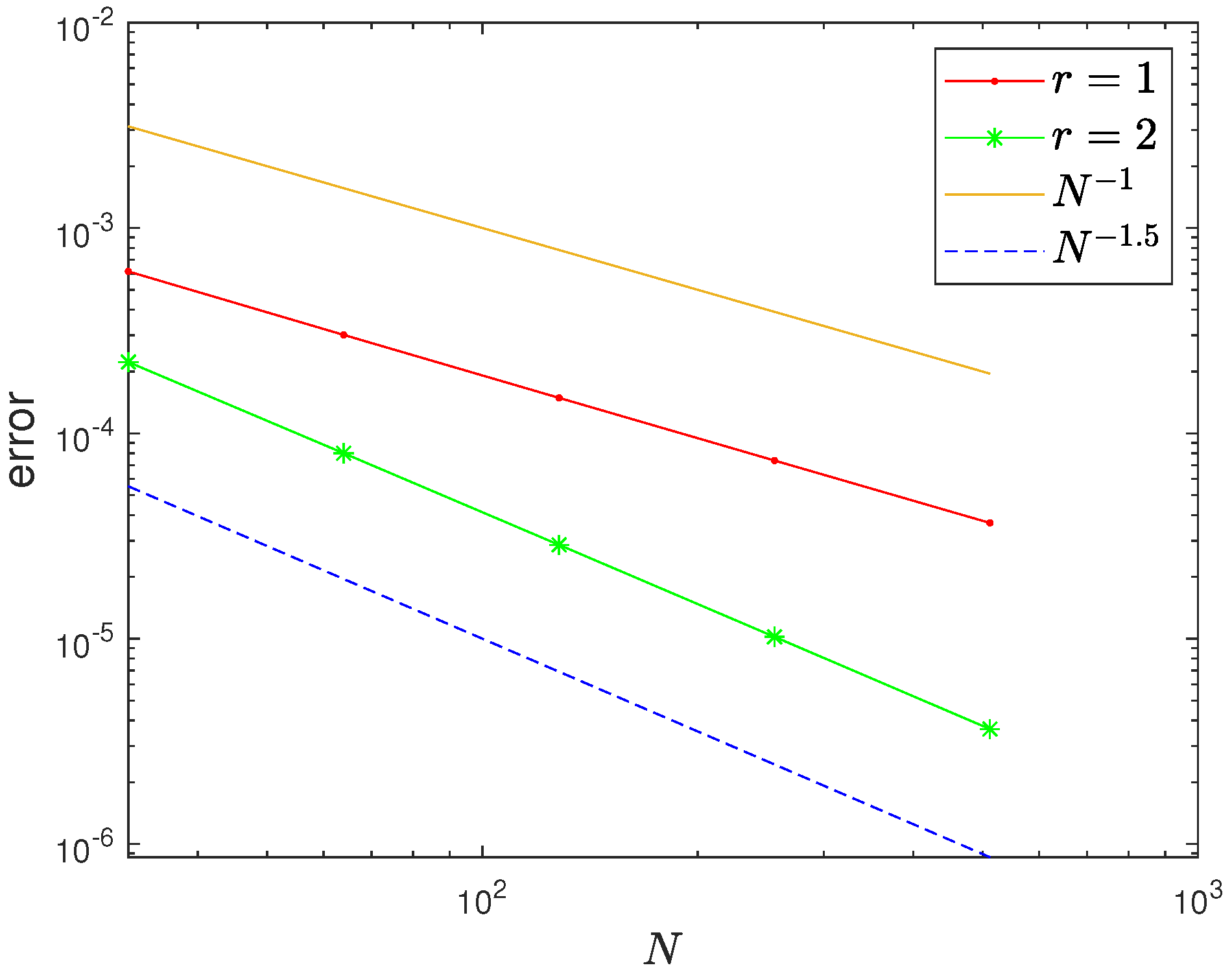
presents the comparison of the computational cost of the numerical scheme between the case $r=1$ and the case $r=2$, where we take $M=\mathrm{10,000}$ and $N=1000$ to compute the local error of our scheme. From which one can see that the CPU times are comparable between the uniform mesh $(r=1)$ and graded mesh $(r=2)$, but the latter attains higher convergence rates. Figure 1 shows the convergence rates in the case $\alpha =0.5$ for uniform mesh $(r=1)$ and graded mesh $(r=2)$, and it is clear that the case $r=2$ has a higher convergence rate.

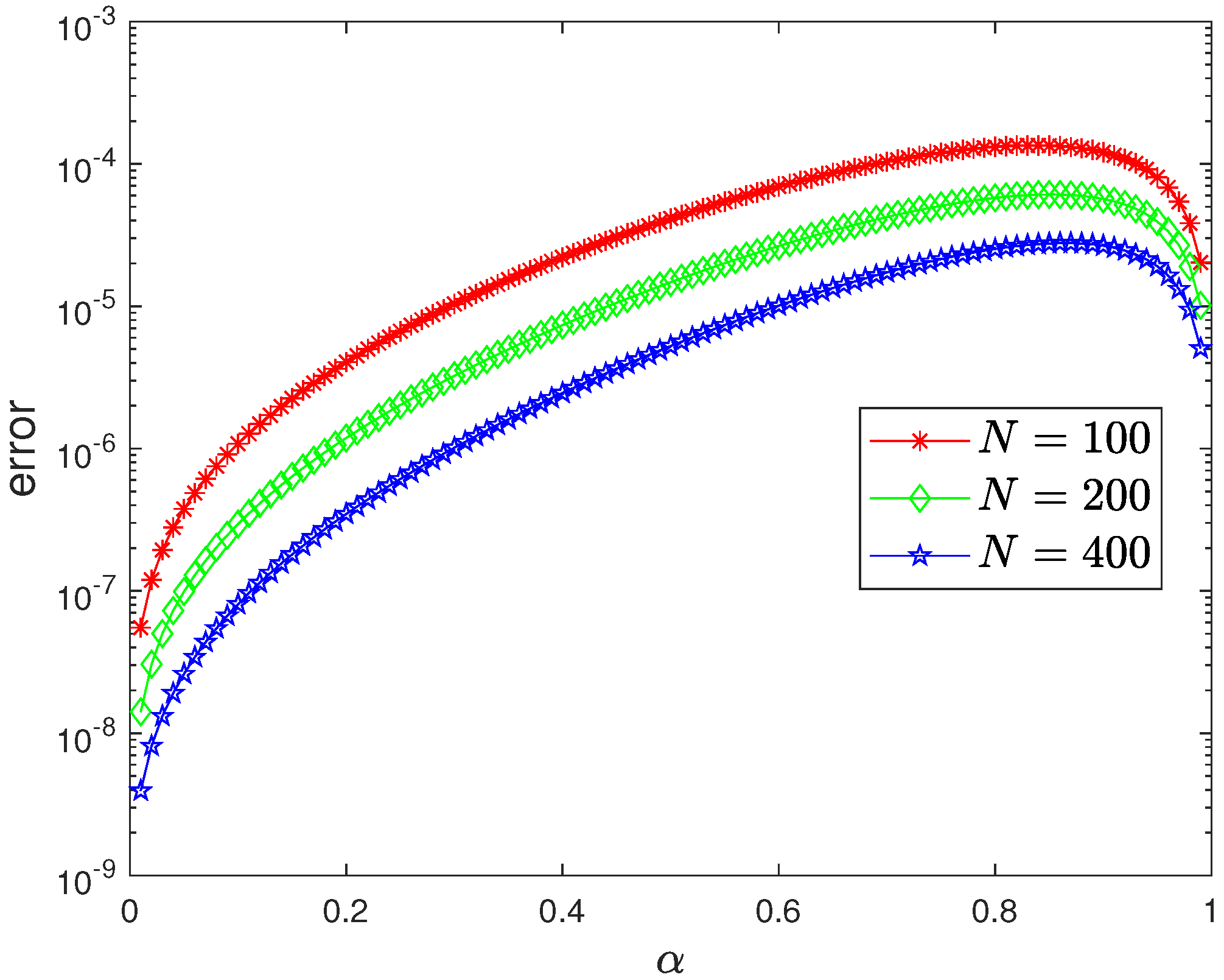
In Table 4, it is interesting to see that the local errors increase as $\alpha$ increases, so we test the local errors for various $\alpha$ between $(0,1)$, and the results are presented in Figure 2. From this figure, we can see that the errors increase when $\alpha$ increases (this is natural as the convergence rates worsen as $\alpha$ increases), but when $\alpha$ approaches $1^{-}$, the errors then decrease (at present we do not know why).

Example 2.

Let $\Omega =(0,1)$, $T=1$, $a=1/32$, $b=0.05-a$, $c=0.05$, the function $f=0$, the initial condition $\varphi \left(x\right)=sin\left(x\right)$.

Since the exact solution to Example 2 is unknown, we use the two-mesh principle in [28] to estimate the convergence rates of our computed solutions. The local differences $D_L^N$ of the two-mesh are defined by the following:

$$\begin{array}{c}\hfill D_L^N={\parallel u^N-w^{2N}\parallel }_{\infty },\end{array}$$

where $w_i^n$ with $0\le n\le 2N$ is computed on a second temporal mesh $t_n=T{(n/2N)}^r$ with the same mesh of $u_i^n$ in space. The estimate convergence rates are computed by the following:

$${log}_2({\displaystyle \frac{D_L^N}{D_L^{2N}}}).$$

We also take $M=10,000$ to eliminate the contamination of the spatial errors.

Table 8. Local differences $D_L^N$ and orders of convergence for Example 2 when $r=1$.

N	$\mathit{\alpha }=0.3$			$\mathit{\alpha }=0.5$			$\mathit{\alpha }=0.7$
	${\mathit{D}}_{\mathit{L}}^{\mathit{N}}$	$\mathit{order}$		${\mathit{D}}_{\mathit{L}}^{\mathit{N}}$	$\mathit{order}$		${\mathit{D}}_{\mathit{L}}^{\mathit{N}}$	$\mathbf{order}$
10	1.4425e-03			2.6619e-03			4.1485e-03
20	6.8909e-04	1.0658		1.2611e-03	1.0778		1.9866e-03	1.0623
40	3.3586e-04	1.0368		6.0918e-04	1.0498		9.6206e-04	1.0461
80	1.6547e-04	1.0213		2.9770e-04	1.0330		4.6948e-04	1.0351
160	8.2023e-05	1.0125		1.4655e-04	1.0225		2.3033e-04	1.0274

,

Table 9. Local differences $D_L^N$ and orders of convergence for Example 2 when $r=2$.

N	$\mathit{\alpha }=0.3$			$\mathit{\alpha }=0.5$			$\mathit{\alpha }=0.7$
	${\mathit{D}}_{\mathit{L}}^{\mathit{N}}$	$\mathit{order}$		${\mathit{D}}_{\mathit{L}}^{\mathit{N}}$	$\mathit{order}$		${\mathit{D}}_{\mathit{L}}^{\mathit{N}}$	$\mathit{order}$
10	5.8830e-04			1.7907e-03			3.9057e-03
20	1.8369e-04	1.6793		6.4328e-04	1.4770		1.6191e-03	1.2704
40	5.7613e-05	1.6728		2.3082e-04	1.4787		6.6566e-04	1.2823
80	1.8052e-05	1.6742		8.2593e-05	1.4827		2.7247e-04	1.2887
160	5.6425e-06	1.6778		2.9469e-05	1.4868		1.1122e-04	1.2927

and

Table 10. Local differences $D_L^N$ and orders of convergence for Example 2 when $r=(2-\alpha )/\alpha$.

N	$\mathit{\alpha }=0.3$			$\mathit{\alpha }=0.5$			$\mathit{\alpha }=0.7$
	${\mathit{D}}_{\mathit{L}}^{\mathit{N}}$	$\mathit{order}$		${\mathit{D}}_{\mathit{L}}^{\mathit{N}}$	$\mathit{order}$		${\mathit{D}}_{\mathit{L}}^{\mathit{N}}$	$\mathit{order}$
10	1.1832e-03			2.1661e-03			3.8024e-03
20	3.7893e-04	1.6427		7.6708e-04	1.4977		1 1.5835e-03	1.2638
40	1.2181e-04	1.6373		2.7211e-04	1.4952		6.5428e-04	1.2751
80	3.9009e-05	1.6428		9.6643e-05	1.4935		2.6902e-04	1.2822
160	1.2456e-05	1.6470		3.4325e-05	1.4934		1.1022e-04	1.2873

present the two-mesh differences and convergence orders for Example 2 with difference choice of r, which agrees with our theoretical prediction, i.e., just choosing $r=2$, the optimal convergence order $2-\alpha$ is obtained.

8. Conclusions

In this work, a fully discrete finite difference scheme for a time-fractional Black-Scholes equation with weakly singular solutions is established, and a pointwise error estimate of the fully discrete scheme is given by using a discrete comparison principle. It should be noted that we used the L1 scheme for the discretization of the time-fractional derivative, which at most attains a $2-\alpha$ convergence rate, so future work may involve how to construct some higher-order schemes and establish their associated stability and convergence.