Real-Time Efficient Approximation of Nonlinear Fractional-Order PDE Systems via Selective Heterogeneous Ensemble Learning

Abstract

Rod-pumping systems represent complex nonlinear systems. Traditional soft-sensing methods used for efficiency prediction in such systems typically rely on complicated fractional-order partial differential equations, severely limiting the real-time capability of efficiency estimation. To address this limitation, we propose an approximate efficiency prediction model for nonlinear fractional-order differential systems based on selective heterogeneous ensemble learning. This method integrates electrical power time-series data with fundamental operational parameters to enhance real-time predictive capability. Initially, we extract critical parameters influencing system efficiency using statistical principles. These primary influencing factors are identified through Pearson correlation coefficients and validated using p-value significance analysis. Subsequently, we introduce three foundational approximate system efficiency models: Convolutional Neural Network-Echo State Network-Bidirectional Long Short-Term Memory (CNN-ESN-BiLSTM), Bidirectional Long Short-Term Memory-Bidirectional Gated Recurrent Unit-Transformer (BiLSTM-BiGRU-Transformer), and Convolutional Neural Network-Echo State Network-Bidirectional Gated Recurrent Unit (CNN-ESN-BiGRU). Finally, to balance diversity among basic approximation models and predictive accuracy, we develop a selective heterogeneous ensemble-based approximate efficiency model for nonlinear fractional-order differential systems. Experimental validation utilizing actual oil-well parameters demonstrates that the proposed approach effectively and accurately predicts the efficiency of rod-pumping systems.

1. Introduction

Crude oil, as a non-renewable resource, plays a vital role in the global energy supply. According to production data [1,2,3,4], artificial lift methods are deployed in over 98% of oil wells worldwide, with rod pumping systems dominating this sector (71% of installations), followed by electrical submersible pumps (14%), gas lift (8%), and other techniques (7%). This distribution makes rod pumping the primary artificial lift method for secondary recovery. Given its prevalence, system efficiency has been widely adopted as a key performance indicator for rod pumping operations. Consequently, the development of robust soft-sensing techniques for real-time efficiency evaluation is critical to optimizing production management and energy consumption.

The pumping unit well system constitutes a complex nonlinear fractional-order partial differential system, typically described using the simplified form of the nonlinear fractional-order partial differential equations as follows:

$$\begin{array}{l}\rho A{\displaystyle \frac{{\partial }^{2}u\left(x,t\right)}{\partial t^2}}={\displaystyle \frac{\partial }{\partial x}}\left(EA{\displaystyle \frac{\partial u\left(x,t\right)}{\partial x}}+EA{\tau }^{\alpha }{\displaystyle \frac{{\partial }^{\alpha }}{\partial t^{\alpha }}}\left({\displaystyle \frac{\partial u\left(x,t\right)}{\partial x}}\right)\right)+f\left(x,t\right)\\ u\left(0,t\right)=0\\ u\left(L,t\right)=A_P\left(p_d-p\right)-A_{rd}{p}_d+\pi L_{p}D\left({\displaystyle \frac{\left(p_d-p\right)\delta }{2L_p}}+{\displaystyle \frac{\mu v_p}{\delta }}{\displaystyle \frac{1}{\sqrt{1-{\epsilon }^2}}}\right)\\ u\left(x,0\right)=0\end{array}$$

(1)

where

$$p=\left\{\begin{array}{ll}{\left({\displaystyle \frac{V_{og}}{V_{og}+V_x}}\right)}^n\left(p_d+\Delta p_d\right)& ,v_p>0,{\mu }_p\le {\mu }_{pd}\\ p_d+\Delta p_d& ,v_p>0,{\mu }_p\ge {\mu }_{pd}\\ {\left({\displaystyle \frac{V_g}{V_g-\left(V_p-V_x\right)}}\right)}^n\left(p_s-\Delta p_s\right)& ,v_p<0,{\mu }_p\ge {\mu }_{pd}\\ p_s-\Delta p_s& ,v_p<0,{\mu }_p\le {\mu }_{pd}\end{array}\right.$$

(2)

In this model, the fractional derivative operator ${\displaystyle \frac{{\partial }^{\alpha }}{\partial t^{\alpha }}}$ is defined in the Caputo sense, which for a function $g\left(t\right)$ is given by:

$${\displaystyle \frac{{\partial }^{\alpha }g\left(t\right)}{\partial t^{\alpha }}}={\displaystyle \frac{1}{\Gamma \left(n-\alpha \right)}}{\displaystyle {\int }_0^t\frac{g^{\left(n\right)}\left(\tau \right)}{{\left(t-\tau \right)}^{\alpha +1-n}}}d\tau , for n-1<\alpha \le n$$

(3)

where $\rho$ is the density of the sucker rod. $A$ is the cross-sectional area. $u\left(x,t\right)$ is the displacement. $t$ is the time. $x$ is the depth. $E$ is the elastic modulus. $\alpha$ is the fractional order, $0<\alpha \le 1$. $f\left(x,t\right)$ is the external force. $L$ is the length of the sucker rod. $\Gamma \left(\cdot \right)$ is the Gamma function, and $n\in N$. In the context of this model, since $0<\alpha \le 1$, we take $n=1$. $v_p$ is the speed of the sucker rod. ${\mu }_p$ is the displacement of the sucker rod. $p_d$ is discharge pressure. $p_s$ is the submergence pressure. $\Delta p_d$ is the differential pressure across the swing valve. $\Delta p_s$ is that the fixed valve pressure differential has been exceeded. $A_P$ is the cross-sectional area of the piston. $A_{rd}$ is the cross-sectional area of the final sucker rod section. $L_p$ is the plunger length. $\delta$ is the plunger clearance. $\mu$ is viscosity. $V_x$ is the volume of the pump at any given position. $V_{og}$ is the volume of gas in the residual volume when the plunger reaches the bottom dead center. $V_g$ is the volume of gas in the pump barrel at the end of the plunger up stroke.

Current approximate models for rod-pumping system efficiency primarily fall into two categories: mathematical approaches based on nonlinear fractional-order partial differential equations and data-driven models leveraging historical data. While mathematical approaches provide valuable insights into the dynamics of rod pumping systems, they also have several inherent limitations. First, these methods require comprehensive prior datasets and involve intricate mathematical formulations. Second, they demonstrate limited capability in handling the system’s inherent nonlinear dynamics and time-varying characteristics. Finally, the substantial computational overhead of these models severely constrains their real-time prediction performance and adaptive control capabilities. For data-driven approaches based on historical data, their effectiveness heavily relies on high-quality datasets while exhibiting inherent limitations in physical interpretability. This significantly restricts parameter optimization and practical engineering applications. The capability of electrical power time-series acquisition devices to measure power consumption at arbitrary sampling intervals enables real-time prediction of rod pumping system efficiency. However, the exclusive use of time-series data proves insufficient for accurate efficiency estimation, necessitating the integration of electrical power measurements with fundamental system parameters. Furthermore, while existing single-model approaches demonstrate inadequate noise immunity and limited prediction accuracy, conventional ensemble learning methods often fail to properly optimize the trade-off between base learner diversity and prediction accuracy. This highlights the critical need to investigate the impact of ensemble learning strategies that explicitly address this balance on the performance of soft sensing methodologies for rod pumping system efficiency.

To address these challenges, we propose a selective heterogeneous ensemble-based efficiency approximation model for nonlinear fractional-order differential systems. This method first employs statistical principles and one-hot encoding to extract features from time series, spatial sequences, and string-type data. Subsequently, primary features are identified through Pearson correlation analysis and statistical significance testing. Following this, we develop three fundamental approximation models: CNN-ESN-BiLSTM, BiLSTM-BiGRU-Transformer, and CNN-ESN-BiGRU. Additionally, we introduce two enhanced optimization algorithms: a multi-strategy integrated multi-objective Mantis Search Algorithm (MSA) and a multi-strategy integrated Hippopotamus Optimization Algorithm (HOA). Finally, we establish the proposed selective heterogeneous ensemble-based efficiency approximation model tailored for nonlinear fractional-order differential systems. The specific contributions of this paper are:

(1)

Feature extraction is performed on time-series data, spatial-sequence data, and string-type data using statistical principles and one-hot encoding, with subsequent identification of dominant features through Pearson correlation analysis and statistical significance testing.

(2)

Three fundamental approximation models have been developed: a CNN-ESN-BiLSTM architecture, a BiLSTM-BiGRU-Transformer framework, and a CNN-ESN-BiGRU network, with comprehensive experimental validation including both full implementation and ablation studies.

(3)

A multi-strategy enhanced multi-objective mantis search algorithm and a multi-strategy improved hippopotamus optimization algorithm are developed, with their precision validated through benchmark test functions.

(4)

A selective heterogeneous ensemble-based efficiency approximation model for nonlinear fractional-order partial differential equation (FPDE) systems was proposed by integrating the enhanced optimization algorithms with three base models while systematically balancing the diversity of base learners and prediction accuracy. Comprehensive experimental validation was then performed, including full-implementation tests and ablation studies.

2. Related Work

2.1. Approximate Models Based on Nonlinear Fractional-Order Partial Differential Equations

Current approximation models for rod pumping system efficiency primarily utilize mathematical frameworks based on rod string longitudinal vibration, initially established by Gibbs in 1963 [5]. Subsequent research has refined vibration modeling through diverse approaches: Langbauer investigated rod string dynamics via finite element analysis [6], while Lukasiewicz examined longitudinal vibrations in deviated wells [7]. Wang analyzed gas–liquid separation effects on vibration [8], and Xing derived an improved simulation model incorporating nonlinear plunger loads and rod friction [9,10]. Li introduced equivalent resistance coefficients based on friction loss equivalence [11], Moreno explored deviated-well vibration behavior [12], and Wang developed a simplified thermoelastic longitudinal vibration model [13]. Yin established analytical solutions for longitudinal vibration [14], whereas Dong created a simulation model accounting for real-time power frequency variations and motor torque transients [15]. Wang formulated a nonlinear coupled lateral vibration model for deviated wells [16], Lekia established rod-fluid coupled vibration equations [17], Dale proposed enhanced longitudinal vibration models with novel boundary conditions [18], and Ma developed multiphase-flow-based vibration equations with efficiency prediction models [19]. Despite significant advances, these models typically rely on simplifying assumptions and require complex mathematical formulations, exhibiting limited capability to address inherent nonlinear dynamics and time-varying characteristics. Consequently, they are generally unsuitable for real-time rod-pump efficiency prediction.

2.2. Data-Driven Approximate Models Based on Historical Data Mining

With the advancement of computational technologies, researchers have developed diverse soft-sensing methods through data mining. Leng [20] proposed a dynamic fluid-level soft-sensing technique for rod-pump systems. Bai et al. [21] established a method for predicting oil saturation-pressure relationships along tight condensate gas well flow paths and developed a transient multiphase production prediction model. Wang [22] formulated a drift-flux model to forecast phase-specific superficial velocities. Yang [23] employed a gated recurrent network for production prediction. Qu [24] created a vibration-state classification soft sensor using deep and machine learning fusion. Zhang [25] introduced a physics-constrained machine learning approach for direct pore pressure prediction from seismic data. Rene et al. [26] proposed a flow soft-sensing method for IoT devices in near-periodic applications. Novel deep learning-based soft-sensor techniques have also emerged [27,28,29,30]. Regarding rod-pump efficiency, Lu [31] developed a system efficiency feature analysis method, while Tan and Ma [32,33,34] proposed a historical data-driven soft-sensing approach. However, these existing data-driven methods for rod-pump efficiency prediction lack real-time applicability, rendering them unsuitable for online estimation.

2.3. Ensemble Learning

Ensemble learning demonstrates significant potential for performance enhancement and finds widespread application across diverse domains. Conventional ensemble techniques typically use empirical approaches for base learner selection. Recent advances include Tan et al.’s LSTM-based hybrid ensemble prediction model [35], Huang et al.’s random walk-based clustering similarity ensemble [36], and Tang et al.’s residual learning-enhanced error estimation method [37]. The Stacking framework has been extensively applied to prediction tasks [38,39,40,41], while Guo et al. developed a multi-classifier CNN ensemble architecture [42]. Notable contributions also encompass Nai et al.’s historical snapshot-based visual tracker [43], Li et al.’s classification-regression ensemble localization system [44], and Peng et al.’s deep reinforcement learning ensemble for flatness control [45]. Since empirical base-learner selection introduces substantial human bias, researchers have begun exploring selective ensemble techniques [46,47,48]. Although initial work on selective homogeneous ensembles shows promise, this approach can lead to a reduction in base-learner diversity due to the selection of performant but similar models.

3. Methodology

3.1. Multi-Strategy Integrated Mantis Search Multi-Objective Algorithm

The traditional Mantis Search multi-objective optimization algorithm [49] suffers from low precision, weak global search capability, and susceptibility to local optima convergence. To address these limitations, we propose a multi-strategy integrated model (MS-MOSA). The core components of this enhanced algorithm are as follows:

Strategy 1: To enhance population diversity, we employ a population initialization method that combines Latin hypercube sampling, which ensures uniform coverage of the search space, with sine-based chaotic initialization, which introduces nonlinear perturbations to escape local optima. The mathematical model is given as follows:

$$X=LHS\left(N,d\right)\subset {\left[0,1\right]}^{N\times d}$$

(4)

$$X^{\prime }={\displaystyle \frac{\sin \left(2\pi X\right)+1}{2}}$$

(5)

$$x=a+X^{\prime }\left(b-a\right)$$

(6)

where $LHS\left(\cdot \right)$ is Latin hypercube initialization, $N$ is the total number of samples. $d$ is the dimensionality. $a$ is the lower bound. $b$ is the upper bound.

Strategy 2: To enhance the ambush predator’s nonlinear search capability, enabling it to escape local optima and locate more comprehensive global solutions, we developed a mathematical model of ambush predator behavior characterized by a nonlinear distance factor. This factor dynamically adjusts search step sizes, enhancing global exploration in early iterations and local exploitation in later phases. The nonlinear distance factor increases the ambush predator’s dynamic range, further influencing mantis search behavior by promoting more aggressive movement when prey is distant and finer movements when prey is near. The proposed nonlinear ambusher behavior model is as follows:

$$X_i\left(t+1\right)=X_i\left(t\right)+\alpha \cdot \left(X_{ar}\left(t\right)-X_a\left(t\right)\right)$$

(7)

$$\alpha =\cos \left(\pi r_6\right)\cdot \mu$$

(8)

$$\mu =1-{\displaystyle \frac{1}{e-1}}\times \left(e^{{\displaystyle \frac{t}{T}}}-1\right)$$

(9)

where $X_{ar}\left(t\right)$ is the global optimum. $\alpha$ is a parameter controlling the position of the mantis’ head. $r_6$ is a value randomly selected within the interval [0, 1]. $\mu$ is the nonlinear distance factor. $T$ is the maximum number of generations.

Strategy 3: In their natural environment, prey species forage actively and may inadvertently venture within a mantis’s striking distance. To improve global search performance, we model prey escape dynamics using a nonlinear strategy. This approach enhances the optimizer’s ability to escape local optima by promoting broader exploration across the search space. Consequently, these nonlinear reactions modulate the mantis’s search behavior: they adaptively control movement intensity—favoring larger strides when prey is far and finer adjustments when prey is close—thereby improving the balance between exploration and exploitation. The specific formula is as follows:

$$X_i\left(t+1\right)=X_{ar}\left(t\right)+\left(r_7\times 2-1\right)\times \left(1-{\displaystyle \frac{1}{e-1}}\times \left(e^{{\displaystyle \frac{t}{T}}}-1\right)\right)\times \left(r_8 · \left(X^{up}-X^{low}\right)+X^{low}\right)$$

(10)

Strategy 4: To enhance global search capability and convergence performance, we integrate the sparrow search algorithm with mantis mating behavior, which collectively improves the accuracy and efficiency of the optimization process. The refined male attraction model is:

$$x_i\left(t+1\right)=\left\{\begin{array}{l}Q\times \exp \left({\displaystyle \frac{X^b-x_i\left(t\right)}{i^2}}\right), i>{\displaystyle \frac{N}{2}}\\ X^b+\left|x_i\left(t\right)-X^b\right|\times A^{+}\times L, i\le {\displaystyle \frac{N}{2}}\end{array}\right.$$

(11)

where $X^b$ is the current global optimal position.

Strategy 5: To improve global search and convergence, we integrate the sparrow optimization strategy with mantis mating behavior, enhancing accuracy. This hybridization leverages the exploratory strength of sparrow foraging and the exploitative precision of mating rituals, allowing the algorithm to navigate complex search spaces more effectively and avoid premature convergence. The refined male attraction model is:

$$X_i\left(t+1\right)=\left(X_i\left(t\right)\ast U+X_a\ast \left(1-U\right)\right)\ast \left(w\ast {\displaystyle \frac{1}{\pi \mathrm{Ƴ}\left[1+{\left(\frac{x-x_0}{\mathrm{Ƴ}}\right)}^2\right]}}+w\ast {\displaystyle \frac{1}{\sigma \sqrt{2\pi }}}{e}^{-{\displaystyle \frac{1}{2}}{\left({\displaystyle \frac{x-\mu }{\sigma }}\right)}^2}\right)$$

(12)

$$X_a=X_{11}\left(t\right)+r_{18}\ast \left(-X_{11}\left(t\right)+X_i\left(t\right)\right)$$

(13)

$$w=\left(w_{z1}+w_{z2}+w_{z3}+w_{z4}\right)\times \cos \left({\displaystyle \frac{\pi }{2}}{\displaystyle \frac{t}{T_{\max }}}\right)$$

(14)

$$w_{z1}=-{\displaystyle \frac{\left(t-T_1\right)\times \left(t-T_2\right)\times \left(t-T_{\max }\right)}{T_1\times T_2\times T_{\max }}}\times w_{star}$$

(15)

$$w_{z2}={\displaystyle \frac{t\times \left(t-T_2\right)\times \left(t-T_{\max }\right)}{T_1\times \left(T_1-T_2\right)\times \left(T_1-T_{\max }\right)}}\times w_1$$

(16)

$$w_{z3}={\displaystyle \frac{t\times \left(t-T_1\right)\times \left(t-T_{\max }\right)}{T_2\times \left(T_2-T_1\right)\times \left(T_2-T_3\right)}}\times w_2$$

(17)

$$w_{z4}={\displaystyle \frac{t\times \left(t-T_1\right)\times \left(t-T_2\right)}{T_{\max }\times \left(T_{\max }-T_1\right)\times \left(T_{\max }-T_2\right)}}\times w_{end}$$

(18)

where ${\sigma }^2$ is the variance. $\mu$ is the mean. $\mathrm{Ƴ}$ is the scale parameter. $r_{18}$ is a vector randomly generated within the range [0, 1]. $T_{\max }$ is the maximum number of iterations. $t$ refers to any given iteration step. $X_{11}\left(t\right)$ is the value of the first dimension of the first mantis. $T_1$, $T_2$, and $T_3$ are random numbers within the interval $[0,T_{\max }]$, with $T_1<T_2<T_3$ as a condition. $w_{star}$, $w_1$, $w_2$ and $w_{end}$ are random numbers within the range [0, 1].

Strategy 6: Inspired by the adaptive behavior of female mantises consuming males after mating, we propose a mathematical model designed to enhance the search for the global optimum and facilitate rapid escape from local optima, thereby reducing errors. The model incorporates an adaptive nonlinear Newton–sine weight coefficient that dynamically balances exploration and exploitation through Newton-based sine modulation. Additionally, a golden sine function—embedding the golden ratio within a sinusoidal transformation—is introduced to steer the search trajectory toward more promising regions. The corresponding calculation formula is given as follows:

$$X_i\left(t+1\right)=\left(1-w\right)\times X_i\left(t\right)\times \left|\sin \left(r_1\right)\right|-w\times r_2\times \sin \left(r_1\right)\times \left|c_1\times X^b-c_2\times X_i\left(t\right)\right|$$

(19)

$$w=1-\left(w_{nstar}+w_{z11}+w_{z21}+w_{z51}\right)\times \left(1-\sin \left({\displaystyle \frac{\pi }{2}}{\displaystyle \frac{t}{T_{\max }}}\right)\right)$$

(20)

$$w_{z11}=\left({\displaystyle \frac{w_{11}-w_{nstar}}{T_{11}}}\right)\times t$$

(21)

$$w_{z21}=\left\{{\displaystyle \frac{w_{22}-w_{nstar}-\left(\frac{w_{11}-w_{nstar}}{T_{11}}\right)\times T_{22}}{T_{22}\times \left(T_{22}-T_{11}\right)}}\right\}\times t\times \left(t-T_{11}\right)$$

(22)

$$w_{z31}=\left({\displaystyle \frac{w_{11}-w_{nstar}}{T_{11}}}\right)\times T_{\max }$$

(23)

$$w_{z41}=\left({\displaystyle \frac{w_{22}-w_{nstar}-\left(\frac{w_{11}-w_{nstar}}{T_{11}}\right)\times T_{22}}{T_{22}\times \left(T_{22}-T_{11}\right)}}\right)\times T_{\max }\times \left(T_{\max }-T_{11}\right)$$

(24)

$$w_{z51}=\left({\displaystyle \frac{w_{nend}-w_{nstar}-w_{z31}-w_{z41}}{T_{\max }\times \left(T_{\max }-T_{11}\right)\times \left(T_{\max }-T_{22}\right)}}\right)\times t\times \left(t-T_{11}\right)\times \left(t-T_{22}\right)$$

(25)

where $T_{11}$ and $T_{22}$ are random numbers between $\left[0,T_{\max }\right]$. $w_{11}$ and $w_{22}$ are random numbers between $\left[w_{nstar},w_{nend}\right]$. $w_{nstar}=1.25$, $w_{nend}=0$, $T_{11}={\displaystyle \frac{T_{\max }}{10}}$, and $T_2={\displaystyle \frac{T_{\max }}{5}}$.

3.2. Multi-Strategy Integrated Hippo Optimization Algorithm

The traditional Hippopotamus Optimization Algorithm (HOA) [50] suffers from low search precision, inadequate global search capability, and a susceptibility to local optima entrapment. To address these limitations, we propose a multi-strategy integrated model. The core mechanisms of this enhanced algorithm are detailed as follows:

Strategy 1: Latin Hypercube, Sine Initialization and Cubic Initialization Mixed Initialization.

To enhance population initialization diversity, we propose a hybrid sequential initialization combining Latin hypercube sampling, sine-based chaotic initialization, and cubic initialization. Latin hypercube sampling ensures uniform coverage of the search space, sine-based chaotic initialization introduces nonlinear dynamics to escape local optima, and cubic initialization further refines local search precision. Its formula is:

$$X=LHS\left(N,d\right)\subset {\left[0,1\right]}^{N\times d}$$

(26)

$$S_{i,j}={\displaystyle \frac{\sin \left(2\pi X_{i,j}\right)+1}{2}}, S_{i,j}\in \left[0,1\right]$$

(27)

$$H_{i,j}={\left({\displaystyle \frac{\sin \left(2\pi S_{i,j}\right)+1}{2}}\right)}^3, H_{i,j}\in \left[0,1\right]$$

(28)

where $LHS\left(\cdot \right)$ is Latin hypercube initialization. $N$ is the total number of samples. $d$ is the dimensionality.

Strategy 2: To simulate the hippo’s escape behavior from predators, we incorporate a triangular walking movement pattern. This strategy enhances the randomness and unpredictability of movement trajectories, allowing the algorithm to explore a broader search space and avoid premature convergence.

First, the distance $L_1$ between the hippo and the predator is determined. Then, the range of the hippo’s step length $L_2$ is obtained. The formula for the triangular walking strategy is as follows:

$$\begin{array}{l}{L}_1=X_b\left(t\right)-X_c\left(t\right)\\ L_2=rand()\times L_1\end{array}$$

(29)

where $L_1$ is the distance between the hippo. $L_2$ is the range of the hippo’s step length. $X_b\left(t\right)$ is the position of the hippo. $X_c\left(t\right)$ is the position of the predator, and $rand()$ is a randomly generated number within the range $[0,1]$.

The walking direction $\beta$ is further defined as:

$$\beta =2\times \pi \times rand()$$

(30)

where $\beta$ represents the walking direction.

Finally, the formula for calculating the hippo’s position after walking is:

$$P={L^2}_1+{L^2}_2-2\times L_1\times L_2\times \cos \left(\beta \right)$$

(31)

$$X_b\left(t+1\right)=X_b\left(t\right)+r\times P$$

(32)

where $X_b\left(t+1\right)$ represents the position of the hippo after walking.

Strategy 3: To mitigate the challenges of strong parameter dependency and high computational complexity associated with the triangular walking strategy, we incorporated the golden sine algorithm. This integration utilizes the properties of the golden ratio and sine function to enhance the efficiency of the triangular walking strategy. The position update formula, refined by incorporating the golden sine algorithm, is as follows:

$${X^{t+1}}_i={X^t}_i\cdot \left|\sin \left(r_1\right)\right|-r_2\cdot \sin \left(r_1\right)\cdot \left|x_1\cdot {D^t}_i-x_2\cdot {X^t}_i\right|$$

(33)

where

$$x_1=a\cdot \left(1-{\displaystyle \frac{\sqrt{5}-1}{2}}\right)+b\cdot \left({\displaystyle \frac{\sqrt{5}-1}{2}}\right)$$

(34)

$$x_2=a\cdot \left({\displaystyle \frac{\sqrt{5}-1}{2}}\right)+b\cdot \left(1-\left({\displaystyle \frac{\sqrt{5}-1}{2}}\right)\right)$$

(35)

where $a,b$ represents the initial value for the golden ratio search, while $a=-\pi$ and $b=\pi$ refer to additional parameters.

3.3. CNN–ESN–BiLSTM–Based Online Approximate Models for Rod-Pump System Efficiency

Traditional data-mining models for estimating the efficiency of rod-pumping systems have primarily relied on historical data. While useful, these approaches are often limited by concept drift, data bias, latency, and interpretability issues, as they only learn from past observations. Recent advances in sensor technology have enabled the collection of real-time electrical power data, providing a stronger basis for online efficiency approximation. However, using power time-series data alone is still inadequate for accurate predictions. To overcome these challenges, we propose an online efficiency approximation model based on a CNN–ESN–BiLSTM architecture (named CEBS). The model consists of three core modules: feature extraction, feature selection, and real-time approximation. The overall structure is shown in Figure 1.

• Step 1. Feature extraction of spatial sequence data:

Spatial sequence data often consist of a limited number of sampling points, yet exhibit strong sequential dependencies and global structural patterns. Using raw sequences directly can introduce challenges such as high dimensionality, noise, and redundancy, which may impede effective model training. In contrast, statistical descriptors can reduce dimensionality while preserving critical trajectory characteristics—including overall trends, fluctuation ranges, stability, and distribution shapes. To achieve this, we employ four statistical measures—mean, range, variance, and skewness—to extract informative features from the spatial sequences $X_s$. The unified mathematical formulation for spatial feature extraction is expressed as follows:

$$X_{s\mu }={\displaystyle \frac{1}{N}}{\displaystyle \sum _{i=1}^N{X}_s}$$

(36)

$$X_{sR}=\underset{1\le i\le N}{\max }{X}_s-\underset{1\le i\le N}{\min }{X}_s$$

(37)

$$X_{s\sigma }={\displaystyle \frac{1}{N-1}}{\displaystyle \sum _{i=1}^N{\left(X_s-X_{s\mu }\right)}^2}$$

(38)

$$X_{s\gamma }={\displaystyle \frac{\frac{1}{N}{\displaystyle \sum _{i=1}^N{\left(X_s-X_{s\mu }\right)}^3}}{{\left(\frac{1}{N}{\displaystyle \sum _{i=1}^N{\left(X_s-X_{s\mu }\right)}^2}\right)}^{3/2}}}$$

(39)

where $X_{s\mu }$ is the mean of each spatial-sequence data instance. $X_{sR}$ is the range of each spatial-sequence data instance. $X_{s\sigma }$ is the variance of each spatial-sequence data instance, $X_{s\gamma }$ is the skewness of each spatial-sequence data instance, and $N$ is the total number of spatial sequences.

• Step 2. Feature extraction of time series data:

Time-series data $X_t$ often exhibit strong non-stationarity, high dimensionality, and significant noise. In comparison, statistical methods offer an effective way to reduce dimensionality, improve robustness, and capture both global trends and local patterns. Accordingly, nine statistical descriptors—mean, variance, skewness, kurtosis, range, interquartile range, zero-crossing rate, peak count, and power waveform factor—are used to extract representative features from the time-series data. The unified mathematical formulation for this feature extraction process is given as follows:

$$\begin{array}{l}{X}_{t\mu }={\displaystyle \frac{1}{M}}{\displaystyle \sum _{i=1}^M{X}_t},\\ X_{t\sigma }={\displaystyle \frac{1}{M-1}}{\displaystyle \sum _{i=1}^M}{{\displaystyle \left(X_t-X_{t\mu }\right)}}^2\end{array}$$

(40)

$$X_{t\gamma }={\displaystyle \frac{\frac{1}{M}{\displaystyle \sum _{i=1}^M{\left(X_t-X_{t\mu }\right)}^3}}{{\left(\frac{1}{M}{\displaystyle \sum _{i=1}^M{\left(X_t-X_{t\mu }\right)}^2}\right)}^{3/2}}}$$

(41)

$$X_{t\gamma P}={\displaystyle \frac{\frac{1}{M}{\displaystyle \sum _{i=1}^M{\left(X_t-X_{t\mu }\right)}^4}}{{\left(\frac{1}{M}{\displaystyle \sum _{i=1}^M{\left(X_t-X_{t\mu }\right)}^2}\right)}^2}}-3$$

(42)

$$X_{tR}=\underset{1\le i\le M}{\max }{X}_t-\underset{1\le i\le M}{\min }{X}_t$$

(43)

$$X_{tIQ}=X_{t-Q3}-X_{t-Q1}$$

(44)

$$X_{tZC}={\displaystyle \frac{1}{M-1}}{\displaystyle \sum _{i=1}^{M-1}{\rm I}\left(X_{t-i}\cdot X_{t-i+1}<0\right)}$$

(45)

$$X_{t\mathrm{P}e}={\displaystyle \sum _{i=2}^{M-1}{\rm I}\left(X_{t-i-1}<X_{t-i}>X_{t-i+1}\right)}$$

(46)

$$X_{tWFP}={\displaystyle \frac{\sqrt{\frac{1}{M}{\displaystyle \sum _{i=1}^N{X_t}^2}}}{\frac{1}{M}{\displaystyle \sum _{i=1}^N\left|X_t\right|}}}$$

(47)

where $X_{t\mu }$ is the mean of the time series. $X_{t\sigma }$ is the variance. $X_{t\gamma }$ is the skewness. $X_{t\gamma P}$ is the kurtosis. $X_{tR}$ is the range. $X_{tIQ}$ is the interquartile range. $X_{tZC}$ is the zero-crossing rate. $X_{t\mathrm{P}e}$ is the peak count. $X_{tWFP}$ is the waveform factor. $M$ is the total number of time series. $X_{t-i-1}$ represents the value of $i-1$. $X_{t-i}$ represents the value of $i$. $X_{t-i+1}$ represents the value of $i+1$. $X_{t-Q3}$ represents the value of $Q3$. $X_{t-Q1}$ represents the value of $Q1$.

• Step 3. Feature extraction of string data:

Since string data often has no inherent numerical size relationship, it needs to be converted into numerical form before it can be input into a deep learning model. Therefore, we use Label encoding to extract features from string data. The mathematical principle behind string data feature extraction is as follows:

$$X_{string-t}=Label\left(X_{string}\right)$$

(48)

where $Label\left(\cdot \right)$ is the string encoding. $X_{string}$ represents string data. $X_{string-t}$ represents the extracted features of the string.

• Step 4. Build a new numerical feature dataset:

We concatenate the features extracted from time-series data, spatial-sequence data, string data, and numerical data to form a new dataset. The mathematical model is given as follows:

$$X_f=Connection\left(\begin{array}{l}{X}_{s\mu },X_{sR},X_{s\sigma },X_{s\gamma },X_{t\mu },X_{t\sigma },\\ X_{t\gamma },X_{t\gamma P},X_{tR},X_{tIQ},X_{tZC},X_{t\mathrm{P}e},\\ X_{tWFP},X_{numeric},X_{string-t}\end{array}\right)$$

(49)

where $Connection\left(\cdot \right)$ is the concatenation function.

• Step 5. Feature selection:

Since the original dataset suffers from issues such as excessive features, data sparsity, and computational complexity, Pearson correlation analysis combined with p-value significance testing is employed for feature selection, yielding the final input feature set $X_{input}$. The mathematical formulation of the feature selection process applied to the extracted sample dataset is expressed as follows:

$${\overline{x}}_f={\displaystyle \frac{1}{n}}{\displaystyle \sum _{i=1}^n{x}_{fi}}, {\overline{y}}_f={\displaystyle \frac{1}{n}}{\displaystyle \sum _{i=1}^n{y}_{fi}}$$

(50)

$$r={\displaystyle \frac{\frac{1}{n-1}{\displaystyle \sum _{i=1}^n\left(x_{fi}-{\overline{x}}_f\right)\left(y_{fi}-{\overline{y}}_f\right)}}{\sqrt{\frac{1}{n-1}{\displaystyle \sum _{i=1}^n{\left(x_{fi}-{\overline{x}}_f\right)}^2}}\sqrt{\frac{1}{n-1}{\displaystyle \sum _{i=1}^n{\left(y_{fi}-{\overline{y}}_f\right)}^2}}}}$$

(51)

$$T={\displaystyle \frac{r\sqrt{n-2}}{\sqrt{1-r^2}}}~t\left(df=n-2\right)$$

(52)

$$p=1-{{\displaystyle {\int }_{-\infty }^T\frac{\Gamma \left(\frac{\mathrm{n}-1}{2}\right)}{\sqrt{v\pi }\Gamma \left(\frac{\mathrm{n}-2}{2}\right)}\left(1+\frac{{\mu }^2}{v}\right)}}^{-\left({\displaystyle \frac{\mathrm{n}-1}{2}}\right)}d\mu$$

(53)

where $x_{fi}$ is the influencing features in the dataset. $y_{fi}$ is the predictive features in the dataset. $n$ is the total number of samples. ${\overline{x}}_f$ is the average value of $x_{fi}$. ${\overline{y}}_f$ is the average value of $y_{fi}$. $\Gamma \left(\cdot \right)$ is Gamma function. $v$ is free movement. $\mu$ is the average value.

• Step 6. Real-time approximation model prediction:

To address the inherent limitations of low prediction accuracy and limited robustness in conventional single-task models, we propose an integrated framework combining a convolutional neural network (CNN), an echo state network (ESN), and a bidirectional long short-term memory network (BiLSTM) to construct a comprehensive CNN–ESN–BiLSTM model for system efficiency approximation. Initially, the CNN is employed to extract localized feature representations from the selected influential input variables. The resulting feature sequences are subsequently fed into the ESN to model temporal dynamics and capture short-term recurrent patterns. Finally, the reservoir states generated by the ESN are processed by the BiLSTM module, which captures bidirectional long-range dependencies and produces the final prediction output. The mathematical formulation of the entire process is given as follows:

$$y=BiSTM\left(ESN\left(CNN\left(x\right)\right)\right)$$

(54)

where $BiLSTM\left(\cdot \right)$ is a BiLSTM. $ESN\left(\cdot \right)$ is a ESN. $CNN\left(\cdot \right)$ is a CNN.

3.4. BiLSTM–BiGRU–Transformer–Based Approximate Models for Rod-Pump System Efficiency

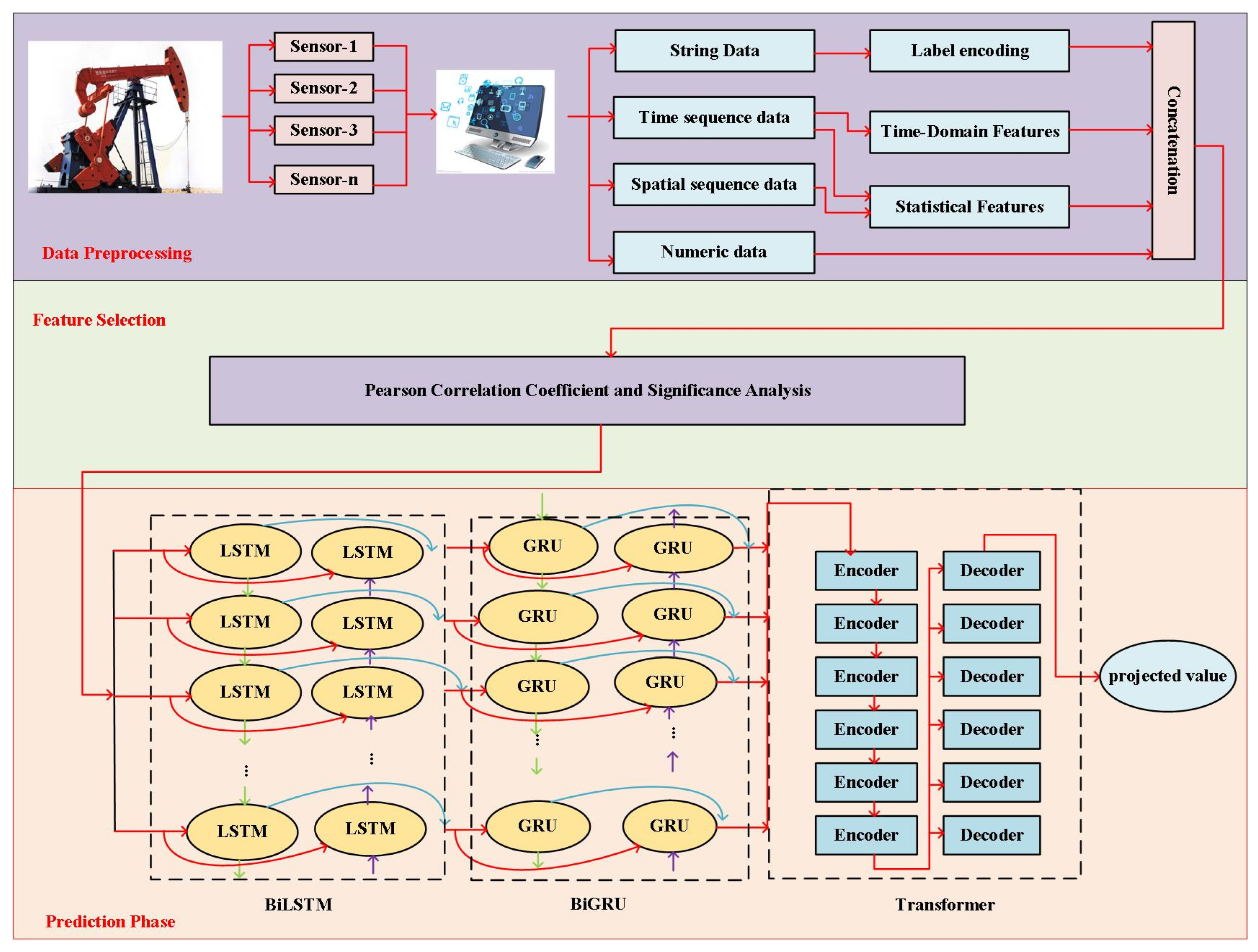
Traditional data-driven models for approximating the efficiency of beam-pumping systems typically rely on historical data. However, such approaches are often susceptible to concept drift, data bias, latency, and issues of interpretability and compliance. To address these challenges, we propose an online efficiency approximation model that integrates BiLSTM, BiGRU, and Transformer—referred to as the BBTS model. The framework consists of three core modules: feature extraction, feature selection, and real-time approximation. The overall architecture is illustrated in Figure 2.

• Step 1. Feature extraction:

To accurately identify features, we apply statistical methods to both spatial and temporal sequence data. For spatial sequences, four statistical descriptors—mean, range, variance, and skewness—are used, as defined in Equations (36)–(39). For temporal sequences, nine descriptors are adopted, including mean, variance, skewness, kurtosis, range, interquartile range, zero-crossing rate, peak count, and power waveform factor, detailed in Equations (40)–(47). For string data, label encoding is applied for feature representation, as specified in Equation (48).

• Step 2. Build a new numerical feature dataset:

We concatenate the features extracted from time-series data, spatial-sequence data, string data, and numerical data to form a new dataset. The mathematical model is given as follows:

$$X_f=Connection\left(\begin{array}{l}{X}_{s\mu },X_{sR},X_{s\sigma },X_{s\gamma },X_{t\mu },X_{t\sigma },\\ X_{t\gamma },X_{t\gamma P},X_{tR},X_{tIQ},X_{tZC},X_{t\mathrm{P}e},\\ X_{tWFP},X_{numeric},X_{string-t}\end{array}\right)$$

(55)

where $Connection\left(\cdot \right)$ is the concatenation function.

• Step 3. Feature selection:

Since the original dataset suffers from issues such as excessive features, data sparsity, and computational complexity, Pearson correlation analysis combined with p-value significance testing is employed for feature selection, yielding the final input feature set $X_{input}$. The mathematical formulation of the feature selection process applied to the extracted sample dataset is expressed as follows:

$${\overline{x}}_f={\displaystyle \frac{1}{n}}{\displaystyle \sum _{i=1}^n{x}_{fi}}, {\overline{y}}_f={\displaystyle \frac{1}{n}}{\displaystyle \sum _{i=1}^n{y}_{fi}}$$

(56)

$$r={\displaystyle \frac{\frac{1}{n-1}{\displaystyle \sum _{i=1}^n\left(x_{fi}-{\overline{x}}_f\right)\left(y_{fi}-{\overline{y}}_f\right)}}{\sqrt{\frac{1}{n-1}{\displaystyle \sum _{i=1}^n{\left(x_{fi}-{\overline{x}}_f\right)}^2}}\sqrt{\frac{1}{n-1}{\displaystyle \sum _{i=1}^n{\left(y_{fi}-{\overline{y}}_f\right)}^2}}}}$$

(57)

$$T={\displaystyle \frac{r\sqrt{n-2}}{\sqrt{1-r^2}}}~t\left(df=n-2\right)$$

(58)

$$p=1-{{\displaystyle {\int }_{-\infty }^T\frac{\Gamma \left(\frac{\mathrm{n}-1}{2}\right)}{\sqrt{v\pi }\Gamma \left(\frac{\mathrm{n}-2}{2}\right)}\left(1+\frac{{\mu }^2}{v}\right)}}^{-\left({\displaystyle \frac{\mathrm{n}-1}{2}}\right)}d\mu$$

(59)

where $x_{fi}$ is the influencing features in the dataset. $y_{fi}$ is the predictive features in the dataset. $n$ is the total number of samples. ${\overline{x}}_f$ is the average value of $x_{fi}$. ${\overline{y}}_f$ is the average value of $y_{fi}$. $\Gamma \left(\cdot \right)$ is Gamma function. $v$ is free movement. $\mu$ is the average value.

• Step 4. Real-time approximation model prediction:

To address the limitations of conventional single-model approaches—such as low prediction accuracy and poor noise robustness—we develop a hybrid model combining BiLSTM, BiGRU, and Transformer. First, the selected features are input to the BiLSTM to capture both long- and short-term dependencies in the sequence. The output from BiLSTM is then processed by the BiGRU for deeper sequential modeling. Finally, the BiGRU output is passed into the Transformer encoder to model global feature interactions and dependencies, producing the final prediction. The overall mathematical formulation of this process is given as follows:

$$h_t^{BiLSTM}=[LST{M}_f\left(x_t,\overrightarrow{h_{t-1}}\right);LST{M}_b\left(x_t,\overleftarrow{h_{t+1}}\right)]$$

(60)

$$h_t^{BiGRU}=[GR{U}_f\left(h_t^{BiLSTM},\overrightarrow{h_{t-1}}\right);GR{U}_b\left(h_t^{BiLSTM},\overleftarrow{h_{t+1}}\right)]$$

(61)

$$y=Transformer\left(h_t^{BiGRU}\right)$$

(62)

where $LST{M}_f\left(\cdot \right)$ is a forward LSTM. $LST{M}_b\left(\cdot \right)$ is a backward LSTM. $GR{U}_f\left(\cdot \right)$ is a forward GRU. $GR{U}_b\left(\cdot \right)$ is a backward GRU. $TransformerEnocder\left(\cdot \right)$ is Transformer.

3.5. CNN-ESN-BiGRU–Based Approximate Models for Rod-Pump System Efficiency

Traditional data-driven soft sensing methods for estimating rod-pumping system efficiency typically rely on historical data. However, these methods are often affected by concept drift, data bias, latency, and challenges related to compliance and interpretability. To overcome these limitations, we propose an online efficiency estimation model that integrates CNN, ESN, and BiGRU (referred to as CEGS). The overall structure of the model is shown in Figure 3.

• Step 1. Feature extraction:

To accurately identify features, we apply statistical methods to both spatial and temporal sequence data. For spatial sequences, four statistical descriptors—mean, range, variance, and skewness—are used, as defined in Equations (36)–(39). For temporal sequences, nine descriptors are adopted, including mean, variance, skewness, kurtosis, range, interquartile range, zero-crossing rate, peak count, and power waveform factor, detailed in Equations (40)–(47). For string data, label encoding is applied for feature representation, as specified in Equation (48).

• Step 2. Build a new numerical feature dataset:

We concatenate the features extracted from time-series data, spatial-sequence data, string data, and numerical data to form a new dataset. The mathematical model is given as follows:

$$X_f=Connection\left(\begin{array}{l}{X}_{s\mu },X_{sR},X_{s\sigma },X_{s\gamma },X_{t\mu },X_{t\sigma },\\ X_{t\gamma },X_{t\gamma P},X_{tR},X_{tIQ},X_{tZC},X_{t\mathrm{P}e},\\ X_{tWFP},X_{numeric},X_{string-t}\end{array}\right)$$

(63)

where $Connection\left(\cdot \right)$ is the concatenation function.

• Step 3. Feature selection:

Since the original dataset suffers from issues such as excessive features, data sparsity, and computational complexity, Pearson correlation analysis combined with p-value significance testing is employed for feature selection, yielding the final input feature set $X_{input}$. The mathematical formulation of the feature selection process applied to the extracted sample dataset is expressed as follows:

$${\overline{x}}_f={\displaystyle \frac{1}{n}}{\displaystyle \sum _{i=1}^n{x}_{fi}}, {\overline{y}}_f={\displaystyle \frac{1}{n}}{\displaystyle \sum _{i=1}^n{y}_{fi}}$$

(64)

$$r={\displaystyle \frac{\frac{1}{n-1}{\displaystyle \sum _{i=1}^n\left(x_{fi}-{\overline{x}}_f\right)\left(y_{fi}-{\overline{y}}_f\right)}}{\sqrt{\frac{1}{n-1}{\displaystyle \sum _{i=1}^n{\left(x_{fi}-{\overline{x}}_f\right)}^2}}\sqrt{\frac{1}{n-1}{\displaystyle \sum _{i=1}^n{\left(y_{fi}-{\overline{y}}_f\right)}^2}}}}$$

(65)

$$T={\displaystyle \frac{r\sqrt{n-2}}{\sqrt{1-r^2}}}~t\left(df=n-2\right)$$

(66)

$$p=1-{{\displaystyle {\int }_{-\infty }^T\frac{\Gamma \left(\frac{\mathrm{n}-1}{2}\right)}{\sqrt{v\pi }\Gamma \left(\frac{\mathrm{n}-2}{2}\right)}\left(1+\frac{{\mu }^2}{v}\right)}}^{-\left({\displaystyle \frac{\mathrm{n}-1}{2}}\right)}d\mu$$

(67)

where $x_{fi}$ is the influencing features in the dataset. $y_{fi}$ is the predictive features in the dataset. $n$ is the total number of samples. ${\overline{x}}_f$ is the average value of $x_{fi}$. ${\overline{y}}_f$ is the average value of $y_{fi}$. $\Gamma \left(\cdot \right)$ is Gamma function. $v$ is free movement. $\mu$ is the average value.

• Step 4. Real-time approximation model prediction:

Conventional single-model approaches often exhibit limited prediction accuracy and insufficient robustness to noise. To overcome these shortcomings, we propose a hybrid CNN–ESN–BiGRU model that integrates convolutional, echo state, and bidirectional recurrent networks. The model operates in three stages: first, the CNN extracts local feature representations from relevant inputs; second, the ESN captures temporal dynamics in the feature sequence; finally, the BiGRU models bidirectional long-term dependencies to generate the final prediction. This multi-stage architecture enhances both representational capacity and robustness in efficiency approximation. The overall mathematical formulation of this process is given as follows:

$$y=BiGRU\left(ESN\left(CNN\left(x\right)\right)\right)$$

(68)

where $BiGRU\left(\cdot \right)$ is a BiGRU. $ESN\left(\cdot \right)$ is a ESN. $CNN\left(\cdot \right)$ is a CNN.

3.6. Selective Heterogeneous Ensemble-Based Online Approximate Model for Rod-Pump System Efficiency

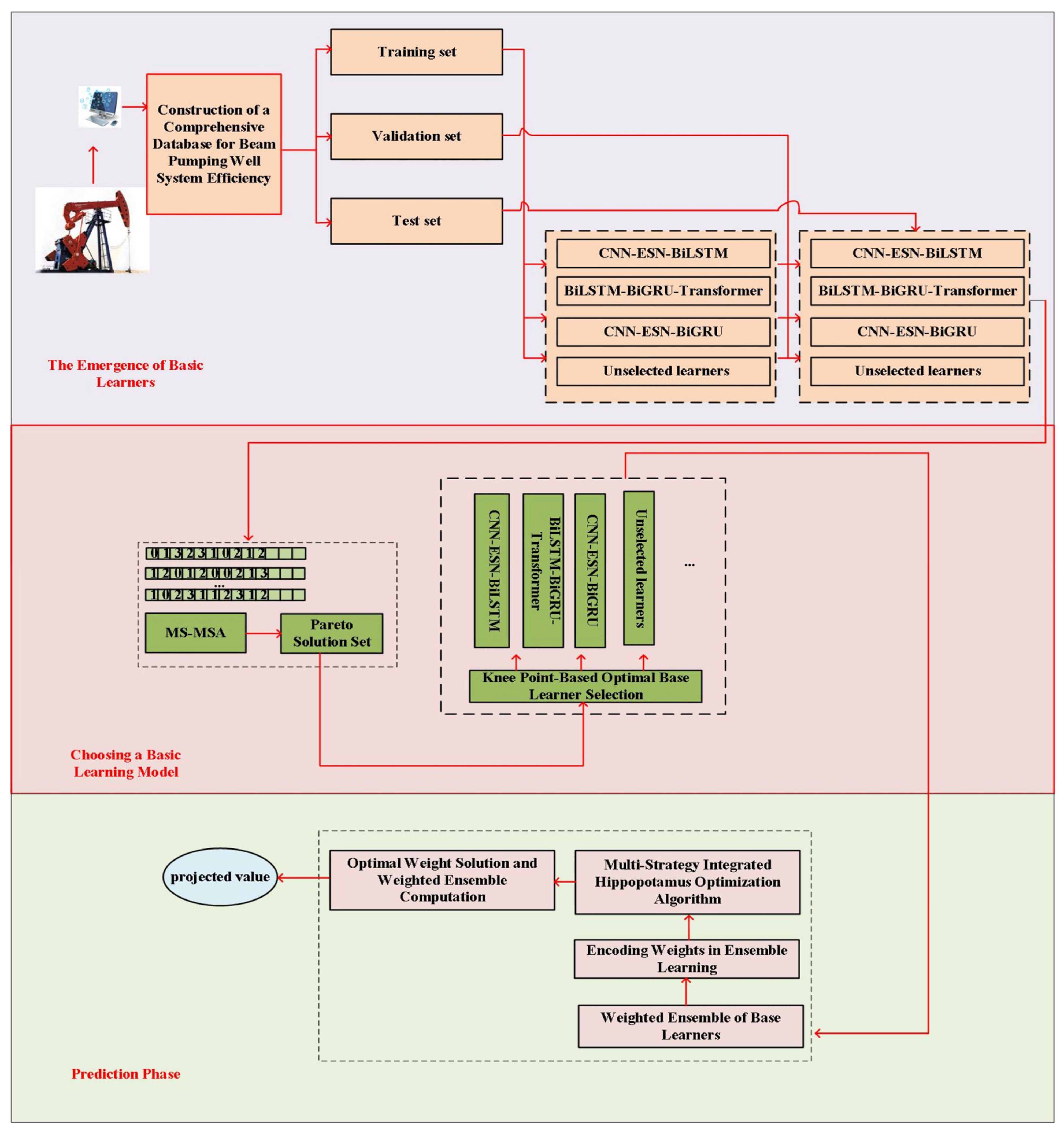
In current ensemble learning methods, base learners are often selected empirically, which restricts model diversity and limits predictive performance. To address these issues, we propose a novel Selective Heterogeneous Ensemble Learning (SHSE) framework. Within this structure, we develop an online surrogate model for estimating rod-pump system efficiency that incorporates three base learners: CNN–ESN–BiLSTM, BiLSTM–BiGRU–Transformer, and CNN–ESN–BiGRU. To balance diversity and accuracy, two multi-strategy meta-heuristic algorithms are employed: a multi-objective Mantis Search Algorithm (MSA) and Hippopotamus Optimization (HO). These algorithms collaboratively optimize the hyperparameters of each base learner, select an optimal subset of models, and determine their ensemble weights. The overall workflow of the SHSE-based surrogate modeling approach is illustrated in Figure 4.

Step 1: Construct the raw dataset from the database and partition it into training, validation, and test sets.

Step 2: Using CNN-ESN-BiLSTM, BiLSTM-BiGRU-Transformer, and CNN-ESN-BiGRU as base learners, randomly select ten base learners and train them on the training set.

Step 3: Let the number of base learners, each learner’s learning rate, network depth, number of neurons per layer, Dropout rate, and weighting coefficients serve as decision variables. Define objective functions that capture both base-learner diversity and predictive accuracy. On the validation set, employ a multi-strategy ensemble–based multi-objective Mantis Search Algorithm to optimize the number of base learners, each learner’s learning rate, network depth, number of neurons per layer, and Dropout rate. Concurrently, use a multi-strategy ensemble–based Hippopotamus Optimization Algorithm to optimize the weighting coefficients. The mathematical formulations for the diversity and accuracy objective functions are given as follows:

$$\left\{\begin{array}{l}MSE={\displaystyle \frac{1}{M}}{\displaystyle \sum _{i=1}^M}{{\displaystyle \left(y_{ac,j}-y_{pr,j}\right)}}^2\\ r={\displaystyle \frac{1}{M-1}}{\displaystyle \sum _{i=1}^M\left(\frac{X_i-\overline{X}}{S_X}\right)}\left({\displaystyle \frac{Y_i-\overline{Y}}{S_Y}}\right)\end{array}\right.$$

(69)

where $M$ represents the total number of samples. $y_{ac,j}$ represents the true values. $y_{pr,j}$ indicates the predicted values. $X_i$ denotes the value $i$ of variable $X$. $Y_i$ refers to the value $i$ of variable $Y$. $\overline{X}$ is the average of variable $X$. $\overline{Y}$ is the average of a variable $Y$. $S_X$ is the standard deviation of $X$. $S_Y$ is the standard deviation of $Y$.

Step 4: Because the multi-strategy ensemble–based multi-objective Mantis Search algorithm produces a Pareto set, a single optimal solution is selected using the knee-point extreme-line method. The mathematical formulation of the knee-point extreme-line method is given as follows:

$$p\times R^2+q\times \rho +b=0$$

(70)

$$d_i={\displaystyle \frac{\left|p\times R^2+q\times \rho +b\right|}{\sqrt{p^2+q^2}}}$$

(71)

$$d_{\max }=\max \left(d_i\right)$$

(72)

where $d_i$ represents the distance from the $i$ optimal solution to the extreme line, and $d_{\max }$ denotes the knee point.

Step 5: Using the optimized hyperparameters obtained previously—including the number of base learners, each learner’s learning rate, network depth, number of neurons per layer, Dropout rate, and weighting coefficients—the model is evaluated on the test set.

4. Experiments

4.1. Data Description

In this study, 3938 operational wells were randomly selected from an custom-built database. The data comprises three types: numerical, string, and sequential. A summary of the sample features is provided in

Table 1. Data characterization.

Characteristics	Example	Characteristics	Example	Characteristics	Example
Pumping unit	YCYJY10-3-48 HB	Pumping speed	4 (min−1)	Downstroke	0.7 mm
Rated power	40 kw	Wellhead pressure	0.8 Mpa	Rod break position	0 m
Saturation pressure	8 MPa	Casinghead pressure	0.6 Mpa	Traveling valve leakage clearance	0 mm
Density	800 kg/m3	Water cut	15%	Standing valve leakage clearance	0 mm
Viscosity	65 (Mpa.s)	Producing fluid level	600 m	Balancing method	Crank balance
GOR	100	Pump clearance	0	Number of centralizers	500
Specific gravity	0.6	Tubing diameter	62 mm	Balance degree	90%
Pump depth	1500 m	Sucker rod grade	3	inclination angle	0.57, 0.57, 0.61, 0.61, 0.49, 0.54, …
Pump diameter	38 mm	Equivalent diameter	23.06 mm	Dogleg severity	0, 6.75990, 5.9005, …
Stroke length	3 m	Upstroke	0	Electric power	2.129928, 2.138211, 2.146494, …
Efficiency	12.67%

. Analysis of Table 1 indicates that the dataset contains 31 features in total, including 30 influencing features and one target feature. The data types are categorized as follows: “Pump Model” and “Balancing Method” are string variables. “Well Inclination,” “Dogleg Severity,” and “Electric Power Profile” are sequential variables. The remaining features are numerical.

4.2. Data Pre-Processing and Evaluation Indicators

To evaluate the prediction accuracy of the proposed approximate models, we partitioned the dataset into 70% training, 15% validation, and 15% test sets. Because each feature represents a specific physical quantity, we applied min-max normalization. The mathematical formulation of min-max normalization is as follows:

$$X={\displaystyle \frac{x-x_{\min }}{x_{\max }-x_{\min }}}$$

(73)

where $x$ is the original data. $x_{\min }$ is the minimum value in the dataset. $x_{\max }$ is the maximum value in the dataset.

We evaluate the multi-strategy-integrated multi-objective Mantis Search Algorithm using three metrics: Generational Distance (GD) quantifies convergence by measuring the average distance from obtained solutions to the true Pareto front; Inverted Generational Distance (IGD) assesses both convergence and diversity by computing the average distance from the true Pareto front to the solution set; and Spacing Metric (SM) evaluates the uniformity of the solution distribution. The mathematical formulations are as follows:

$$GD={\displaystyle \frac{\sqrt{{\displaystyle {\sum }_{i=1}^{N_{obt}}di{s}_i^2}}}{N_{obt}}}$$

(74)

$$MS=\sqrt{{\displaystyle {\sum }_{i=1}^M\max \left(dis\left(a_i,b_i\right)\right)}}$$

(75)

$$GD={\displaystyle \frac{\sqrt{{\displaystyle {\sum }_{i=1}^{N_{\mathrm{true}}}dis{s}_i^2}}}{N_{true}}}$$

(76)

where $N_{obt}$ is Number of obtained PO solutions. $dis$ is Euclidean distance between the I th PO solution obtained and the closest true PO solution in the reference set. $N_{true}$ is Number of true Pareto-optimal solutions. $diss$ is Euclidean distance between the I th true PO solution and the closest PO solution obtained in the reference set. $M$ is Euclidean distance between the I th true PO solution and the closest PO solution obtained in the reference set Number of objectives. $a_i$ and $b_i$ is Maximum and Minimum value of I th objective function.

In this study, the accuracy of the pumpjack well system efficiency prediction model is evaluated using key metrics commonly employed in regression models, including Mean Squared Error (MSE), Root Mean Squared Error (RMSE), Mean Absolute Error (MAE), and the Coefficient of Determination (R²). The mathematical models for these evaluation metrics are as follows:

$$MSE={\displaystyle \frac{1}{M}}{\displaystyle \sum _{i=1}^M}{{\displaystyle \left(y_{ac,j}-y_{pr,j}\right)}}^2$$

(77)

$$RMSE=\sqrt{{\displaystyle \frac{1}{M}}{\displaystyle \sum _{i=1}^M{\left(y_{ac,j}-y_{pr,j}\right)}^2}}$$

(78)

$$MAE={\displaystyle \frac{1}{M}}{\displaystyle \sum _{i=1}^M\left|y_{ac,j}-y_{pr,j}\right|}$$

(79)

$$R^2=1-{\displaystyle \frac{{\displaystyle \sum _{i=1}^M}{{\displaystyle \left(y_{ac,j}-y_{pr,j}\right)}}^2}{{\displaystyle \sum _{i=1}^M}{{\displaystyle \left(\overline{y_{ac,j}}-y_{ac,j}\right)}}^2}}$$

(80)

where $M$ represents the total number of samples. $y_{ac,j}$ the true values. $y_{pr,j}$ the predicted values.

4.3. Experimental Analysis of the Multi-Strategy Integrated Multi-Objective Mantis Search Algorithm

To evaluate the proposed method, we compared it against three baselines—MSSA, MOGOW, and MOMSA—using benchmark functions UF₁–UF₇. Each algorithm was run independently 30 times, and we measured the mean and variance of GD, MS, and IGD. All algorithms used a population size of 100, a maximum of 1000 iterations, and an archive size of 100. The resulting mean and Standard deviation for GD, MS, and IGD are reported in

Table 2. GD statistics for benchmark test.

Function	Index	MSSA	MOGOW	MOMSA	MS-MOMSA
UF1	Ave	0.01410	0.01338	0.01198	0.00520
	Std	0.01290	0.04289	0.00853	0.00120
UF2	Ave	0.00692	0.00378	0.04106	0.00090
	Std	0.00380	0.00337	0.00294	0.00230
UF3	Ave	0.00936	0.05760	0.04153	0.00126
	Std	0.02499	0.03968	0.00931	0.00652
UF4	Ave	0.01700	0.00998	0.01255	0.00786
	Std	0.00439	0.00099	0.00048	0.00035
UF5	Ave	0.03447	0.06425	0.01524	0.01012
	Std	0.03913	0.17316	0.04880	0.00131
UF6	Ave	0.06880	0.06930	0.01680	0.00426
	Std	0.02940	0.01920	0.01670	0.01250
UF7	Ave	0.01325	0.00997	0.00780	0.00610
	Std	0.00677	0.00681	0.00520	0.00396

,

Table 3. IGD Statistics for Test Functions.

Function	Index	MSSA	MOGOW	MOMSA	MS-MOSA
UF1	Ave	0.00490	0.00406	0.00661	0.00309
	Std	0.00030	0.00043	0.00022	0.00011
UF2	Ave	0.00472	0.00334	0.00826	0.00194
	Std	0.00198	0.00052	0.00052	0.00042
UF3	Ave	0.00936	0.05760	0.04153	0.00142
	Std	0.02499	0.03968	0.00931	0.00754
UF4	Ave	0.00749	0.00325	0.00355	0.00256
	Std	0.00163	0.00015	0.00014	0.00012
UF5	Ave	0.04045	0.18600	0.03440	0.02513
	Std	0.04382	0.05046	0.07259	0.00412
UF6	Ave	0.01680	0.01620	0.00584	0.00317
	Std	0.00184	0.00511	0.00136	0.00106
UF7	Ave	0.00610	0.00710	0.00532	0.00361
	Std	0.00023	0.00542	0.00044	0.00010

and

Table 4. MS Statistics for Test Functions.

Function	Index	MSSA	MOGOW	MOMSA	MS-MOSA
UF1	Ave	1.4856	1.1473	0.9936	1.6725
	Std	0.3258	0.6589	0.4279	0.1935
UF2	Ave	1.0100	1.1000	0.8558	1.4580
	Std	0.0527	0.0830	0.0745	0.0213
UF3	Ave	1.4640	1.5700	1.1992	1.7985
	Std	0.7320	0.7429	0.3539	0.2102
UF4	Ave	1.5050	1.0300	1.2044	1.6652
	Std	0.0980	0.0243	0.0232	0.0201
UF5	Ave	1.1173	0.8990	1.2103	1.4780
	Std	0.6825	0.7316	0.7051	0.1540
UF6	Ave	1.4557	0.9560	1.2103	1.6456
	Std	0.3780	0.3290	0.8590	0.2490
UF7	Ave	1.0156	1.0510	1.1121	1.3018
	Std	0.2867	0.3804	0.2920	0.2126

.

We evaluated the proposed Multi-Strategy Multi-Objective Mantis Search Algorithm (MS-MOMSA) on seven benchmark functions (UF₁–UF₇) against three comparative algorithms. As summarized in Table 2, Table 3 and Table 4, MS-MOMSA consistently achieved the lowest mean values in Generational Distance (GD), Inverted Generational Distance (IGD), and Spacing Metric (SM). The superior GD performance demonstrates enhanced convergence capability; the improved IGD reflects a better balance between convergence and diversity; and the leading SM values indicate more uniform distribution and greater coverage of solutions along the Pareto front. These results collectively confirm the effectiveness and robustness of MS-MOMSA in handling complex multi-objective optimization problems.

4.4. Experiments and Analysis of the Multi-Strategy Integrated Hippo Optimization Algorithm (MSHO)

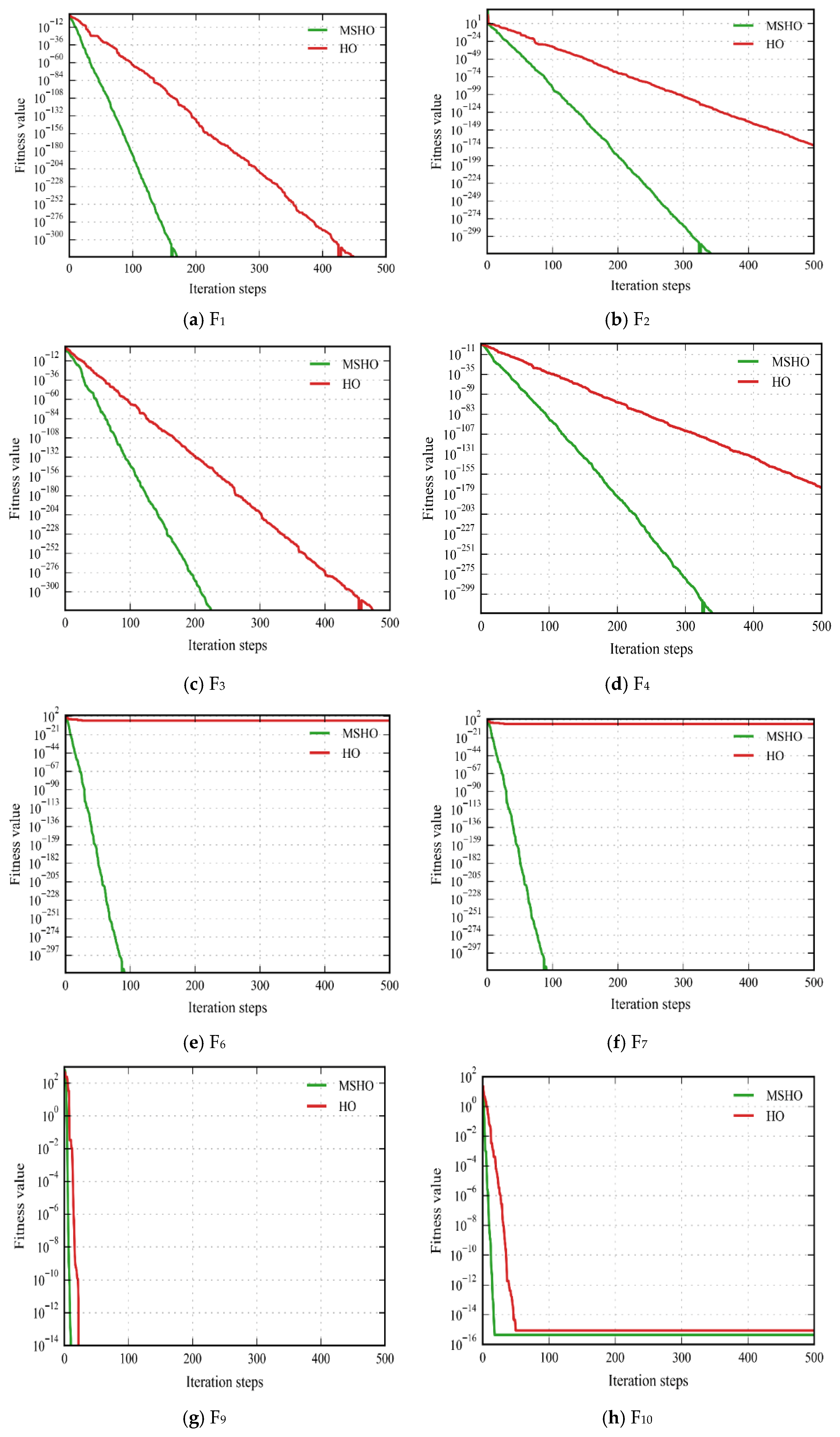
To validate the prediction accuracy of our proposed multi-strategy-enhanced hippopotamus optimization algorithm, we conduct comparative experiments using the conventional hippopotamus optimization algorithm as the baseline model. The evaluation employs eight standard test functions (F₁–F₄, F₆–F₇, F₉–F₁₀) with five performance metrics: mean fitness value, best fitness value, worst fitness value, median fitness value, and fitness variance, all computed over 20 independent runs. The experimental configuration maintains a population size of 24 individuals and 500 maximum iterations for each optimization algorithm. The quantitative results of these performance metrics are systematically presented in

Table 5. Evaluation Metrics for Test Functions.

Function		MSHO	HO	Function		MSHO	HO
F1	Ave	0	0	F2	Ave	0	2.05 × 10−171
	Worst	0	0		Worst	0	3.64 × 10−170
	Median	0	0		Median	0	1.22 × 10−175
	Best	0	0		Best	0	6.71 × 10−185
	Std	0	0		Std	0	0
F3	Ave	0	0	F4	Ave	0	1.3 × 10−172
	Worst	0	0		Worst	0	3.75 × 10−171
	Median	0	0		Median	0	2.98 × 10−177
	Best	0	0		Best	0	2.96 × 10−185
	Std	0	0		Std	0	0
F6	Ave	0	0	F7	Ave	0	0.000392
	Worst	0	0		Worst	0	0.001054
	Median	0	0		Median	0	0.000331
	Best	0	0		Best	0	0.000145
	Std	0	0		Std	0	0.000225
F9	Ave	0	0	F10	Ave	4.441 × 10−16	8.882 × 10−16
	Worst	0	0		Worst	4.441 × 10−16	8.882 × 10−16
	Median	0	0		Median	4.441 × 10−16	8.882 × 10−16
	Best	0	0		Best	4.441 × 10−16	8.882 × 10−16
	Std	0	0		Std	0	0

.

Based on Figure 5 and Table 5, it can be concluded that our proposed multi-strategy integrated Hippo Optimization Algorithm exhibits stronger convergence and higher accuracy compared to the unmodified Hippo Optimization Algorithm.

4.5. Experimental Analysis of Influencing Factors

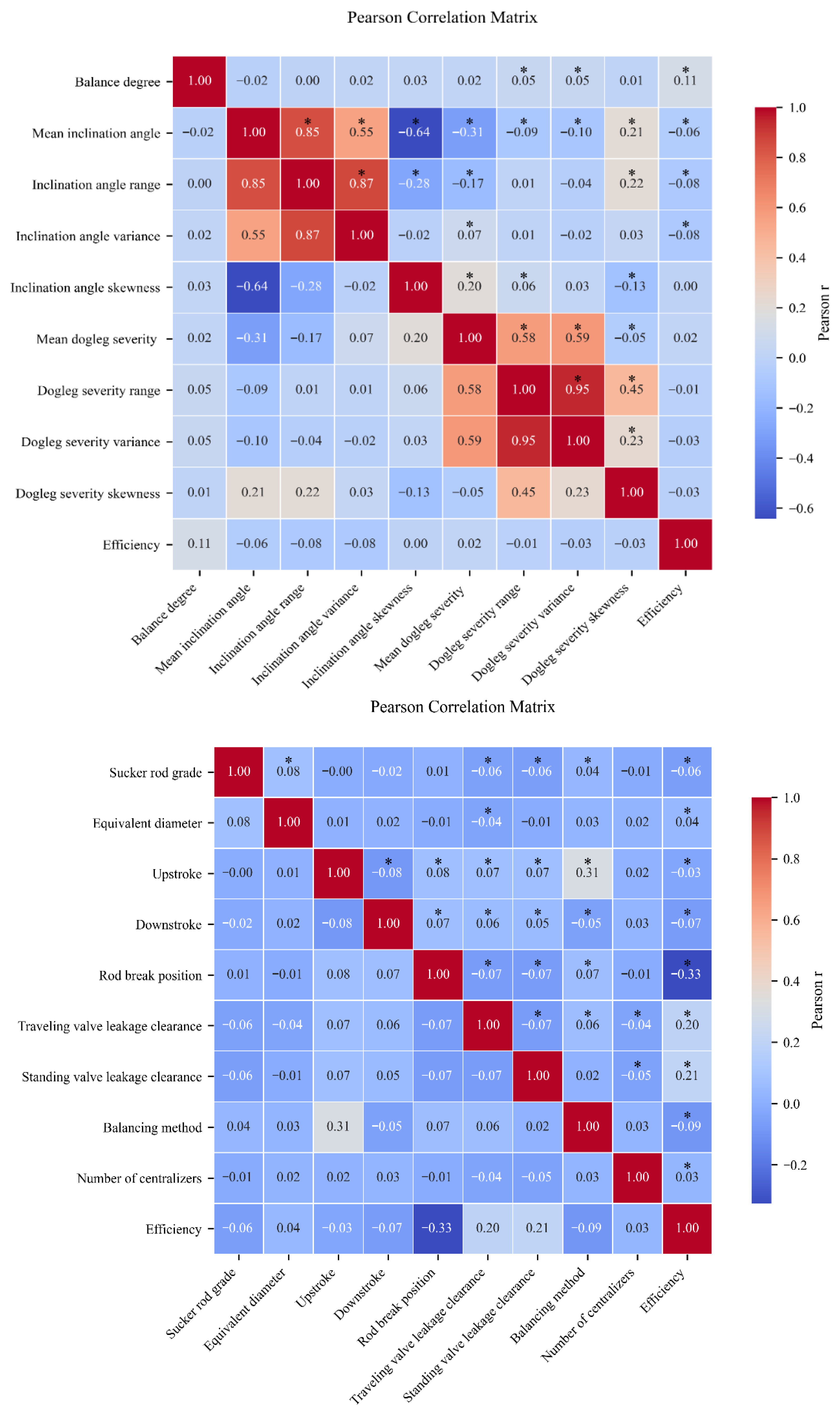
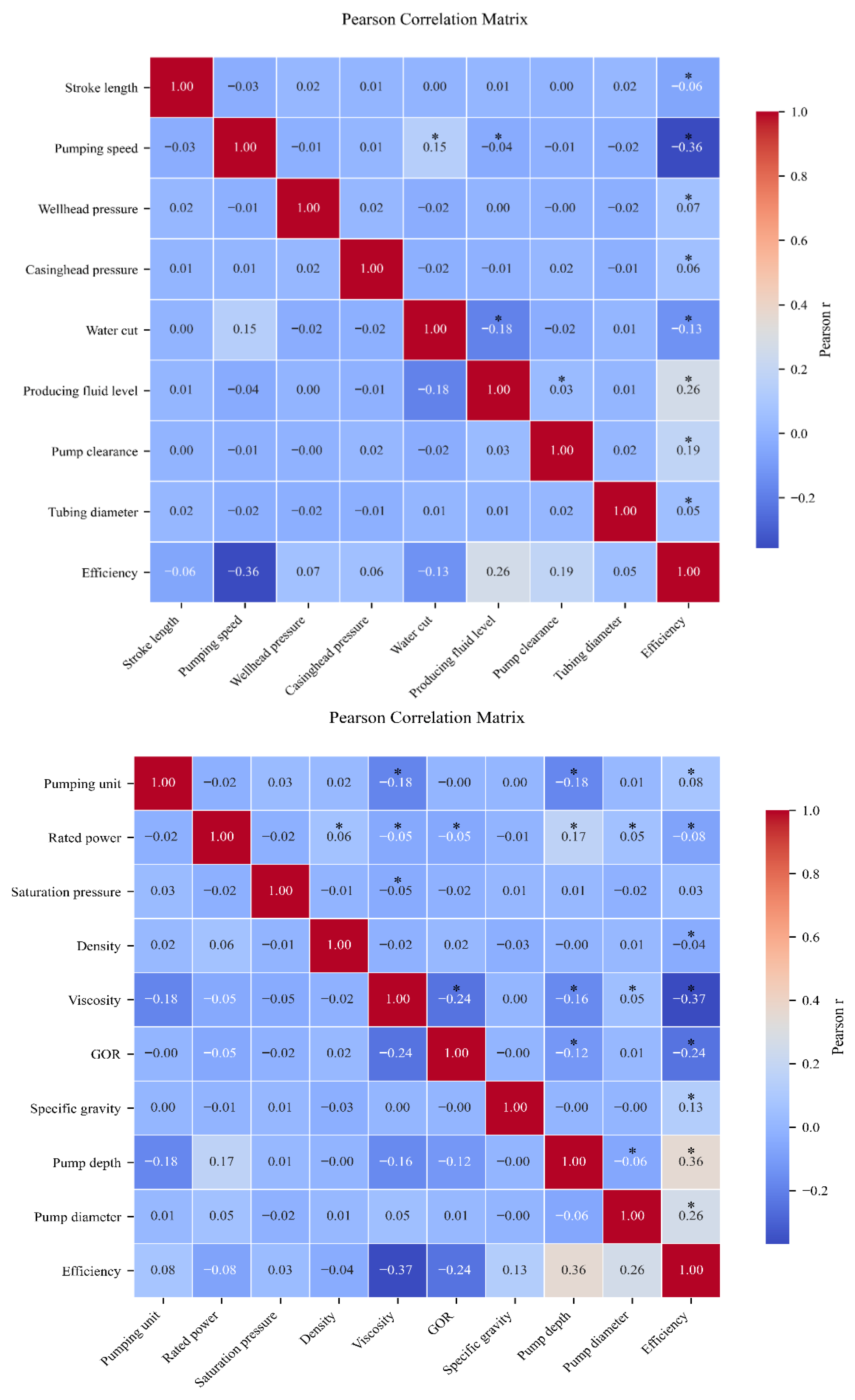
To identify the influential factors, we employ Pearson correlation coefficients and $p$-value significance testing, with the analytical results presented in the following figure.

Because Pearson correlation coefficients quantify the strength of association between each candidate feature and system efficiency, and p-value significance tests determine whether that association is statistically valid, we select only those features for which $\left|r\right|\ne 0$ exceeds the chosen threshold and p < 0.05 as primary predictors. As shown in Figure 6, the selected features include Pumping unit, Rated power, Density, Viscosity, GOR, Specific gravity, Pump depth, Pump diameter, Stroke length, Pumping speed, Wellhead pressure, Casinghead pressure, Water cut, Producing fluid level, Pump clearance, Tubing diameter, Sucker rod grade, Equivalent diameter, Upstroke, Downstroke, Rod break position, Traveling valve leakage clearance, Standing valve leakage clearance, Balancing method, Balance degree, Mean inclination angle, Inclination angle range, Inclination angle variance, Electric power skewness, Electric power kurtosis, and Electric power peak count.

4.6. Experimental Analysis of Approximate Models

To assess the effectiveness of the proposed models, we conducted experiments on the CNN–ESN–BiLSTM, BiLSTM–BiGRU–Transformer, and CNN–ESN–BiGRU architectures, as well as on the selective heterogeneous ensemble–based online soft-measurement method for rod-pump system efficiency.

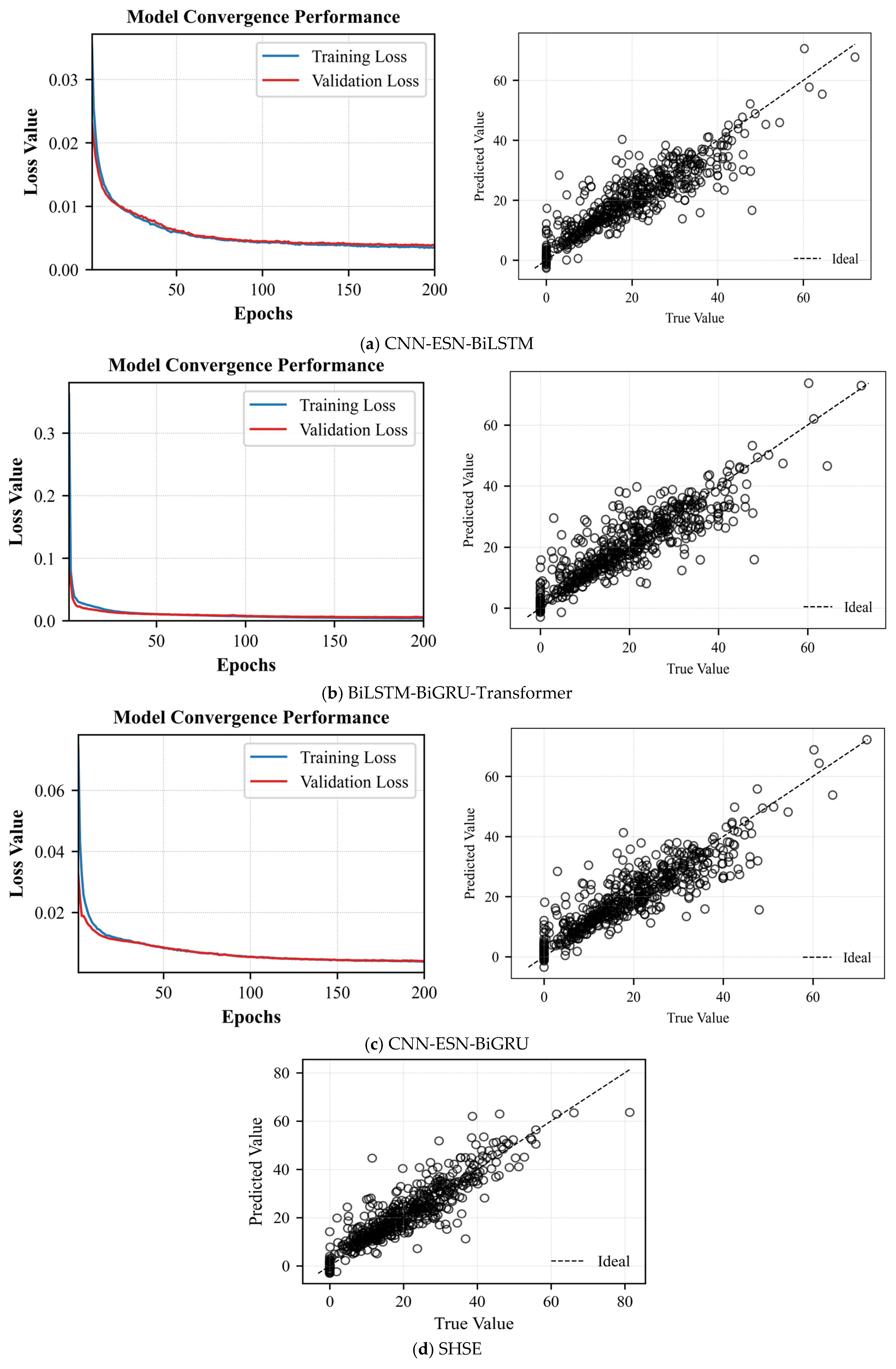
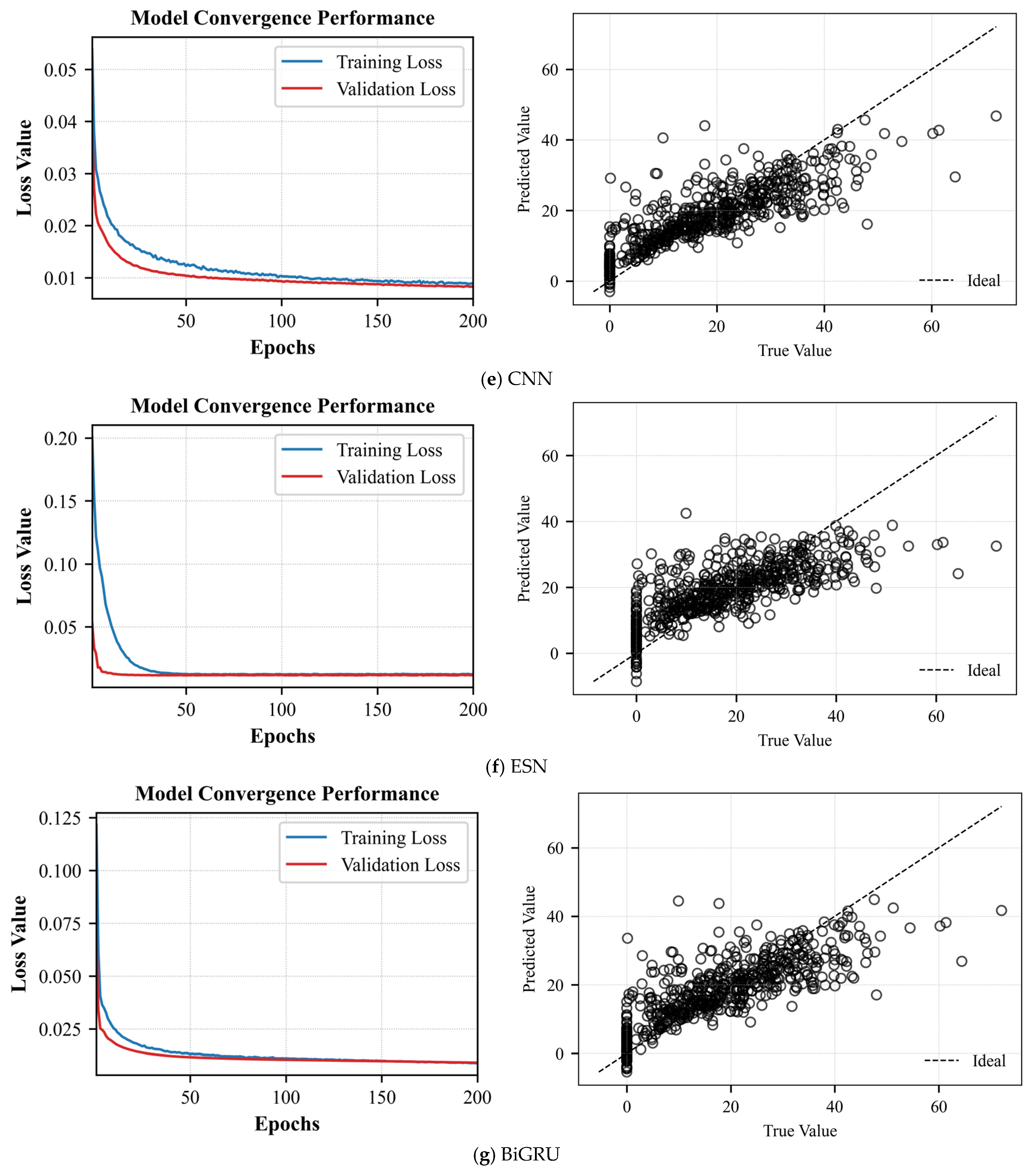
CNN-ESN-BiLSTM: To validate the CNN–ESN–BiLSTM approximate model, we used the following hyperparameters: a learning rate of 0.001, 200 training epochs, a batch size of 500, a single hidden layer with 20 neurons, a dropout rate of 0.5, a reservoir size of 500, a spectral radius of 1.2, an input scaling factor of 1.0, sparsity of 0.2, and a leak rate of 1.0. Figure 7 shows the average loss curves and the mean prediction scatter plots obtained from five experiments.

Table 6. Evaluation Indicators.

Model	MSE	RMSE	R2	MAE
CEBS	0.0038 $\pm$ 0.00019	0.0613 $\pm$ 0.00080	0.8133 $\pm$ 0.00500	0.0425 $\pm$ 0.00054
BBTS	0.0039 $\pm$ 0.00025	0.0624 $\pm$ 0.00199	0.8068 $\pm$ 0.00123	0.0420 $\pm$ 0.00243
CEGS	0.0040 $\pm$ 0.00021	0.0634 $\pm$ 0.00165	0.8006 $\pm$ 0.01036	0.0437 $\pm$ 0.00131
SHSE	0.0031 $\pm$ 0.00011	0.0557 $\pm$ 0.00031	0.8620 $\pm$ 0.00086	0.0358 $\pm$ 0.00019

summarizes the mean evaluation metrics, along with their standard deviations, across the five experiments.

BiLSTM-BiGRU-Transformer: To validate the BiLSTM–BiGRU–Transformer approximate model, the following settings were used: a learning rate of 0.001, 200 training iterations, a batch size of 500, one hidden layer with 10 neurons, and a dropout rate of 0.1. Figure 7 shows the average loss curves and the mean prediction scatter plots obtained from five experiments. Table 6 summarizes the mean evaluation metrics, along with their standard deviations, across the five experiments.

CNN-ESN-BiGRU: To validate the CNN–ESN–BiGRU approximate model, we used a learning rate of 0.001, 200 training iterations, a batch size of 500, one hidden layer with 20 neurons, a dropout rate of 0.5, a reservoir size of 500, a spectral radius of 1.2, an input scaling factor of 1.0, a sparsity of 0.2, and a leak rate of 1.0. Figure 7 shows the average loss curves and the mean prediction scatter plots obtained from five experiments. Table 6 summarizes the mean evaluation metrics, along with their standard deviations, across the five experiments.

SHSE: Since the SHSE approximate model optimizes key hyperparameters—including base learner count, learning rate, hidden neurons per layer, dropout coefficient, hidden layer depth, and weighting coefficients—through MSMOMSA and MSHO algorithms, we configured model parameters as follows: CNN-ESN-BiLSTM: 200 iterations, batch size 500, reservoir size 500, spectral radius 1.2, input scaling 1, sparsity 0.2, leakage rate 1; BiLSTM-BiGRU-Transformer: 200 iterations, batch size 500; CNN-ESN-BiGRU: 200 iterations, batch size 500, reservoir size 500, spectral radius 1.2, input scaling 1, sparsity 0.2, leakage rate 1. For optimization algorithms: MSMOMSA: Population size 10, 100 iterations; MSHOA: Population size 10, 1000 iterations. Figure 7 shows the average loss curves and the mean prediction scatter plots obtained from five experiments. Table 6 summarizes the mean evaluation metrics, along with their standard deviations, across the five experiments.

From Figure 7a and Table 6, it can be observed that both training and validation average losses decrease rapidly within the first 50 epochs, indicating that the model completes the primary parameter tuning during the early stage. Subsequently, the average loss curves continue to decline slowly and eventually stabilize around 0.003–0.005 by the 200th epoch. The training and validation losses maintain a small and stable gap throughout, with no significant divergence or rebound, suggesting that the model does not suffer from severe overfitting or underfitting. The scatter plot points are generally distributed along the diagonal line, covering an efficiency range from 0% to 70%. The model achieves an MSE of 0.0038 ± 0.00019, an RMSE of 0.0613 ± 0.00080, an R² score of 0.8133 ± 0.0050, and a MAE of 0.0425 ± 0.00054. The low MSE, RMSE, and MAE values demonstrate high prediction accuracy, while the R² value exceeding 0.81 confirms that the model explains the majority of the variance in the data. These results collectively indicate that the proposed CEBS model exhibits both robustness and high predictive performance.

From Figure 7b and Table 6, it can be observed that within the first 10 epochs, the average training loss rapidly decreases from its initial value to below 0.01 after only a few iterations and continues to converge quickly toward zero during the subsequent 10–40 epochs. The average validation loss closely follows the average training loss throughout, with the two curves nearly overlapping after 30 epochs and remaining stable at very low values by the end of 200 epochs. Overall, there is no evident divergence or rebound in the average training and average validation losses, indicating that the model does not overfit during training and has sufficient capacity to fit complex functions without signs of underfitting. Most scatter points are concentrated near the diagonal line within the 0–70% efficiency range. The MSE, RMSE, R², and MAE values are 0.0039 $\pm$ 0.00025, 0.0624 $\pm$ 0.00199, 0.8068 $\pm$ 0.00123, and 0.0420 $\pm$ 0.00243, respectively, demonstrating that the proposed soft sensing method achieves low prediction errors with a uniform distribution across the majority of samples.

As shown in Figure 7c and Table 6, the average training loss drops sharply during the first 40 epochs, reaching about 0.01. By epoch 200, the average training and validation losses stabilize around 0.0045 and 0.0050, respectively. The average validation loss closely tracks the average training curve without any notable divergence, indicating strong generalization and absence of overfitting or underfitting. In the scatter plot, predicted versus actual efficiencies cluster tightly around the diagonal across the full range. Quantitatively, the CEGS achieves an MSE of 0.0040 $\pm$ 0.00021, an RMSE of 0.0557 $\pm$ 0.00031, an R² of 0.8620 $\pm$ 0.00086, and an MAE of 0.0358 $\pm$ 0.00019, demonstrating robust linear fitting performance across different efficiency levels.

As shown in Figure 7d and Table 6, most predicted values fall close to the red dashed line over the 0–80% efficiency range. Quantitatively, the model achieves an MSE of 0.0031 $\pm$ 0.00011, an RMSE of 0.0557 $\pm$ 0.00031, an R² of 0.8620 $\pm$ 0.00086, and an MAE of 0.0358 $\pm$ 0.00019, demonstrating a strong linear correlation across all efficiency levels.

4.7. Computational Complexity Analysis

To evaluate the real-time performance of each model, we measured the inference time of the proposed models and the traditional partial differential equation (PDE) solver over five independent runs. The mean and standard deviation were then calculated to ensure statistical reliability. The results are summarized in

Table 7. Inference time.

Model	CEBS	BBTS	CEGS	SHSE	PDE
Parallel Time/ms	1.2539 $\pm$ 0.1678	1.7181 $\pm$ 0.0703	1.4970 $\pm$ 0.1840	1.7359 $\pm$ 0.0649	17,565.5 $\pm$ 1.0124
Serial Time/ms	1.2539 $\pm$ 0.1678	1.7181 $\pm$ 0.0703	1.4970 $\pm$ 0.1840	10.6561 $\pm$ 0.0549	17,565.5 $\pm$ 1.0124

.

As evidenced by the parallel inference times reported in Table 7, the proposed SHSE model substantially reduces computational demands compared to the partial differential equation (PDE)-based approach, demonstrating superior computational efficiency. However, under serial inference settings, SHSE exhibits longer inference times than the three baseline models (CEBS, BBTS, and CEGS), which is attributable to its ensemble architecture that integrates multiple base learners. This design deliberately trades off some computational efficiency for enhanced predictive accuracy. Despite this trade-off, SHSE still maintains considerably higher operational efficiency than traditional PDE-based numerical methods. Furthermore, Table 7 indicates that the serial inference time of SHSE is lower than its parallel execution time, making parallel configuration the preferred option in industrial deployment scenarios to further improve efficiency.

Analysis of model complexity reveals that the parameter counts of the CEBS, BBTS, and CEGS baseline models are 65 K, 91 K, and 86 K, respectively, whereas the SHSE model comprises 523 K parameters. Although SHSE has a significantly larger parameter footprint than each individual baseline model, it achieves corresponding improvements in predictive accuracy, reflecting an effective balance between model capacity and performance.

5. Ablation Study

5.1. Ablation Study of the CNN-ESN-BiLSTM Approximate Model

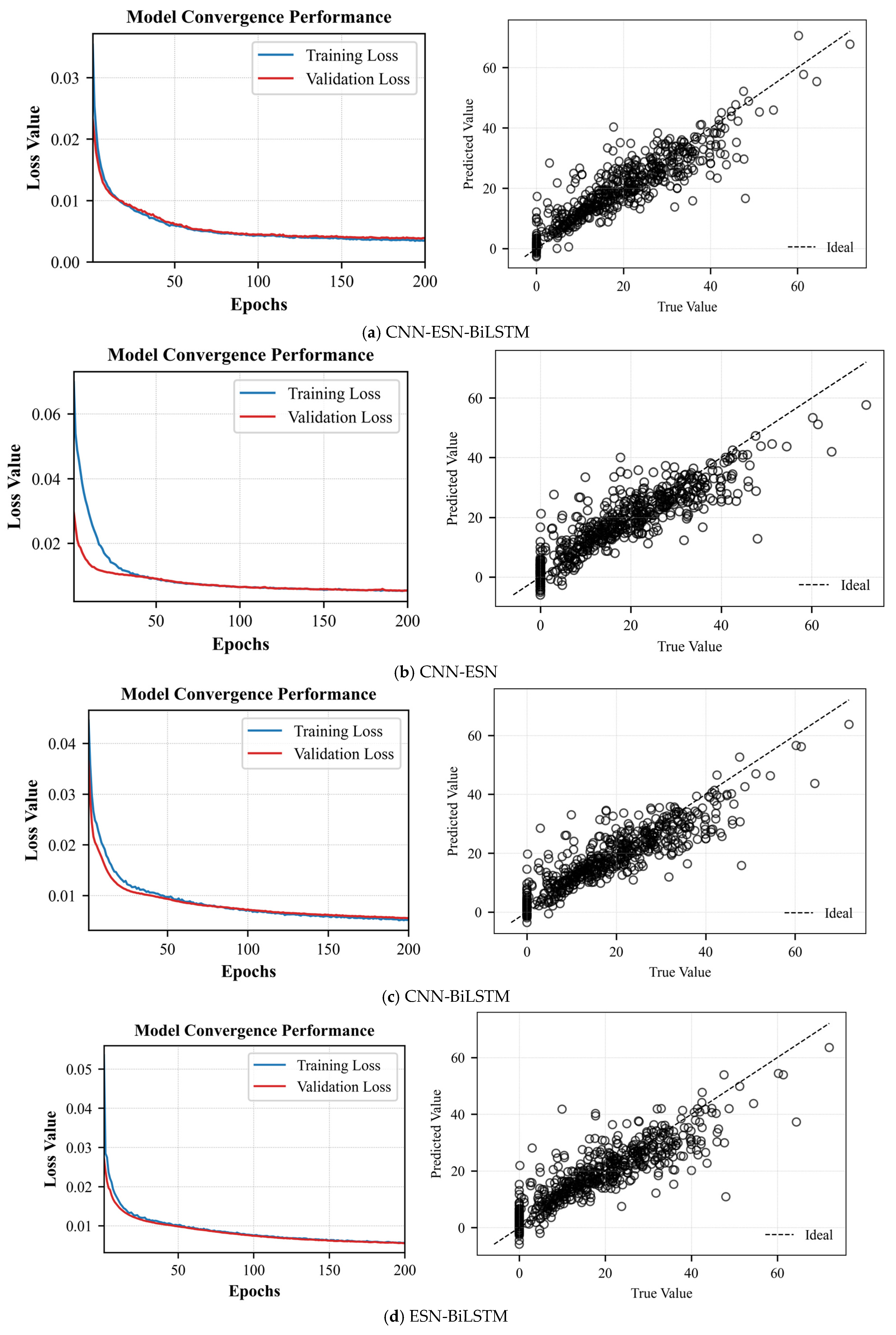
To evaluate the contribution of each component within the CNN-ESN-BiLSTM approximate model to the system efficiency prediction performance, ablation studies were conducted by individually removing the BiLSTM and ESN modules. Each ablated variant was compared against the complete model. We conducted five independent experimental trials.

Table 8. Evaluation Indicators.

Model	MSE	RMSE	R2	MAE
CEBS	0.0038 $\pm$ 0.00019	0.0613 $\pm$ 0.00080	0.8133 $\pm$ 0.00500	0.0425 $\pm$ 0.00054
CNN-ESN	0.0046 $\pm$ 0.00023	0.0679 $\pm$ 0.00170	0.7713 $\pm$ 0.01148	0.0486 $\pm$ 0.00167
CNN-BiLSTM	0.0046 $\pm$ 0.00094	0.0678 $\pm$ 0.00677	0.7698 $\pm$ 0.04655	0.0478 $\pm$ 0.00490
ESN-BiLSTM	0.0049 $\pm$ 0.00015	0.0696 $\pm$ 0.00110	0.7597 $\pm$ 0.00757	0.0489 $\pm$ 0.00080
CNN	0.0068 $\pm$ 0.00080	0.0824 $\pm$ 0.00481	0.6620 $\pm$ 0.03974	0.0604 $\pm$ 0.00439
ESN	0.0095 $\pm$ 0.00035	0.0972 $\pm$ 0.00178	0.5311 $\pm$ 0.01726	0.0735 $\pm$ 0.00164
BiLSTM	0.0063 $\pm$ 0.00063	0.0794 $\pm$ 0.00402	0.6864 $\pm$ 0.03126	0.0553 $\pm$ 0.00273

summarizes the mean and standard deviation of each evaluation metric across all five runs. Figure 8 illustrates the average loss curve over the five trials, along with the corresponding averaged prediction results on the test set.

From Table 8 and Figure 8, it can be observed that the average loss curves for both the training and validation sets of all ablation models show minimal differences, indicating the absence of severe overfitting or underfitting. In the CNN-ESN-BiLSTM prediction model, removing the BiLSTM, ESN, and CNN modules resulted in increases in MSE by 21.05%, 21.05%, and 28.95%, respectively; RMSE increased by 10.77%, 10.60%, and 13.54%, respectively; R² decreased by 5.16%, 5.35%, and 6.59%, respectively; and MAE increased by 14.35%, 12.47%, and 15.06%, respectively. In the CNN-ESN model, further removal of the ESN and CNN modules caused MSE to increase by 47.83% and 106.52%, RMSE by 21.35% and 43.15%, R² to decrease by 14.17% and 31.14%, and MAE to increase by 24.28% and 51.23%, respectively. In the CNN-BiLSTM model, further removal of the BiLSTM and CNN modules led to MSE increases of 47.83% and 36.96%, RMSE increases of 21.53% and 17.11%, R² decreases of 14.00% and 10.83%, and MAE increases of 26.36% and 15.69%, respectively. In the ESN-BiLSTM model, further removal of the BiLSTM and ESN modules resulted in MSE increases of 93.88% and 28.57%, RMSE increases of 39.66% and 14.08%, R² decreases of 30.09% and 9.65%, and MAE increases of 50.31% and 13.09%, respectively. These results indicate that the proposed method effectively integrates the performance of each module.

5.2. BiLSTM-BiGRU-Transformer Approximate Model for Ablation Experiments

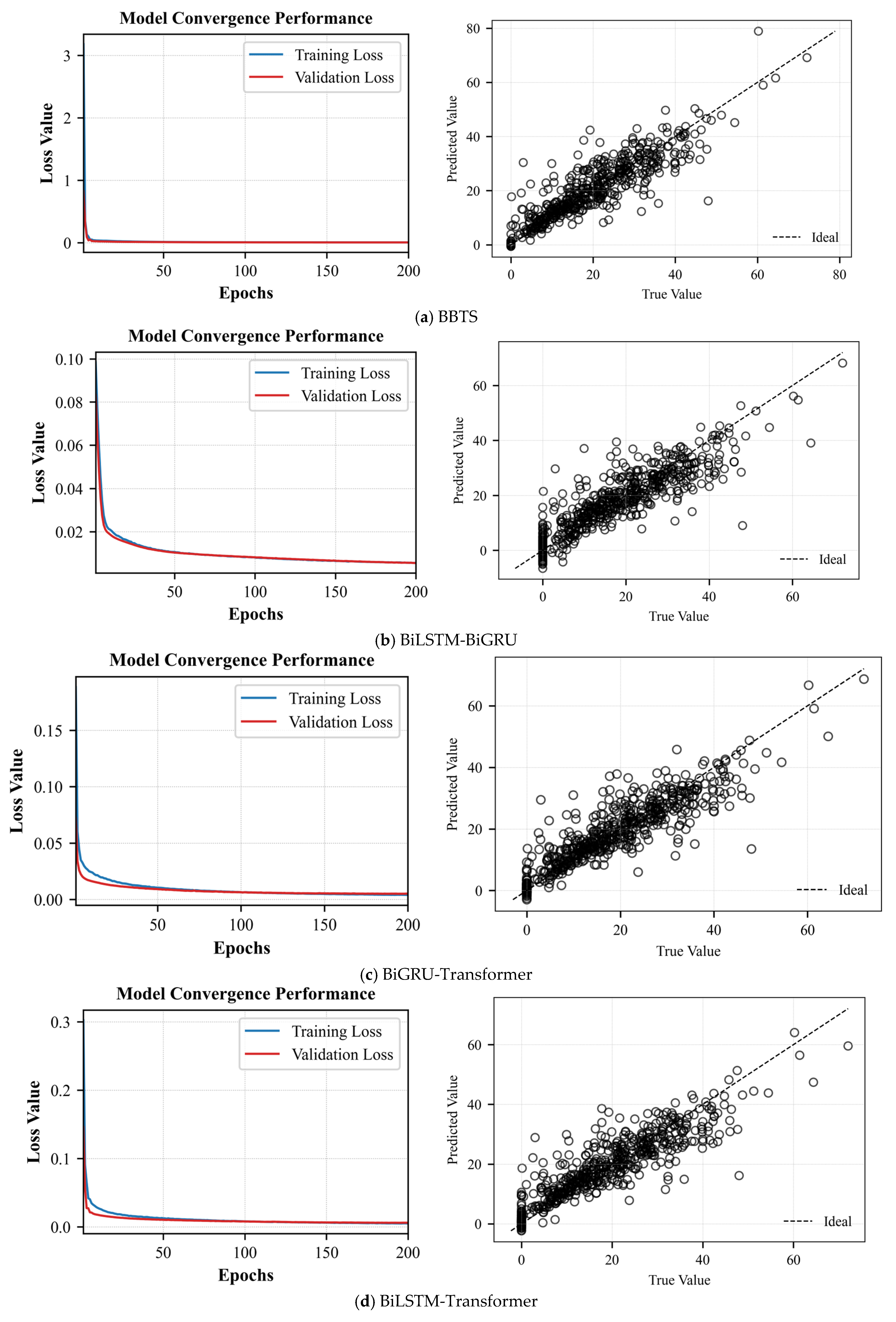
To evaluate the contributions of each component in the BiLSTM-BiGRU-Transformer approximate model to the system efficiency prediction performance, ablation studies were conducted by separately removing the BiGRU and Transformer modules. Each ablated variant was compared with the complete model.

Table 9. Evaluation Indicators.

Model	MSE	RMSE	R2	MAE
BBTS	0.0039 $\pm$ 0.00025	0.0624 $\pm$ 0.00199	0.8068 $\pm$ 0.012398	0.0420 $\pm$ 0.00243
BiLSTM-BiGRU	0.0049 $\pm$ 0.00026	0.0699 $\pm$ 0.00181	0.75728 $\pm$ 0.01265	0.0500 $\pm$ 0.00121
BiGRU-Transformer	0.0047 $\pm$ 0.00028	0.0686 $\pm$ 0.00207	0.76634 $\pm$ 0.01403	0.0470 $\pm$ 0.00175
BiLSTM-Transformer	0.0048 $\pm$ 0.00022	0.0693 $\pm$ 0.00158	0.76142 $\pm$ 0.01091	0.0484 $\pm$ 0.00084
BiLSTM	0.0056 $\pm$ 0.00046	0.0745 $\pm$ 0.00320	0.72392 $\pm$ 0.02301	0.0574 $\pm$ 0.0097
BiGRU	0.0055 $\pm$ 0.00041	0.0741 $\pm$ 0.00271	0.72742 $\pm$ 0.02031	0.0524 $\pm$ 0.00177
Transformer	0.0052 $\pm$ 0.00056	0.0722 $\pm$ 0.00400	0.73562 $\pm$ 0.02780	0.0503 $\pm$ 0.00285

summarizes the mean and standard deviation of each evaluation metric across all five runs. Figure 9 illustrates the average loss curve over the five trials, along with the corresponding averaged prediction results on the test set.

From Table 9 and Figure 9, it can be observed that the loss curves for both the training and validation sets of all ablation models exhibit minimal differences, indicating no significant overfitting or underfitting. In the BiLSTM-BiGRU-Transformer prediction model, the removal of the Transformer, BiLSTM, and BiGRU modules resulted in increases in MSE by 25.64%, 20.51%, and 23.08%, respectively; RMSE increases of 12.02%, 9.94%, and 11.06%; R² decreases of 6.14%, 5.02%, and 5.63%; and MAE increases of 19.05%, 11.90%, and 15.24%, respectively. In the BiLSTM-BiGRU model, further removal of the BiGRU and BiLSTM modules led to MSE increases of 14.29% and 12.24%, RMSE increases of 6.58% and 6.01%, R² decreases of 4.40% and 3.94%, and MAE increases of 14.80% and 4.80%, respectively. In the BiGRU-Transformer model, further removal of the Transformer and BiGRU modules caused MSE increases of 14.55% and 4.08%, RMSE increases of 7.42% and 2.14%, R² decreases of 5.35% and 1.42%, and MAE increases of 10.31% and 2.69%, respectively. In the BiLSTM-Transformer model, further removal of the Transformer and BiLSTM modules resulted in MSE increases of 14.29% and 7.69%, RMSE increases of 6.98% and 4.02%, R² decreases of 5.18% and 3.51%, and MAE increases of 15.68% and 3.78%, respectively. These results indicate that the proposed method effectively integrates the performance of each module.

5.3. CNN-ESN-BiGRU Approximate Model Ablation Experiments

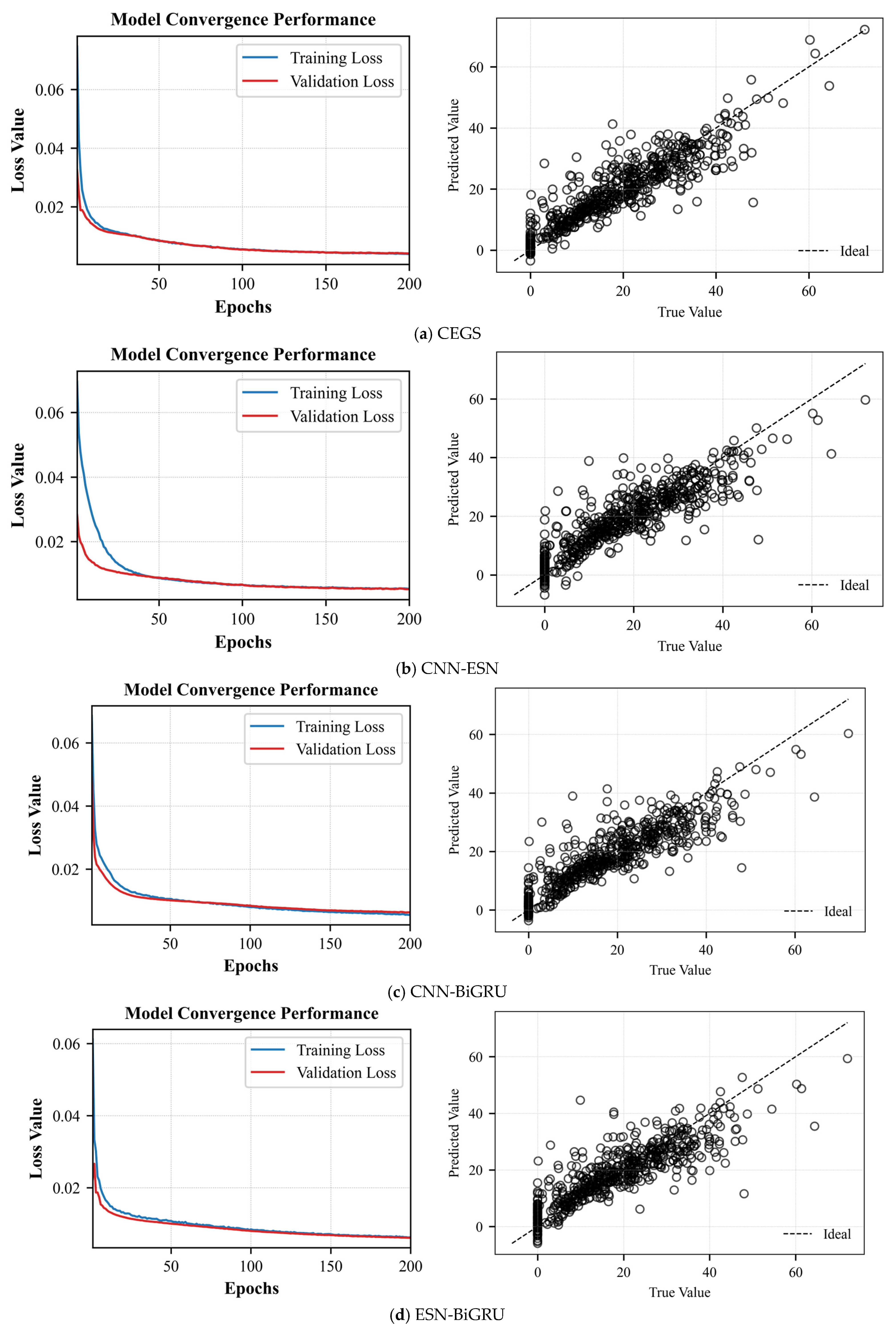
To assess the contribution of each component in the CNN-ESN-BiGRU approximate model to system efficiency prediction performance, ablation experiments were conducted by separately removing the ESN and BiGRU modules for analysis.

Table 10. Evaluation Indicators.

Model	MSE	RMSE	R2	MAE
CEGS	0.0040 $\pm$ 0.00021	0.0634 $\pm$ 0.00165	0.8006 $\pm$ 0.01036	0.0437 $\pm$ 0.00131
CNN-ESN	0.0048 $\pm$ 0.00025	0.0695 $\pm$ 0.00180	0.7603 $\pm$ 0.01214	0.0498 $\pm$ 0.00167
CNN-BiGRU	0.0051 $\pm$ 0.00085	0.0712 $\pm$ 0.00570	0.7466 $\pm$ 0.04206	0.0504 $\pm$ 0.00307
ESN-BiGRU	0.0052 $\pm$ 0.00037	0.0722 $\pm$ 0.00259	0.7413 $\pm$ 0.01830	0.0506 $\pm$ 0.00174
CNN	0.0064 $\pm$ 0.00056	0.0799 $\pm$ 0.00354	0.6827 $\pm$ 0.02796	0.0581 $\pm$ 0.00272
ESN	0.0093 $\pm$ 0.00044	0.0966 $\pm$ 0.00223	0.5365 $\pm$ 0.02164	0.0730 $\pm$ 0.00238
BiGRU	0.0072 $\pm$ 0.00039	0.0849 $\pm$ 0.00229	0.6424 $\pm$ 0.01904	0.0602 $\pm$ 0.00200

summarizes the mean and standard deviation of each evaluation metric across all five runs. Figure 10 illustrates the average loss curve over the five trials, along with the corresponding averaged prediction results on the test set.

Table 10 and Figure 10 show that all ablated variants exhibit nearly identical training and validation loss curves, indicating stable training without overfitting or underfitting. In the full CNN–ESN–BiGRU model, removal of the BiGRU, ESN, and CNN modules increases the MSE by 20.00%, 27.50%, and 30.00%, respectively; the RMSE by 9.62%, 12.30%, and 13.88%; reduces R² by 5.03%, 6.74%, and 7.41%; and raises the MAE by 13.96%, 15.33%, and 15.79%. For the CNN–ESN variant, further ablation of the ESN and CNN modules increases the MSE by 33.33% and 93.75%, the RMSE by 14.96% and 38.99%, reduces R² by 10.21% and 29.44%, and raises the MAE by 16.67% and 46.59%. In the CNN–BiGRU model, removing the BiGRU and CNN modules yields MSE increases of 25.49% and 41.18%, RMSE increases of 12.22% and 19.24%, R² decreases of 8.56% and 13.96%, and MAE increases of 15.28% and 19.44%. Similarly, in the ESN–BiGRU model, ablating the BiGRU and ESN modules results in MSE increases of 78.85% and 38.46%, RMSE increases of 33.80% and 17.59%, R² decreases of 27.63% and 13.34%, and MAE increases of 44.27% and 18.97%. These results confirm that each module—CNN, ESN, and BiGRU—makes a significant, complementary contribution to the overall soft-sensing performance.

5.4. The Impact of Hyperparameters on Model Performance

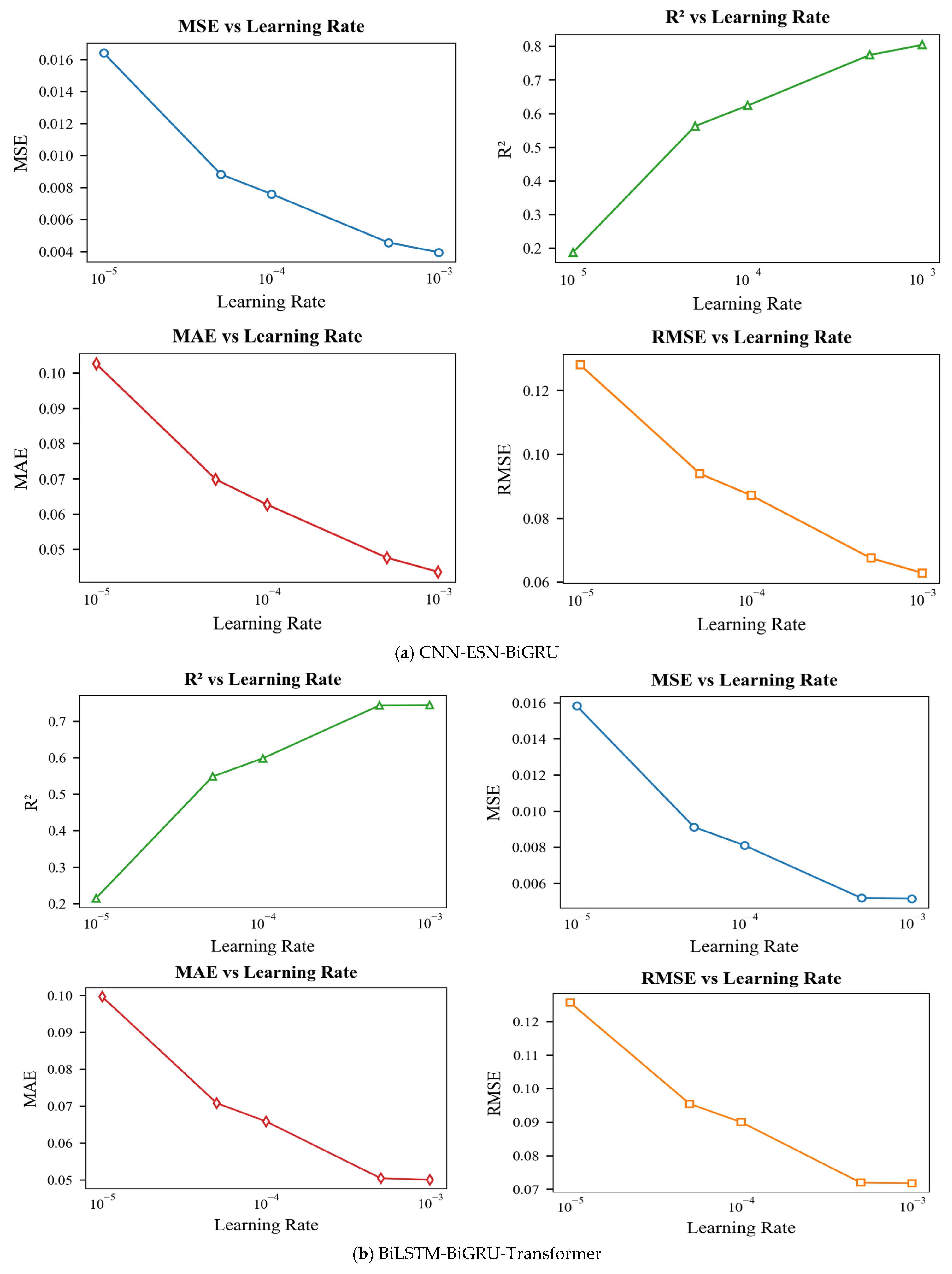
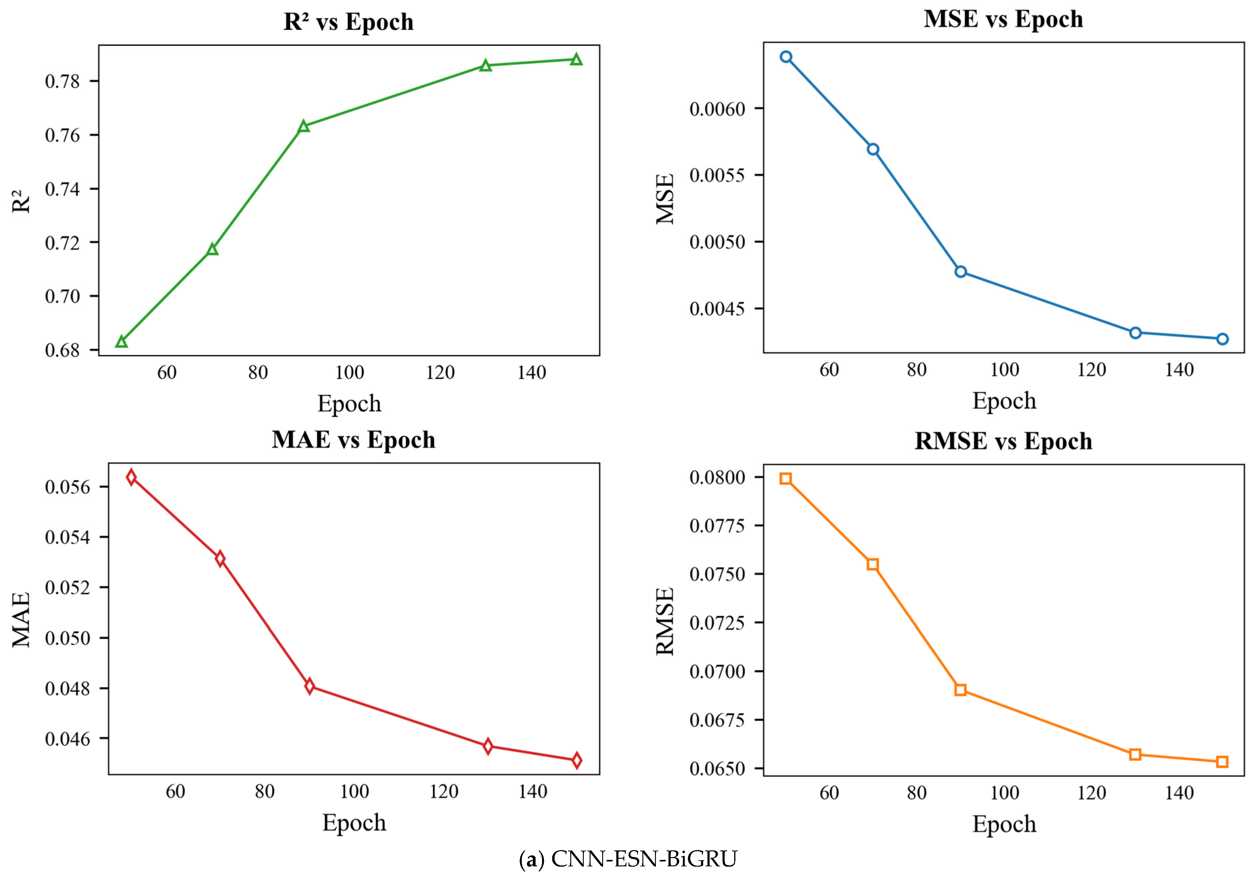
To investigate the influence of key hyperparameters on model performance, we systematically varied the learning rate (0.001, 0.0005, 0.0001, 0.00005, 0.00001) and iteration count (50, 70, 90, 130, 150) based on the baseline configuration in Section 4.6. The resulting performance variations are presented in Figure 11 and Figure 12.

As shown in Figure 11, the MSE, RMSE, and MAE metrics exhibit an initial rapid decline followed by a gradual decrease with increasing learning rates, while the R² metric demonstrates a corresponding pattern of rapid initial improvement transitioning to slower enhancement. This behavior suggests that moderately higher learning rates facilitate more efficient convergence toward the optimal solution. Figure 12 reveals that as the number of iterations increases, the MSE, RMSE, and MAE metrics display consistent monotonic decreases, whereas the R² metric shows a complementary monotonic increase. These observations indicate that extending the training duration effectively enhances the model’s predictive accuracy and fitting capability.

6. Conclusions

The current approximate model for pumping well system efficiency primarily consists of model-based methods and data-driven techniques utilizing historical operational data. While model-based approaches require extensive computational formulations, data-driven methods demand high-quality datasets; both constraints significantly limit real-time efficiency prediction capabilities. To address these challenges, we propose a selective heterogeneous ensemble-based approximate model for system efficiency estimation. The methodology initially performs feature extraction using statistical analysis and one-hot encoding, followed by identification of key influencing factors through Pearson correlation coefficients and significance testing. Subsequently, we develop three hybrid soft sensing architectures: a CNN-ESN-BiLSTM framework, a BiLSTM-BiGRU-Transformer network, and a CNN-ESN-BiGRU model. Furthermore, we develop two enhanced optimization algorithms: a multi-strategy integrated multi-objective mantis search algorithm and a multi-strategy enhanced hippopotamus optimization algorithm. The proposed selective heterogeneous ensemble-based soft sensing method is subsequently constructed by integrating these components. Experimental validation through comprehensive testing and ablation studies demonstrates the method’s superior predictive accuracy for system efficiency estimation, with detailed results confirming its effectiveness.

References

1. Alemi, M.; Jalalifar, H.; Kamali, G.R.; Kalbasi, M.; PEDEC Research and Development. A Mathematical Estimation for Artificial Lift Systems Selection Based on Electre Model. J. Pet. Sci. Eng. 2011, 78, 193–200. [Google Scholar] [CrossRef]
2. Liu, X.F.; Qi, Y.G. A Modern Approach to the Selection of Sucker Rod Pumping System in CBM Wells. J. Pet. Sci. Eng. 2011, 76, 100–108. [Google Scholar] [CrossRef]
3. Mohamed, M.G.; Shedid, A.S.; Mazher, I. Simulation Investigations for Ehanced Performance of Beam Pumping System for Deep. High Volume Wells. In Proceedings of the International Oil Conference and Exhibition in Mexico, Veracruz, Mexico, 27–30 June 2007; Society of Petroleum Engineers: Dallas, TX, USA, 2007. SPE-108284-MS. [Google Scholar]
4. Xu, J.C.; Li, J.H.; Chen, J.; Han, M.; Han, X.; Li, J. Research on Power Saving Positive Torque and Constant Power Pumping Unit and Tracking Tech nique System. In Proceedings of the 2012 International Workshop on Information and Electronics Engineering, Harbin, China, 10–11 March 2012; Elsevier Ltd.: London, UK, 2012; Volume 29, pp. 1034–1041. [Google Scholar]
5. Gibbs, S.G. Predicting the Behavior of Sucker-Rod Pumping Systems. J. Pet. Technol. 1963, 15, 769–778. [Google Scholar] [CrossRef]
6. Langbauer, C.; Antretter, T. Finite Element Based Optimization and Improvement of the Sucker Rod Pumping System. In Proceedings of the Abu Dhabi International Petroleum Exhibition & Conference, Abu Dhabi, United Arab Emirates, 13–16 November 2017. [Google Scholar]
7. Lukasiewicz, S.A. Dynamic Behavior of the Sucker Rod String in the Inclined Well. In Proceedings of the SPE Production Operations Symposium, Oklahoma City, OK, USA, 7–9 April 1991. [Google Scholar]
8. Wang, H.B.; Dong, S.M.; Zhang, Y.; Wang, S.Q.; Sun, X.R. Coupling simulation of the pressure in pump and the longitudinal vibration of sucker rod string based on gas-liquid separation. Shiyou Xuebao/Acta Pet. Sin. 2023, 44, 394–404. [Google Scholar]
9. Xing, M.; Dong, S. An improved longitudinal vibration model and dynamic characteristic of sucker rod string. J. Vibroeng. 2014, 16, 3432–3448. [Google Scholar]
10. Xing, M.M.; Zhou, L.L.; Zhang, C.; Xue, K.; Zhang, Z. Simulation Analysis of Nonlinear Friction of Rod String in Sucker Rod Pumping System. J. Comput. Nonlinear Dyn. 2019, 14, 091008. [Google Scholar] [CrossRef]
11. Li, Q.; Chen, B.; Huang, Z.; Tang, H.; Li, G.; He, L. Study on Equivalent Viscous Damping Coefficient of Sucker Rod Based on the Principle of Equal Friction Loss. Math. Probl. Eng. 2019, 2019, 9272751. [Google Scholar] [CrossRef]
12. Moreno, G.A.; Garriz, A.E. Sucker Rod String Dynamics in Deviated Wells. J. Pet. Sci. Eng. 2020, 184, 106534. [Google Scholar] [CrossRef]
13. Wang, X.B.; Lv, L. Longitudinal vibration analysis of sucker rod based on a simplified thermo-solid model. J. Comput. Nonlinear Dyn. 2021, 196, 107951. [Google Scholar] [CrossRef]
14. Yin, J.-J.; Sun, D.; Yang, Y. Predicting multi-tapered sucker-rod pumping systems with the analytical solution. J. Pet. Sci. Eng. 2021, 197, 108115. [Google Scholar] [CrossRef]
15. Dong, S.; Li, W.; Houtian, B.; Wang, H.; Chen, J.; Liu, M. Optimizing the running parameters of a variable frequency beam pumping system and simulating its dynamic behaviors. Jixie Gongcheng Xuebao/J. Mech. Eng. 2016, 52, 63–70. [Google Scholar] [CrossRef]
16. Wang, H.; Dong, S. Research on the Coupled Axial-Transverse Nonlinear Vibration of Sucker Rod String in Deviated Wells. J. Vib. Eng. Technol. 2021, 9, 115–129. [Google Scholar] [CrossRef]
17. Lekia, S.D.L.; Evans, R.D. A coupled rod and fluid Dynamic model for predicting the behavior of sucker-rod pumping system. SPE Prod. Fac. 1991, 10, 30–45. [Google Scholar]
18. Doty, D.R.; Schmidt, Z. An improved model for sucker rod pumping. SPE J. 1983, 23, 33–41. [Google Scholar] [CrossRef]
19. Ma, B.; Dong, S.M. Coupling Simulation of Longitudinal Vibration of Rod String and Multi-Phase Pipe Flow in Wellbore and Research on Downhole Energy Efficiency. Energies 2023, 16, 4988. [Google Scholar] [CrossRef]
20. Leng, C.Y.; Jia, M.X.; Niu, D.P. Dynamic liquid level prediction for multiple oil wells based on transfer learning and multidimen sional feature fusion network. Meas. Sci. Technol. 2025, 36, 015020. [Google Scholar]
21. Bai, W.P.; Cheng, S.Q.; Wang, Y.; Cai, D.N.; Guo, X.Y.; Guo, Q. A transient production prediction method for tight condensate gas wells with multiphase flow. Pet. Explor. Dev. 2024, 51, 172–179. [Google Scholar] [CrossRef]
22. Wang, Z.-H.; Zhang, X.-K.; Liao, R.-Q.; Ma, Z.-X.; Wang, D.; Yang, W.-X. Measurement of high water-cut heavy oil flow based on differential pressure of swirling flow. Phys. Fluids 2024, 36, 013341. [Google Scholar] [CrossRef]
23. Yang, S.; Li, Y.; Zhang, J.; Yuan, J.; Yang, S.; Ma, X. Interpretable Deep Learning Approach for Production Forecasting of Fractured Horizontal Wells. Chem. Technol. Fuels Oils 2024, 60, 391–399. [Google Scholar] [CrossRef]
24. Qu, F.; Liao, H.; Lu, M.; Niu, W.; Shi, F. Recognition of drill string vibration state based on WGAN-div and CNN-IWPSO-SVM. Geoenergy Sci. Eng. 2024, 243, 213342. [Google Scholar] [CrossRef]
25. Zhang, X.; Lu, Y.-H.; Jin, Y.; Chen, M.; Zhou, B. An adaptive physics-informed deep learning method for pore pressure prediction using seismic data. Pet. Sci. 2024, 21, 885–902. [Google Scholar] [CrossRef]
26. Sørensen, R.B.; Nielsen, J.J.; Popovski, P. Machine Learning Methods for Monitoring of Quasiperiodic Traffic in Massive IoT Networks. IEEE Internet Things J. 2020, 7, 7368–7376. [Google Scholar] [CrossRef]
27. Yan, W.; Tang, D.; Lin, Y. A Data-Driven Soft Sensor Modeling Method Based on Deep Learning and its Application. IEEE Trans. Ind. Electron. 2017, 64, 4237–4245. [Google Scholar] [CrossRef]
28. Ren, L.; Wang, T.; Laili, Y.; Zhang, L. A Data-Driven Self-Supervised LSTM-DeepFM Model for Industrial Soft Sensor. IEEE Trans. Ind. Informatics. 2022, 18, 5859–5869. [Google Scholar] [CrossRef]
29. Lui, C.F.; Liu, Y.; Xie, M. A Supervised Bidirectional Long Short-Term Memory Network for Data-Driven Dynamic Soft Sensor Modeling. IEEE Trans. Instrum. Meas. 2022, 71, 2504713. [Google Scholar] [CrossRef]
30. Guo, R.; Liu, H. A Hybrid Mechanism- and Data-Driven Soft Sensor Based on the Generative Adversarial Network and Gated Recurrent Unit. IEEE Sens. J. 2021, 21, 25901–25911. [Google Scholar] [CrossRef]
31. Lu, Q.Y.; Wang, S.L.; Jang, M.Z. Main control factors affecting mechanical oil recovery efficiency in complex blocks identified using the improved K-means algorithm. PLoS ONE 2021, 16, e0248840. [Google Scholar] [CrossRef] [PubMed]
32. Tan, C.D.; Deng, H.W.; Feng, Z.M. Data-driven system efficiency prediction production parameter optimization for, PW-LHM. J. Pet. Sci. Eng. 2022, 209, 109810. [Google Scholar] [CrossRef]
33. Ma, B.; Dong, S. Anovel hybrid efficiency prediction model for pumping well system based on MDS–SSA–GNN. Energy Sci. Eng. 2024, 12, 3272–3288. [Google Scholar] [CrossRef]
34. Ma, B.; Dong, S. A Hybrid Prediction Model for Pumping Well System Efficiency Based on Stacking Integration Strategy. Int. J. Energy Res. 2024, 2024, 8868949. [Google Scholar] [CrossRef]
35. Tan, M.; Yuan, S.; Li, S.; Su, Y.; Li, H.; He, F. Ultra-Short-Term Industrial Power Demand Forecasting Using LSTM Based Hybrid Ensemble Learning. IEEE Trans. Power Syst. 2020, 35, 2937–2948. [Google Scholar] [CrossRef]
36. Huang, D.; Wang, C.D.; Peng, H.; Lai, J.; Kwoh, C.K. Enhanced Ensemble Clustering via Fast Propagation of Cluster-Wise Similarities. IEEE Trans. Syst. Man Cybern. Syst. 2021, 51, 508–520. [Google Scholar] [CrossRef]
37. Gao, R.; Hu, M.; Li, R.; Luo, X.; Suganthan, P.N.; Tanveer, M. Stacked Ensemble Deep Random Vector Functional Link Network with Residual Learning for Medium-Scale Time-Series Forecasting. IEEE Trans. Neural Netw. Learn. Systems 2025, 36, 10833–10843. [Google Scholar] [CrossRef]
38. Naresh, V.S.; Gayathri, P.; Tejaswi, P.; Induja, P.; Reddy, C.R.; Sudheer, Y. Optimizing electric vehicle battery health monitoring: A resilient ensemble learning approach for state-of-health prediction. Sustain. Energy Grids Netw. 2025, 42, 101655. [Google Scholar] [CrossRef]
39. Dahal, A.; Moulik, S.; Mukherjee, R. Stack-HAR: Complex Human Activity Recognition with Stacking-Based Ensemble Learning Framework. IEEE Sens. J. 2025, 25, 16373–16380. [Google Scholar] [CrossRef]
40. Wang, W.-C.; Gu, M.; Li, Z.; Hong, Y.-H.; Zang, H.-F.; Xu, D.-M. A stacking ensemble machine learning model for improving monthly runoff prediction. Earth Sci. Inform. 2025, 18, 120. [Google Scholar] [CrossRef]
41. Yun, F.; Yu, Z.; Yang, K.; Chen, C.P. AdaBoost-Stacking Based on Incremental Broad Learning System. IEEE Trans. Knowl. Data Eng. 2024, 36, 7585–7599. [Google Scholar] [CrossRef]
42. Guo, Y.; Wang, X.; Xiao, P.; Xu, X. An ensemble learning framework for convolutional neural network based on multiple classifiers. Soft Comput. 2020, 24, 3727–3735. [Google Scholar] [CrossRef]
43. Nai, K.; Chen, S. Learning a Novel Ensemble Tracker for Robust Visual Tracking. IEEE Trans. Multimed. 2024, 26, 3194–3206. [Google Scholar] [CrossRef]
44. Li, L.; Zheng, H. Multidomain Transfer Ensemble Learning for Wireless Fingerprinting Localization. IEEE Internet Things J. 2024, 11, 11693–11706. [Google Scholar] [CrossRef]
45. Peng, W.; Lei, J.; Ding, C.; Yue, C.; Ma, G.; Sun, J.; Zhang, D. A novel deep ensemble reinforcement learning based control method for strip flatness in cold rolling steel industry. Eng. Appl. Artif. Intell. 2024, 134, 108695. [Google Scholar] [CrossRef]
46. Yu, X.; Peng, Q.; Xu, L.; Jiang, F.; Du, J.; Gong, D. A selective ensemble learning based two-sided cross-domain collaborative filtering algorithm. Inf. Process. Manag. 2021, 58, 102691. [Google Scholar] [CrossRef]
47. Zhang, S.X.; Liu, Y.H.; Zheng, L.M.; Zheng, S.Y. Differential evolution with collective ensemble learning. Swarm Evol. Comput. 2024, 87, 101521. [Google Scholar] [CrossRef]
48. Dai, Q.; Zhou, X.; Yang, J.-P.; Du, T.; Chen, L.-F. A mutually supervised heterogeneous selective ensemble learning framework based on matrix decomposition for class imbalance problem. Expert Syst. Appl. 2025, 271, 126728. [Google Scholar] [CrossRef]
49. Jameel, M.; Abouhawwash, M. Multi-objective Mantis Search Algorithm (MOMSA): A novel approach for engineering design problems and validation. Comput. Methods Appl. Mech. Eng. 2024, 422, 116840. [Google Scholar] [CrossRef]
50. Amiri, M.H.; Hashjin, N.M.; Montazeri, M.; Mirjalili, S.; Khodadadi, N. Hippopotamus optimization algorithm: A novel nature-inspired optimization algorithm. Sci. Rep. 2024, 14, 5032. [Google Scholar] [CrossRef]
Figure 1. CNN-ESN-BiLSTM–based online soft measurement method for rod-pump system efficiency.
Fractalfract 09 00660 g001
Figure 2. BiLSTM–BiGRU–Transformer–based online soft measurement method for rod-pump system efficiency.
Fractalfract 09 00660 g002
Figure 3. Online Soft-Sensing Method for Sucker-Rod Pumping System Efficiency Based on CNN-ESN-BiGRU.
Fractalfract 09 00660 g003
Figure 4. Online Soft-Sensing Method for Sucker-Rod Pumping System Efficiency Based on Selective Heterogeneous Ensemble.
Fractalfract 09 00660 g004
Figure 5. Iteration comparison for each test function.
Fractalfract 09 00660 g005
Figure 6. Pearson’s correlation coefficient and significance test. * indicates p < 0.05.
Fractalfract 09 00660 g006aFractalfract 09 00660 g006bFractalfract 09 00660 g006c
Figure 7. Average Loss Function and Average Prediction Map.
Fractalfract 09 00660 g007
Figure 8. Average Loss Function and Prediction Scatter Plot.
Fractalfract 09 00660 g008aFractalfract 09 00660 g008b
Figure 9. Average Loss Function and Prediction Scatter Plot.
Fractalfract 09 00660 g009aFractalfract 09 00660 g009b
Figure 10. Average Loss Function and Prediction Scatter Plot.
Fractalfract 09 00660 g010aFractalfract 09 00660 g010b
Figure 11. Evaluation Metrics as a Function of Learning Rate.
Fractalfract 09 00660 g011aFractalfract 09 00660 g011b
Figure 12. Evaluation Metric Variation with Epoch.
Fractalfract 09 00660 g012aFractalfract 09 00660 g012b