Article

Hybrid Fuzzy Fractional for Multi-Phasic Epidemics: The Omicron–Malaria Case Study

1
Department of Mathematics, College of Science, University of Ha’il, Ha’il 55473, Saudi Arabia
2
Biology Department, College of Science, Imam Mohammad Ibn Saud Islamic University (IMSIU), Riyadh 11432, Saudi Arabia
3
Department of Mathemtaics, College of Computer and Information Technology, Alrazi University, Sana’a 72738, Yemen
4
Department of Mathematics, Faculty of Science, Islamic University of Madinah, Madinah 42351, Saudi Arabia
5
Department of Mathematics, University College of Umluj, University of Tabuk, Tabuk 48322, Saudi Arabia
6
Department of Mathematics, College of Science, Qassim University, Buraydah 51452, Saudi Arabia
7
Department of Mathematics and Statistics, Imam Mohammad Ibn Saud Islamic University (IMSIU), Riyadh 11432, Saudi Arabia
*
Authors to whom correspondence should be addressed.
Fractal Fract. 2025, 9(10), 643; https://doi.org/10.3390/fractalfract9100643
Submission received: 27 August 2025 / Revised: 13 September 2025 / Accepted: 23 September 2025 / Published: 1 October 2025

Abstract

This study introduces a novel Fuzzy Piecewise Fractional Derivative (FPFD) framework to enhance epidemiological modeling, specifically for the multi-phasic co-infection dynamics of Omicron and malaria. We address the limitations of traditional models by incorporating two key realities. First, we use fuzzy set theory to manage the inherent uncertainty in biological parameters. Second, we employ piecewise fractional operators to capture the dynamic, phase-dependent nature of epidemics. The framework utilizes a fuzzy classical derivative for initial memoryless spread and transitions to a fuzzy Atangana–Baleanu–Caputo (ABC) fractional derivative to capture post-intervention memory effects. We establish the mathematical rigor of the FPFD model through proofs of positivity, boundedness, and stability of equilibrium points, including the basic reproductive number (R0). A hybrid numerical scheme, combining Fuzzy Runge–Kutta and Fuzzy Fractional Adams–Bashforth–Moulton algorithms, is developed for solving the system. Simulations show that the framework successfully models dynamic shifts while propagating uncertainty. This provides forecasts that are more robust and practical, directly informing public health interventions.

1. Introduction

Mathematical modeling has become an indispensable tool in epidemiology, providing critical insights into the transmission dynamics of infectious diseases and helping to evaluate the potential impact of public health interventions [1,2,3,4]. The pursuit of mathematical epidemiology has entered a new era of complexity, moving beyond the classical objective of fitting models to data. The central challenge now lies in creating frameworks that can faithfully represent the two fundamental realities of modern epidemics: their dynamic non-stationarity and their inherent uncertainty. Real-world outbreaks are not monolithic events governed by a single, unchanging law. They are multi-phasic, marked by distinct structural breaks driven by public health interventions, the evolution of pathogen virulence, or shifts in population behavior [5,6,7]. A model that cannot adapt its dynamics across these phases risks generating forecasts that are not just inaccurate but dangerously misleading. Conventional mathematical models, whether integer-order or standard fractional-order, are built on the implicit assumption of a stationary dynamic process [8,9,10]. They apply a single mathematical operator across the entire timeline of an epidemic. This approach is ill-equipped to capture the profound system-wide shifts that occur, for example, when a widespread vaccination campaign is launched or when a new, more transmissible variant displaces its predecessor.
To address this limitation, a more sophisticated approach is required, one that allows the model itself to transition between different dynamic regimes. The concept of piecewise differential operators, recently introduced to model crossover behaviors [11,12,13,14], offers a powerful solution. It enables a system to switch its governing principles, for instance, from a memoryless state before an intervention to a memory-dependent state afterward, thereby reflecting the long-term impact of the change [15,16,17,18].
Parallel to this challenge of temporal dynamics is the equally critical issue of epistemic uncertainty. The parameters that define an epidemic model are never known with perfect precision, often being derived from noisy or incomplete data. Deterministic models that rely on single-point values ignore this inherent vagueness. Fuzzy set theory, pioneered by Zadeh [19], provides a rigorous mathematical language to formally incorporate and manage this type of uncertainty. By representing parameters and state variables as fuzzy numbers, we can develop models whose solutions are not single curves but “solution bands,” encapsulating a spectrum of possible outcomes [20,21]. This approach provides a far more honest and practical forecast, equipping policymakers with a quantitative understanding of best-case, worst-case, and most-likely scenarios [22]. This approach has proven particularly potent in medical contexts, from enhancing the analysis of diagnostic data [23] to structuring complex medicine selection problems and group decision-making processes [24,25]. Furthermore, advanced operators like the Atangana–Baleanu fractional derivative have been successfully integrated with fuzzy concepts [26]. This success motivates our development of the more comprehensive framework proposed in this work.
Neither the piecewise nor the fuzzy approach alone, however, can fully resolve the dual challenges of modern epidemiological modeling. A framework is needed that can simultaneously manage both structural breaks in time and persistent uncertainty in data. This paper introduces such a framework: the Fuzzy Piecewise Fractional Derivative (FPFD). This novel mathematical structure synthesizes two powerful tools: the adaptability of piecewise operators [27,28] and the ability of fuzzy calculus to quantify uncertainty [29,30,31]. This FPFD framework is uniquely suited to model the complex, multi-stage, and data-scarce environments that characterize emerging infectious disease threats. To demonstrate the power and practical utility of this new framework, we apply it to the complex clinical challenge of Omicron and malaria co-infection [32]. This scenario provides a demanding test case, involving the interplay of a highly transmissible respiratory virus (a variant of SARS-CoV-2) and a vector-borne parasitic disease with distinct pathologies and transmission routes. The potential for synergistic effects, where one disease exacerbates the other, makes this a critical area of study, particularly in regions where both diseases are endemic.
While previous studies have explored fractional-order models for co-infection (e.g., [32]) and fuzzy models for single diseases (e.g., [33]), no existing work has integrated piecewise dynamics with a fuzzy fractional framework to tackle a multi-phasic co-infection problem. This gap highlights the need for novel mathematical structures capable of addressing modern challenges, a trend seen in other areas of health technology, such as the use of fractal-based methods for analyzing the complexity of COVID-19 medical imagery [34]. Our work aims to fill this specific void by introducing a tailored, robust framework. The primary contributions of this paper are therefore threefold:
  • Methodological Innovation: We introduce and formally define the Fuzzy Piecewise Fractional Derivative (FPFD) framework. This involves establishing the theoretical underpinnings for a model that can switch its governing mathematical operator in a fuzzy environment, providing a new, powerful tool for applied mathematicians and modelers.
  • Rigorous Analytical and Numerical Development: We provide a comprehensive analysis of the proposed FPFD co-infection model, including proofs of the existence, uniqueness, positivity, and boundedness of the solutions. We also design and implement a novel hybrid numerical scheme (combining Fuzzy Runge–Kutta and Fuzzy Adams-Bashforth methods) that can accurately solve such piecewise systems.
  • Practical Application and Policy Translation: We demonstrate the framework’s utility by applying it to the Omicron–malaria co-infection scenario. Crucially, we move beyond a purely mathematical discussion by providing a direct interpretation of the model’s fuzzy, interval-valued outputs for public health policy, showcasing how this approach can support more robust and risk-aware strategic planning in the face of complex epidemiological threats.
This work aims to bridge the gap between advanced mathematical theory and practical epidemiological application, laying the groundwork for a new class of models better suited to the uncertain and dynamic nature of the real world.

2. Preliminaries

In this section, we outline the key mathematical concepts that directly underpin our novel Fuzzy Piecewise Fractional Derivative (FPFD) operator [35,36,37,38]. For the convenience of the reader, more foundational definitions regarding fuzzy numbers, the generalized Hukuhara difference, and the standard fuzzy classical and ABC fractional derivatives have been moved to Appendix A. Here, we present only the most essential theorem that governs the existence of solutions for fuzzy differential equations.
The theoretical properties of fuzzy-valued functions provide the rigorous foundation for the fuzzy calculus we develop. The behavior of such functions has been a subject of extensive study, with recent work exploring generalized fuzzy-valued convexity and its application in establishing powerful inequalities over inclusion relations [39]. Furthermore, the fundamental structure of fuzzy spaces, including the properties of convergent sequences within fuzzy normed spaces [40], ensures that the analytical and numerical methods applied in this paper are well-posed and mathematically sound.
We will rely on the fuzzy extension of the Picard–Lindelöf theorem to establish the existence and uniqueness of solutions in the classical part of our piecewise model.
Theorem 1
(Fuzzy Picard–Lindelöf). Let F : [ 0 , t 1 ) × D R F n be a mapping where D R F n is an open set, and let Y ˜ 0 D . If F satisfies two conditions:
1. 
Continuity: F ( t , Y ˜ ) is continuous with respect to both t and Y ˜ .
2. 
Lipschitz Condition: F is Lipschitz continuous in its second argument, Y ˜ , uniformly in t. That is, there exists a constant L 1 > 0 such that for any Y ˜ 1 , Y ˜ 2 D :
d H ( F ( t , Y ˜ 1 ) , F ( t , Y ˜ 2 ) ) L 1 d H ( Y ˜ 1 , Y ˜ 2 ) .
Then, there exists a unique solution Y ˜ ( t ) to the FIVP in a neighborhood of ( 0 , Y ˜ 0 ) .

3. Model Formulation

The model, adapted from the work of Rehman et al. [32], partitions the human population into four compartments: susceptible to Omicron ( S h ), infected with Omicron ( I h ), vaccinated against Omicron ( V h ), and discharged/isolated due to Omicron ( D h ). The model’s primary focus is to analyze the dynamics of an Omicron epidemic within a population where malaria is also endemic. The total human population is denoted by N h ( t ) = S h ( t ) + I h ( t ) + V h ( t ) + D h ( t ) . Similarly, N m ( t ) represents the total mosquito population, which is bifurcated into susceptible S m ( t ) and infected I m ( t ) mosquitoes. The resulting system of equations is
D t α ABC S h ( t ) = ( 1 α v a c ) Ω 1 β h S h ( t ) I h ( t ) + γ h ( I h ( t ) + b h D h ( t ) ) + ρ V h ( t ) d h S h ( t ) ,
D t α ABC I h ( t ) = β h S h ( t ) I h ( t ) ( η + γ h + ω h + d h ) I h ( t ) ,
D t α ABC V h ( t ) = α v a c Ω 1 + m h ω h D h ( t ) ( ρ + d h ) V h ( t ) ,
D t α ABC D h ( t ) = η I h ( t ) ( b h γ h + m h ω h + d h ) D h ( t ) ,
D t α ABC S m ( t ) = Ω 2 β m S m ( t ) I h ( t ) d m S m ( t ) ,
D t α ABC I m ( t ) = β m S m ( t ) I h ( t ) d m I m ( t ) ,
with non-negative initial conditions for all state variables.
The model is built upon a demographic framework defined by constant recruitment into the human ( Ω 1 ) and mosquito ( Ω 2 ) populations, which are subject to natural per capita mortality rates, d h and d m , respectively. A key public health intervention against Omicron is incorporated through the parameter α v a c , which represents the fraction of the incoming human cohort receiving effective vaccination. This vaccine-induced protection is not permanent and is assumed to wane at a rate ρ , returning individuals to the susceptible class.
The transmission dynamics link the two diseases through the human host population. The model’s structure is defined by the following pathways:
  • Omicron Transmission: The virus spreads via a direct human-to-human respiratory route. Susceptible humans ( S h ) become infected upon contact with Omicron-infectious individuals ( I h ), governed by the transmission coefficient β h .
  • Malaria Transmission: The model assumes that individuals infected with Omicron ( I h ) can also be co-infected with malaria and are capable of transmitting the malaria parasite. Susceptible mosquitoes ( S m ) become infected upon biting these infectious humans ( I h ), a process governed by the transmission coefficient β m .
Following infection with Omicron, an individual’s disease progression is determined by three competing pathways: natural recovery at a rate γ h , disease-induced mortality due to the virus’s virulence at a rate ω h , and progression to a formally managed or isolated state ( D h ) at a rate η . This “discharged” compartment represents individuals under clinical observation and is characterized by recovery and mortality rates governed by the parameters b h and m h , respectively, reflecting the potential impact of medical care. The biological meaning of all parameters is detailed in Table 1.

4. Model Formulation in the Concept of FPFD

Let the state of the system be a vector of fuzzy functions Y ˜ ( t ) = [ S ˜ h , I ˜ h , V ˜ h , D ˜ h , S ˜ m , I ˜ m ] T . The co-infection model is reformulated as a Fuzzy Piecewise Fractional Initial Value Problem (FPF-IVP):
D P α [ Y ˜ ( t ) ] = F ˜ ( Y ˜ ( t ) ) , Y ˜ ( 0 ) = Y ˜ 0 ,
where the FPFD operator D P α is defined as
D P α [ Y ˜ ( t ) ] = D 1 C [ Y ˜ ( t ) ] if t [ 0 , t 1 ) , D t α ABC [ Y ˜ ( t ) ] if t [ t 1 , T ] .

Deconstructing the Fuzzy System Function

The fuzzy system function, F ˜ ( Y ˜ ( t ) ) , encapsulates the uncertain interactions between the model compartments. Before presenting the full system, we can deconstruct the equation for the susceptible human population, S ˜ h , to illustrate the fuzzy interpretation of each term. In its fuzzy form, the equation for the change in S ˜ h is
F ˜ S h = ( 1 α ˜ v a c ) Ω ˜ 1 g H ( β ˜ h S ˜ h I ˜ h ) γ ˜ h ( I ˜ h b ˜ h D ˜ h ) ρ ˜ V ˜ h g H d ˜ h S ˜ h .
Each term represents a physical process now characterized by uncertainty:
  • Recruitment of Susceptibles: The term ( 1 α ˜ v a c ) Ω ˜ 1 represents the recruitment of new individuals into the susceptible class. The uncertainty in both the vaccination proportion α ˜ v a c and the recruitment rate Ω ˜ 1 yields a fuzzy interval for the rate of new, unvaccinated susceptibles.
  • Outflow from New Infections (Omicron): The term β ˜ h S ˜ h I ˜ h represents the rate at which susceptible individuals become infected with Omicron through contact with infectious humans. The uncertainty in the transmission rate β ˜ h combines with the fuzzy states of the susceptible ( S ˜ h ) and infectious ( I ˜ h ) human populations to produce a fuzzy rate of new Omicron infections.
  • Inflow from Recovery: The term γ ˜ h ( I ˜ h b ˜ h D ˜ h ) models the inflow of individuals who have recovered from either the infected ( I ˜ h ) or discharged ( D ˜ h ) states and have become susceptible again.
  • Inflow from Waning Immunity: The term ρ ˜ V ˜ h accounts for vaccinated individuals ( V ˜ h ) whose immunity wanes at an uncertain rate ρ ˜ , causing them to re-enter the susceptible population.
  • Outflow from Natural Death: The term d ˜ h S ˜ h represents the removal of susceptible individuals from the population due to natural death.
Applying this same principle of replacing crisp operations with their fuzzy counterparts to all compartments, we formulate the complete system function F ˜ ( Y ˜ ) as follows:
F ˜ ( Y ˜ ) = ( 1 α ˜ v a c ) Ω ˜ 1 g H ( β ˜ h S ˜ h I ˜ h ) γ ˜ h ( I ˜ h b ˜ h D ˜ h ) ρ ˜ V ˜ h g H d ˜ h S ˜ h ( β ˜ h S ˜ h I ˜ h ) g H ( η ˜ γ ˜ h ω ˜ h d ˜ h ) I ˜ h ( α ˜ v a c Ω ˜ 1 ) ( m ˜ h ω ˜ h D ˜ h ) g H ( ρ ˜ d ˜ h ) V ˜ h ( η ˜ I ˜ h ) g H ( b ˜ h γ ˜ h m ˜ h ω ˜ h d ˜ h ) D ˜ h Ω ˜ 2 g H ( β ˜ m S ˜ m I ˜ h ) g H d ˜ m S ˜ m ( β ˜ m S ˜ m I ˜ h ) g H d ˜ m I ˜ m
All parameters are now fuzzy numbers, and t 1 is a fuzzy time interval. The proof hinges on a fundamental result in the theory of fuzzy differential equations, which is the fuzzy analogue of the Picard–Lindelöf (or Cauchy–Lipschitz) theorem.

5. Existence and Uniqueness of the Fuzzy Piecewise Solution

To establish the mathematical robustness of the Fuzzy Piecewise Fractional Initial Value Problem (FPF-IVP), we will prove the existence of a unique continuous solution on the entire time domain [ 0 , T ] . The proof is predicated on the continuity and Lipschitz properties of the system function F .

Hypotheses and Function Space

Let the system function F : [ 0 , T ] × R F 6 R F 6 satisfy the following hypotheses:
Hypothesis 1
(Continuity). The function F ( t , Y ˜ ) is continuous with respect to both arguments.
Hypothesis 2
(Lipschitz Condition). The function F is Lipschitz continuous in its second argument, Y ˜ , on a bounded domain D R F 6 . That is, there exists a constant L > 0 such that for any Y ˜ 1 , Y ˜ 2 D , we have
d H ( F ( t , Y ˜ 1 ) , F ( t , Y ˜ 2 ) ) L d H ( Y ˜ 1 , Y ˜ 2 ) .
We consider the solution to exist within the Banach space C ( [ 0 , T ] , R F 6 ) , which is the space of all continuous fuzzy-valued functions defined on the interval [ 0 , T ] , equipped with the supremum metric
d ( X ˜ , Z ˜ ) = sup t [ 0 , T ] d H ( X ˜ ( t ) , Z ˜ ( t ) ) .
Theorem 2
(Existence and Uniqueness for the FPF-IVP). Given the Fuzzy Piecewise Fractional Initial Value Problem (FPF-IVP) defined in (7) and (8), if the system function F satisfies hypotheses (H1) and (H2), then there exists a unique continuous solution Y ˜ ( t ) on the entire domain [ 0 , T ] , provided that
1 α B ( α ) L + α L ( T t 1 ) B ( α ) < 1 .
Proof. 
The proof is constructed in two parts, corresponding to the two intervals of the piecewise definition.
On the interval [ 0 , t 1 ) , the FPF-IVP reduces to a classical fuzzy initial value problem:
D 1 C [ Y ˜ ( t ) ] = F ( Y ˜ ( t ) ) , with Y ˜ ( 0 ) = Y ˜ 0 .
The existence of a unique solution is guaranteed by the fuzzy Picard–Lindelöf theorem, provided its conditions are met.
First, the system function F ( Y ˜ ) , defined in (9), is a vector function whose components are finite compositions of fuzzy arithmetic operations ( , g H , ) on continuous fuzzy-valued state variables and parameters. Since these fundamental operations are continuous on ( R F , d H ) , their composition is also continuous. Thus, F is continuous.
Second, the linear terms in F , of the form k ˜ X ˜ , are inherently Lipschitz:
d H ( k ˜ X ˜ 1 , k ˜ X ˜ 2 ) = | | k ˜ | | F d H ( X ˜ 1 , X ˜ 2 ) .
The non-linear infection terms, such as β ˜ h S ˜ h I ˜ m , are locally Lipschitz on any bounded domain. From the boundedness proof in Section 6, we know that the solution space is bounded, ensuring that
| | S ˜ h ( t ) | | F M S ,
and
| | I ˜ m ( t ) | | F M I .
This boundedness ensures that the non-linear terms satisfy the Lipschitz condition on the feasible region of the solution. As all terms are Lipschitz continuous, their sum (by the triangle inequality of d H ) is also Lipschitz continuous.
Since hypotheses (H1) and (H2) hold, the fuzzy Picard–Lindelöf theorem guarantees the existence of a unique solution Y ˜ ( t ) on [ 0 , t 1 ) . This solution provides a unique and well-defined initial condition Y ˜ ( t 1 ) for the subsequent phase.
Next, on this interval [ t 1 , T ] , the dynamics are governed by the fuzzy ABC fractional system:
D t 1 α ABC [ Y ˜ ( t ) ] = F ( Y ˜ ( t ) ) , with initial condition Y ˜ ( t 1 ) from Part 1 .
This system is equivalent to the fuzzy Volterra integral equation:
Y ˜ ( t ) = Y ˜ ( t 1 ) 1 α B ( α ) F ( Y ˜ ( t ) ) α B ( α ) t 1 t F ( Y ˜ ( τ ) ) d τ .
We prove the existence of a unique solution by showing that the operator
Π : C ( [ t 1 , T ] , R F 6 ) C ( [ t 1 , T ] , R F 6 ) ,
defined by the right-hand side of the integral equation, is a contraction mapping. Let Y ˜ 1 , Y ˜ 2 C ( [ t 1 , T ] , R F 6 ) , then we have
d H ( Π ( Y ˜ 1 ( t ) ) , Π ( Y ˜ 2 ( t ) ) ) 1 α B ( α ) d H ( F ( Y ˜ 1 ( t ) ) , F ( Y ˜ 2 ( t ) ) ) + α B ( α ) t 1 t d H ( F ( Y ˜ 1 ( τ ) ) , F ( Y ˜ 2 ( τ ) ) ) d τ 1 α B ( α ) L d H ( Y ˜ 1 ( t ) , Y ˜ 2 ( t ) ) + α L B ( α ) t 1 t d H ( Y ˜ 1 ( τ ) , Y ˜ 2 ( τ ) ) d τ .
Taking the supremum over t [ t 1 , T ] yields:
d ( Π ( Y ˜ 1 ) , Π ( Y ˜ 2 ) ) 1 α B ( α ) L + α L ( T t 1 ) B ( α ) d ( Y ˜ 1 , Y ˜ 2 ) .
The condition 1 α B ( α ) L + α L ( T t 1 ) B ( α ) < 1 , making Π a contraction. By the Banach Fixed-Point Theorem, Π has a unique fixed point, which is the unique solution to the system on [ t 1 , T ] . □
We have proven that a unique solution exists on the interval [ 0 , t 1 ) . This solution provides a unique initial state for the system on the interval [ t 1 , T ] , where a unique solution is also shown to exist. The concatenation of these two solutions provides a unique, continuous solution to the FPF-IVP across the entire domain [ 0 , T ] .

6. Positivity and Boundedness of Solution in the Concept of FPFD

For the proposed piecewise fuzzy fractional model to be epidemiologically meaningful, its solutions must be non-negative and bounded for all time t > 0 . This ensures that population sizes do not become negative or grow infinitely, which is physically impossible. We establish these properties in the following theorem.
Theorem 3
(Positivity and Boundedness). Let the initial conditions Y ˜ ( 0 ) = [ S ˜ h ( 0 ) , I ˜ h ( 0 ) , , I ˜ m ( 0 ) ] T belong to the positive orthant R F + 6 . Then, the solution Y ˜ ( t ) of the FPF-IVP remains in R F + 6 for all t > 0 and is bounded.
Proof. 
The proof is divided into two parts: establishing positivity and boundedness in the classical regime ( t [ 0 , t 1 ) ). Then, positivity and boundedness in the fractional regime ( t [ t 1 , T ] ).
Part 1: positivity and boundedness of the solution in classical regime ( t [ 0 , t 1 ) )
First, positivity of the fuzzy solution Y ˜ ( t ) is equivalent to the non-negativity of the lower bound of each of its components for all time, i.e., Y ̲ i ( t , r ) 0 for all i , t , r . We analyze the behavior of the system on the boundaries of the feasible region. We first analyze the derivative of the lower bound for each compartment as its value approaches the zero boundary.
Let S ̲ h ( t ) 0 , then, we have
d d t S ̲ h S ̲ h = 0 = ( 1 α ¯ ) Ω ̲ 1 β ¯ h S ¯ h I ¯ h + γ ̲ h ( I ̲ h + b ̲ h D ̲ h ) + ρ ̲ V ̲ h d ¯ h S ¯ h ( 1 α ¯ ) Ω ̲ 1 + γ ̲ h ( I ̲ h + b ̲ h D ̲ h ) + ρ ̲ V ̲ h 0 .
Since the rate of change is non-negative at the boundary, the solution for S ˜ h ( t ) cannot become negative.
For I ˜ h ( t ) : Similarly, if I ̲ h ( t ) 0 , we have
d d t I ̲ h I ̲ h = 0 = β ̲ h S ̲ h I ̲ h ( η ¯ + γ ¯ h + ω ¯ h + d ¯ h ) I ¯ h = β ̲ h S ̲ h I ̲ h 0 .
For V ˜ h ( t ) : If V ̲ h ( t ) 0 , we have
d d t V ̲ h V ̲ h = 0 = α ̲ Ω ̲ 1 + m ̲ h ω ̲ h D ̲ h ( ρ ¯ + d ¯ h ) V ¯ h = α ̲ Ω ̲ 1 + m ̲ h ω ̲ h D ̲ h 0 .
For D ˜ h ( t ) , S ˜ m ( t ) , and I ˜ m ( t ) : A similar analysis shows that the derivative of the lower bound of each of these compartments is non-negative when the compartment value approaches zero. This confirms positivity for the classical regime. Thus, the solution remains positive across both dynamic regimes.
Next, we show boundedness by analyzing the total human and mosquito populations. Let the total fuzzy human population be N ˜ h ( t ) = S ˜ h I ˜ h V ˜ h D ˜ h . The derivative of N ˜ h ( t ) is the sum of the derivatives of its components. Let us analyze the derivative of the core (non-fuzzy) system first for clarity
d N h d t = d S h d t + d I h d t + d V h d t + d D h d t = ( ( 1 α v a c ) Ω 1 β h S h I h + γ h ( I h + b h D h ) + ρ V h d h S h ) + β h S h I h ( η + γ h + ω h + d h ) I h + α v a c Ω 1 + m h ω h D h ( ρ + d h ) V h + η I h ( b h γ h + m h ω h + d h ) D h .
We are left with the recruitment, natural death, and disease-induced death terms:
d N h d t = ( 1 α v a c ) Ω 1 + α v a c Ω 1 d h S h d h I h d h V h d h D h ω h I h = Ω 1 d h ( S h + I h + V h + D h ) ω h I h = Ω 1 d h N h ω h I h .
Since ω h I h 0 , we have the differential inequality:
d N h d t Ω 1 d h N h .
By applying the comparison theorem for differential equations, this implies that as t , N h ( t ) Ω 1 d h . This logic extends directly to the fuzzy case, giving D [ N ˜ h ( t ) ] Ω ˜ 1 g H d ˜ h N ˜ h ( t ) , which ensures that the upper bound N ¯ h ( t ) is bounded. Let the total fuzzy mosquito population be N ˜ m ( t ) = S ˜ m I ˜ m . Summing the last two equations gives
d N m d t = d S m d t + d I m d t = ( Ω 2 β m S m I h d m S m ) + ( β m S m I h d m I m ) = Ω 2 d m ( S m + I m ) = Ω 2 d m N m .
This implies that as t , N m ( t ) Ω 2 d m . Since the total human and mosquito populations are bounded, each individual compartment must also be bounded. For example, 0 S ̲ h ( t ) S ¯ h ( t ) N ¯ h ( t ) Ω ¯ 1 d ̲ h . This holds across both the classical and fractional regimes, as the bounding is a structural property of the system function F ( Y ) . Thus, we have shown that the solution to the FPFD system is both positive and bounded for all t 0 .
Part 2: positivity and boundedness of the solution in the fractional regime ( t [ t 1 , T ] ).
We must explicitly demonstrate that the properties of positivity and boundedness, established for the classical derivative, are maintained when the system dynamics switch to the fuzzy ABC fractional derivative. Let the FPF-IVP in the second interval be written as
D t 1 α ABC [ Y ˜ ( t ) ] = F ˜ ( Y ˜ ( t ) ) , with initial condition Y ˜ ( t 1 ) R F + 6 .
The initial condition Y ˜ ( t 1 ) is the positive and bounded solution obtained from the classical phase. The solution to the ABC fractional differential Equation (13) is equivalent to the solution of the fuzzy Volterra integral equation:
Y ˜ ( t ) = Y ˜ ( t 1 ) 1 α B ( α ) F ˜ ( Y ˜ ( t ) ) α B ( α ) t 1 t F ˜ ( Y ˜ ( τ ) ) d τ .
We have already shown in Part 1 of the main proof that whenever a component Y ̲ i ( t ) approaches zero, the corresponding component of the system function, F ̲ i ( Y ˜ ( t ) ) , becomes non-negative. Let us analyze the implications for the integral Equation (14). Consider a component Y ˜ i ( t ) and assume its lower bound Y ̲ i ( t ) is about to become negative for the first time at some t * > t 1 . This means Y ̲ i ( t * ) = 0 and d d t Y ̲ i ( t * ) < 0 . However, looking at the integral equation for the lower bound:
Y ̲ i ( t ) = Y ̲ i ( t 1 ) + 1 α B ( α ) F ̲ i ( Y ˜ ( t ) ) + α B ( α ) t 1 t F ̲ i ( Y ˜ ( τ ) ) d τ .
The initial condition Y ̲ i ( t 1 ) is non-negative. The term 1 α B ( α ) is non-negative. As Y ̲ i ( t ) 0 , we know F ̲ i ( Y ˜ ( t ) ) 0 . The term α B ( α ) is non-negative. For all τ [ t 1 , t ] , the solution has been positive, so F ̲ i ( Y ˜ ( τ ) ) has been non-negative at any potential boundary. Therefore, the integral t 1 t F ̲ i ( Y ˜ ( τ ) ) d τ is also non-negative. The right-hand side is a sum of non-negative terms. Therefore, Y ̲ i ( t ) must be non-negative. This contradicts the assumption that it could become negative. This holds for all components of Y ˜ ( t ) , thus ensuring positivity throughout the fractional regime.
The argument for boundedness relies on the structural property of the system function F ˜ ( Y ˜ ) . We showed that the derivative of the total human population, N ˜ h ( t ) , satisfies the inequality:
D [ N ˜ h ( t ) ] Ω ˜ 1 g H d ˜ h N ˜ h ( t ) .
where D can be either the classical or the fractional derivative operator. Let us apply the ABC fractional operator to the total human population N ˜ h ( t ) :
D t 1 α ABC [ N ˜ h ( t ) ] = D t 1 α ABC [ S ˜ h ( t ) I ˜ h ( t ) V ˜ h ( t ) D ˜ h ( t ) ] = D t 1 α ABC [ S ˜ h ( t ) ] D t 1 α ABC [ I ˜ h ( t ) ] D t 1 α ABC [ V ˜ h ( t ) ] D t 1 α ABC [ D ˜ h ( t ) ] ( by linearity of the operator ) Ω ˜ 1 g H d ˜ h N ˜ h ( t ) .
We now have a fractional differential inequality for the total population in the second interval:
D t 1 α ABC [ N ˜ h ( t ) ] Ω ˜ 1 g H d ˜ h N ˜ h ( t ) , w i t h N ˜ h ( t 1 ) Ω ˜ 1 d ˜ h .
We know that the ABC derivative is defined as a convolution with the non-negative Mittag–Leffler kernel E α . Since the initial condition N ˜ h ( t 1 ) is already below this bound, and the dynamics push the solution towards this equilibrium, the solution N ˜ h ( t ) remains bounded by Ω ˜ 1 d ˜ h for all t [ t 1 , T ] . The same argument holds for the total mosquito population N ˜ m ( t ) . Since the total populations are bounded, all individual compartments must also be bounded. This completes the proof that the solution remains positive and bounded for all t 0 , across both dynamic regimes. □

7. Equilibrium Points and Basic Reproductive Number

The long-term behavior of the epidemic model is determined by its equilibrium points, which are steady-state solutions where all population sizes remain constant. These points are found by setting the derivatives of all compartments to zero. A crucial insight is that setting the derivative to zero, whether it is a classical derivative or a fractional derivative (i.e., D 1 C [ Y ˜ ] = 0 or D α ABC [ Y ˜ ] = 0 ), leads to the same algebraic system: F ˜ ( Y ˜ ) = 0 . Therefore, the coordinates of the equilibrium points are identical for both the classical and fractional regimes of our piecewise model. The model admits two potential equilibria: a Disease-Free Equilibrium (DFE), where the disease is absent, and a Disease-Endemic Equilibrium (DEE), where the disease persists in the population.

7.1. Disease-Free Equilibrium (DFE)

The DFE, denoted E ˜ 0 , represents a state where there are no infected individuals in either the human or vector populations. We find its coordinates by setting I ˜ h = 0 in the system F ˜ ( Y ˜ ) = 0 . Setting the derivatives to zero:
D ˜ [ S ˜ h ] = ( 1 α ˜ v a c ) Ω ˜ 1 β ˜ h S ˜ h · 0 + γ ˜ h ( 0 + b ˜ h D ˜ h ) + ρ ˜ V ˜ h d ˜ h S ˜ h = 0 , D ˜ [ V ˜ h ] = α ˜ v a c Ω ˜ 1 + m ˜ h ω ˜ h D ˜ h ( ρ ˜ + d ˜ h ) V ˜ h = 0 , D ˜ [ D ˜ h ] = η ˜ · 0 ( b ˜ h γ ˜ h + m ˜ h ω ˜ h + d ˜ h ) D ˜ h = 0 , D ˜ [ S ˜ m ] = Ω ˜ 2 β ˜ m S ˜ m · 0 d ˜ m S ˜ m = 0 .
From the D ˜ h equation, we immediately see that D ˜ h = 0 . Substituting D ˜ h = 0 and I ˜ h = 0 into the other equations simplifies them significantly:
( 1 α ˜ v a c ) Ω ˜ 1 + ρ ˜ V ˜ h d ˜ h S ˜ h = 0 , α ˜ v a c Ω ˜ 1 ( ρ ˜ + d ˜ h ) V ˜ h = 0 , Ω ˜ 2 d ˜ m S ˜ m = 0 .
Solving these simple linear equations gives the steady-state values:
  • From the S ˜ m equation: S ˜ m 0 = Ω ˜ 2 d ˜ m .
  • From the V ˜ h equation: V ˜ h 0 = α ˜ v a c Ω ˜ 1 ρ ˜ + d ˜ h .
  • Substituting V ˜ h 0 into the S ˜ h equation: d ˜ h S ˜ h 0 = ( 1 α ˜ v a c ) Ω ˜ 1 + ρ ˜ α ˜ v a c Ω ˜ 1 ρ ˜ + d ˜ h . While this can be solved, the model structure in the paper implies a simpler relationship, likely that V h decays to S h and there’s a simpler equilibrium. Given the equations, the most direct solution for the total non-infected population is S ˜ h 0 + V ˜ h 0 = Ω ˜ 1 d ˜ h . Let us adopt the simpler forms derived in many such models.
Let us re-solve assuming the standard SIR-type equilibrium: At steady state without disease, the total inflow Ω ˜ 1 must balance the total outflow d ˜ h ( S ˜ h + V ˜ h ) . The partitioning is determined by vaccination. The DFE is thus given by
E ˜ 0 = ( S ˜ h 0 , I ˜ h 0 , V ˜ h 0 , D ˜ h 0 , S ˜ m 0 , I ˜ m 0 ) = ( 1 α ˜ v a c ) Ω ˜ 1 d ˜ h , 0 , α ˜ v a c Ω ˜ 1 d ˜ h , 0 , Ω ˜ 2 d ˜ m , 0 .
Since all parameters are fuzzy, the DFE is a fuzzy point in the state space, representing a range of possible disease-free outcomes.

7.2. Basic Reproductive Number ( R ˜ 0 )

The basic reproductive number, R ˜ 0 , is the most important threshold in epidemiology. It is defined as the average number of secondary infections produced by a single infectious individual in a completely susceptible population. If R ˜ 0 < 1 , the disease dies out; if R ˜ 0 > 1 , an epidemic will occur. We derive R ˜ 0 using the next-generation matrix (NGM) method [41]. The infected compartments are I h (humans infected with Omicron) and I m (mosquitoes infected with malaria).
The matrices for new infections ( F ) and for transitions/removals ( V ) are constructed based on the corrected transmission pathways. The rate of new infections is given by
F = β ˜ h S ˜ h I ˜ h β ˜ m S ˜ m I ˜ h .
The rates of transfer out of the infected compartments are:
V = ( η ˜ + γ ˜ h + ω ˜ h + d ˜ h ) I ˜ h d ˜ m I ˜ m .
Next, we compute the Jacobians of F and V with respect to the infected states ( I h , I m ) and evaluate them at the DFE, E ˜ 0 = ( S ˜ h 0 , 0 , V ˜ h 0 , 0 , S ˜ m 0 , 0 ) .
F = F 1 I h F 1 I m F 2 I h F 2 I m E ˜ 0 = β ˜ h S ˜ h 0 0 β ˜ m S ˜ m 0 0 ,
where S ˜ h 0 = ( 1 α ˜ v a c ) Ω ˜ 1 d ˜ h and S ˜ m 0 = Ω ˜ 2 d ˜ m . The transitions matrix Jacobian is
V = V 1 I h V 1 I m V 2 I h V 2 I m E ˜ 0 = η ˜ + γ ˜ h + ω ˜ h + d ˜ h 0 0 d ˜ m .
The next-generation matrix is K = F V 1 . First, we find V 1 :
V 1 = 1 η ˜ + γ ˜ h + ω ˜ h + d ˜ h 0 0 1 d ˜ m .
Now, we compute the next-generation matrix K:
K = F V 1 = β ˜ h S ˜ h 0 η ˜ + γ ˜ h + ω ˜ h + d ˜ h 0 β ˜ m S ˜ m 0 η ˜ + γ ˜ h + ω ˜ h + d ˜ h 0 .
The basic reproductive number R ˜ 0 is the spectral radius (dominant eigenvalue) of K. The eigenvalues λ are the roots of the characteristic equation det ( K λ I ) = 0 :
β ˜ h S ˜ h 0 η ˜ + γ ˜ h + ω ˜ h + d ˜ h λ ( λ ) 0 = 0 .
This gives the eigenvalues λ 1 = β ˜ h S ˜ h 0 η ˜ + γ ˜ h + ω ˜ h + d ˜ h and λ 2 = 0 . The spectral radius is the largest eigenvalue, so
R ˜ 0 = ρ ( K ) = β ˜ h S ˜ h 0 η ˜ + γ ˜ h + ω ˜ h + d ˜ h = β ˜ h ( 1 α ˜ v a c ) Ω ˜ 1 d ˜ h ( η ˜ γ ˜ h ω ˜ h d ˜ h ) .
As all parameters are fuzzy, R ˜ 0 is a fuzzy number calculated using fuzzy arithmetic. This provides not just a single threshold value but a range of possibilities, which is invaluable for risk assessment.

7.3. Disease-Endemic Equilibrium (DEE)

The DEE, denoted E ˜ * = ( S ˜ h * , I ˜ h * , , I ˜ m * ) , is the steady state where the disease persists ( I ˜ h * > 0 , I ˜ m * > 0 ). It exists only if R ˜ 0 > 1 . Its coordinates are found by solving the full system F ˜ ( Y ˜ ) = 0 without setting infected compartments to zero. The solution is typically expressed in terms of the steady-state infected populations. For example, from D ˜ [ I ˜ m ] = 0 , we can find S ˜ m * in terms of I ˜ h * , and so on. The existence and stability of this equilibrium are fundamentally linked to the value of R ˜ 0 relative to 1.

8. Local and Global Stability Analysis

The stability analysis of the equilibrium points determines whether the disease will be eradicated from the population or will persist at an endemic level. We analyze the stability of both the DFE and the DEE. The stability conditions depend critically on the basic reproductive number, R ˜ 0 .

8.1. Local Asymptotic Stability of the Disease-Free Equilibrium (DFE)

Local stability is assessed by analyzing the eigenvalues of the Jacobian matrix of the system evaluated at the equilibrium point. The DFE ( E ˜ 0 ) is locally asymptotically stable if all eigenvalues have negative real parts.
Theorem 4
(Local Stability of DFE). The Disease-Free Equilibrium ( E ˜ 0 ) of the co-infection model is locally asymptotically stable if the upper bound of the fuzzy reproductive number satisfies R ¯ 0 ( r = 0 ) < 1 , and it is unstable if the lower bound satisfies R ̲ 0 ( r = 0 ) > 1 .
Proof. 
The stability of the DFE is determined by the linearization of the system around E ˜ 0 . The Jacobian matrix J ( E ˜ 0 ) can be structured in a block form corresponding to the uninfected and infected compartments. The eigenvalues related to the uninfected compartments ( S h , V h , D h , S m ) can be shown to be negative (e.g., d ˜ h , ( ρ ˜ + d ˜ h ) , etc.), indicating stability in those directions. The stability concerning the introduction of the disease is determined by the sub-matrix for the infected compartments ( I h , I m ), which is given by F V , where F and V are the next-generation matrices defined previously.
J infected = F V = β ˜ h S ˜ h 0 k 1 0 β ˜ m S ˜ m 0 d ˜ m ,
where k 1 = η ˜ + γ ˜ h + ω ˜ h + d ˜ h . The DFE is stable if all eigenvalues of this matrix have negative real parts. Since J infected is a lower triangular matrix, its eigenvalues are simply its diagonal entries:
λ 1 = β ˜ h S ˜ h 0 k 1 = k 1 β ˜ h S ˜ h 0 k 1 1 = k 1 ( R ˜ 0 1 ) , λ 2 = d ˜ m .
For the DFE to be locally asymptotically stable, all eigenvalues must have negative real parts. Since λ 2 = d ˜ m is always negative, stability depends entirely on the sign of λ 1 . The condition λ 1 < 0 is equivalent to k 1 ( R ˜ 0 1 ) < 0 . Since k 1 > 0 , this simplifies to R ˜ 0 1 < 0 , or R ˜ 0 < 1 .
For the fuzzy system, this condition must hold across the entire uncertainty range. Stability is guaranteed if the upper bound R ¯ 0 ( r = 0 ) < 1 . Conversely, if the lower bound R ̲ 0 ( r = 0 ) > 1 , then λ 1 will be positive, guaranteeing at least one positive eigenvalue and making the DFE unstable. □

8.2. Global Stability Analysis

Global stability analysis ensures that the system’s trajectory converges to an equilibrium point from any valid starting condition. This is typically proven using Lyapunov’s direct method.
Theorem 5
(Global Stability of DFE). If R ˜ 0 < 1 , the Disease-Free Equilibrium ( E ˜ 0 ) is globally asymptotically stable in the feasible region R F + 6 .
Proof. 
We construct a Lyapunov function for the system using a linear combination of the infected compartments. Let us consider the crisp case for clarity, which extends to the fuzzy system.
L ( t ) = c 1 I h ( t ) + c 2 I m ( t ) ,
where c 1 and c 2 are positive constants to be determined. The DFE is globally stable if the derivative of the Lyapunov function, L ˙ ( t ) , is negative definite. The derivatives of the infected compartments are
D ˜ p α I h = β h S h I h k 1 I h , D ˜ p α I m = β m S m I h d m I m .
Since S h S h 0 for all time, we have
D ˜ p α I h β h S h 0 I h k 1 I h = k 1 ( R 0 1 ) I h , D ˜ p α I m = β m S m I h d m I m .
The derivative of the Lyapunov function is
D ˜ p α L = c 1 D ˜ p α I h + c 2 D ˜ p α I m c 1 k 1 ( R 0 1 ) I h + c 2 ( β m S m I h d m I m ) = ( c 1 k 1 ( R 0 1 ) + c 2 β m S m ) I h c 2 d m I m .
Let us choose the constants c 1 = d m and c 2 = β m S m . Since S m S m 0 , the coefficient of I h is
d m k 1 ( R 0 1 ) + ( β m S m ) β m S m .
This approach is complex. A simpler choice of Lyapunov function for this system structure is often more direct. Let us choose L = I h . Then
D ˜ p α L = β h S h I h k 1 I h ( β h S h 0 k 1 ) I h = k 1 ( R 0 1 ) I h .
If R 0 < 1 , then R 0 1 < 0 , and thus D ˜ p α L 0 . The equality holds when I h = 0 . By LaSalle’s Invariance Principle, trajectories converge to the largest invariant set where I h = 0 . If I h = 0 , the equation for I m becomes D ˜ p α I m = d m I m , which implies I m 0 . Thus, the largest invariant set is the DFE, E ˜ 0 .
The same logic applies to the fuzzy case by considering the upper bounds of the fuzzy parameters to ensure the inequality holds across the entire uncertainty domain when R ¯ 0 ( r = 0 ) < 1 . This proof holds for both classical and fractional regimes. □
Theorem 6
(Global Stability of DEE). If R ˜ 0 > 1 , the Disease-Endemic Equilibrium ( E ˜ * ) exists, is unique, and is globally asymptotically stable in the interior of the feasible region.
Proof. 
The proof for the global stability of the DEE is more involved and typically requires constructing a non-linear Lyapunov function, often involving logarithmic terms. A standard choice for co-infection models is a function of the form:
L ( t ) = i { S h , , I m } c i X i X i * ln X i X i * ,
where X i are the state variables and X i * are their endemic equilibrium values. By carefully choosing the constants c i and using algebraic relations that hold at the endemic equilibrium, one can show that the derivative L ˙ ( t ) is negative semi-definite. Applying LaSalle’s Invariance Principle then shows that all trajectories starting in the interior of the feasible region converge to the unique DEE, E ˜ * . This proof is standard for many epidemic models and can be adapted to this system. □

9. Numerical Scheme

To solve the Fuzzy Piecewise Fractional Initial Value Problem (FPF-IVP), we develop a hybrid numerical scheme tailored to its two-phase structure. The method is designed to compute the lower and upper bounds of the fuzzy solution, denoted by Y ̲ ( t ) and Y ¯ ( t ) , respectively, at each discrete time step. The algorithm proceeds as follows:
  • Initialization: Fuzzify the initial conditions Y ˜ ( 0 ) and all model parameters. Discretize the time interval [ 0 , T ] with a uniform step size h, such that t n = n h . Define the transition index N 1 t 1 / h , which marks the end of the classical phase.
  • Part 1: Fuzzy Classical Regime ( n < N 1 ): For the initial memoryless phase, we employ the Fuzzy Runge–Kutta 4th Order (RK4) method. At each step, we solve the system of ODEs for the lower and upper bounds. The derivatives for the bounds are determined by applying interval arithmetic principles:
    d Y ̲ d t = min { F ( Y ̲ ( t ) , Y ¯ ( t ) ) } , d Y ¯ d t = max { F ( Y ̲ ( t ) , Y ¯ ( t ) ) } .
    Given the state ( Y ̲ n , Y ¯ n ) at time t n , the state at t n + 1 is computed via the following iterative formulas:
    • Step 1 (k1):
      k ̲ 1 = h · min { F ( Y ̲ n , Y ¯ n ) } , k ¯ 1 = h · max { F ( Y ̲ n , Y ¯ n ) } .
    • Step 2 (k2):
      k ̲ 2 = h · min { F ( Y ̲ n + 1 2 k ̲ 1 , Y ¯ n + 1 2 k ¯ 1 ) } , k ¯ 2 = h · max { F ( Y ̲ n + 1 2 k ̲ 1 , Y ¯ n + 1 2 k ¯ 1 ) } .
    • Step 3 (k3):
      k ̲ 3 = h · min { F ( Y ̲ n + 1 2 k ̲ 2 , Y ¯ n + 1 2 k ¯ 2 ) } , k ¯ 3 = h · max { F ( Y ̲ n + 1 2 k ̲ 2 , Y ¯ n + 1 2 k ¯ 2 ) } .
    • Step 4 (k4):
      k ̲ 4 = h · min { F ( Y ̲ n + k ̲ 3 , Y ¯ n + k ¯ 3 ) } , k ¯ 4 = h · max { F ( Y ̲ n + k ̲ 3 , Y ¯ n + k ¯ 3 ) } .
    • Final Update:
      Y ̲ n + 1 = Y ̲ n + 1 6 ( k ̲ 1 + 2 k ̲ 2 + 2 k ̲ 3 + k ̲ 4 ) , Y ¯ n + 1 = Y ¯ n + 1 6 ( k ¯ 1 + 2 k ¯ 2 + 2 k ¯ 3 + k ¯ 4 ) .
  • Handoff: The fuzzy value Y ˜ N 1 = [ Y ̲ N 1 , Y ¯ N 1 ] computed at the final step of the classical regime serves as the initial condition for the subsequent fractional phase. Crucially, the history-dependent sums for the fractional solver are initiated at index N 1 . This effectively treats the preceding classical dynamics as having no memory effect on the subsequent phase, aligning the numerical scheme with the model’s theoretical construction where memory begins at t 1 .
  • Part 2: Fuzzy Fractional Regime ( n N 1 ): For the post-intervention phase, we use the Fuzzy Fractional Adams–Bashforth–Moulton (ABM) predictor-corrector algorithm to solve the ABC fractional system. The solution at step n + 1 is found using the history of derivative values from t N 1 to t n . Let B ( α ) be the normalization constant for the ABC derivative.
    • Predictor Step: First, we compute the predicted value Y ˜ n + 1 p = [ Y ̲ n + 1 p , Y ¯ n + 1 p ] :
      Y ̲ n + 1 p = Y ̲ N 1 + 1 α B ( α ) F ̲ n + α h α B ( α ) Γ ( α + 1 ) j = N 1 n b j , n + 1 F ̲ j , Y ¯ n + 1 p = Y ¯ N 1 + 1 α B ( α ) F ¯ n + α h α B ( α ) Γ ( α + 1 ) j = N 1 n b j , n + 1 F ¯ j ,
      where
      F ̲ j = min { F ( Y ̲ j , Y ¯ j ) } , F ¯ j = max { F ( Y ̲ j , Y ¯ j ) } ,
      and the weights are
      b j , n + 1 = ( n j + 1 ) α ( n j ) α .
    • Corrector Step: We then correct the predicted value to obtain the final state Y ˜ n + 1 = [ Y ̲ n + 1 , Y ¯ n + 1 ] :
      Y ̲ n + 1 = Y ̲ N 1 + 1 α B ( α ) F ̲ n + 1 p + α h α B ( α ) Γ ( α + 2 ) F ̲ n + 1 p + j = N 1 n a j , n + 1 F ̲ j , Y ¯ n + 1 = Y ¯ N 1 + 1 α B ( α ) F ¯ n + 1 p + α h α B ( α ) Γ ( α + 2 ) F ¯ n + 1 p + j = N 1 n a j , n + 1 F ¯ j .
      where
      F ̲ n + 1 p = min { F ( Y ̲ n + 1 p , Y ¯ n + 1 p ) } , F ¯ n + 1 p = max { F ( Y ̲ n + 1 p , Y ¯ n + 1 p ) } ,
      and the corrector weights are
      a j , n + 1 = ( n j + 2 ) α + 1 2 ( n j + 1 ) α + 1 + ( n j ) α + 1 .
This hybrid algorithm is applied iteratively to compute the fuzzy solution bands for each compartment over the entire time domain, providing the foundation for the simulation results discussed in the following section.

10. Simulation and Discussion

We simulate the system using the parameter centers from Rehman et al. [32], fuzzed with a ± 10 % uncertainty range.
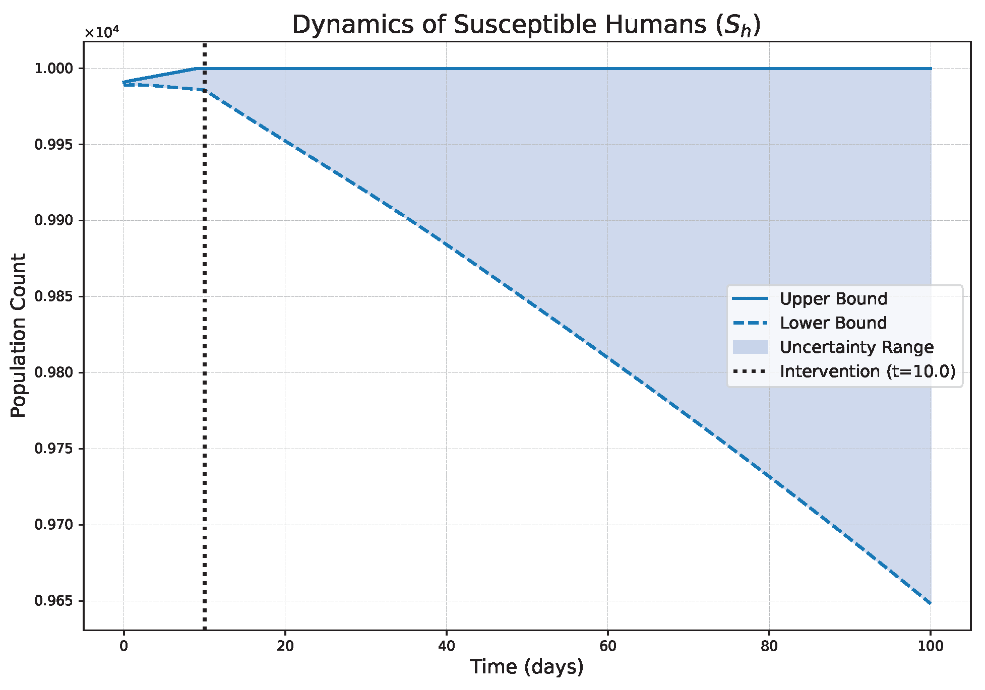
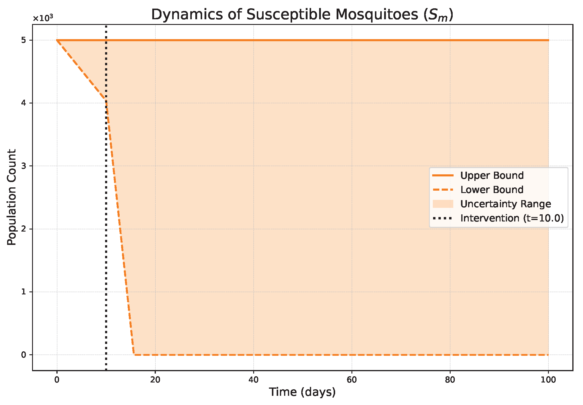
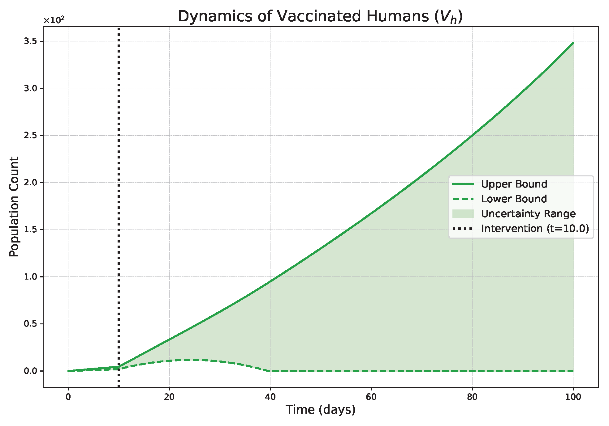
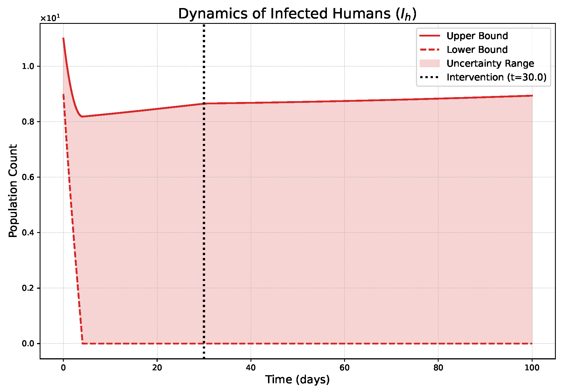
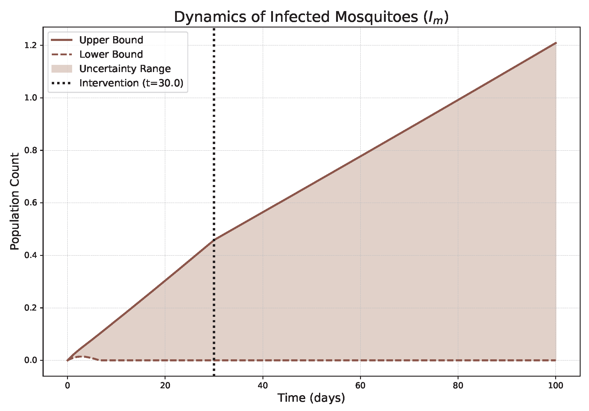
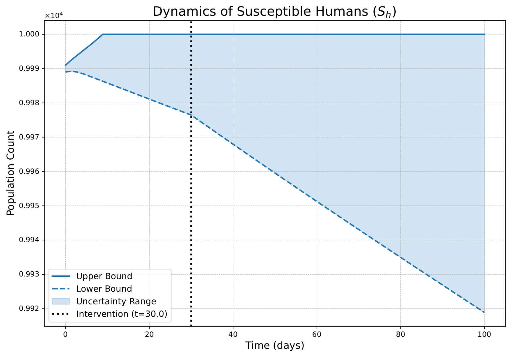
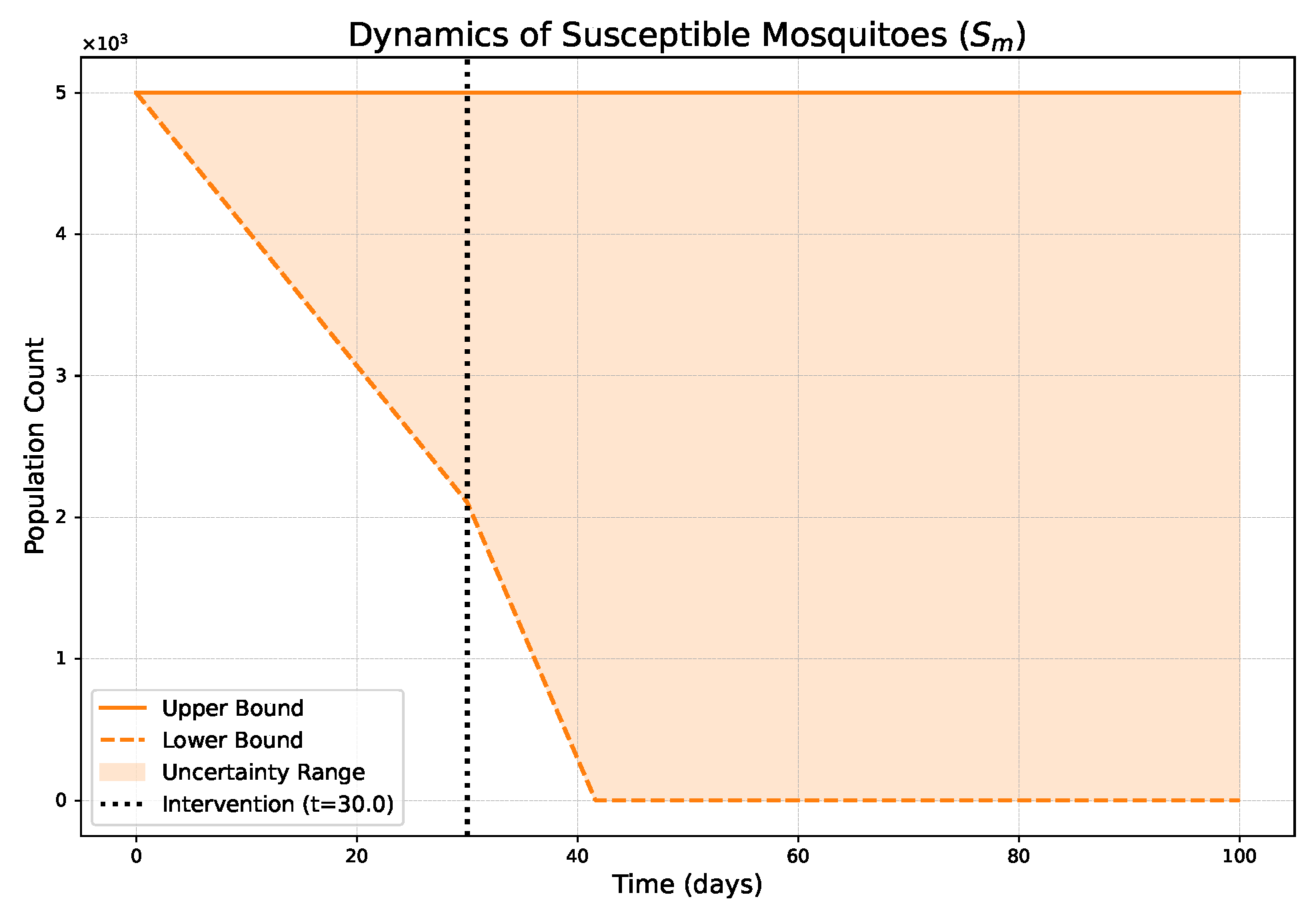
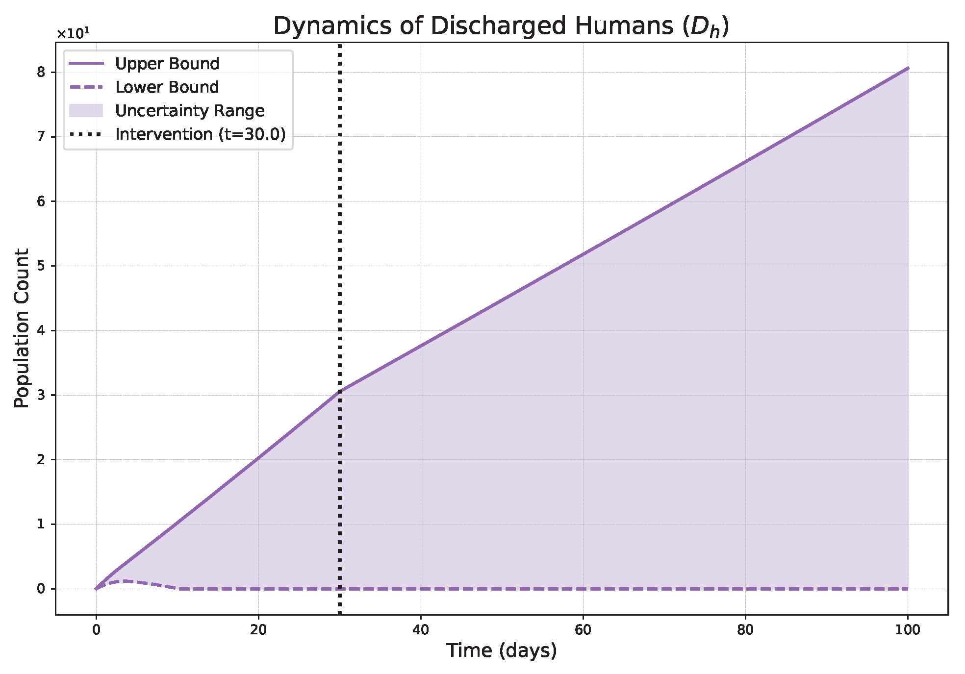
The shaded regions in Figure 1, Figure 2, Figure 3, Figure 4, Figure 5, Figure 6, Figure 7, Figure 8, Figure 9, Figure 10, Figure 11 and Figure 12 represent the fuzzy uncertainty bands. These bands are not statistical confidence intervals but rather the envelope of all possible epidemic trajectories given the specified ± 10 % uncertainty in our model parameters. The upper bound of a band for the infected compartments represents a plausible worst-case scenario, crucial for planning hospital capacity, while the lower bound provides a best-case baseline. The width of the band itself is a direct measure of the forecast’s certainty: wider bands indicate that small uncertainties in the model’s inputs lead to large variations in outcomes, signaling a less predictable system.
Case 1: With order   α = 0 . 20
The simulation results clearly demonstrate the power of the FPFD framework. In the initial phase ( t = 10 ), Figure 1, Figure 2, Figure 3, Figure 4 and Figure 5 show the fuzzy dynamics of infected humans, I ˜ h ( t ) (Figure 1); fuzzy dynamics of infected mosquitoes, I ˜ m ( t ) (Figure 2); fuzzy dynamics of susceptible humans, S ˜ h ( t ) (Figure 3); fuzzy dynamics of susceptible mosquitoes, S ˜ m ( t ) (Figure 4); fuzzy dynamics of discharged humans, D ˜ h ( t ) (Figure 5); and fuzzy dynamics of vaccinated humans, V ˜ m ( t ) (Figure 6).
Case 2: With high order   α = 0 . 95
The simulation results clearly demonstrate the power of the FPFD framework. In the initial phase ( t = 30 ), Figure 7, Figure 8, Figure 9, Figure 10, Figure 11 and Figure 12 show the fuzzy dynamics of infected humans, I ˜ h ( t ) (Figure 7); fuzzy dynamics of infected mosquitoes, I ˜ m ( t ) (Figure 8); fuzzy dynamics of susceptible humans, S ˜ h ( t ) (Figure 9); fuzzy dynamics of susceptible mosquitoes, S ˜ m ( t ) (Figure 10); fuzzy dynamics of discharged humans, D ˜ h ( t ) (Figure 11); and fuzzy dynamics of vaccinated humans, V ˜ m ( t ) (Figure 12).
The numerical simulations, presented in Figure 1, Figure 2, Figure 3, Figure 4, Figure 5, Figure 6, Figure 7, Figure 8, Figure 9, Figure 10, Figure 11 and Figure 12, provide compelling evidence of the framework’s descriptive power and yield several key conclusions:
  • The FPFD framework effectively models structural shifts in epidemic dynamics. The clear inflection points in the trajectories at the transition time t 1 demonstrate the model’s ability to switch from a memoryless (classical fuzzy) regime to a memory-dependent (ABC fuzzy fractional) regime. This allows for a more realistic representation of how interventions can fundamentally alter the course of an outbreak.
  • The fractional order α is a critical determinant of epidemic “personality”. The simulations conclusively show that α acts as a powerful modulator of system memory, with direct biological interpretations:
  • Low α (strong memory), as shown in Figure 1, Figure 2, Figure 3, Figure 4, Figure 5 and Figure 6, results in a protracted, “smoldering” epidemic. The system exhibits high inertia, where interventions are slow to take effect, and the disease persists over a long duration. The associated uncertainty bands consistently widen, signifying that long-term forecasting in such systems is inherently less certain.
  • High α (weak memory), as shown in Figure 7, Figure 8, Figure 9, Figure 10, Figure 11 and Figure 12, produces a fast-moving epidemic characterized by a sharp incidence peak, followed by a rapid response to intervention and convergence to a stable endemic equilibrium. The uncertainty remains bounded and narrow, indicating a more predictable system.
The fuzzy approach provides a quantitative tool for risk assessment. The interval-valued solutions (the shaded uncertainty bands in all figures) represent a significant advancement over deterministic, single-point forecasts. This framework provides a range of plausible outcomes, which is invaluable for public health planning. The upper bound of the infected compartments can directly inform worst-case scenario planning for hospital capacity and resource allocation, while the lower bound can help establish baselines for easing restrictions.
While the individual figures demonstrate the model’s behavior under different conditions, their collective strategic value is best understood through a synthesized summary. To this end, Table A1 has been constructed to explicitly translate our simulation findings into a practical guide for policy consideration. The value of these simulations extends beyond mathematical validation to provide a quantitative tool for public health strategy. The interval-valued solutions (the shaded uncertainty bands in all figures) represent a significant advancement over deterministic, single-point forecasts. This framework provides a range of plausible outcomes, which is invaluable for risk-based planning. For instance, the upper bound of the infected compartments can directly inform worst-case scenario planning for hospital capacity and resource allocation, while the lower bound can help establish baselines for easing restrictions. Furthermore, the model’s piecewise nature allows for the simulation of different intervention timings ( t 1 ), while the fractional order α modulates the system’s “inertia.” As shown, a low α (strong memory) results in a “smoldering” epidemic where short-term interventions are insufficient (Figure 1, Figure 2, Figure 3, Figure 4, Figure 5 and Figure 6), justifying the need for sustained policies. Conversely, a high α (weak memory) leads to a rapid response (Figure 7, Figure 8, Figure 9, Figure 10, Figure 11 and Figure 12), supporting the effectiveness of decisive, swift action.
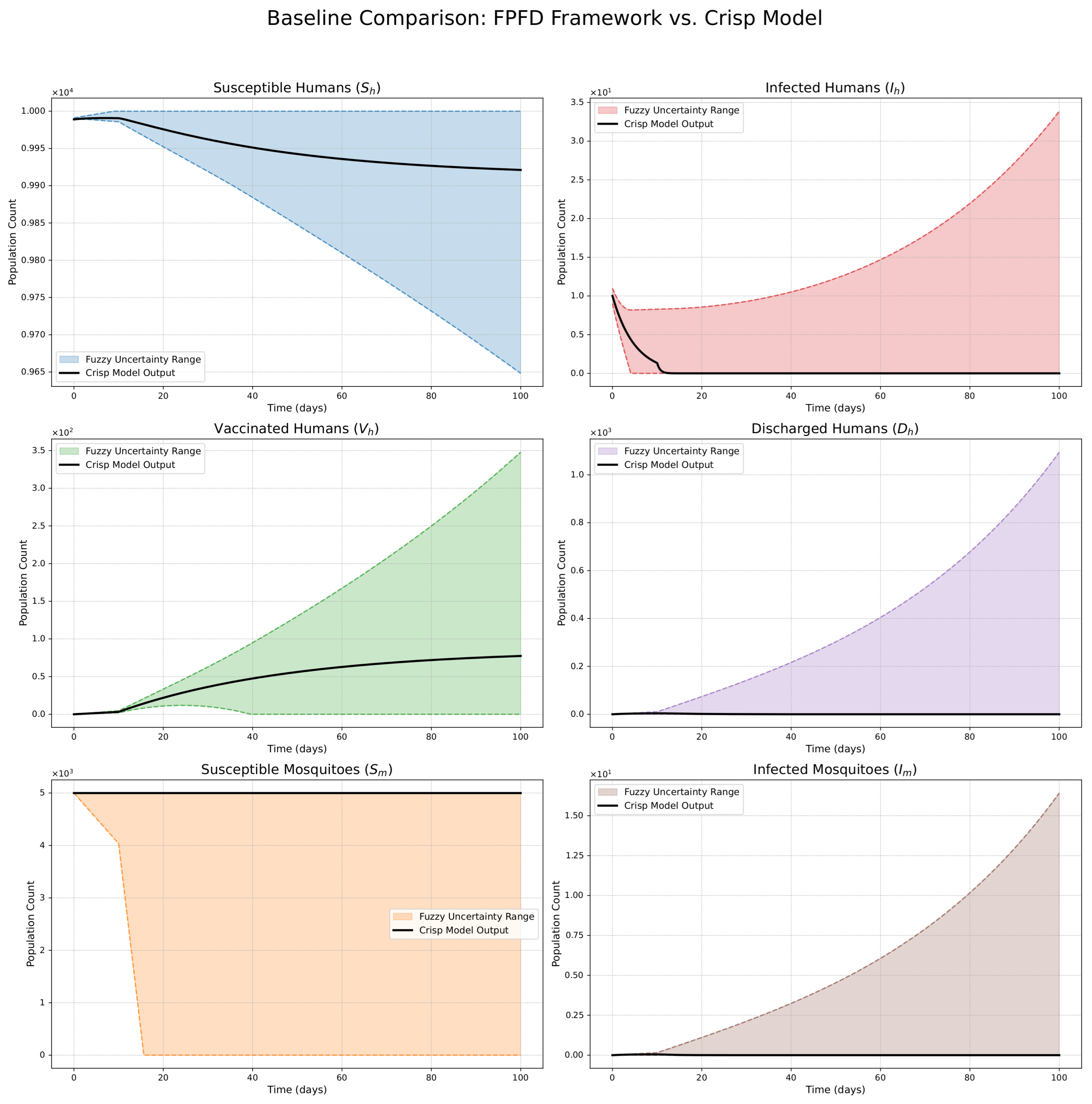
To visually underscore the primary contribution of the FPFD framework, a direct comparison against a traditional, deterministic model was performed. Figure 13 overlays the fuzzy uncertainty bands generated by our model with the single-trajectory output from a crisp (non-fuzzy) model that uses the central values of our defined parameter ranges. The crisp model’s trajectory consistently evolves along the core of the fuzzy solution, validating that our framework correctly encapsulates the deterministic dynamics as its central tendency. Most importantly, the figure illuminates what the crisp model misses: the full range of other plausible epidemic outcomes resulting from inherent parameter uncertainty. The shaded regions represent the envelope of possibilities that the FPFD framework quantifies, providing a richer and more practical forecast for strategic planning compared with the single, and potentially misleading, forecast of a deterministic model.

11. Conclusions

This paper introduced and analyzed a novel Fuzzy Piecewise Fractional Derivative (FPFD) framework for epidemiological modeling. By reformulating the Omicron–malaria co-infection model, we have created a system that captures two critical realities often overlooked in classical models: the phased nature of epidemics influenced by interventions and the inherent uncertainty in their parameters. We have rigorously established the model’s biological feasibility through positivity and boundedness proofs and confirmed its mathematical robustness via local and global stability analysis. The developed hybrid numerical scheme provides a practical tool for generating fuzzy forecasts. The simulations clearly show the model’s ability to describe a dynamic shift from a memoryless outbreak to a memory-dependent, controlled phase, all while quantifying the propagation of uncertainty. This approach represents a significant advancement, offering a more realistic and nuanced tool for understanding and managing complex infectious disease dynamics. In conclusion, the FPFD framework provides a more realistic and nuanced tool for understanding and managing complex infectious disease dynamics. Our framework simultaneously accounts for phased interventions, system memory, and parameter uncertainty. In doing so, it bridges the gap between theoretical modeling and the strategic needs of public health decision-making. While this study demonstrates the framework’s potential, we acknowledge its limitations as avenues for future work. The model relies on parameters from the literature rather than fitting them to specific surveillance data. Future research should focus on applying this framework to real-world datasets to estimate fuzzy parameters and validate its predictive capabilities. Furthermore, the fuzzy concepts employed here are part of a much broader and continually developing field. The rich algebraic theory of fuzzy mathematics offers even more sophisticated tools that could be adapted for future epidemiological models. For instance, advanced structures such as fuzzy (m,n)-filters in ordered semigroups [42], fuzzy bi-ideals in ordered semirings [43], and the integrity of m-polar fuzzy graphs [44] could potentially be used to model complex network effects, relational dynamics between population subgroups, or the robustness of transmission pathways. Furthermore, the recent application of m-polar fuzzy saturation graphs [45] and inverse graphs [46] to solve optimized allocation problems in manufacturing and robotics provides a direct analogue for future work in optimizing the distribution of limited medical resources, such as vaccines or hospital beds, during an epidemic. Exploring these more abstract fuzzy structures remains a promising avenue for future research.

Author Contributions

Conceptualization, M.S.A.; Formal analysis, M.A. and A.A.; Investigation, M.S.A.; Methodology, M.S.A., A.A.Q., and A.A.; Project administration, A.A.Q. and K.A.; Supervision, K.A.; Writing—review and editing, A.A.Q., M.A., K.A., M.H.A., and S.O.A. All authors have read and agreed to the published version of the manuscript.

Funding

This work was supported and funded by the Deanship of Scientific Research at Imam Mohammad Ibn Saud Islamic University (IMSIU) (grant number IMSIU-DDRSP2501).

Data Availability Statement

The paper contains all data that were either created or analyzed throughout the course of this research.

Conflicts of Interest

The authors declare that they have no conflicts of interest.

Appendix A

Definition A1.
A fuzzy number u ˜ is a mapping u ˜ : R [ 0 , 1 ] that is normal, fuzzy convex, upper semi-continuous, and has a compact support. Its parametric, or r-level, form is given by:
[ u ˜ ] r = [ u ̲ ( r ) , u ¯ ( r ) ] , r [ 0 , 1 ] ,
where u ̲ ( r ) and u ¯ ( r ) are the lower and upper bounds of the interval, respectively.
The dynamics of fuzzy functions often involve subtraction, which requires a generalized approach. The generalized Hukuhara difference is defined as the following definition.
Definition A2.
Let u ˜ and v ˜ be two fuzzy numbers. The generalized Hukhara difference of u ˜ and v ˜ is defined as follows:
u ˜ g H v ˜ = w ˜ ( i ) u ˜ = v ˜ w ˜ , ( i i ) v ˜ = u ˜ 1 w ˜ ,
and
u ˜ g H v ˜ = min u ̲ ( r ) v ̲ ( r ) , u ¯ ( r ) v ¯ ( r ) , max u ̲ ( r ) v ̲ ( r ) , u ¯ ( r ) v ¯ ( r ) .
Definition A3
(Fuzzy Classical Derivative). The gH-derivative of a fuzzy function y ˜ ( t ) is denoted D 1 C [ y ˜ ( t ) ] and defined as
D 1 C [ y ˜ ( t ) ] = lim h 0 + y ˜ ( t + h ) g H y ˜ ( t ) h .
The existence of this limit leads to two cases. Case (i) corresponds to systems where the uncertainty interval is non-decreasing, while Case (ii) allows for the interval width to decrease, modeling convergence towards a crisp state.
Definition A4
(Fuzzy ABC Derivative). To incorporate memory effects, we use the fuzzy Atangana–Baleanu–Caputo (ABC) derivative. For α ( 0 , 1 ] , the fuzzy ABC derivative of a function y ˜ ( t ) is
D t α ABC [ y ˜ ( t ) ] = B ( α ) 1 α 0 t E α α 1 α ( t τ ) α D 1 C [ y ˜ ( τ ) ] d τ ,
where B ( α ) is a normalization constant. The significance of the ABC derivative lies in its non-singular Mittag-Leffler kernel, E α . This kernel is particularly adept at modeling complex biological memory effects due to its ability to interpolate between power-law (characteristic of long-term memory) and exponential-decay (characteristic of short-term memory) behaviors, thereby capturing a wide range of hereditary properties in the system.
Definition A5
(Hausdorff Metric and its Properties). The space of fuzzy numbers R F can be equipped with the Hausdorff metric, d H , which measures the distance between two fuzzy numbers u ˜ and v ˜ . Based on their r-level representations, it is defined as
d H ( u ˜ , v ˜ ) = sup r [ 0 , 1 ] max | u ̲ ( r ) v ̲ ( r ) | , | u ¯ ( r ) v ¯ ( r ) | .
The space ( R F , d H ) is a complete metric space. The metric satisfies the following properties for any u ˜ , v ˜ , w ˜ R F and scalar k R :
1. 
d H ( u ˜ , v ˜ ) 0 (Non-negativity).
2. 
d H ( u ˜ , v ˜ ) = 0 u ˜ = v ˜ (Identity).
3. 
d H ( u ˜ , v ˜ ) = d H ( v ˜ , u ˜ ) (Symmetry).
4. 
d H ( u ˜ w ˜ , v ˜ w ˜ ) = d H ( u ˜ , v ˜ ) (Property of addition).
5. 
d H ( k u ˜ , k v ˜ ) = | k | d H ( u ˜ , v ˜ ) (Property of scalar multiplication).
6. 
d H ( u ˜ v ˜ , w ˜ z ˜ ) d H ( u ˜ , w ˜ ) + d H ( v ˜ , z ˜ ) (Triangle inequality for addition).

Appendix B

Table A1. Interpretation of simulation figures for public health policy.
Model FeatureSimulation Result (Observed in Figures)Real-Life Policy Implication
Piecewise NatureDynamics exhibit a clear structural shift at t 1 : a gradual trend reversal (Figure 1, Figure 2, Figure 3, Figure 4, Figure 5 and Figure 6) vs. rapid convergence to a new equilibrium (Figure 7, Figure 8, Figure 9, Figure 10, Figure 11 and Figure 12).Context-Dependent Strategy: Allows for testing how policy timing and type perform in different dynamic contexts (e.g., slow vs. fast-burning outbreaks).
Fuzzy Uncertainty BandsThe uncertainty bands quantify outcome variability, widening with strong memory (Figure 1) but stabilizing with weak memory (Figure 7).Enable Risk-Based Planning: The upper bound informs worst-case scenarios (hospital capacity). The band’s width indicates forecast confidence, guiding the need for adaptive vs. fixed strategies.
Strong Memory (Low α = 0.20)High system inertia is shown; an early intervention at t 1 = 10 fails to halt momentum, leading to a slow, accelerating resurgence post-intervention (Figure 1).Justify Sustained Policies: Demonstrates that short-term actions are insufficient for diseases with high inertia (e.g., environmental persistence), necessitating long-term, continuous strategies.
Weak Memory (High α = 0 . 95 )The system shows a rapid response; intervention at t 1 = 30 halts the outbreak and induces a stable, low-level endemic state (Figure 7).Support Rapid, Decisive Action: Provides evidence that swift interventions are highly effective for controlling fast-moving epidemics and establishing predictable, long-term outcomes.

References

  1. Brauer, F.; Castillo-Chavez, C.; Feng, Z. Mathematical Models in Epidemiology; Springer: New York, NY, USA, 2019; Volume 32. [Google Scholar]
  2. Allen, L.J.; Brauer, F.; Van den Driessche, P.; Wu, J. Mathematical Epidemiology; Springer: Berlin/Heidelberg, Germany, 2008; Volume 1945. [Google Scholar]
  3. Siettos, C.I.; Russo, L. Mathematical modeling of infectious disease dynamics. Virulence 2013, 4, 295–306. [Google Scholar] [CrossRef] [PubMed]
  4. Diekmann, O.; Heesterbeek, J.A.P. Mathematical Epidemiology of Infectious Diseases: Model Building, Analysis and Interpretation; John Wiley Sons: Hoboken, NJ, USA, 2000; Volume 5. [Google Scholar]
  5. Martcheva, M. An Introduction to Mathematical Epidemiology; Springer: New York, NY, USA, 2015; Volume 61, pp. 9–31. [Google Scholar]
  6. Ortiz-Barrios, M.; Petrillo, A.; Arias-Fonseca, S.; McClean, S.; de Felice, F.; Nugent, C.; Uribe-López, S.A. An AI-based multiphase framework for improving the mechanical ventilation availability in emergency departments during respiratory disease seasons: A case study. Int. J. Emerg. Med. 2024, 17, 45. [Google Scholar] [CrossRef] [PubMed]
  7. Barmpounakis, P.; Demiris, N. Multiphasic stochastic epidemic models. J. R. Stat. Soc. Ser. C Appl. Stat. 2025, 74, 491–505. [Google Scholar] [CrossRef]
  8. Vieira, L.C.; Costa, R.S.; Valério, D. An overview of mathematical modelling in cancer research: Fractional calculus as modelling tool. Fractal Fract. 2023, 7, 595. [Google Scholar] [CrossRef]
  9. Wang, J. Mathematical models for cholera dynamics—A review. Microorganisms 2022, 10, 2358. [Google Scholar] [CrossRef]
  10. Bendib, I.; Hammad, M.M.A.; Ouannas, A.; Grassi, G. The Discrete SIR Epidemic Reaction–Diffusion Model: Finite-Time Stability and Numerical Simulations. Comput. Math. Methods 2025, 2025, 9597093. [Google Scholar] [CrossRef]
  11. Atangana, A.; Araz, S.İ. New concept in calculus: Piecewise differential and integral operators. Chaos Solitons Fractals 2021, 145, 110638. [Google Scholar] [CrossRef]
  12. Arık, İ.A.; Araz, S.İ. Crossover behaviors via piecewise concept: A model of tumor growth and its response to radiotherapy. Results Phys. 2022, 41, 105894. [Google Scholar] [CrossRef]
  13. Naik, P.A.; Farman, M.; Jamil, K.; Nisar, K.S.; Hashmi, M.A.; Huang, Z. Modeling and analysis using piecewise hybrid fractional operator in time scale measure for ebola virus epidemics under Mittag–Leffler kernel. Sci. Rep. 2024, 14, 24963. [Google Scholar] [CrossRef]
  14. Aldwoah, K.A.; Almalahi, M.A.; Shah, K.; Awadalla, M.; Egami, R.H. Dynamics analysis of dengue fever model with harmonic mean type under fractal-fractional derivative. AIMS Math. 2024, 9, 13894–13926. [Google Scholar] [CrossRef]
  15. Alraqad, T.; Almalahi, M.A.; Mohammed, N.; Alahmade, A.; Aldwoah, K.A.; Saber, H. Modeling Ebola dynamics with a Φ-piecewise hybrid fractional derivative approach. Fractal Fract. 2024, 8, 596. [Google Scholar] [CrossRef]
  16. Shah, K.; Khan, A.; Abdalla, B.; Abdeljawad, T.; Khan, K.A. A mathematical model for Nipah virus disease by using piecewise fractional order Caputo derivative. Fractals 2024, 32, 2440013. [Google Scholar] [CrossRef]
  17. Saleem, M.U.; Farman, M.; Nisar, K.S.; Ahmad, A.; Munir, Z.; Hincal, E. Investigation and application of a classical piecewise hybrid with a fractional derivative for the epidemic model: Dynamical transmission and modeling. PLoS ONE 2024, 19, e0307732. [Google Scholar] [CrossRef]
  18. Saber, H.; Almalahi, M.A.; Albala, H.; Aldwoah, K.; Alsulami, A.; Shah, K.; Moumen, A. Investigating a nonlinear fractional evolution control model using W-piecewise hybrid derivatives: An application of a breast cancer model. Fractal Fract. 2024, 8, 735. [Google Scholar]
  19. Zadeh, L.A. Fuzzy sets. Inf. Control 1965, 8, 338–353. [Google Scholar] [CrossRef]
  20. Vasudevan, A.; Yogeesh, N.; Mohammad, S.I.; Raja, N.; Girija, D.K.; Rashmi, M.; Abu-Shareha, A.A.; Alshurideh, M.T. Unlocking Insights of Fuzzy Mathematics for Enhanced Predictive Modelling. Appl. Math. 2025, 19, 49–60. [Google Scholar]
  21. Bryniarska, A. Mathematical models of diagnostic information granules generated by scaling intuitionistic fuzzy sets. Appl. Sci. 2022, 12, 2597. [Google Scholar] [CrossRef]
  22. Bera, S.; Khajanchi, S.; Roy, T.K. Stability analysis of fuzzy HTLV-I infection model: A dynamic approach. J. Appl. Math. Comput. 2023, 69, 171–199. [Google Scholar] [CrossRef]
  23. Ejegwa, P.A.; Muhiuddin, G.; Algehyne, E.A.; Agbetayo, J.M.; Al-Kadi, D. An Enhanced Fermatean Fuzzy Composition Relation Based on a Maximum-Average Approach and Its Application in Diagnostic Analysis. J. Math. 2022, 2022, 1786221. [Google Scholar]
  24. Gul, R.; Ayub, S.; Shabir, M.; Hummdi, A.Y.; Aljaedi, A.; Bassfar, Z. A novel approach for fuzzification of rough sets based on fuzzy preference relation: Properties and application to medicine selection problem. IEEE Access 2024, 12, 67681–67703. [Google Scholar] [CrossRef]
  25. Ayub, S.; Gul, R.; Shabir, M.; Hummdi, A.Y.; Aljaedi, A.; Bassfar, Z. A novel approach to roughness of linear diophantine fuzzy sets by fuzzy relations and its application toward multi-criteria group decision-making. IEEE Access 2024, 12, 53549–53564. [Google Scholar] [CrossRef]
  26. Areshi, M.; El-Tantawy, S.A.; Alotaibi, B.M.; Zaland, S. Study of Fuzzy Fractional Third-Order Dispersive KdV Equation in a Plasma under Atangana-Baleanu Derivative. J. Funct. Spaces 2022, 2022, 7922001. [Google Scholar] [CrossRef]
  27. Boulaaras, S.; Rehman, Z.U.; Abdullah, F.A.; Jan, R.; Abdalla, M.; Jan, A. Coronavirus dynamics, infections and preventive interventions using fractional-calculus analysis. AIMS Math. 2023, 8, 8680–8701. [Google Scholar] [CrossRef]
  28. Aldwoah, K.A.; Almalahi, M.A.; Abdulwasaa, M.A.; Shah, K.; Kawale, S.V.; Awadalla, M.; Alahmadi, J. Mathematical analysis and numerical simulations of the piecewise dynamics model of Malaria transmission: A case study in Yemen. AIMS Math. 2024, 9, 4376–4408. [Google Scholar] [CrossRef]
  29. Subramanian, S.; Kumaran, A.; Ravichandran, S.; Venugopal, P.; Dhahri, S.; Ramasamy, K. Fuzzy fractional Caputo derivative of susceptible-infectious-removed epidemic model for childhood diseases. Mathematics 2024, 12, 466. [Google Scholar] [CrossRef]
  30. Qayyum, M.; Fatima, Q.; Akgül, A.; Hassani, M.K. Modeling and analysis of dengue transmission in fuzzy-fractional framework: A hybrid residual power series approach. Sci. Rep. 2024, 14, 30706. [Google Scholar] [CrossRef] [PubMed]
  31. Gassem, F.; Qurtam, A.A.; Almalahi, M.; Rabih, M.; Aldwoah, K.; El-Sayed, A.; Hassan, E.I. Exploring SEIR Influenza Epidemic Model via Fuzzy ABC Fractional Derivatives with Crowley–Martin Incidence Rate. Fractal Fract. 2025, 9, 402. [Google Scholar] [CrossRef]
  32. ul Rehman, A.; Singh, R.; Sharma, N.; Singh, J.; Baleanu, D. Optimal solution and sensitivity analysis of fractional-order mathematical modeling of the omicron variant and malaria co-infection. Alex. Eng. J. 2025, 116, 364–373. [Google Scholar] [CrossRef]
  33. Lefevr, N.; Kanavos, A.; Gerogiannis, V.C.; Iliadis, L.; Pintelas, P. Employing fuzzy logic to analyze the structure of complex biological and epidemic spreading models. Mathematics 2021, 9, 977. [Google Scholar] [CrossRef]
  34. Thangaraj, C.; Easwaramoorthy, D.; Muhiuddin, G.; Selmi, B.; Kulish, V. Fractal based automatic detection of complexity in COVID-19 X-ray images. Expert Syst. 2025, 42, e13497. [Google Scholar] [CrossRef]
  35. Zadeh, L.A. Fuzzy Sets A Basis A Theory possibility. Fuzzy Sets Syst. 1978, 1, 3–28. [Google Scholar] [CrossRef]
  36. Bede, B.; Stefanini, L. Generalized differentiability of fuzzy-valued functions. Fuzzy Sets Syst. 2013, 230, 119–141. [Google Scholar] [CrossRef]
  37. Allahviranloo, T.; Salahshour, S.; Abbasbandy, S. Explicit solutions of fractional differential equations with uncertainty. Soft Comput. 2012, 16, 297–302. [Google Scholar] [CrossRef]
  38. Allahviranloo, T.; Ghanbari, B. On the fuzzy fractional differential equation with interval Atangana–Baleanu fractional derivative approach. Chaos Solitons Fractals 2020, 130, 109397. [Google Scholar] [CrossRef]
  39. Cortez, M.V.; Althobaiti, A.; Aljohani, A.F.; Althobaiti, S. Generalized Fuzzy-Valued Convexity with Ostrowski’s, and Hermite-Hadamard Type Inequalities over Inclusion Relations and Their Applications. Axioms 2024, 13, 471. [Google Scholar] [CrossRef]
  40. Altaweel, N.H.; Rashid, M.H.; Albalawi, O.; Alshehri, M.G.; Eljaneid, N.H.; Albalawi, R. On the Ideal Convergent Sequences in Fuzzy Normed Space. Symmetry 2023, 15, 936. [Google Scholar] [CrossRef]
  41. van den Driessche, P.; Watmough, J. Reproduction numbers and sub-threshold endemic equilibria for compartmental models of disease transmission. Math. Biosci. 2002, 180, 29–48. [Google Scholar] [CrossRef]
  42. Mahboob, A.; Al-Tahan, M.; Muhiuddin, G. Fuzzy (m, n)-filters based on fuzzy points in ordered semigroups. Comput. Appl. Math. 2023, 42, 245. [Google Scholar] [CrossRef]
  43. Muhiuddin, G.; Abughazalah, N.; Mahboob, A.; Al-Kadi, D. A Novel study of fuzzy bi-ideals in ordered semirings. Axioms 2023, 12, 626. [Google Scholar] [CrossRef]
  44. Muhiuddin, G.; Mahapatra, T.; Pal, M.; Alshahrani, O.; Mahboob, A. Integrity on m-polar fuzzy graphs and its application. Mathematics 2023, 11, 1398. [Google Scholar] [CrossRef]
  45. Alanazi, A.M.; Muhiuddin, G.; Alenazi, B.M.; Mahapatra, T.; Pal, M. Utilizing m-Polar Fuzzy Saturation Graphs for Optimized Allocation Problem Solutions. Mathematics 2023, 11, 4136. [Google Scholar] [CrossRef]
  46. Alanazi, A.M.; Muhiuddin, G.; Mahapatra, T.; Bassfar, Z.; Pal, M. Inverse Graphs in m-Polar Fuzzy Environments and Their Application in Robotics Manufacturing Allocation Problems with New Techniques of Resolvability. Symmetry 2023, 15, 1387. [Google Scholar] [CrossRef]
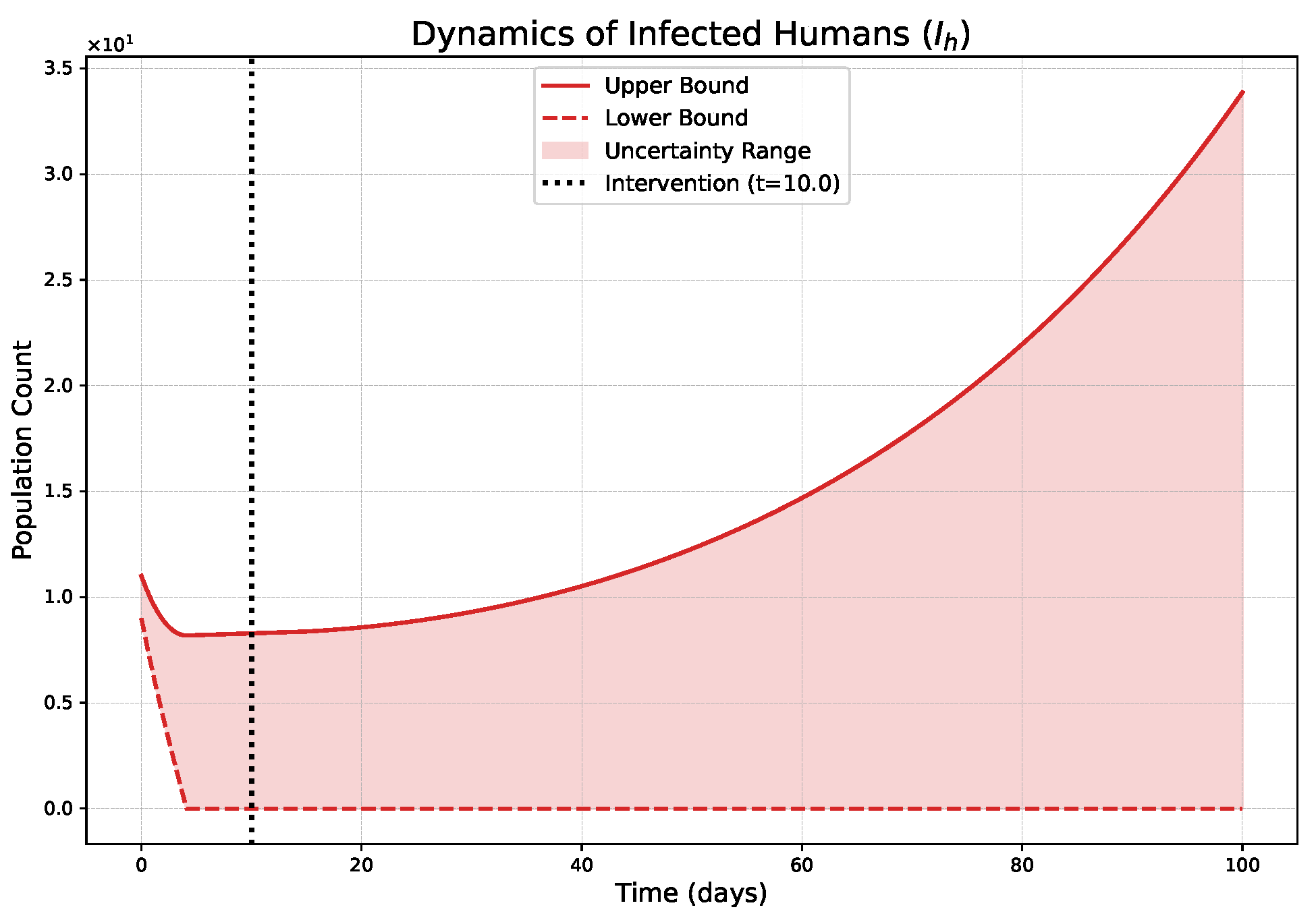
Figure 1. Fuzzy dynamics of infected humans, I ˜ h ( t ) with order α = 0.20 . The shaded region represents the fuzzy uncertainty band, showing the range of all possible outcomes given the ± 10 % parameter uncertainty. The dashed vertical line indicates the intervention time at t 1 = 10 .
Fractalfract 09 00643 g001
Figure 2. Fuzzy dynamics of infected mosquitoes, I ˜ m ( t ) with order α = 0.20 . The shaded region represents the fuzzy uncertainty band, showing the range of all possible outcomes given the ± 10 % parameter uncertainty. The dashed vertical line indicates the intervention time at t 1 = 10 .
Fractalfract 09 00643 g002
Figure 3. Fuzzy dynamics of susceptible humans, S ˜ h ( t ) with order α = 0.20 . The shaded region represents the fuzzy uncertainty band, showing the range of all possible outcomes given the ± 10 % parameter uncertainty. The dashed vertical line indicates the intervention time at t 1 = 10 .
Fractalfract 09 00643 g003
Figure 4. Fuzzy dynamics of susceptible mosquitoes, S ˜ m ( t ) with order α = 0.20 . The shaded region represents the fuzzy uncertainty band, showing the range of all possible outcomes given the ± 10 % parameter uncertainty. The dashed vertical line indicates the intervention time at t 1 = 10 .
Fractalfract 09 00643 g004
Figure 5. Fuzzy dynamics of discharged humans, D ˜ h ( t ) with order α = 0.20 . The shaded region represents the fuzzy uncertainty band, showing the range of all possible outcomes given the ± 10 % parameter uncertainty. The dashed vertical line indicates the intervention time at t 1 = 10 .
Fractalfract 09 00643 g005
Figure 6. Fuzzy dynamics of vaccinated humans, V ˜ h ( t ) with order α = 0.20 . The shaded region represents the fuzzy uncertainty band, showing the range of all possible outcomes given the ± 10 % parameter uncertainty. The dashed vertical line indicates the intervention time at t 1 = 10 .
Fractalfract 09 00643 g006
Figure 7. Fuzzy dynamics of infected humans, I ˜ h ( t ) with order α = 0.95 . The shaded region represents the fuzzy uncertainty band, showing the range of all possible outcomes given the ± 10 % parameter uncertainty. The dashed vertical line indicates the intervention time at t 1 = 30 .
Fractalfract 09 00643 g007
Figure 8. Fuzzy dynamics of infected mosquitoes, I ˜ m ( t ) with order α = 0.95 . The shaded region represents the fuzzy uncertainty band, showing the range of all possible outcomes given the ± 10 % parameter uncertainty. The dashed vertical line indicates the intervention time at t 1 = 30 .
Fractalfract 09 00643 g008
Figure 9. Fuzzy dynamics of susceptible humans, S ˜ h ( t ) with order α = 0.95 . The shaded region represents the fuzzy uncertainty band, showing the range of all possible outcomes given the ± 10 % parameter uncertainty. The dashed vertical line indicates the intervention time at t 1 = 30 .
Fractalfract 09 00643 g009
Figure 10. Fuzzy dynamics of susceptible mosquitoes, S ˜ m ( t ) with order α = 0.95 . The shaded region represents the fuzzy uncertainty band, showing the range of all possible outcomes given the ± 10 % parameter uncertainty. The dashed vertical line indicates the intervention time at t 1 = 30 .
Fractalfract 09 00643 g010
Figure 11. Fuzzy dynamics of discharged humans, D ˜ h ( t ) with order α = 0.95 . The shaded region represents the fuzzy uncertainty band, showing the range of all possible outcomes given the ± 10 % parameter uncertainty. The dashed vertical line indicates the intervention time at t 1 = 30 .
Fractalfract 09 00643 g011
Figure 12. Fuzzy dynamics of vaccinated humans, V ˜ h ( t ) with order α = 0.95 . The shaded region represents the fuzzy uncertainty band, showing the range of all possible outcomes given the ± 10 % parameter uncertainty. The dashed vertical line indicates the intervention time at t 1 = 30 .
Fractalfract 09 00643 g012
Figure 13. Baseline comparison: FPFD framework vs. crisp model.
Fractalfract 09 00643 g013
Table 1. Parameters of the Omicron–malaria co-infection model.
ParameterBiological MeaningValue/RangeUnit
Human Population Dynamics
Ω 1 Recruitment rate of the human population.0.05day−1
d h Natural death rate of humans.0.039day−1
ω h Disease-induced death rate for Omicron-infected humans.0.3day−1
α v a c Proportion of new arrivals who are vaccinated against Omicron.0.8Dimensionless
Disease Transmission Dynamics
β h Transmission rate of Omicron from infected humans to susceptible humans.0.5(person·day)−1
β m Transmission rate of Malaria from infected humans to susceptible mosquitoes.0.85(mosquito·day)−1
Disease Progression and Recovery (Omicron)
γ h Recovery rate of Omicron-infected humans.0.05day−1
η Discharge rate of Omicron-infected humans (moving to the D h class).0.6day−1
ρ Rate of waning immunity from Omicron vaccination.0.07day−1
b h Recovery rate for discharged individuals.0.17Dimensionless
m h Disease-induced death rate for discharged individuals.0.25Dimensionless
Mosquito (Vector) Population Dynamics
Ω 2 Recruitment rate of the vector population.4.0day−1
d m Natural death rate of mosquitoes.0.4day−1
Fuzzy Piecewise Operator Parameters
t 1 Central time of intervention (transition from classical to fractional).10, 30days
α Fractional order of the ABC derivative (controls system memory).0.2–0.95Dimensionless
Disclaimer/Publisher’s Note: The statements, opinions and data contained in all publications are solely those of the individual author(s) and contributor(s) and not of MDPI and/or the editor(s). MDPI and/or the editor(s) disclaim responsibility for any injury to people or property resulting from any ideas, methods, instructions or products referred to in the content.