Article

Stylized Facts of High-Frequency Bitcoin Time Series

by
Yaoyue Tang
1,
Karina Arias-Calluari
2,
Morteza Nattagh Najafi
3,
Michael S. Harré
1 and
Fernando Alonso-Marroquin
4,*
1
Modelling and Simulation Research Group, The University of Sydney, Sydney, NSW 2006, Australia
2
School of Mathematics and Statistics, The University of Sydney, Sydney, NSW 2006, Australia
3
Department of Physics, University of Mohaghegh Ardabili, Ardabil P.O. Box 179, Iran
4
Center for Integrative Petroleum Research, King Fahd University of Petroleum and Minerals, Dhahran 31261, Saudi Arabia
*
Author to whom correspondence should be addressed.
Fractal Fract. 2025, 9(10), 635; https://doi.org/10.3390/fractalfract9100635
Submission received: 1 September 2025 / Revised: 20 September 2025 / Accepted: 24 September 2025 / Published: 29 September 2025
(This article belongs to the Special Issue Fractional Porous Medium Type and Related Equations)

Abstract

This paper analyzes high-frequency intraday Bitcoin data from 2019 to 2022. The Bitcoin market index exhibits two distinct periods, characterized by abrupt volatility shifts. Bitcoin returns can be described by anomalous diffusion processes, transitioning from subdiffusion for short intervals to weak superdiffusion at longer intervals. Heavy tails are captured well by q-Gaussian distributions, and the autocorrelation of absolute returns shows power law behavior. Both periods display multifractality, with Hurst exponents shifting toward 0.5 over time, indicating increased market efficiency. The time evolution of the empirical PDF of price return allows us to connect these stylized facts to the mathematical framework of multifractals and locally fractional porous medium equations.

1. Introduction

Fractals [1] and fractional calculus [2] provide powerful frameworks for analyzing complex, irregular, and scale-invariant systems. Their mathematical structures and anomalous scaling properties appear naturally in a wide range of phenomena, including price dynamics in financial markets [3]. The irregular fluctuations and persistent volatility observed in Bitcoin and other cryptocurrencies align with the traits of fractal geometry, such as self-similarity, heavy tails, and long-term memory effects [4]. Fractional calculus, in turn, offers a versatile extension of classical calculus, enabling models that capture memory effects, which are essential for describing market processes that persist far from statistic equilibrium [5].
Although cryptocurrencies have emerged as decentralized digital assets with disruptive potential [6], their value dynamics cannot be fully understood within the conventional frameworks of classical finance. Bitcoin, introduced by Nakamoto in 2008 [7], has become a paradigmatic example of a system where nonlinearity, unpredictability, and fractal properties coexist. By 2025, Bitcoin’s market capitalization had surpassed a trillion dollars, maintaining nearly half of the total crypto market share [8]. Its volatility and sensitivity to global conditions make it a prime candidate for analysis through the lens of fractal time series and fractional stochastic models.
Instead of focusing exclusively on traditional economic correlations, our work emphasizes the robust patterns and fractal structures that underlie Bitcoin’s price fluctuations. Previous studies in econophysics highlight the fact that, beyond market efficiency, crypto-assets exhibit stylized facts such as fat-tailed distributions [9], volatility clustering [10], and anomalous diffusion [11]. Fractional differential equations provide a natural mathematical toolkit to capture these features and extend beyond conventional stochastic models. Here, we analyze intraday BTC/USD exchange data (2018–2022) at a 10 min frequency, with the aim of unveiling fractal properties and time-scale-dependent structures. Our motivation lies in comparing these findings with established stylized facts from stock markets, thus bridging the fractal and fractional frameworks with the dynamics of the cryptocurrency.
Recent work consistently finds multifractality in Bitcoin returns and shows that its strength varies over time. Early evidence using multifractal detrending fluctuation analysis (MF-DFA) on 1 min data documented fat tails and multifractal scaling, with sources traced to both long-range correlations and heavy-tailed marginals [4]. Follow-up studies report time-varying multifractality and links to market efficiency: for example, rolling-window MF-DFA detects were found to change the multifractal degree and asymmetric volatility across regimes [12]. Other analyses show Bitcoin’s multifractal spectrum tightening or loosening around shocks and across horizons (time scales), sometimes strengthening at short horizons after COVID-19 while weakening at longer ones [13]. A dedicated MF-DFA study focused on efficiency argues that Bitcoin retains long memory and predictable structure in specific windows [14], while broader comparative work (MF-DFA with complementary entropy measures) tends to rank Bitcoin as more complex than major foreign exchanges or commodity markets, consistent with richer nonlinear correlations in high-frequency returns [15]. Overall, the literature supports viewing Bitcoin as a multifractal, regime-dependent process rather than viewing it as monofractal, which aligns well with fractal and fractional modeling frameworks. MF-DFA has been effective in exposing long-term memory and multifractal properties in financial returns, highlighting structural inefficiencies and regime shifts. However, translating these empirical findings into a formal framework based on stochastic differential equations and partial differential equations for probability of returns is necessary to enhance predictive capabilities and integrate them into stochastic market models.
The paper is organized as follows. Section 2 recalls well-known stylized facts and their connection with fractal geometry and fractional processes. Section 3 introduces the governing equations that include fractional calculus approaches. Section 4 provides a detailed fractal and fractional analysis of Bitcoin time series in different volatility regimes. In Section 5, we summarize our findings and compare them with S&P500 price return; in Section 6, we discuss the implications for future research in fractal-based models for digital assets.

2. Stylized Facts of Financial Markets

Stylized facts are persistent statistical features of markets, originally introduced in macroeconomics [16] and widely studied in finance [17]. They include fat-tailed return distributions, short-memory in raw returns, volatility clustering, fractality, and anomalous diffusion [18]. Cryptocurrencies show the same features [19,20].
  • Fat tails: Returns deviate from Gaussian and follow heavy-tailed laws [9,21]. A self-similar PDF is P ( x , t ) t H F ( x t H ) . Classical choices for F ( x ) are as follows. Lévy stable L α (x) with α = 1 / H [22,23,24]; q-Gaussian g q ( x ) , where q is given by the hyperscaling relation α = ( 3 q ) / ξ [25,26,27]; and porous media solutions with variable α ( t ) [3,5].
  • Autocorrelation: The autocorrelation function of returns A C F ( τ ) decays rapidly so that it is integrable; thus, the integrated correlation time τ c = A C F ( 0 ) 1 0 A C F ( τ ) d τ is finite [28,29,30]. This finite memory is consistent with the market efficiency [31].
  • Volatility clustering: Large fluctuations follow further large fluctuations [21], implying long memory in σ 2 ( t ) and motivating stochastic and fractional volatility models [17,32,33,34].
  • Fractality: A fractal time series has dimension D f = 2 H [35] and scaling of price return x and time t by x 2 t H . Here, x is a stochastic variable with time-dependent probability P ( x , t ) . Techniques such as DFA and MF-DFA estimate H and multifractal spectra [36,37]. Fractality is documented across many markets [10,37,38,39,40,41].
  • Anomalous diffusion: Beyond Brownian motion [42,43], markets exhibit x 2 ( t ) t 2 H with H 1 / 2 and P m a x ( t ) P ( 0 , t ) t 1 / α ( t ) [27,44]. Here, α = 2 is normal diffusion, α < 2 is superdiffusion, α > 2 is subdiffusion, with H = 1 / α ( t ) [3,34]. The Borland stochastic motion provides pathways to understand these effects [25].
We test these mathematical properties for Bitcoin and compare them with conventional markets using a fractional porous media model, as outlined in the next section.

3. Mathematical Framework

A probabilistic route to model price returns is to track the time evolution of their probability density function (PDF) via the Fokker–Planck Equation (FPE). We employ a nonlinear porous media equation FPE that admits q-Gaussian solutions and their fractional counterparts (via time stretching and the local Katugampola operator) to capture the empirical hyperscaling relation of stock markets.
  • Definitions and notation: Let I ( t ) be a market index. The simple price return from t 0 to t 0 + t is
    S ( t , t 0 ) = I ( t 0 + t ) I ( t 0 ) .
    In predictive models, t 0 is the current time and t > t 0 is the time where the price return X t 0 ( t ) is estimated. To simplify the notation, we assume t 0 = 0 . We work with detrended returns. Here, a deterministic trend means a smooth, low-frequency component (e.g., a moving-average) removed before analysis; the remaining stochastic noises are the zero-mean fluctuations captured by the stochastic dynamics introduced below. We therefore do not define separate variables for trend and noise. Define the simple price return as
    X t S ( t , 0 ) = I ( t ) I ( 0 ) ,
    where we take t 0 = 0 in Equation (1).
  • Stochastic dynamics and FPE. The model X t by the Itô SDE
    d X t = μ ( X t , t ) d t + σ ( X t , t ) d W t ,
    with W t a Wiener process. The PDF P ( x , t ) satisfies the Itô FPE
    t P = x ( μ P ) + 1 2 x 2 ( σ 2 P ) .
    For detrended returns ( μ 0 ),
    t P ( x , t ) = 1 2 x 2 σ 2 ( x , t ) P ( x , t ) .
  • Nonlinear diffusion (q-Gaussian solution). Empirical evidence suggests volatility depends on P [25]. A convenient closure is the following porous media form:
    τ P ( x , τ ) = D 0 x 2 P 2 q ( x , τ ) , τ = t ξ , 0 < q < 3 ,
    whose solution for P ( x , 0 ) = δ ( x ) is a q-Gaussian (Tsallis distribution) [17,27]:
    P ( x , t ) = 1 ( D 0 t ) H g q x ( D 0 t ) H , H = 1 3 q ,
    with the q-Gaussian
    g q ( x ) = 1 C q [ 1 ( 1 q ) x 2 ] 1 / ( 1 q ) , C q = π q 1 Γ 3 q 2 ( q 1 ) Γ 1 q 1 .
    (For q 1 , g q tends to the Gaussian distribution).
  • Fractional forms and equivalence: To capture the phenomenology of the stock markets, we must introduce a time stretch τ = t ξ with 0 < ξ 1 [27]. Since
    d τ = ξ t ξ 1 d t t P = ξ D 0 t ξ 1 x 2 P 2 q ,
    we obtain the time-dependent-volatility FPE
    t P ( x , t ) = ξ D 0 t ξ 1 x 2 P 2 q ( x , t ) .
    Comparing (5) and (10) yields
    σ ( x , t ) = 2 ξ D 0 t ( ξ 1 ) / 2 P ( 1 q ) / 2 ( x , t ) .
    Alternatively, using the local Katugampola fractional derivative for 0 < ξ 1 [3],
    d ξ f d ξ t : = lim ε 0 f t e ε t ξ f ( t ) ε , d ξ f d ξ t = t 1 ξ d f d t ,
    Equation (6) is equivalent to the local-fractional form
    t ( ξ ) P ( x , t ) = D 0 x 2 P 2 q ( x , t ) , t ( ξ ) : = t 1 ξ t ,
    which results from t = t ξ 1 t ( ξ ) and (9). Empirical fitting of S&P500 price return shows that price return fluctuations fit well with non-local fractional operators such as Riemann–Liouville or Caputo [3]. The local operator is the first choice for simplicity.
  • Anomalous diffusion and PDF peak: If the PDF obeys the scaling ansatz [5]
    P ( x , t ) = 1 ϕ ( t ) F x ϕ ( t ) ,
    where F ( x ) and ϕ ( t ) are obtained by replacing this anzatz in (13), resulting in F ( x ) = g q ( x ) . Then, the second moment is x 2 ϕ ( t ) 2 t 2 H , so
    x 2 t H = t 1 / α .
    For Gaussian diffusion, α = 2 ( H = 1 / 2 ). At x = 0 , P ( 0 , t ) = F ( 0 ) / ϕ ( t ) , hence with a symmetric peak at 0,
    x 2 1 P max ( t ) ( with proportionality constant F ( 0 ) ) .
    The following hyperscaling relation is obtained for local operators [27].
    α = 1 H = 3 q ξ
    More general hyperscaling relations are derived using a non-local operator [3].
  • Autocorrelation Function (ACF)—discrete time. Let X n : = X ( t 0 + n , Δ t ) be the detrended (zero-mean) return sampled every Δ t . If X n is weakly stationary, the autocovariance and autocorrelation depend only on the lag s Z
    γ ( s ) = E [ X n X n + s ] , C ( s ) = γ ( s ) γ ( 0 ) .
    For a finite sample { x 1 , , x N } , a mean-corrected estimator is
    C ^ ( s ) = n = 1 N s ( x n x ¯ ) ( x n + s x ¯ ) n = 1 N ( x n x ¯ ) 2 , x ¯ = 1 N n = 1 N x n .
    If the stationary marginals of X n are q-Gaussian, the classical autocorrelation is well-defined only when the variance is finite ( q < 5 / 3 ) [27,45,46,47]. Knowing only the marginals does not determine C ( s ) ; a dynamical model is required. In practice, C ( s ) is computed numerically from data using the estimator above [28].

4. Stylized Facts of Bitcoin Market Index

In this analysis, it is assumed that the stock market index, I ( t ) , can be decomposed into a deterministic trend I ¯ ( t ) and a stochastic noise I ^ ( t )
I ( t ) = I ¯ ( t ) + I ^ ( t ) .
Accordingly, the price return X ( t ) can also be divided into two parts: a deterministic component X ¯ ( t ) and a stochastic q-Gaussian noise x ( t )
X ( t ) = X ¯ ( t ) + x ( t ) ,
where X ¯ ( t ) = I ¯ ( t 0 + t ) I ¯ ( t 0 ) , and x ( t ) = I ^ ( t 0 + t ) I ^ ( t 0 ) . The increment of the price return is calculated by the difference between the consecutive points of the price return, written as
X * ( t ) = I ( t + 1 ) I ( t ) x * ( t ) = I ^ ( t + 1 ) I ^ ( t ) .
From here onward, t represents the normalized time obtained by t = t i m e / Δ t , where t i m e is the time in minutes and Δ t = 10 min is the frequency of the Bitcoin price index.
Financial time series often display stylized facts that evolve with time. To study these patterns systematically, it is useful to divide the Bitcoin price index into distinct periods. We used data from 9 March 2017 to 31 December 2022, sampled at 10-minute intervals. From this dataset, we compute the simple price return X * ( t ) (Equation (22)) and the volatility σ ( t ) , defined as the standard deviation of X * ( t ) over a rolling window of one hour. Figure 1a–c present the price index I ( t ) , the simple return X * ( t ) , and the volatility σ ( t ) , which serve as references for segmenting the sample. Data prior to 2 February 2019 were excluded after quality checks revealed spurious jumps of approximately USD 100 within a single 10-minute interval.
Figure 1a shows a pronounced increase in the level and volatility of Bitcoin beginning in 2021. This timing coincides with high-profile institutional announcements, including Tesla’s disclosure of a USD 1.5 billion Bitcoin purchase. Previous multivariate studies similarly identify 2021 as the beginning of a different regime [48,49]. Consequently, observations from 2 April 2019 to 31 December 2020 are grouped as Period 1 in this study.
A further regime shift occurred between January 2021 and May 2022, when cryptocurrency prices rose sharply, followed by instability beginning in May 2022. The latter period was marked by crises across several platforms, including the collapse of LUNA at Terraform Labs, which erased more than USD 400 billion in market value. For this reason, data after May 2022 are categorized separately. We therefore designate 1 January 2021–9 May 2022 as Period 2. Figure 1b and c show that Period 2 is characterized by markedly higher returns and volatility relative to Period 1.
Segmenting the sample in this way is not only descriptive but also methodological. Many fractal and fractional exponents, such as scaling exponents, Hurst coefficients, and long-term memory measures, are sensitive to volatility regimes. Estimating these properties separately over distinct periods where the statistics are stationary reduces bias and highlights potential shifts in the underlying dynamics of Bitcoin returns.

4.1. Anomalous Diffusion and Fat-Tailed Distribution

Our analysis begins with an examination of the empirical PDF of simple price return X ( t 0 , t ) as shown in Equation (1). For both Period 1 and Period 2, we calculate the PDFs across various time intervals t t t 0 , that is, we plot the relative diffusion time instead of the absolute time, ranging from the smallest diffusion interval t i m e = 10 min t = 1 to the diffusion period of a year (time = 326 days, t = 326 days/10 min = 46,944). The kernel density estimator, known for its ability to provide a smooth and accurate PDF estimation [50], is used with a kernel bandwidth set to 0.001. This ensures that the bandwidth is sufficiently small to capture the detailed structures of the PDFs. To compute the PDFs, we calculate the price return using Equation (1) for each time interval t and then use the price return to calculate P ( X , t ) .
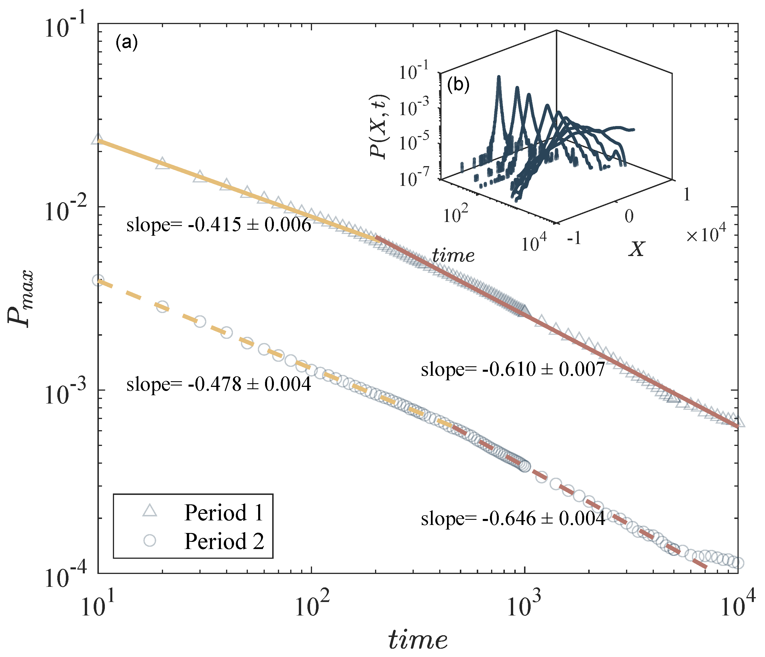
In Figure 2a, we present the peak of the PDF P m a x for Periods 1 and 2, respectively, in relation to time t. In particular, both time periods exhibit a power law relationship between the peak of the PDF and time, expressed as P m a x t H . Linear curve fitting is applied to the data of Periods 1 and 2, respectively, to measure the power law slope ( H = 1 / α ). We note that a transition in the H values is observed for both datasets, signifying a shift in the diffusion mode. For Period 1, the Hurst exponent H is 0.415 ± 0.006 at small time intervals and 0.610 ± 0.007 at large time intervals, corresponding to the values of α = 2.41 ± 0.03 and α = 1.64 ± 0.02 , respectively. For Period 2, the slope is H = 0.478 ± 0.004 at small time intervals and H = 0.646 ± 0.004 at large time intervals, corresponding to the respective values of α = 2.09 ± 0.01 and α = 1.54 ± 0.01 . The anomalous diffusion exponent α is used to distinguish normal (Brownian, α = 2 , H = 0.5 ) from anomalous diffusion ( α 2 , H 0.5 ). The super and subdiffusion regimes correspond to α > 2 , H < 0.5 and 0 < α < 2 , H > 0.5 , respectively [44]. These results suggest that both periods of the Bitcoin time series undergo a transition from a weak subdiffusion regime to a weak superdiffusion regime over an extended period.
Figure 2b illustrates the time evolution of the PDF from 10 min to 1000 min (approximately 16.5 h) of trading time. The PDF at the minimal time interval t = 1 exhibits a heavy-tailed non-Gaussian distribution, gradually flattening and broadening as time progresses. To further explore the fat-tailed distribution of the PDF, it is essential to determine the tail slope of the PDF at the minimum time interval, P ( X * , t = 1 ) . This slope, denoted as α , is crucial for characterizing the type of distribution. The tail exponent for Lévy distribution is calculated as P ( x , t ) x ( 1 + α ) , where 0 < α < 2 [22,23]. The exponent for the q-Gaussian distribution is P ( x , t ) x α , where α = 2 1 q , and 1 < q < 3 [27]. In Figure 3, we present the calculated tail slopes of the PDF for each period. The slopes of the tails for Period 1 and Period 2 are α = 3.95 ± 0.18 and α = 4.04 ± 0.12 , respectively. By comparing these values with the corresponding exponents of Lévy and q-Gaussian distributions, we find that the slopes fall outside the Lévy regime and instead fit well into the q-Gaussian regime. The values of q calculated based on the tail slopes derived using the aforementioned relation are q = 1.51 ± 0.02 and q = 1.50 ± 0.02 for Periods 1 and 2, respectively.
Upon examining the fat-tailed distribution, we found that the PDF in the minimum time interval ( t = 1 ) can be characterized by a q-Gaussian distribution. To substantiate this observation, we conducted a calibration to the q-Gaussian distribution for the PDFs corresponding to both Period 1 and Period 2. The results of this calibration process are shown in Figure 4. This calibration procedure was conducted on a semi-logarithmic scale by applying the relationship described in Equation (7). This method involved taking the natural logarithm of the PDF and fitting it to the simple price return using a linear scale. Figure 4a plots the right branch of the PDF using a logarithmic scale, and Figure 4b illustrates both branches of the PDF in a semi-logarithmic scale. In these figures, the gray dotted curves represent the PDF of the simple price return, while the black curves represent the fitted q-Gaussian distribution. In particular, the fitted distribution captures both the central and tail portions of the PDFs. The q values derived from the semi-logarithmic fitting were determined as q = 1.53 for Period 1 and q = 1.57 for Period 2. Importantly, these values align with the q values fitted from the power law tail slope, affirming the consistency of the results and showing that the diffusion is q-Gaussian.

4.2. Volatility Clustering

We used the autocorrelation function of the absolute returns (|ACF|) to quantify volatility clustering in time series. Note that the autocorrelation function of the raw returns (ACF) is calculated on the incremental price return X * ( t ) using two methods: sample autocorrelation and ensemble autocorrelation. The same calculations apply for |ACF|. The detailed definitions for each method are presented in the following.
The time lag of the autocorrelation is denoted as s, representing real-time intervals in minutes for this study. For each s, the sample autocorrelation is defined as
C ( s ) = t = 1 n s ( X t + s * X * ¯ ) ( X t * X * ¯ ) t = 1 n ( X t * X * ¯ ) 2 ,
where X * is the simple price return, X t + s * is the price return shifted by s minutes, and X * ¯ is the mean value of the price return, calculated as
X * ¯ = 1 n t = 1 n X t * .
We also computed the autocorrelation of the price return for both periods, following the concept of calculating the ensemble autocorrelation. In the context of stochastic processes, the ensemble represents the statistical population of the process, where each member of the ensemble is a possible realization of the process [51,52]. For finance data, where only a singular historical time series exists, constructing this ensemble involves decomposing the time series into an ensemble of subintervals of the data. Here, each trading day effectively constitutes one realization of the dataset, given the recurring nature of market statistics on a daily basis [53]. To build the ensemble in our study, we partitioned the data into discrete segments, where each segment serves as an independent realization of the time series. The total length of the time series for the price return is denoted as N, while the length of each segment is represented as S, so the number of segments is N s = N / S . The ensemble autocorrelation is formulated as
C s = i = 1 N s C s i N s ,
where C s i corresponds to the ith segment within the ensemble. In the typical practice of establishing the ensemble, each segment is often delineated based on individual trading days. However, due to the continuous nature of the Bitcoin market, we chose to employ calendar weeks as partitioning markers for our dataset. Our data are recorded at 10 min intervals, resulting in 6 data points recorded per hour and 1008 data points accumulated each week. We rounded this value to 1000 data points for the length of each segment. Subsequently, we computed the autocorrelation for each segment and averaged it over the ensemble. The error associated with the ensemble autocorrelation was calculated as the standard error within the ensemble.
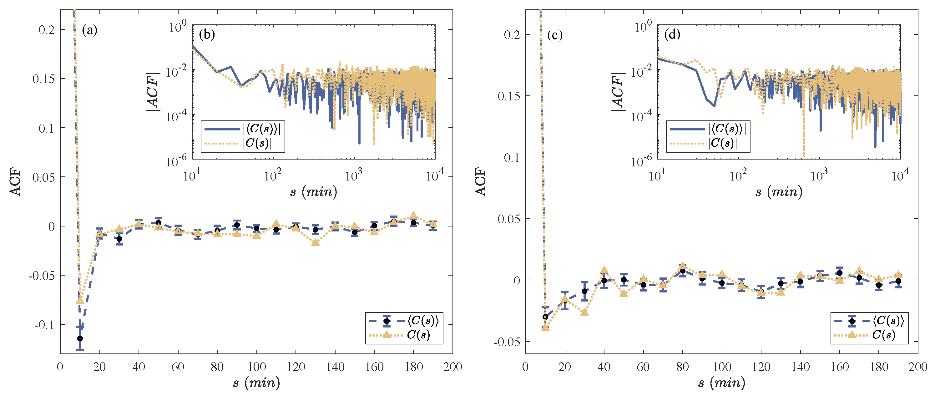
The results of the ACF calculated with both methods are presented in Figure 5 for Periods 1 and 2, respectively. The sample autocorrelation is plotted in yellow, while the ensemble autocorrelation is in blue.
The autocorrelation function of the absolute price returns (|ACF|) is calculated as:
C | X * | ( s ) = t = 1 n s ( | X t + s * | | X * | ¯ ) ( | X t * | | X * | ¯ ) t = 1 n ( | X t * | | X * | ¯ ) 2 ,
The absolute sample autocorrelation functions are illustrated in Figure 5b,d using a log–log scale, corresponding to Periods 1 and 2, respectively. In both time periods, a noticeable power law relationship emerges, particularly evident at short time intervals (below 100 min). Over the longer term, the absolute autocorrelation exhibits a modest yet non-negligible value, persisting notably beyond the 200 min mark ( C ( s ) = 0.002 for larger s). To quantitatively assess this power law behavior, we performed linear fitting, obtaining slope values of 1.17 for Period 1 and 1.07 for Period 2. For a fractional Brownian motion, this slope of absolute autocorrelation is related to the Hurst exponent (H), a relationship established as C ( s ) s 2 2 H [54]. By calculating the Hurst exponent from the power law slope of the absolute autocorrelation, we obtain the respective values of the Hurst exponent for Periods 1 and 2 as H = 0.415 and H = 0.486 . Notably, these values align with the findings detailed in Section 4.1. To further examine the behavior of the short-time autocorrelation, we plotted the ACF for the first 200 min in Figure 5a,c. Both sample and ensemble autocorrelation show negative values at short time lags, indicating an anti-correlated relationship in short time frames. Additionally, ACFs manifest oscillations around 0 from 30 min to 200 min (approximately 2.5 h). Although both the sample autocorrelation and the ensemble autocorrelation exhibit similar characteristics in general, they differ in terms of magnitude. Although there are disparities between the two, these differences are not substantial enough to definitively conclude whether they indicate non-ergodic behavior in the time series or are simply a result of statistical noise.

4.3. Self-Similarity of Detrended PDF of Price Return

While the previous section focused on stylized facts within trended time series, it is important to note that the underlying trend inherent in financial data can potentially influence these characteristics. To address this, we now redirect our attention to exploring the stylized facts in the detrended time series. In previous sections, we found that the Bitcoin market index in Periods 1 and 2 exhibits similar values for the stylized fact quantifiers, despite the differences in the volatility ranges of the two regimes shown in Figure 1. Therefore, in what follows, we focus the analysis on Period 2 only.
Self-similarity in the evolution of the PDF of price return is another important stylized fact in the stock market. We first tested the self-similarity of the trended time series, yet it does not present clear self-similar behavior. Thus, the detrending process is required following the relation described in Equation (21).

4.3.1. Detrending Time Series

The detrending process was carried out using the moving average (MA) method. In MA, a time window is shifted from the start to the end of the time series, and the arithmetic average is used for each time window to record the trend. The two parameters that are vital for MA are the size of the time window t w and the step in which each time window is shifted forward. In this analysis, we used a continuous sliding window with overlaps, and thus the step is 1. These time windows extend from a segment of [ t , t + t w ] to the consecutive window of [ t + 1 , t + t w + 1 ] . To achieve an effective detrending result, it is necessary to select an optimal time window t w for detrending. In this study, the criteria for choosing the optimal time window are set so that the PDFs of the detrended price return P ( x * , t ) show the best convergence to a Gaussian distribution at large time intervals t and the goodness of fit ( R 2 ) indicates a valid fitting ( R 2 0.95 ) for all PDFs.
We tested the time window for detrending from 1 h to 26 weeks to find the best time window that meets the criteria. The optimal time window t w of 1 week is chosen for the detrending, and for each time window, the arithmetic average of the index I ( t ) from [ t , t + t w ] is used as the trend at time t. Considering at the beginning and the end of the time series where t < t w 2 and t > N t w 2 (N is the total length of the time series), the size of the time window is truncated, we define the sliding window with three pieces:
  • For t < t w 2
    I ^ ( t ) = 2 t w + 2 t k = t + 1 ( t w 1 ) / 2 I ( t + k ) ,
  • For t w 2 < t < N t w 2
    I ^ ( t ) = 1 t w k = ( t w 1 ) / 2 ( t w 1 ) / 2 I ( t + k ) ,
  • For t > N t w 2
    I ^ ( t ) = 2 2 N 2 t + t w k = ( t w 1 ) / 2 N t I ( t + k ) ,
with the time step of t = 1 , 2 , 3 N for the index fluctuations.
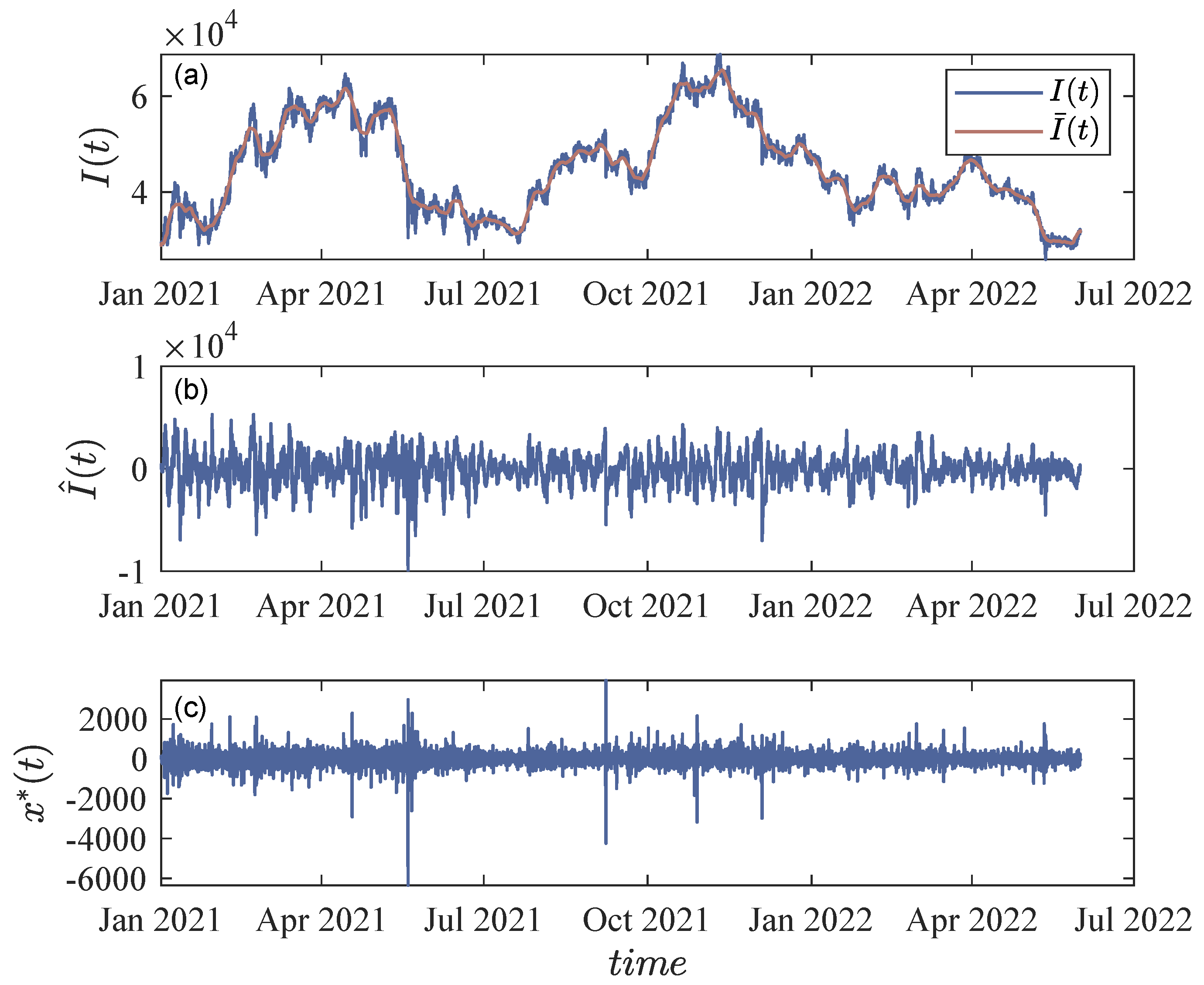
The results of the detrending are shown in Figure 6. Figure 6a presents the trended market index I ( t ) as the blue curve and the trend I ¯ ( t ) in red after applying MA analysis using the optimal time window of 1 week. Figure 6b shows the detrended price as a result of subtracting the trend, following Equation (20). Figure 6c shows the detrended price return by taking the difference of the adjacent terms in the detrended price, using Equation (22).
x * ( t ) = I ^ ( t + 1 ) I ^ ( t ) .

4.3.2. Self-Similarity in PDF of Detrended Price Return

We then test the self-similarity in the detrended price return. Recall the expression of the PDF to be:
P ( x , t ) = 1 ( D t ) H g q x ( D t ) H
where ( D t ) H is the scaling factor, and H = 1 / α is the Hurst exponent, and is related to the parameter characterizing the anomalous diffusion. Taking the result of H = 0.478 in Section 4.1 for time series Period 2, we performed the q-Gaussian fitting to the detrended PDFs at each time t of price return on a semi-log scale, with two fitting parameters q and β = ( D t ) 1 / α to find the scaling factor. The PDFs are rescaled using these factors, and the resulting PDFs were collapsed onto each other, as shown in the gray curves in Figure 7. The collapsed PDF shows good agreement with the q-Gaussian distribution with q = 1.51 , shown as the blue curve.

4.4. Scaling Analysis on the Fractality of Price Return

In the preceding sections, we demonstrated the presence of self-similarity in Bitcoin price returns, suggesting the fractal nature of the time series. In this section, our aim is to determine whether the time series is monofractal or multifractal by performing a scaling analysis. In the latter scenario, self-similarity is preserved, but the Hurst exponent is not unique. Instead, it exhibits a range of values that form a Hurst exponent profile.
Various methods can demonstrate the fractality of a time series, with commonly used approaches including rescaled range analysis (R/S) and detrended fluctuation analysis (DFA). Currently, DFA is becoming a more favored method because of its effectiveness in handling nonstationary time series. In our study, we applied DFA to Bitcoin Period 2 to determine fractality and calculate the Hurst exponent. DFA was performed on trended time series. The first step of DFA involves removing the trend of the original time series by assuming that the trend is the linear fit of each non-overlapping segment.
  • Step 1: For the trended price return with length N, the process of the DFA starts with defining the ‘profile’ of the time series by calculating the mean-centered cumulative sum of the simple price return (X):
    I * ( t ) = k = 1 i X k X ¯ , i = 1 , , N .
    where X ¯ is the mean value of the time series.
The second part of DFA aims to calculate the scaling function F w ( s ) as a function of the time segment s, and w is the order of the mathematical moment. This is achieved by applying the following steps:
  • Step 2: Divide the profile I * ( t ) into non-overlapping segments with the same length s. The number of segments N s is calculated as N s = N / s .
  • Step 3: Calculate the local trend for each segment by a linear least-square fitting of the time series. Then the variance of each segment v from 1 , 2 , 3 N s is calculated using the following equation:
    F 2 ( v , s ) = 1 s i = 1 s ( I * [ ( v 1 ) s + i ] I * ¯ ( v , s ) ) 2 ,
    where I * ¯ ( v , s ) is the mean of each segment of I * ( t ) .
  • Step 4: The statistical moments are calculated utilizing different values of order w:
    F w ( s ) = 1 N s i = 1 N s [ F 2 ( v , s ) ] w / 2 1 / w
This moment analysis identifies the spectrum of the time series. For (monofractal or multifractal) scale-free time series, the following power law is expected:
F w ( s ) s h ( w ) ,
where the Hurst exponent is H = h ( 2 ) . For monofractal time series, the slope of h ( w ) in terms of w is constant (independent of w), and the fractal dimension of the time series satisfies D f = 2 H . Furthermore, the exponent of the autocorrelation function γ satisfies γ = 2 2 H [28]. A multifractal time series is characterized by the spectrum of local slopes that depend on w. The above functions are related to the general wth moment defined as follows
G w ( s ) v = 1 N / s | I * [ v s ] I * [ ( v 1 ) s ] | w
which defines the generalized scaling exponent τ ( w ) via the scaling relation
G w ( s ) s τ ( w ) .
τ ( w ) is shown to be related to h ( w ) via the relation
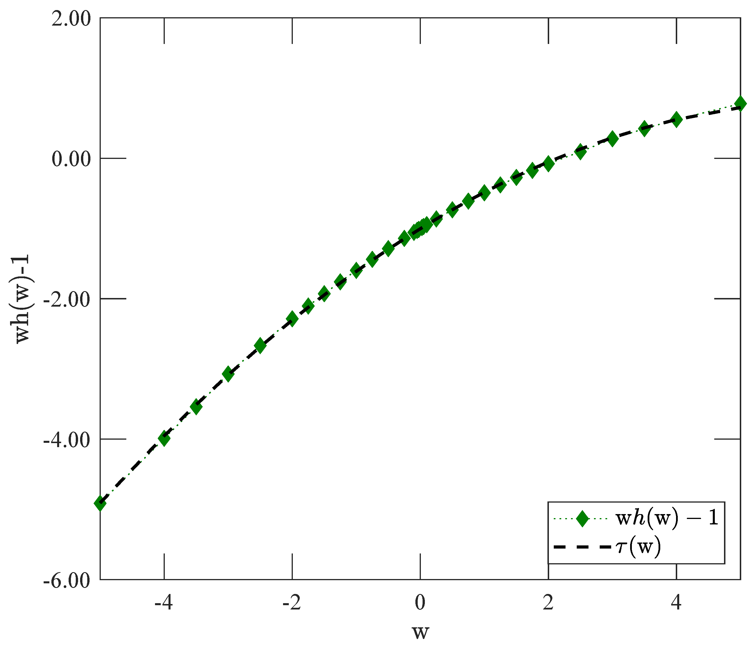
τ ( w ) = w h ( w ) 1 .
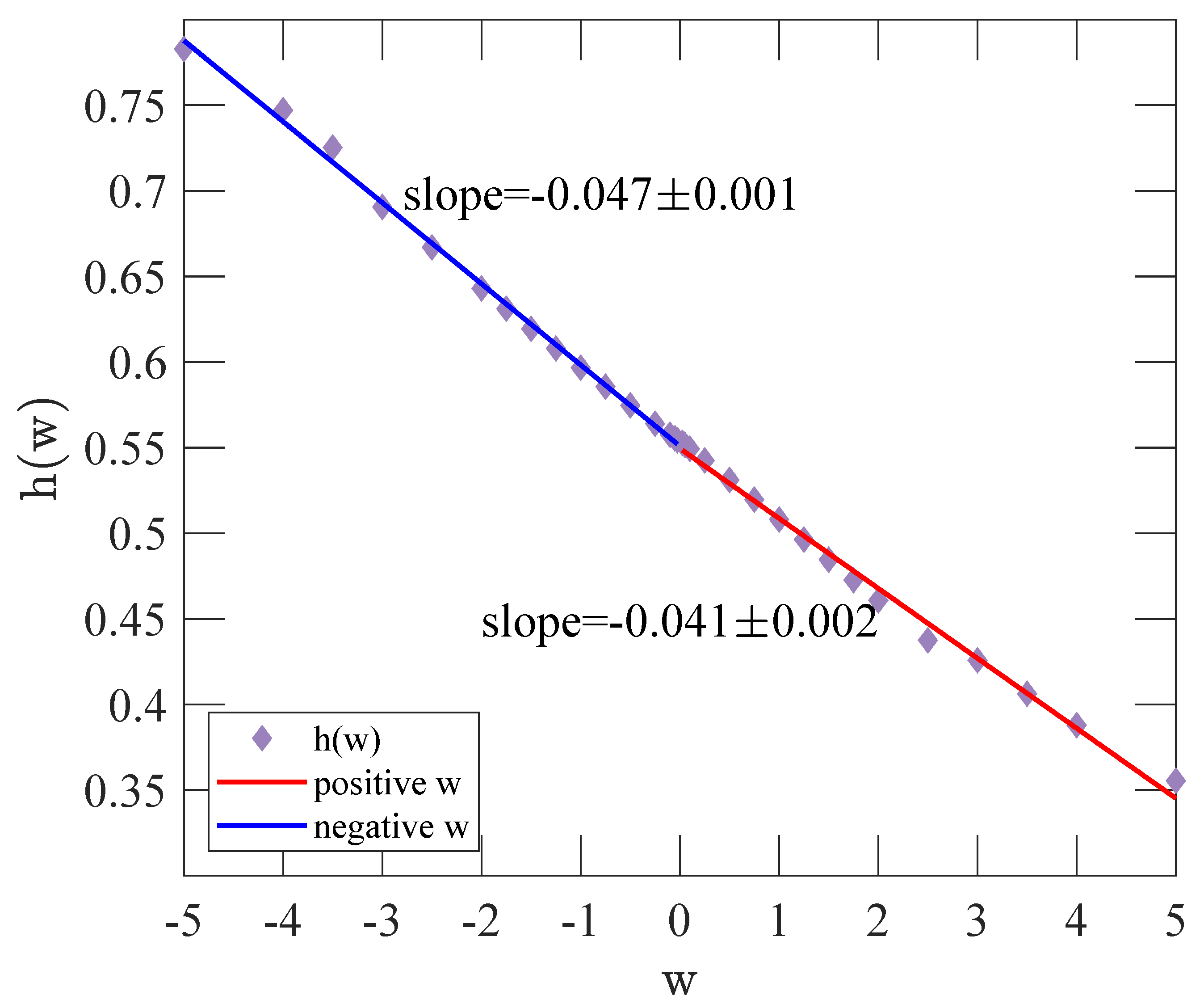
The DFA results are shown in Figure 8 for the positive and negative range of w, showing a power law behavior. The exponents of the scaling behaviors are extracted by using power law fitting (dashed black lines), which is carried out for each order of w. The insets show h ( w ) in terms of w. It is clear that the slope of h ( w ) varies for different w, indicating that the time series is multifractal. Figure 9 shows more clearly the resultant generalized Hurst exponent h ( w ) . Figure 10 presents the relationship between τ ( w ) in terms of h ( w ) , provided that the detrended price return is self-similar and multifractal, since the slope depends on the scale w.
To obtain the spectrum of the Hurst exponent, we have to use a Legendre transformation after performing the detrended fluctuation analysis. In the standard theory of multifractal analysis, one performs the Legendre transformation of the generalized scaling exponent τ ( w ) as a function of h ( w ) , which is based on the linear relation Equation (35). The Legendre transformation of τ ( w ) is then given by
f ( γ ) = γ w τ ( w )
where γ is defined as
γ = τ ( w ) w = h ( w ) w h w .
By substituting Equation (35) in Equation (36), the Legendre transformation of τ ( w ) is found to be
f ( γ ) = w ( γ h ( w ) ) + 1 .
For the case h ( w ) is linear with respect to w, γ is found to be constant, making the Legendre transformation ill-defined. This indicates that γ is not a one-to-one function of w; therefore, it is not invertible to calculate f ( γ ) . To avoid this problem, we add a nonlinear auxiliary term to the function of h ( w ) . More precisely, one adds a nonlinear term to h ( w ) , performs the calculations, and sends the amplitude of the linear term to zero at the end. A similar scenario applies here since the deviations from linearity for h ( w ) are small, i.e., the Legendre transformation results in a constant γ with some fluctuations around. To proceed, we add the following nonlinear term:
h β ( w ) = β w 3 + h ( w ) ,
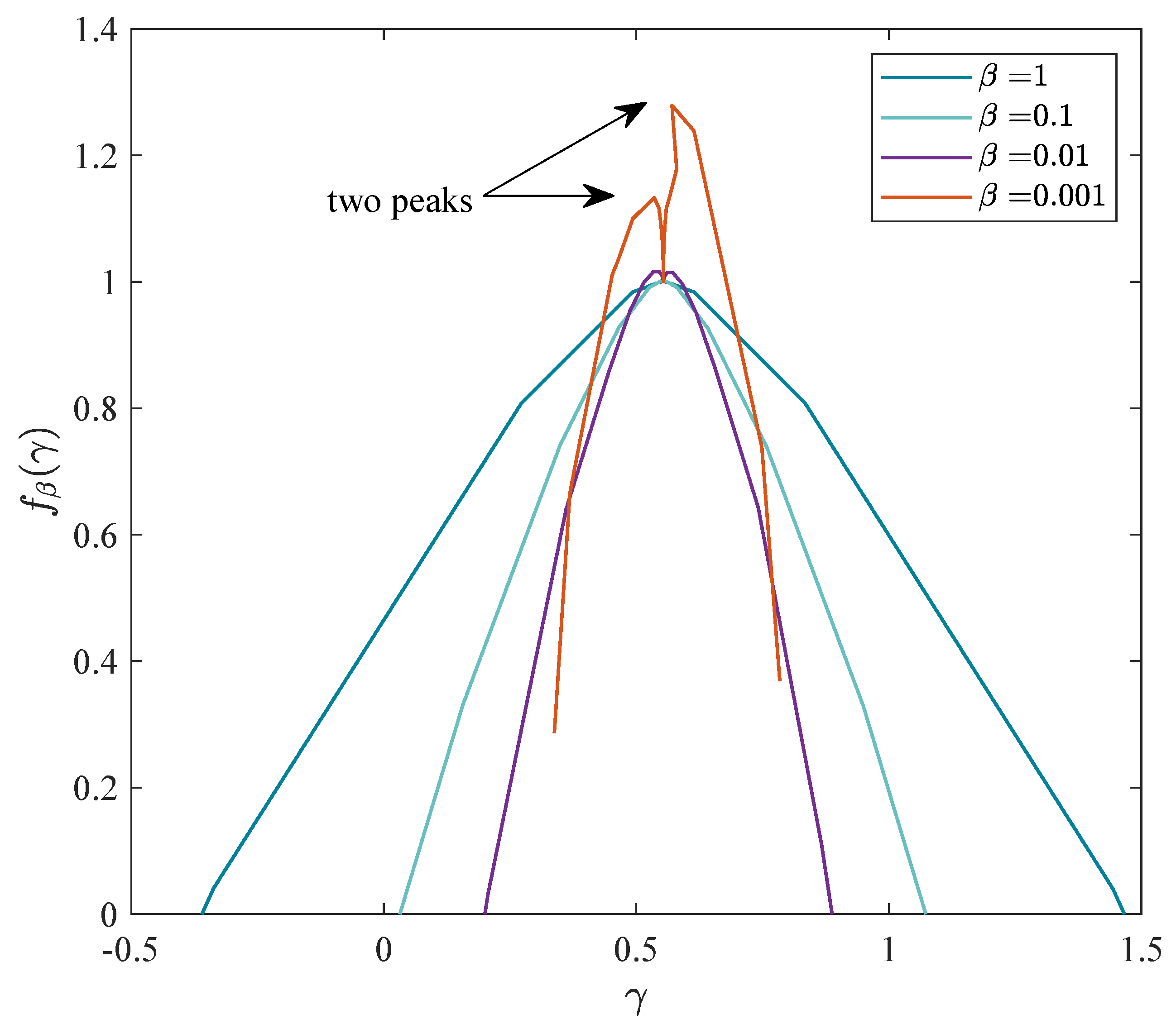
where β is an amplitude. We considered w 3 to make the Legendre transformation one-to-one, that is, f β ( γ ) (obtained using Equation (38) with h ( w ) replaced by h β ( w ) ) is a one-to-one function of γ . This makes Equation (37) invertible, so that γ is easily obtained as a function of w to be used in the other equations. In the end, we should take the limit β 0 , i.e.,
f ( γ ) = lim β 0 f β ( γ ) .
As a simple example to see how this scenario works, consider the simple linear case h ( w ) = a w + b , so that h β ( w ) = β w 3 + a x + b , which gives
γ = 2 β w 3 + b .
or w = ( b γ 2 β ) 1 / 3 , and f β ( γ ) is calculated as:
f β ( γ ) = w ( γ h β ( w ) ) + 1 = b γ 2 β 1 / 2 γ β b γ 2 β a b γ 2 β b + 1
This relation allows us to track and monitor how f ( γ ) approaches f β ( γ ) as β goes to zero. Figure 11 shows the result of f β ( γ ) with different values of β . The results show that as β approaches the limit of 0, two peaks appear, which are shown in the figure. The two peaks represent the two-fractal behavior of the time series. As we already observed in Figure 9, the slopes for positive and negative values of w are slightly different, so one may expect two different classes of exponents, which is consistent with the result that we found based on the nonlinear analysis of Figure 11. Therefore, we conclude that the time series studied here is multifractal.

5. Discussion

We investigated the stylized facts of the Bitcoin time series from 2019 to 2022. The Bitcoin price index was divided into two periods based on volatility changes. Table 1 summarizes the stylized facts observed for Bitcoin and compares them with the well-studied S&P500 (January 1996–May 2018). The S&P500 results are divided into two regimes identified in [27]. Regime 1 corresponds to the superdiffusion regime at very short times and small fluctuations (marked as regime A in [27]), which we traced to small fluctuations about 30 min before the market close. Regime 2 dominates during the official S&P500 trading hours (9:30 a.m.–4:00 p.m. Eastern time) and can be considered stationary after detrending [55]. This daily schedule is important, as market opening and closing times produce characteristic intraday patterns, including the short-lived superdiffusion observed before market close.
The presence of heavy-tailed distributions is a well-known property of financial markets such as the S&P500. Consistently, we found fat-tailed distributions for both Bitcoin periods. This result agrees with those of previous studies on cryptocurrencies [56]. Our analysis further shows that Bitcoin returns are best described by a q-Gaussian distribution, directly comparable to the S&P500. Specifically, we estimate q = 1.51 ± 0.02 for Period 1 and q = 1.50 ± 0.02 for Period 2.
The anomalous diffusion in Bitcoin differs from the S&P500. Although both markets exhibit changes in diffusion behavior, the S&P500 displays a strong superdiffusion regime ( α = 1.26 ± 0.04 , H = 0.79 ) in Regime 1 and a weaker regime ( α = 1.79 ± 0.01 , H = 0.56 ) in Regime 2 [27]. In contrast, Bitcoin changes from sub-diffusion to weak super-diffusion. For Period 1, short intervals yield α = 2.41 ± 0.02 ( H = 0.415 ) and longer intervals α = 1.64 ± 0.02 ( H = 0.610 ). For Period 2, short intervals give α = 2.09 ± 0.01 ( H = 0.478 ) and longer intervals α = 1.54 ± 0.01 ( H = 0.646 ). This indicates antipersistence at short horizons and persistence at longer scales. The q-Gaussian diffusion process also describes Bitcoin, but with lower q values ( q 1.55 ) compared to the S&P500 ( q = 1.71 , q = 2.73 ). This suggests that extreme returns are more frequent in the S&P500.
The autocorrelation function of the raw returns (ACF) and absolute returns (|ACF|) was computed from the Bitcoin returns. The |ACF| shows power law decay, with Hurst exponents moving from below 0.5 in Period 1 ( H = 0.415 ) to closer to 0.5 in Period 2 ( H = 0.465 , Table 1). Both periods show a short-term negative autocorrelation in the ACF, consistent with the feedback trading behavior [57]. For the S&P500, the ACF shows an exponential decay at short times (Regime 1) and a power law at longer times (Regime 2) [55].
At long aggregation horizons, we expect q 1 and H 1 2 . Intuitively, returns over large windows are sums of many 10 min increments; since these increments have finite variance, the classical central limit theorem (CLT) would drive the aggregated distribution toward Gaussian. However, Bitcoin increments are strictly not independent—they exhibit long-range dependence ( power law decay in the autocorrelation of absolute returns)—so the standard CLT assumptions may be violated. In dependent settings, generalized limit theorems govern the asymptotics and can imply slower convergence to normality, modified scaling, or even non-Gaussian attractors. Consequently, the time evolution of q ( t ) and H ( t ) is better analyzed within a generalized CLT framework that accommodates long memory, for example, through variable-order time-dependent diffusion coefficients [58].
From the scaling analysis, both Bitcoin periods are multifractal, consistent with previous work on Bitcoin [4,14] and with evidence from traditional markets [10,37,38,39,40]. Multifractality in Bitcoin probably arises from the clustering of volatility across scales and fat-tailed distributions [36]. The discrepancies of the values of Hurst exponents in the ACF can be attributed to the fact that the time series are not fractal like the fractional Brownian noise, but are instead multifractal. Finally, the fractional derivative parameter ξ calculated from q and H differs between regimes: ξ = 0.62 in Period 1 and ξ = 0.72 in Period 2 for Bitcoin, compared to ξ = 0.72 for the S&P500. These values highlight structural differences in memory and scaling between the crypto and traditional markets.

6. Conclusions

In this work, we analyzed high-frequency Bitcoin returns between 2019 and 2022, focusing on stylized facts such as fat tails, anomalous diffusion, volatility clustering, multifractality, and scaling relations. Our results show that Bitcoin price dynamics exhibit persistent deviations from Gaussian behavior, with q-Gaussian distributions, transitions from subdiffusion to weak superdiffusion, and multifractal scaling properties. These findings align with and extend empirical evidence from traditional equity markets.
Several stylized facts become apparent only after detrending. In particular, we observe approximate self-similarity in the return distribution when detrended with a centered moving average, with an empirically optimal window of about one week. Multifractality is assessed using standard MF-DFA, which removes local trends across scales to recover the scale-dependent Hurst exponent. Looking forward, a unified detrending framework—treating MF-DFA and moving-average filters as interchangeable smoothers—and principled criteria for selecting window lengths and filter parameters (e.g., Wiener–Khintchine consistency and variance–stationarity) should improve robustness and reproducibility. A promising extension is to refine detrending by combining two moving averages: one for the underlying trend and another for local volatility. By adjusting these windows so that residual fluctuations remain spectrally and variance-stable, and by identifying persistent joint shifts in trend and volatility, it may become possible to detect historical regime changes more objectively. Such an approach would provide a reproducible way to separate long-run movements from short-term noise, and deserves further exploration in the context of fractal and fractional modeling.
Beyond documenting stylized facts, our analysis connects directly with the mathematical formulations of fractional porous medium equations. We demonstrated that the nonlinear Fokker–Planck (porous media) equation provides a natural framework to unify fat-tailed distributions, anomalous diffusion, and scaling laws. The introduction of a fractional time parameter ξ through time-stretching or local fractional derivatives bridges empirical fractal properties with fractional porous media dynamics. The hyperscaling relation ξ = H ( 3 q ) shows how fractal geometry, nonlinearity, and fractional calculus jointly govern the observed dynamics.
Thus, Bitcoin time series provide a concrete application where concepts from fractals and fractional porous media equations are not only theoretically consistent but also empirically necessary. This cross-disciplinary connection illustrates how tools originally developed for complex transport in porous media can be applied fruitfully to financial data, highlighting the unifying power of fractal and fractional methodologies. Future research should explore these links further, particularly in relation to generalized central limit theorems and the plausible non-ergodic dynamics of fractional, nonlinear stochastic differential equations.

Author Contributions

Conceptualization, F.A.-M.; Formal analysis, Y.T. and K.A.-C.; Investigation, Y.T.; Data curation, K.A.-C.; Writing—original draft, Y.T.; Writing—review & editing, K.A.-C., M.N.N. and F.A.-M.; Supervision, K.A.-C., M.N.N., M.S.H. and F.A.-M.; Project administration, F.A.-M. All authors have read and agreed to the published version of the manuscript.

Funding

This research received no external funding.

Data Availability Statement

Restrictions apply to the availability of raw data. Data were obtained from LSEG Data & Analytics and are available at https://www.lseg.com/en with the permission of LSEG Data & Analytics.

Conflicts of Interest

The authors declare no conflicts of interest.

References

  1. Mandelbrot, B.B. Self-affine fractals and fractal dimension. Phys. Scr. 1985, 32, 257. [Google Scholar] [CrossRef]
  2. Hilfer, R. Applications of Fractional Calculus in Physics; World Scientific: Singapore, 2000. [Google Scholar]
  3. Gharari, F.; Arias-Calluari, K.; Alonso-Marroquin, F.; Najafi, M.N. Space-time fractional porous media equation: Application on modeling of S&P500 price return. Phys. Rev. E 2021, 104, 054140. [Google Scholar]
  4. Takaishi, T. Statistical properties and multifractality of Bitcoin. Phys. A Stat. Mech. Its Appl. 2018, 506, 507–519. [Google Scholar] [CrossRef]
  5. Tang, Y.; Gharari, F.; Arias-Calluari, K.; Alonso-Marroquin, F.; Najafi, M. Variable-order porous media equations: Application on modeling the S&P500 and Bitcoin price return. Phys. Rev. E 2024, 109, 024310. [Google Scholar]
  6. Corbet, S.; Lucey, B.; Urquhart, A.; Yarovaya, L. Cryptocurrencies as a financial asset: A systematic analysis. Int. Rev. Financ. Anal. 2019, 62, 182–199. [Google Scholar] [CrossRef]
  7. Nakamoto, S. Bitcoin: A Peer-to-Peer Electronic Cash System. 2008. Available online: https://nakamotoinstitute.org/library/bitcoin/ (accessed on 3 August 2023).
  8. Global Cryptocurrency Charts. 2023. Available online: https://coinmarketcap.com/charts/ (accessed on 3 August 2023).
  9. Stoyanov, S.V.; Rachev, S.T.; Racheva-Yotova, B.; Fabozzi, F.J. Fat-Tailed Models for Risk Estimation. J. Portf. Manag. 2011, 37, 107–117. [Google Scholar] [CrossRef]
  10. Chen, F.; Tian, K.; Ding, X.; Miao, Y.; Lu, C. Finite-size effect and the components of multifractality in transport economics volatility based on multifractal detrending moving average method. Phys. A Stat. Mech. Its Appl. 2016, 462, 1058–1066. [Google Scholar] [CrossRef]
  11. Scalas, E.; Gorenflo, R.; Luckock, H.; Mainardi, F.; Mantelli, M.; Raberto, M. Anomalous waiting times in high-frequency financial data. Quant. Financ. 2004, 4, 695–702. [Google Scholar] [CrossRef]
  12. Takaishi, T. Time-varying multifractality in Bitcoin volatility. PLoS ONE 2021, 16, e0261217. [Google Scholar] [CrossRef]
  13. Kakinaka, S.; Umeno, K. Cryptocurrency market efficiency in short- and long-term horizons during COVID-19: An asymmetric multifractal analysis approach. Financ. Res. Lett. 2022, 46, 102319. [Google Scholar] [CrossRef]
  14. Shrestha, K. Multifractal detrended fluctuation analysis of return on Bitcoin. Int. Rev. Financ. 2021, 21, 312–323. [Google Scholar] [CrossRef]
  15. Masoudi, M.; Ito, T. Complexity Analysis of Financial Time Series Using Multifractal and Entropy Measures. arXiv 2025, arXiv:2501.12345. [Google Scholar] [CrossRef]
  16. Kaldor, N.; Hague, D.C. Capital Accumulation and Economic Growth. In The Theory of Capital; International Economic Association Series; Palgrave Macmillan UK: London, UK, 1961; pp. 177–222. [Google Scholar]
  17. Arias-Calluari, K.; Alonso-Marroquin, F.; Najafi, M.N.; Harré, M. Methods for forecasting the effect of exogenous risks on stock markets. Phys. A Stat. Mech. Its Appl. 2021, 568, 125587. [Google Scholar] [CrossRef]
  18. Malmsten, H.; Teräsvirta, T. Stylized facts of financial time series and three popular models of volatility. Eur. J. Pure Appl. Math. 2010, 3, 443–477. [Google Scholar]
  19. Segnon, M.; Bekiros, S. Forecasting volatility in bitcoin market. Ann. Financ. 2020, 16, 435–462. [Google Scholar] [CrossRef]
  20. Bariviera, A.F.; Basgall, M.J.; Hasperué, W.; Naiouf, M. Some stylized facts of the Bitcoin market. Phys. A Stat. Mech. Its Appl. 2017, 484, 82–90. [Google Scholar] [CrossRef]
  21. Mandelbrot, B. The Variation of Certain Speculative Prices. J. Bus. 1963, 36, 394. [Google Scholar] [CrossRef]
  22. Lèvy, P. Thèorie de lÀddition des Variables Alèatoires; Gauthier–Villars: Paris, France, 1937. [Google Scholar]
  23. Mantegna, R.N.; Stanley, H.E. Stochastic Process with Ultraslow Convergence to a Gaussian: The Truncated Lévy Flight. Phys. Rev. Lett. 1994, 73, 2946–2949. [Google Scholar] [CrossRef]
  24. Mantegna, R.N.; Stanley, H.E. Introduction to Econophysics: Correlations and Complexity in Finance; Cambridge University Press: Cambridge, UK, 1999. [Google Scholar]
  25. Borland, L. Microscopic dynamics of the nonlinear Fokker–Planck equation: A phenomenological model. Phys. Rev. E 1998, 57, 6634–6642. [Google Scholar] [CrossRef]
  26. Malamud, B. Tails of natural hazards. Phys. World 2003, 17, 31–35. [Google Scholar] [CrossRef]
  27. Alonso-Marroquin, F.; Arias-Calluari, K.; Harré, M.; Najafi, M.N.; Herrmann, H.J. Q-Gaussian diffusion in stock markets. Phys. Rev. E 2019, 99, 062313. [Google Scholar] [CrossRef] [PubMed]
  28. Beran, J. Statistics for Long-Memory Processes, 1st ed.; Taylor and Francis: London, UK, 2017. [Google Scholar]
  29. Lo, A.W. Long-Term Memory in Stock Market Prices. Econometrica 1991, 59, 1279–1313. [Google Scholar] [CrossRef]
  30. Ding, Z.; Granger, C.W.J.; Engle, R.F. A long memory property of stock market returns and a new model. J. Empir. Financ. 1993, 1, 83–106. [Google Scholar] [CrossRef]
  31. De Sousa Filho, F.N.M.; Silva, J.N.; Bertella, M.A.; Brigatti, E. The Leverage Effect and Other Stylized Facts Displayed by Bitcoin Returns. Braz. J. Phys. 2021, 51, 576–586. [Google Scholar] [CrossRef]
  32. Kumar, R. 2—Risk and return. In Valuation; Kumar, R., Ed.; Academic Press: San Diego, CA, USA, 2016; pp. 47–72. [Google Scholar] [CrossRef]
  33. De Silva, H.; McMurran, G.M.; Miller, M.N. 14 - Diversification and the Volatility Risk Premium. In Factor Investing; Jurczenko, E., Ed.; Elsevier: Amsterdam, The Netherlands, 2017; pp. 365–387. [Google Scholar] [CrossRef]
  34. Ghosh, B.; Bouri, E.; Wee, J.B.; Zulfiqar, N. Return and volatility properties: Stylized facts from the universe of cryptocurrencies and NFTs. Res. Int. Bus. Financ. 2023, 65, 101945. [Google Scholar] [CrossRef]
  35. Mandelbrot, B.B. The Fractal Geometry of Nature; W. H. Freeman and Company: New York, NY, USA, 1982; p. 495. [Google Scholar]
  36. Lahmiri, S.; Bekiros, S. Chaos, randomness and multi-fractality in Bitcoin market. Chaos Solitons Fractals 2018, 106, 28–34. [Google Scholar] [CrossRef]
  37. Gu, R.; Chen, H.; Wang, Y. Multifractal analysis on international crude oil markets based on the multifractal detrended fluctuation analysis. Phys. A Stat. Mech. Its Appl. 2010, 389, 2805–2815. [Google Scholar] [CrossRef]
  38. Lee, M.; Song, J.W.; Park, J.H.; Chang, W. Asymmetric multi-fractality in the U.S. stock indices using index-based model of A-MFDFA. Chaos Solitons Fractals 2017, 97, 28–38. [Google Scholar] [CrossRef]
  39. Mali, P.; Mukhopadhyay, A. Multifractal characterization of gold market: A multifractal detrended fluctuation analysis. Phys. A Stat. Mech. Its Appl. 2014, 413, 361–372. [Google Scholar] [CrossRef]
  40. Wang, F.; Liao, G.; Li, J.; Li, X.; Zhou, T. Multifractal detrended fluctuation analysis for clustering structures of electricity price periods. Phys. A Stat. Mech. Its Appl. 2013, 392, 5723–5734. [Google Scholar] [CrossRef]
  41. Önalan, O. Self-similarity and multifractality in financial asset returns. In Proceedings of the 1st International Conference on Computational Finance and its Applications, Bologna, Italy, 21–23 April 2004; pp. 289–295. [Google Scholar]
  42. Bachelier, L. Théorie de la spéculation. Ann. Sci. De L’École Norm. Supérieure 1900, 17, 21–86. [Google Scholar] [CrossRef]
  43. Black, F.; Scholes, M. The Pricing of Options and Corporate Liabilities. J. Political Econ. 1973, 81, 637–654. [Google Scholar] [CrossRef]
  44. Sposini, V.; Krapf, D.; Marinari, E.; Sunyer, R.; Ritort, F.; Taheri, F.; Selhuber-Unkel, C.; Benelli, R.; Weiss, M.; Metzler, R.; et al. Towards a robust criterion of anomalous diffusion. Commun. Phys. 2022, 5, 305. [Google Scholar] [CrossRef]
  45. Tsallis, C. Possible generalization of Boltzmann-Gibbs statistics. J. Stat. Phys. 1988, 52, 479–487. [Google Scholar] [CrossRef]
  46. Tsallis, C.; Anteneodo, C.; Borland, L.; Osorio, R. Nonextensive statistical mechanics and economics. Phys. A Stat. Mech. Its Appl. 2003, 324, 89–100. [Google Scholar] [CrossRef]
  47. Queirós, S.M.D. On non-Gaussianity and dependence in financial time series: A nonextensive approach. Quant. Financ. 2005, 5, 475–487. [Google Scholar] [CrossRef]
  48. Panyagometh, K. The effect of COVID-19 and US monetary policy on Bitcoin and stock market volatility: An application of DCC-GARCH model. Humanit. Soc. Sci. Commun. 2024, 11, 1735. [Google Scholar] [CrossRef]
  49. Nguyen, K.Q. The correlation between the stock market and Bitcoin during COVID-19 and other uncertainty periods. Financ. Res. Lett. 2022, 46, 102284. [Google Scholar] [CrossRef] [PubMed]
  50. Wȩglarczyk, S. Kernel density estimation and its application. ITM Web Conf. 2018, 23, 00037. [Google Scholar] [CrossRef]
  51. McCauley, J.L. Time vs. ensemble averages for nonstationary time series. Phys. A Stat. Mech. Its Appl. 2008, 387, 5518–5522. [Google Scholar] [CrossRef]
  52. Lahiri, A. Chapter 7—Optical Coherence: Statistical Optics. In Basic Optics; Elsevier Inc.: Amsterdam, The Netherlands, 2016; pp. 605–696. [Google Scholar]
  53. Bassler, K.E.; McCauley, J.L.; Gunaratne, G.H. Nonstationary increments, scaling distributions, and variable diffusion processes in financial markets. Proc. Natl. Acad. Sci. USA 2007, 104, 17287–17290. [Google Scholar] [CrossRef] [PubMed]
  54. Kantelhardt, J.W.; Zschiegner, S.A.; Koscielny-Bunde, E.; Havlin, S.; Bunde, A.; Stanley, H.E. Multifractal detrended fluctuation analysis of nonstationary time series. Phys. A Stat. Mech. Its Appl. 2002, 316, 87–114. [Google Scholar] [CrossRef]
  55. Arias-Calluari, K.; Najafi, M.N.; Harré, M.S.; Tang, Y.; Alonso-Marroquin, F. Testing stationarity of the detrended price return in stock markets. Phys. A Stat. Mech. Its Appl. 2022, 587, 126487. [Google Scholar] [CrossRef]
  56. Zhang, W.; Wang, P.; Li, X.; Shen, D. Some stylized facts of the cryptocurrency market. Appl. Econ. 2018, 50, 5950–5965. [Google Scholar] [CrossRef]
  57. Karaa, R.; Slim, S.; Goodell, J.W.; Goyal, A.; Kallinterakis, V. Do investors feedback trade in the Bitcoin—and why? Eur. J. Financ. 2021, 30, 1951–1971. [Google Scholar] [CrossRef]
  58. Jiang, Y.; Nie, H.; Ruan, W. Time-varying long-term memory in Bitcoin market. Financ. Res. Lett. 2018, 25, 280–284. [Google Scholar] [CrossRef]
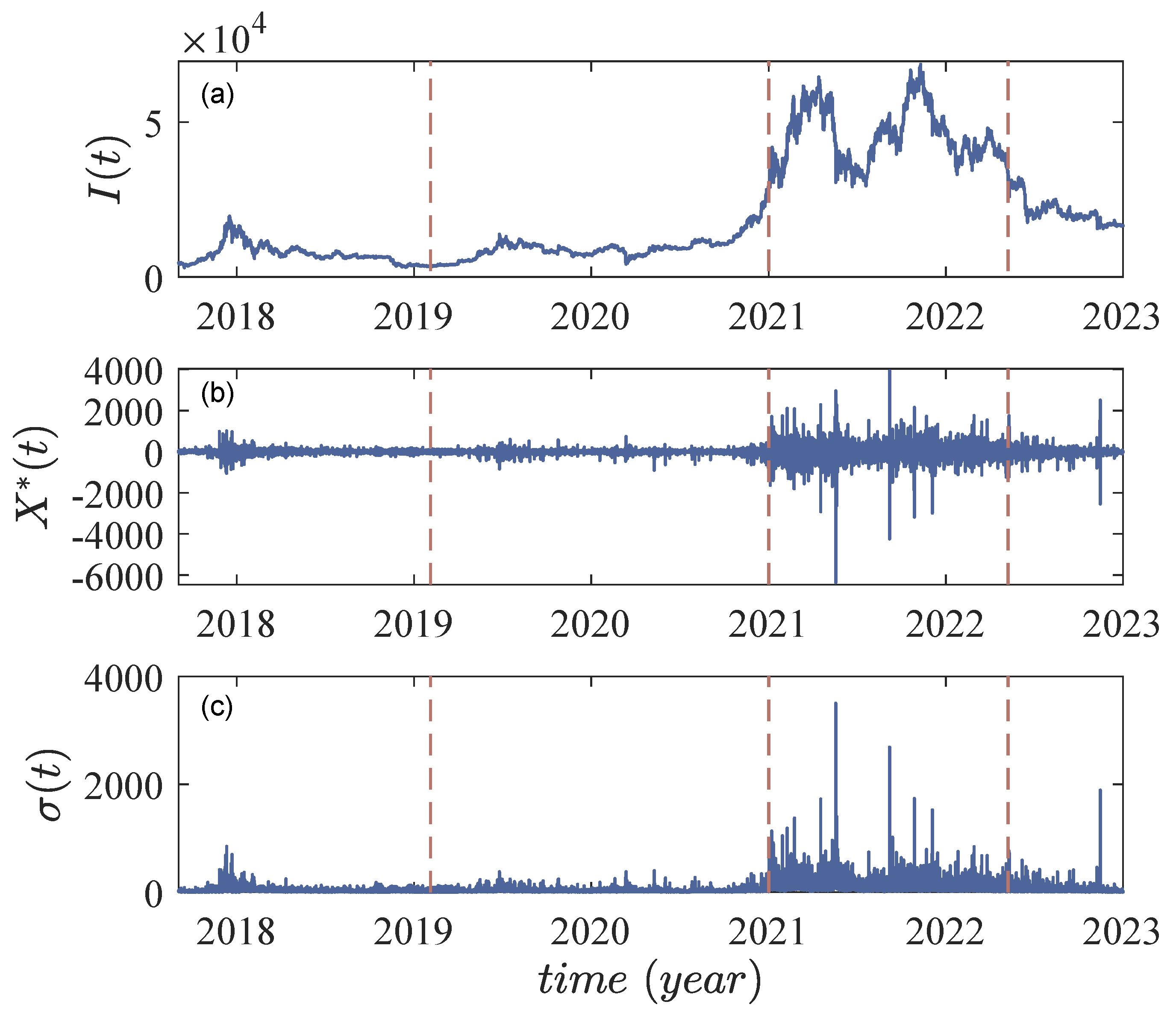
Figure 1. (a) Bitcoin market index I ( t ) from 03/09/2017 to 31/12/2022. (b) Simple price return X * ( t ) obtained from I ^ ( t ) following Equation (22). (c) The standard deviation σ ( t ) of simple price return calculated by using a 1 h moving window, where σ ( t ) = 1 N 1 t = 1 N ( X * ( t ) μ ) 2 , X i * indicates a specific segment of the price return, and μ is the mean value of that segment.
Fractalfract 09 00635 g001
Figure 2. (a) Time evolution of the peak of the PDF for Periods 1 and 2 in the log–log scale shown in black markers; the time is given in minutes. Two well-defined slopes can be observed for each period. The colored lines show the fitted slope of the power law relation. Both periods experience a transition from a weak subdiffusion regimen to a weak superdiffusion regime over time. (b) Time evolution of the PDF for Period 2 from 10 min to 1000 min. The PDFs present distinctive peaks and heavy tails at small time intervals and become flat as the time interval increases.
Fractalfract 09 00635 g002
Figure 3. Tail slope of PDF at the minimum time interval t 0 for Period 1 and 2, respectively, in log–log scale. The dotted gray lines are the PDFs of price return, and the colored lines show the fitted slope of the tail for each time period. The fitted slopes show that the tail slope of the tail for each time period. The fitted slopes show that the tail slope is outside the Lévy regime, and fits to a q-Gaussian distribution.
Fractalfract 09 00635 g003
Figure 4. q-Gaussian fitting conducted in semi-log scale for PDFs of simple price return at t 0 for both Period 1 and 2. The gray dotted curves are the PDFs and the black curves are the fitted q-Gaussian distribution. (a) The right branches of the PDFs for Periods 1 and 2 are plotted in log–log scale, respectively. (b) The full PDF and the fitted distribution are plotted on a semi-log scale.
Fractalfract 09 00635 g004
Figure 5. Sample and ensemble autocorrelation with fitting for Periods 1 and 2. For both periods, anti-correlation is observed for short times, and weak long-term autocorrelation is presented. (a) For Period 1, ensemble ACF is plotted in blue, and sample ACF is plotted in yellow. Anti-correlation is observed in short times with periodicity. The decay of anti-correlation of the raw return are fitted to the law C ( s ) s 2 H * 2 cos ( b s ) . (b) Absolute sample and ensemble ACF of Period 1 plotted in log–log scale, representing a power law relation. A linear fitting in the log–log scale measures the slope of the power law relation as −1.17. (c) For Period 2, ensemble ACF is plotted in blue, and sample ACF is plotted in yellow. Anti-correlation is also observed in short times with periodicity fitted by C ( s ) s 2 H * 2 cos ( b s ) . (d) Absolute sample and ensemble ACF of Period 2 plotted in log–log scale, with a power law relation at initial times. A linear fitting in the log–log scale measures the slope of the power law relation as −1.07.
Fractalfract 09 00635 g005
Figure 6. Results from detrending analysis for Period 2. (a) Trended price index I ( t ) is shown as the blue curve, and the trend I ¯ ( t ) obtained from the MA is shown as the red curve. (b) The detrended price index I ^ ( t ) was obtained by subtracting the trend from the price index. (c) Detrended price return x * ( t ) calculated from the detrended price index.
Fractalfract 09 00635 g006
Figure 7. The gray curves show the collapse of the PDF of the detrended price return for Bitcoin Period 2. The collapsed PDFs are fitted with a q-Gaussian distribution (blue curve) with q = 1.51 .
Fractalfract 09 00635 g007
Figure 8. Calculation of the statistical function F w on Bitcoin price return for Period 2 using Equation (31). The function of F w vs. s display power laws F w ( s ) s h ( w ) , where h ( w ) depends on w. This feature demonstrates that the time series is multifractal. (a) Calculated F w ( s ) function with a negative range of w; each w value presents a power law relationship. (b) Profile of h ( w ) for negative w values. (c) Calculated F w ( s ) function with a positive range of w; each w value presents a power law relationship. (d) Profile of h ( w ) for positive w values.
Fractalfract 09 00635 g008
Figure 9. Evaluation of the scale exponents h ( w ) of detrended Bitcoin price return for Period 2. This profile of scale exponent can be described using linear relationships for positive and negative w, with the slope being 0.047 ± 0.001 for negative w, and 0.041 ± 0.002 for positive w, respectively.
Fractalfract 09 00635 g009
Figure 10. Generalized scaling exponent τ ( w ) of the detrended price return for Period 2, showing the relation τ ( w ) = w h ( w ) 1 .
Fractalfract 09 00635 g010
Figure 11. Result for f β ( γ ) with varying β values from 1 to 0.001. As β decreases, f β ( γ ) becomes narrower. When β = 0.001 , two peaks are presented as shown in the red curve.
Fractalfract 09 00635 g011
Table 1. Summary of stylized facts. The exponent ξ for the fractional derivative is calculated from the exponent q of the fat-tailed distribution and the Hurst exponent H of the short-time anomalous diffusion using the hyperscaling relation ξ = H ( 3 q ) . The values presented for the S&P500 correspond to the analyzed period from 1996 to 2018 per minute [27,55].
Stylized FactEquationBTC 1BTC 2S&P500 1S&P500 2
Fat-tailed Distribution P ( x , t ) x 2 1 q q = 1.51 q = 1.50 q 1.70 N/A
Anomalous Diffusion
(Short time-intervals)
P ( 0 , t ) t H , H = 1 / α H = 0.42
α = 2.41
H = 0.48
α = 2.09
H = 0.56
α = 1.79
H = 0.79
α = 1.26
q-Gaussian Diffusion P ( x , t ) = 1 ( D t ) H g q ( x ( D t ) H ) q = 1.53 q = 1.57 q = 1.71 q = 2.73
Volatility Clustering C | x | ( s ) s 2 H 2 H = 0.42 H = 0.47 N/AN/A
Multiscaling Analysis F w ( s ) s h ( w ) N/A H = 0.461 H = 0.48 H = 0.48
Fractional derivative ξ = H ( 3 q ) ξ = 0.62 ξ = 0.72 ξ = 0.72 ξ = 0.21
Disclaimer/Publisher’s Note: The statements, opinions and data contained in all publications are solely those of the individual author(s) and contributor(s) and not of MDPI and/or the editor(s). MDPI and/or the editor(s) disclaim responsibility for any injury to people or property resulting from any ideas, methods, instructions or products referred to in the content.