Discrete-Time Design of Fractional Delay-Based Repetitive Controller with Sliding Mode Approach for Uncertain Linear Systems with Multiple Periodic Signals

Abstract

In this paper, a discrete-time design of a fractional internal model-based repetitive controller with a sliding mode approach is presented for uncertain linear systems subject to repetitive trajectory and periodic disturbance. The proposed algorithm, named a fractional delay-based repetitive sliding mode controller (FD-RSMC), aims to enhance tracking accuracy, transient response, and robustness against parametric variations beyond what is offered by conventional repetitive controllers. First, a fractional delay-based repetitive controller (FD-RC) that allows the periodic delay steps to be noninteger is presented to improve the trajectory tracking accuracy and good disturbance compensation of multiple periodic signals. Second, a sliding mode control (SMC) with a discrete-time reaching law is systematically incorporated into FD-RC to improve transient response, especially during the learning period of FD-RC, and also to provide system robustness against model uncertainties. Finally, the stability proof of the closed-loop system with the proposed controller is assessed based on a delayed-sliding mode-reaching condition. Finally, comparative simulation studies are presented to demonstrate the superior performance of the proposed controller.

1. Introduction

Tracking and rejecting periodic signals are common challenges in many control applications. Repetitive control (RC) is an effective learning control strategy for tracking and/or compensating a periodic signal. RC outperforms classical control schemes, such as proportional-integral-derivative (PID), because RC can learn repetitive signal values and then use them as control input [1]. Recently, RC has become increasingly popular and has been applied to a variety of applications, including optical-stabilized systems [2], piezo-actuated nanoscanners [3], mechanical ventilation systems [4], substrate carrier systems [5], and robotic leg prostheses [6]. Additionally, RC has gained popularity in active vibration damping control, where it is effectively used to suppress periodic disturbances, as demonstrated in [7,8,9].

Inou et al. [10] first introduced a continuous-time RC model based on an internal model principle of Wonham and Francis [11]. According to the internal model principle, the periodic signal model must be incorporated into the closed-loop system for error-free tracking of the periodic signal. The continuous-time RC model in [10] was represented by an internal model ${\mathsf{I}}_c\left(s\right)={\mathrm{e}}^{-s{T}_r}/(1-{\mathrm{e}}^{-s{T}_r})$, where $T_r$ is a period of trajectory $r\left(t\right)$. The continuous-time internal model ${\mathsf{I}}_c\left(s\right)$ is marginally stable and exhibits an infinite dimensional structure as the model has infinite poles located at an imaginary axis: $\pm jk\omega$, where $k=1,2,\cdots ,\infty$. Due to marginally stable poles and infinite dimension structure, the continuous-time model ${\mathsf{I}}_c\left(s\right)$ is sensitive to high-frequency disturbances and model uncertainties. Additionally, the internal model can only be used for a properly stable plant with a relative degree of zero. A strict proper plant, on the other hand, is modeled in many engineering situations [12]. In addition, the internal model is limited to a properly stable plant with a relative degree of zero, while many engineering applications are modeled as strictly proper plants. 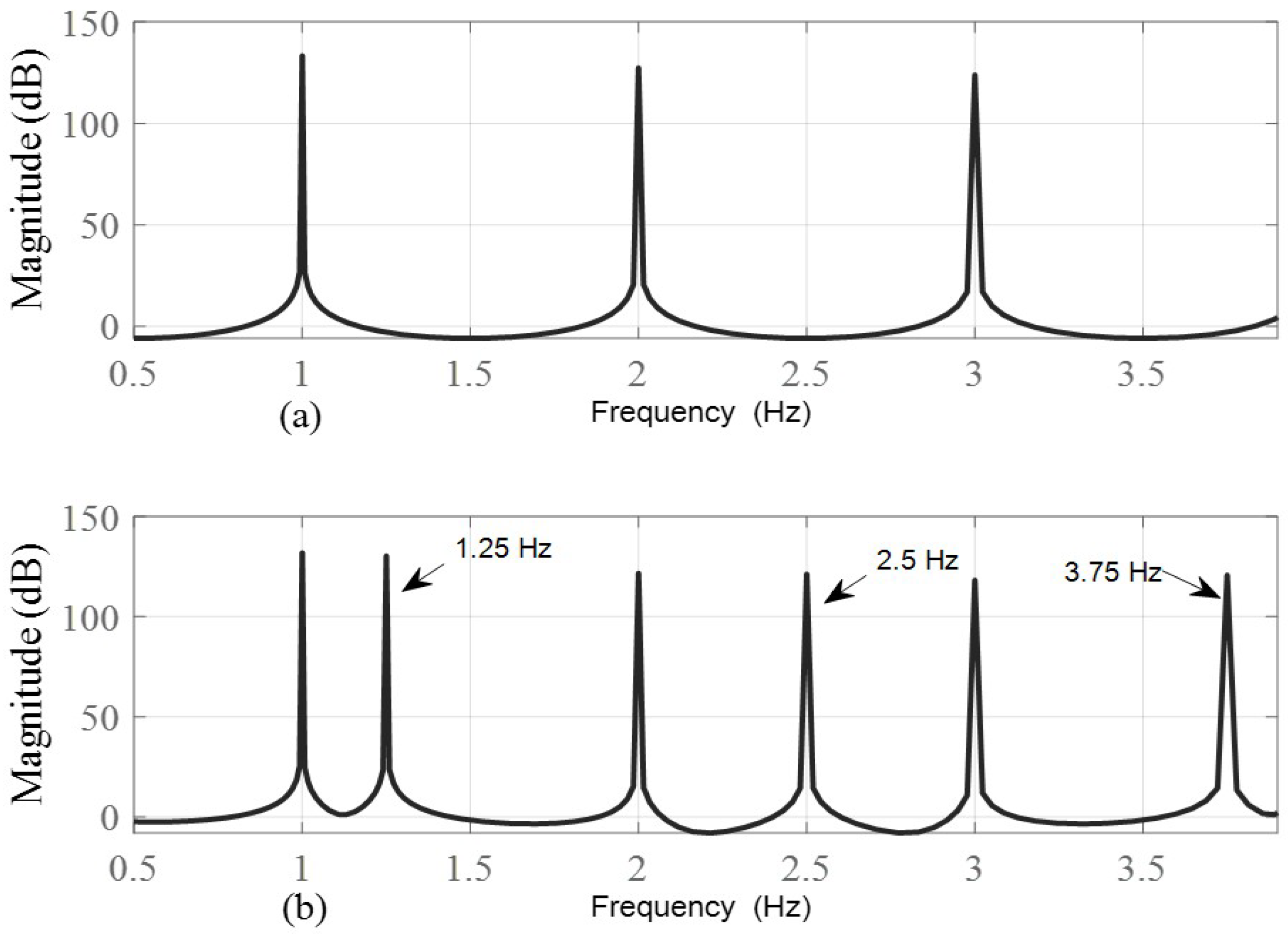In order to avoid an infinite-dimensional structure, a discrete-time internal model-based RC was introduced in [13] and formulated as ${\mathsf{I}}_d\left(z\right)=z^{-N_r}/(1-z^{-N_r})$, where $N_r=T_r/T\in \mathbb{Z}$ is an integer number of samples per trajectory period and T is a sampling period. The discrete-time RC possesses a finite-dimensional structure due to the fact that its poles are finite and evenly spaced and located at a unit circle. For repetitive signals with the frequency $h/T_r$ (where $h=1,2,\cdots ,N_r/2$), this discrete model generates a null tracking error. This means that the tracking is limited to the Nyquist components of the periodic signal, encompassing only the fundamental frequency and its harmonics $h/T_r$.

However, the tracking performance and stability of a discrete-time RC system depend on the two following assumptions: (1) the trajectory period $T_r$ is precisely known, which gives an integer delay length, $N_r$; (2) an accurate model of the plant is also known. The first common assumption in the design of discrete-time RC is that the trajectory period ($T_r$) is known and fixed. In practice, however, the trajectory and sampling periods are subject to variation, which can change the delay length ($N_r$) from an integer to a fractional value. Rounding the delay length to the nearest integer value is the simplest method for implementing fractional delay length. However, the actual reference and the internal model will experience a frequency mismatch due to this solution. As a result, the tracking accuracy of the system is compromised. The second assumption implies that the stability of the RC system relies on the known plant model. This is due to the fact that RC is a model-based learning control scheme requiring an accurate model of the plant, especially one needed to design a compensator. A compensator is part of RC besides an internal model, which is used to compensate plant model dynamics and stabilize the closed-loop RC system. Hence, the tracking and robust performance of a standalone RC system is generally susceptible to the trajectory’s period variation and plant model uncertainties.

Several studies have focused on improving the performance of RCs when subjected to period variation [14,15,16,17,18,19]. The adaptive-based RC approach is demonstrated in the works of [14,15,16] since the proposed scheme operates by adapting the sampling period T in order to preserve the integer value $N_r$. The adaptive-based RC solution gives rise to system complexity and implementation due to the requirement to adjust the sampling period. Moreover, the adjustment in the sampling period will also change the dynamics of the discrete-time plant model. Other than adaptive-based RC, higher-order-based RC found in [17,18,19] was also presented to enhance the tracking performance of the systems under period variation. Instead of using one-period delay, $z^{-N_r}$, such as with general RC, higher-order-based RC employs weighting multiple delays ($w_1{z}^{-N_r},w_2{z}^{-2N_r},\cdots ,w_m{z}^{-p{N}_r}$) in constructing the internal model. Here, $w_1,w_2,...w_m$ are the weights, and m is the highest order of RC. The higher-order-based RC aims to extend the high gains of the internal model to the neighboring region around the nominal targeted frequency ($1/T_r$). Thus, higher-order-based RC can improve the trajectory-tracking performance at the neighboring frequencies, e.g., $(1/T_r)\pm {\Delta }_f$, where ${\Delta }_f$ represents a minor frequency shift. However, due to multiple delays $z^{-N_r},z^{-2N_r},\cdots ,z^{-m{N}_r}$, the higher-order-based solution requires large memories and converges slower compared to the general RC.

In contrast to adaptive-based RC, which seeks to maintain the integer value $N_r$, and higher-order-based RC, which extends the internal model’s high gains to the neighboring region of the targeted frequency, we implement fractional internal model-based RC in this study. The fractional internal model-based RC is later referred to as fractional delay-RC (FD-RC), emphasizing that in situations involving period variation, the delay length, $N_r$, constructing the internal model does not need to be an integer. Here, the fractional time delay is also rooted in fractional calculus, which has been extensively studied and widely used in controller design and dynamics modeling in various applications, as evidenced in [20,21,22,23,24,25]. In [20], the Riemann-Liouville definition of fractional derivatives for the purpose of recreating the spatial structure of the fractional Schrödinger equation for electrical screening potentials was investigated. An explicit solution formula for fractional delay difference systems and a discrete delayed Mittag-Leffler matrix function were derived in [21]. Practical applications of fractional calculus for synthesizing a fractional-order PID controller to control bifurcation in fractional-order small-world networks were demonstrated in [22]. Additionally, the work [23] designed a reduced-order discrete-time fractional-order PID controller. Furthermore, the authors of [24] developed model-based fractional order controllers for time-delay processes in servo systems, while the authors of [25] dealt with the design of complex fractional order speed controllers for induction motors. These studies demonstrate the wide range of applications and potential benefits of fractional calculus in enhancing controller performance and dynamics modeling. In contrast to [20,21,22,23,24,25], we concern ourselves with the fractional delay design in discrete time, which is required to construct an accurate internal model of the RC system.

In order to address the second limitation of general RC, an integrated sliding mode controller (SMC) is utilized to ensure robustness in the presence of model uncertainties. SMC is a widely recognized control scheme that operates on the principle of switching control and attempts to steer a sliding function in the direction of a designated sliding surface. A discrete-time SMC has been widely exploited in much of the literature [26,27,28,29,30,31,32], and here, the discrete-time SMC with a linear switching function will be incorporated into the FD-RC. Numerous research studies have been conducted on the utilization of sliding mode control with a supplementary control scheme, such as repetitive control, as reported in [33,34,35,36,37,38]. In [33], a repetitive sliding mode controller incorporating an exponential-based bi-power reaching law for three-phase voltage source inverters was introduced. An integral sliding mode control scheme based on repetitive control was developed in [34] for uncertain repetitive processes with the presence of matched uncertainties, external disturbances, and norm-bounded nonlinearities. A repetitive sliding mode controller with a modified RC was designed in [35] for uncertain linear systems. An adaptive smooth second-order sliding mode repetitive control method for a class of nonlinear systems with unknown disturbances and uncertainties was proposed [36]. In [37], a discrete-time low-order sliding mode repetitive controller was presented for a class of uncertain linear systems affected by band-limited periodic disturbances and parametric uncertainties. Lu et al. [38] presented an enhanced sliding-mode repetitive learning control scheme using the wavelet transform, which speeds up the learning process.

In contrast to previous studies (references [33,34,35,36,37,38]), the main aim of this study is to address the issue of tracking and/or rejecting disturbances within a particular class of uncertain linear systems that exhibit multiple periodic signals. These systems may exhibit variability in both the reference signal and disturbance signal periods, which results in non-integer discrete-time delay lengths. Therefore, in the context of this study, our aim is to develop a novel control approach known as the fractional delay-based repetitive sliding mode controller (FD-RSMC). The objective of this controller is also to overcome the primary constraints of conventional RC systems by combining fractional delay-based repetitive control (FD-RC) with sliding mode control (SMC), as previously described. Here, FD-RC is applied to keep the delay length fixed to the period of the actual reference or disturbance. Thus, the period disparity between the controller and the actual reference due to period variation can be avoided, as the RC system’s tracking accuracy depends on this condition. The fractional delay term is realizable and straightforward to use because it can be implemented as an independent, stable, and causal IIR filter. The coefficients of the corresponding filter can be obtained by utilizing the Thiran formula [39,40], as illustrated in the works in [41,42]. In contrast to the internal model examined in this study, which deals with the reference or disturbance model, the research described in [41,42] focused on the fractional order design of the RC compensator with the objective of developing a closed-loop RC system stabilizing controller. Next, SMC is systemically incorporated into FD-RC to improve the robustness of the system against parametric uncertainties. Moreover, SMC is also capable of enhancing the transient response of the system, especially during the learning process of the RC part. In this study, a systematic integration between FD-RC and SMC is described, and a stability analysis is performed. Simulation and comparison studies over an integer delay-based repetitive sliding mode controller (ID-RSMC) and standalone RC are provided to show the effectiveness of the proposed design. In order to emphasize the significance of our work, the main contributions are highlighted as follows:

(1)

A novel and systemic integration is established between FD-RC and SMC with the objective of overcoming the constraints of general RC. The proposed approach subsequently addresses the two primary limitations of conventional RC, namely its vulnerability to fluctuations in tracking or disturbance periods and the uncertainties associated with plant models.

(2)

Stability analysis of the FD-RSMC system is carried out based on the reaching condition, and it is proved that the evolution of the sliding function decreases and moves toward the sliding surface. Furthermore, every control parameter utilized in the formulation of the proposed control law is proven to be stable and realizable.

(3)

The implementation of the FD-RC component in the proposed FD-RSMC is feasible due to the substitution of a stable and causal IIR filter for the fractional portion of the RC delay.

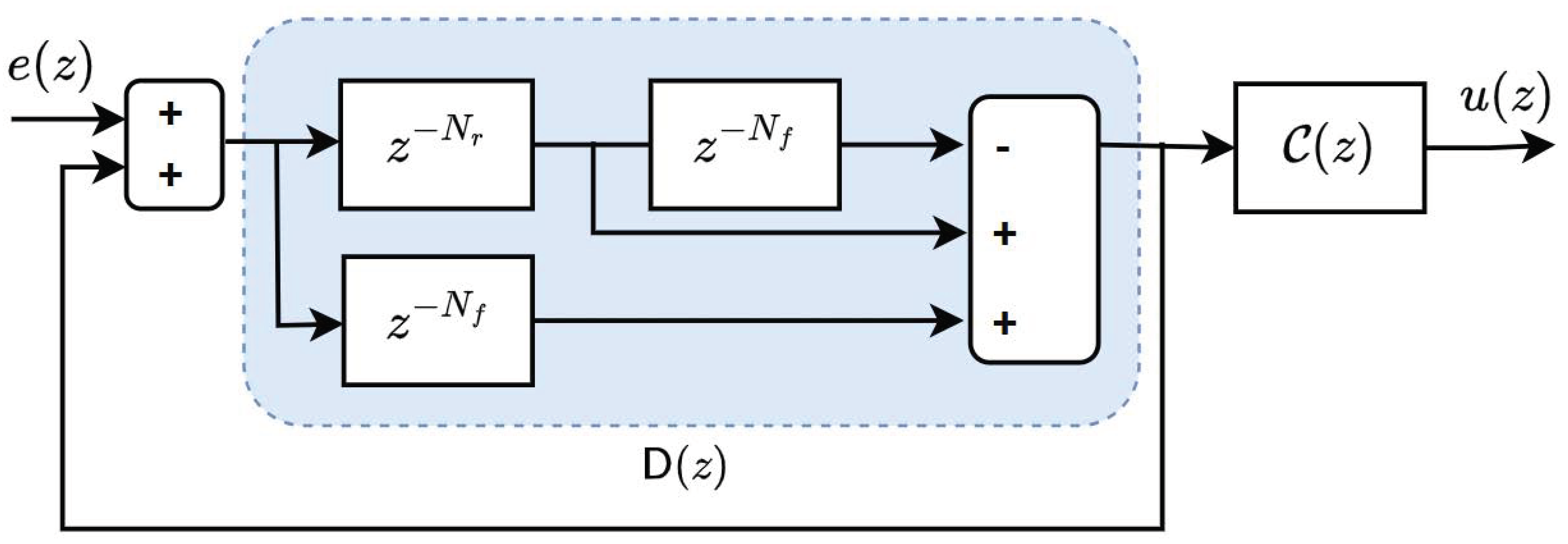
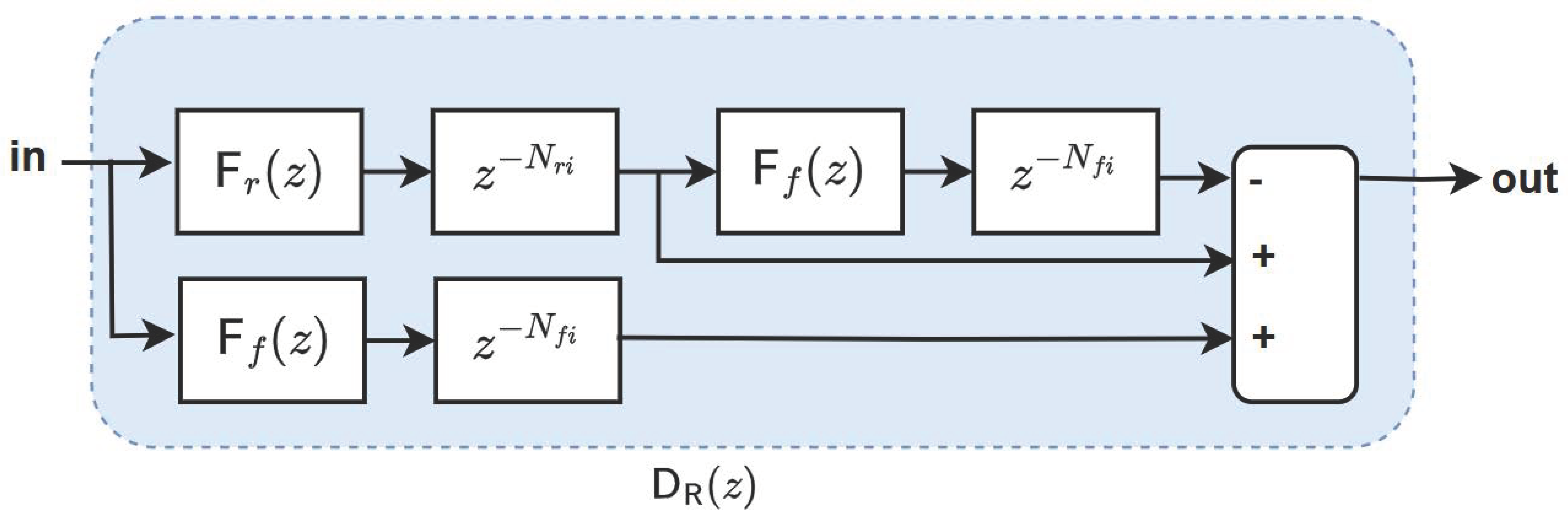
The rest of this paper is structured as follows: Section 2 describes problem formulation and preliminary, which comprises the class of the system, control objective, assumptions used in the design, and the overview of single and two-period general RCs. Section 3 illustrates the main results of the FD-RC and FD-RSMC designs and the stability analysis of the FD-RSMC closed-loop system. Section 4 discusses the simulation and comparison studies, and Section 5 presents the conclusions of the paper.

2. Problem Formulation and Preliminary

2.1. Problem Formulation

We consider a class of uncertain linear systems with internal disturbance in the following form:

$$\begin{array}{c}\hfill \{\mathsf{A}\left(z\right)+{\delta }_{\mathsf{A}}\left(z\right)\}{y}_k=z^{-d}\{\mathsf{B}\left(z\right)+{\delta }_{\mathsf{B}}\left(z\right)\}\left(u_k+f_k\right)\end{array}$$

(1)

where $u_k$, $y_k$, and $f_k$ correspond to control input, system output, and input disturbance at time $t=kT$, respectively, k is a time step, T is the sampling period, $z^{-d}$ is an input delay with d step, $\mathsf{A}\left(z\right)$ and $\mathsf{B}\left(z\right)$ are denumerator and numerator polynomials, respectively, and ${\delta }_{\mathsf{A}}\left(z\right)$ and ${\delta }_{\mathsf{B}}\left(z\right)$ denote the parametric uncertainties of $\mathsf{A}\left(z\right)$ and $\mathsf{B}\left(z\right)$, respectively.

The polynomials $\mathsf{A}\left(z\right)$ and $\mathsf{B}\left(z\right)$ are given as

$$\begin{array}{cc}\hfill \mathsf{A}\left(z\right)& =1+{\mathsf{a}}_1{z}^{-1}+\cdots +{\mathsf{a}}_{\mathsf{m}}{z}^{-\mathsf{m}},\hfill \end{array}$$

(2)

$$\begin{array}{cc}\hfill \mathsf{B}\left(z\right)& ={\mathsf{b}}_0+{\mathsf{b}}_1{z}^{-1}+\cdots +{\mathsf{b}}_{\mathsf{n}}{z}^{-\mathsf{n}},\hfill \end{array}$$

(3)

where $\mathsf{n}<\mathsf{m}$, $\mathsf{m}$, and $\mathsf{n}$ are the degrees of $\mathsf{A}\left(z\right)$ and $\mathsf{B}\left(z\right)$, and $(\mathsf{m}-\mathsf{n})$ is a relative degree of the system (1). Here, $\{{\mathsf{a}}_1,{\mathsf{a}}_2,\cdots ,{\mathsf{a}}_{\mathsf{m}}\}$, and $\{{\mathsf{b}}_0,{\mathsf{b}}_1,\cdots ,{\mathsf{b}}_{\mathsf{n}}\}$ are the nominal parameters of $\mathsf{A}\left(z\right)$ and $\mathsf{B}\left(z\right)$, which are subject to parametric uncertainties ${\delta }_{\mathsf{A}}\left(z\right)$, ${\delta }_{\mathsf{B}}\left(z\right)$, respectively. Note that ${\delta }_{\mathsf{A}}\left(z\right)$ and ${\delta }_{\mathsf{B}}\left(z\right)$ are polynomials that represent parameter changes in $\mathsf{A}\left(z\right)$ and $\mathsf{B}\left(z\right)$, respectively, and can also be viewed as linear functions. The expressions for ${\delta }_{\mathsf{A}}\left(z\right)$ and ${\delta }_{\mathsf{B}}\left(z\right)$ are as follows:

$$\begin{array}{cc}\hfill {\delta }_{\mathsf{A}}\left(z\right)& =\Delta {\mathsf{a}}_1{z}^{-1}+\cdots +\Delta {\mathsf{a}}_{\mathsf{m}}{z}^{-\mathsf{m}},\hfill \end{array}$$

(4)

$$\begin{array}{cc}\hfill {\delta }_{\mathsf{B}}\left(z\right)& =\Delta {\mathsf{b}}_0+\Delta {\mathsf{b}}_1{z}^{-1}+\cdots +\Delta {\mathsf{b}}_{\mathsf{n}}{z}^{-\mathsf{n}}.\hfill \end{array}$$

(5)

Let us consider the tracking error $e_k$, defined as

$$\begin{array}{c}\hfill e_k:=r_k-y_k,\end{array}$$

(6)

where $r_k$ corresponds to the desired trajectory or a reference signal. By rearranging the system (1), we have the representation of system output, $y_k$, and disturbances $v_k$, $p_k$, and ${\mathcal{L}}_k$ as

$$\begin{array}{cc}\hfill y_k& ={\displaystyle \frac{z^{-d}\mathsf{B}\left(z\right)}{\mathsf{A}\left(z\right)}}{u}_k+{\displaystyle \frac{z^{-d}\mathsf{B}\left(z\right)}{\mathsf{A}\left(z\right)}}{f}_k-{\displaystyle \frac{{\delta }_{\mathsf{A}}\left(z\right)}{\mathsf{A}\left(z\right)}}{y}_k+{\displaystyle \frac{z^{-d}{\delta }_{\mathsf{B}}\left(z\right)}{\mathsf{A}\left(z\right)}}{u}_k+{\displaystyle \frac{z^{-d}{\delta }_{\mathsf{B}}\left(z\right)}{\mathsf{A}\left(z\right)}}{f}_k,\hfill \end{array}$$

(7)

$$\begin{array}{cc}\hfill v_k& ={\displaystyle \frac{z^{-d}\mathsf{B}\left(z\right)}{\mathsf{A}\left(z\right)}}{f}_k,\hfill \end{array}$$

(8)

$$\begin{array}{cc}\hfill p_k& =-{\displaystyle \frac{{\delta }_{\mathsf{A}}\left(z\right)}{\mathsf{A}\left(z\right)}}{y}_k+{\displaystyle \frac{z^{-d}{\delta }_{\mathsf{B}}\left(z\right)}{\mathsf{A}\left(z\right)}}{u}_k+{\displaystyle \frac{z^{-d}{\delta }_{\mathsf{B}}\left(z\right)}{\mathsf{A}\left(z\right)}}{f}_k,\hfill \end{array}$$

(9)

$$\begin{array}{cc}\hfill {\mathcal{L}}_k& =v_k+p_k,\hfill \end{array}$$

(10)

where $(v_k,f_k,p_k,{\mathcal{L}}_k)\in \mathbb{R}$, $v_k$ is a filtered periodic disturbance $f_k$, $p_k$ is a parametric disturbance, and ${\mathcal{L}}_k$ is a lump disturbance affecting the system. Then, the system output $y_k$ (7) and tracking error (6) can be rewritten as

$$\begin{array}{cc}\hfill y_k& ={\displaystyle \frac{z^{-d}\mathsf{B}\left(z\right)}{\mathsf{A}\left(z\right)}}{u}_k+{\mathcal{L}}_k.\hfill \end{array}$$

(11)

$$\begin{array}{cc}\hfill e_k& =r_k-{\displaystyle \frac{z^{-d}\mathsf{B}\left(z\right)}{\mathsf{A}\left(z\right)}}{u}_k-{\mathcal{L}}_k.\hfill \end{array}$$

(12)

The objective of this research is to develop a control law $u_k$ for the system (1), which is subject to repetitive trajectory, $r_k$, parametric uncertainties, (${\delta }_{\mathsf{A}},{\delta }_{\mathsf{B}}$), and periodic disturbance, $f_k$, such that the system output $y_k$ precisely follows the trajectory $r_k$ and faster system response and robustness are achieved. In addition, the design also permits a fractional time delay in the control law, which is later proven to be capable of improving the tracking accuracy. The aforementioned goals also imply that the lump disturbance ${\mathcal{L}}_k$ appearing in (12) is maximally compensated, resulting in the tracking error converging to a nearly zero value, $e_k\approx 0$. The following assumptions are made prior to designing the proposed controller to ensure that the research objective is met.

Assumption 1.

The desired trajectory $r_k$ and the disturbance $f_k$ are both periodic with fundamental periods $T_r$ and $T_f$, respectively, where $T_r$ and $T_f$ are known. It is assumed that the trajectory frequency ${\displaystyle \frac{1}{T_r}}$ and the disturbance frequency ${\displaystyle \frac{1}{T_f}}$ are uncorrelated, implying that $({\displaystyle \frac{1}{T_r}})\ne h({\displaystyle \frac{1}{T_f}})$ or $({\displaystyle \frac{1}{T_f}})\ne h({\displaystyle \frac{1}{T_r}})$ for any harmonic number h.

Assumption 2.

The input delay $z^{-d}$, as well as the nominal polynomials $\mathsf{A}\left(z\right)$ and $\mathsf{B}\left(z\right)$, are assumed to be known. Furthermore, $\mathsf{A}\left(z\right)$ and $\mathsf{B}\left(z\right)$ are stable polynomials, meaning that all their roots lie inside the unit circle. The perturbed polynomials $\{\mathsf{A}\left(z\right)+{\delta }_{\mathsf{A}}\left(z\right)\}$ and $\{\mathsf{B}\left(z\right)+{\delta }_{\mathsf{B}}\left(z\right)\}$ remain stable, indicating that the uncertain system (1) is stable and minimum-phase. If the open-loop system is either unstable or nonlinear, a different approach would be necessary for formulating the control law.

2.2. Single and Dual Internal Model-Based RCs

RC is one of the learning control methods that are capable of tracking repetitive trajectory, $r_k$, or/and rejecting the periodic disturbance $f_k$ with zero tracking error. This is due to the inclusion of the internal model representing the model of $r_k$ or/and $f_k$ into the controller. Let a desired trajectory $r_k$ and disturbance $f_k$ be both periodic with basis periods of $T_r$ and $T_f$, respectively. Note that the trajectory frequency ${\displaystyle \frac{1}{T_r}}$ and disturbance frequency ${\displaystyle \frac{1}{T_f}}$ are uncorrelated, implying that ${\displaystyle \frac{1}{T_r}}\ne h{\displaystyle \frac{1}{T_f}}$ or ${\displaystyle \frac{1}{T_f}}\ne h{\displaystyle \frac{1}{T_r}}$ for harmonic number h. The numbers of samples per trajectory and disturbance periods are denoted as $N_r$ and $N_f$ and calculated as $N_r=T_r/T$ and $N_f=T_f/T$, where T is a sampling period. A generic form of RC for a single purpose, e.g., tracking $r_k$ is given by the following control update:

$$\begin{array}{c}\hfill u_k=u_{k-N_r}+\mathcal{C}\left(z\right)e_{k-N_r},\end{array}$$

(13)

which can be transformed into an input-output transfer function as

$$\begin{array}{c}\hfill {\displaystyle \frac{u\left(z\right)}{e\left(z\right)}}=\underset{\mathrm{single}\mathrm{internal}\mathrm{model}}{\underbrace{\left[{\displaystyle \frac{z^{-N_r}}{1-z^{-N_r}}}\right]}}\mathcal{C}\left(z\right).\end{array}$$

(14)

Here, $u_{k-N_r}$ and $e_{k-N_r}$ in (13) are one-cycle delays of input $u_k$ and error $e_k$, respectively, $\mathcal{C}\left(z\right)$ is a compensator generally designed as an inverse plant model, and $z^{-N_r}$ is a delay term with the length of $N_r$. The term $z^{-N_r}/(1-z^{-N_r})$ in (14) is denoted as a single-period internal model, as the model only targets one basis frequency and its harmonics.

For both tracking $r_k$ and rejecting $f_k$, the following two-periods RC law is required:

$$\begin{array}{c}\hfill u_k=\left[\mathsf{D}\left(z\right)\right]u_k+\mathcal{C}\left(z\right)\left[\mathsf{D}\left(z\right)\right]e_k,\end{array}$$

(15)

which is equivalent to the transfer function as follows:

$$\begin{array}{c}\hfill {\displaystyle \frac{u\left(z\right)}{e\left(z\right)}}=\underset{\mathrm{dual}\mathrm{internal}\mathrm{model}}{\underbrace{\left[{\displaystyle \frac{\mathsf{D}\left(z\right)}{1-\mathsf{D}\left(z\right)}}\right]}}\mathcal{C}\left(z\right).\end{array}$$

(16)

In contrast to single-period RC, which employs a one-cycle delay denoted as $z^{-N_r}$, two-period RC is constructed using a delay term denoted as $\mathsf{D}\left(z\right)$. In this context, $\mathsf{D}\left(z\right)$ is represented as multiple time delays and is derived to ensure that the denominator of the internal model matches the following expression:

$$\begin{array}{c}\hfill 1-\mathsf{D}\left(z\right)=\prod _{j=1}^{L}1-z^{-N_j},\end{array}$$

(17)

where L denotes the number of targeted basis frequencies. As our focus is on two fundamental frequencies, specifically the trajectory frequency $1/T_r$ and the disturbance frequency $1/T_f$, $D\left(z\right)$ is consequently modeled as

$$\begin{array}{cc}\hfill 1-\mathsf{D}\left(z\right)& =\prod _{j=1}^{\mathsf{2}}1-z^{-N_j},\hfill \\ \hfill \mathsf{D}\left(z\right)& =1-(1-z^{-N_r})(1-z^{-N_f}),\hfill \\ \hfill \mathsf{D}\left(z\right)& =z^{-N_r}+z^{-N_f}-z^{-N_r-N_f}.\hfill \end{array}$$

(18)

A complete diagram of two-period RC embedding $\mathsf{D}\left(z\right)$ is shown in Figure 1. The other difference between single-period and two-period RCs can be seen from the magnitude-frequency characteristics of their internal models. For instance, given that $T_r=1$ s ($f_r=1$ Hz) and $T_f=0.8$ s ($f_f=1.25$ Hz), the magnitude responses of single- and two-period internal models are plotted in Figure 2. It can be seen from Figure 2 that two-period RC exhibits extra peaks showing the targeted disturbance frequencies $f_f=h\times 1.25$ Hz ($h=1,2,\cdots ,N_f/2$). Therefore, two-period RC here can be applied to simultaneously track the trajectory $r_k$ and reject the disturbance $f_k$.

In order to ensure the asymptotic stability of system (1) with the single internal model-based RC (14), the following conditions must be satisfied [43,44]:

•

The plant model $\mathcal{G}\left(z\right)$ is a stable transfer function. Based on (1), $\mathcal{G}\left(z\right)$ is given by

$$\begin{array}{c}\hfill \mathcal{G}\left(z\right)=z^{-d}{\displaystyle \frac{\mathsf{A}\left(z\right)+{\delta }_{\mathsf{A}}\left(z\right)}{\mathsf{B}\left(z\right)+{\delta }_{\mathsf{B}}\left(z\right)}}.\end{array}$$

(19)

•

The compensator $\mathcal{C}\left(z\right)$ in (14) is such that

$$\begin{array}{c}\hfill {\parallel \left[1-\mathcal{C}\left(z\right)\mathcal{G}\left(z\right)\right]z^{-N_r}\parallel }_{\infty }<1.\end{array}$$

(20)

Similarly, for the dual internal model-based RC (16), the asymptotic stability of system (1) is guaranteed by

•

The plant model $\mathcal{G}\left(z\right)$ is a stable transfer function.

•

The compensator $\mathcal{C}\left(z\right)$ in (16) is such that

$$\begin{array}{c}\hfill {\parallel \left[1-\mathcal{C}\left(z\right)\mathcal{G}\left(z\right)\right]\mathsf{D}\left(z\right)\parallel }_{\infty }<1.\end{array}$$

(21)

Consider the nominal model of (19), which is given by ${\mathcal{G}}_o\left(z\right)=z^{-d}{\displaystyle \frac{\mathsf{A}\left(z\right)}{\mathsf{B}\left(z\right)}}$ and is stable and a minimum-phase system. Assuming this nominal model is known, the compensator $\mathcal{C}\left(z\right)$ can be selected as the inverse of the nominal model. That is

$$\begin{array}{c}\hfill \mathcal{C}\left(z\right)=z^d{\displaystyle \frac{\mathsf{B}\left(z\right)}{\mathsf{A}\left(z\right)}}.\end{array}$$

(22)

However, the presence of uncertainties ${\delta }_{\mathsf{A}}\left(z\right)$ and ${\delta }_{\mathsf{B}}\left(z\right)$ may cause the condition (21) to be violated, potentially leading to system instability. This issue highlights a potential drawback of standalone RC when dealing with model uncertainties.

Next, we define a repetition model $\mathsf{E}\left(z\right)$, which is a denominator of the internal model of the two-period RC. The repetition model $\mathsf{E}\left(z\right)$ is given by

$$\begin{array}{c}\hfill \mathsf{E}\left(z\right)=1-\mathsf{D}\left(z\right),\end{array}$$

(23)

By assuming that $r_k$ and $f_k$ are perfectly periodic with periods $T_r$ and $T_f$, respectively, then the following properties apply:

$$\begin{array}{cc}\hfill \mathsf{E}\left(z\right)r_k& =0\to r_k-\left[\mathsf{D}\left(z\right)\right]r_k=0,\hfill \end{array}$$

(24)

$$\begin{array}{cc}\hfill \mathsf{E}\left(z\right)f_k& =0\to f_k-\left[\mathsf{D}\left(z\right)\right]f_k=0.\hfill \end{array}$$

(25)

The repetition model $\mathsf{E}\left(z\right)$ is an important part of the dual internal model-based RC, which will later be incorporated into SMC to obtain the proposed controller.

3. Controller Design

3.1. Fractional Delay-Based Repetitive Controller (FD-RC)

In the majority of RC designs, the delay lengths $N_r$ and $N_f$ in (18) must be integers, making the delay terms $z^{-N_r}$ and $z^{-N_f}$ realizable. In the case where $N_r$ and $N_f$ are non-integer, then $N_r$ and $N_f$ are rounded to the closest integer values. For instance, consider the trajectory period to be $1.03$ s and the sampling period to be $0.004$ s. Then, we obtain $N_r$ as $257.5$. In order to implement the fractional time-delay $z^{-257.5}$, the straightforward solution is obtained by rounding the delay length to the closest integer value, that is $z^{-257}$. However, the rounded delay does not represent the actual trajectory period (i.e., 0.004 × $257=1.028$ s $\ne 1.03$ s), which later will introduce certain steady-state errors. In this work, the delay lengths $N_r$ and $N_f$ are not required to be integers, so they can both be fractional. Suppose that both delay lengths $N_r$ and $N_f$ are fractional numbers that can be decomposed into

$$\begin{array}{cc}\hfill N_r& =N_{ri}+{\mathsf{n}}_r,\hfill \end{array}$$

(26)

$$\begin{array}{cc}\hfill N_f& =N_{fi}+{\mathsf{n}}_f,\hfill \end{array}$$

(27)

where $N_{ri}<N_r$ and $N_{fi}<N_f$, $\{N_{ri},N_{fi}\}$ are both integers, and $\{{\mathsf{n}}_r,{\mathsf{n}}_f\}$ are both fractional numbers. Consequently, the delay terms $z^{-N_r}$ and $z^{-N_f}$ can be separated into

$$\begin{array}{cc}\hfill z^{-N_r}& =z^{-N_{ri}}\left[z^{-{\mathsf{n}}_r}\right],\hfill \end{array}$$

(28)

$$\begin{array}{cc}\hfill z^{-N_f}& =z^{-N_{fi}}\left[z^{-{\mathsf{n}}_f}\right],\hfill \end{array}$$

(29)

As illustrated in [41,42], the fractional delays $\{z^{-{\mathsf{n}}_r},z^{-{\mathsf{n}}_f}\}$ can be approximated by infinite impulse response (IIR) filters $\{{\mathsf{F}}_r\left(z\right),{\mathsf{F}}_f\left(z\right)\}$, the coefficients of which are calculated based on the Thiran formula as follows [39,40]:

$$\begin{array}{c}\hfill z^{-{\mathsf{n}}_r}\approx {\mathsf{F}}_r\left(z\right)={\displaystyle \frac{{\mathsf{c}}_p{z}^p+{\mathsf{c}}_{p-1}{z}^{p-1}+\cdots +{\mathsf{c}}_{1}z+1}{z^p+{\mathsf{c}}_1{z}^{p-1}+\cdots +{\mathsf{c}}_p}},\end{array}$$

(30)

where $p=\mathrm{ceil}\left({\mathsf{n}}_r\right)$, and $\{{\mathsf{c}}_1,{\mathsf{c}}_2,\cdots ,{\mathsf{c}}_p\}$ are calculated according to

$$\begin{array}{c}\hfill {\mathsf{c}}_i={(-1)}^i\left({\displaystyle \genfrac{}{}{0pt}{}{p}{i}}\right)\prod _{j=0}^p{\displaystyle \frac{{\mathsf{n}}_r-p+j}{{\mathsf{n}}_r-p+j+i}},\forall i:1,2,\cdots ,p,\mathrm{where}\left({\displaystyle \genfrac{}{}{0pt}{}{p}{i}}\right)={\displaystyle \frac{p!}{i!(p-i)!}}.\end{array}$$

(31)

Then, similar procedures are applied to obtain ${\mathsf{F}}_f\left(z\right)$. Finally, $\mathsf{D}\left(z\right)$ in (18) can be rewritten as

$$\begin{array}{c}\hfill {\mathsf{D}}_{\mathsf{R}}\left(z\right)={\mathsf{F}}_r\left(z\right)z^{-N_{ri}}+{\mathsf{F}}_f\left(z\right)z^{-N_{fi}}-{\mathsf{F}}_r\left(z\right){\mathsf{F}}_f\left(z\right)z^{-N_{ri}-N_{fi}},\end{array}$$

(32)

where ${\mathsf{D}}_{\mathsf{R}}\left(z\right)$ represents the fractional delay model of $\mathsf{D}\left(z\right)$ (18), and the realization of ${\mathsf{D}}_{\mathsf{R}}\left(z\right)$ is illustrated in Figure 3.

Note that from a practical perspective, the fractional delay-based RC is feasible and straightforward to implement in real-time applications. The controller is constructed using the fractional delay terms, which are divided into integer and fractional components, both of which are realizable. The fractional part of the delay can be implemented by replacing the delay with a stable and causal IIR filter, with coefficients obtained using the Thiran formula. Meanwhile, the integer portion is also realizable, as it is essentially a transport delay.

3.2. Fractional Delay-Based Repetitive Sliding Mode Controller (FD-RSMC)

In this subsection, we describe how to integrate FD-RC with a nonlinear control scheme such as a sliding mode controller (SMC). Incorporating SMC into the controller design requires the establishment of a sliding surface and reaching law functions. The following linear sliding surface is considered

$$\begin{array}{c}\hfill {\mathsf{s}}_k=\mathsf{H}\left(z\right)e_k,\end{array}$$

(33)

where $\mathsf{H}\left(z\right)$ is a polynomial with zeros inside the unit circle, $e_k$ is the tracking error, and ${\mathsf{s}}_k$ is a sliding surface. Based on the studies in [26,45], the discrete-time delayed reaching law is used as follows:

$$\begin{array}{c}\hfill {\mathsf{s}}_{k+d}-{\mathsf{s}}_k=-k_1{\mathsf{s}}_k-k_2\mathrm{sat}\left({\displaystyle \frac{{\mathsf{s}}_k}{k_3}}\right),\end{array}$$

(34)

where $k_1$, $k_2$, and $k_3$ are positive constants and $0<(1-k_1)<1$. The expression (34) is identical to (35) and (36) as follows:

$$\begin{array}{cc}\hfill {\mathsf{s}}_{k+d}& =(1-k_1){\mathsf{s}}_k-k_2\mathrm{sat}\left({\displaystyle \frac{{\mathsf{s}}_k}{k_3}}\right),\hfill \end{array}$$

(35)

$$\begin{array}{cc}\hfill {\mathsf{s}}_k& =(1-k_1){\mathsf{s}}_{k-d}-k_2\mathrm{sat}\left({\displaystyle \frac{{\mathsf{s}}_{k-d}}{k_3}}\right).\hfill \end{array}$$

(36)

The saturation function $\mathrm{sat}\left({\displaystyle \frac{{\mathsf{s}}_{k-d}}{k_3}}\right)$ used in (36) is selected over the original switching function, which employs a sign function to reduce the chattering phenomenon. This saturation function, commonly known as a boundary layer, smooths the sliding mode control signal. Here, $\mathrm{sat}\left({\displaystyle \frac{{\mathsf{s}}_{k-d}}{k_3}}\right)$ is characterized as

$$\begin{array}{c}\hfill \mathrm{sat}\left({\displaystyle \frac{{\mathsf{s}}_{k-d}}{k_3}}\right)=\left\{\begin{array}{cc}1,& {\mathsf{s}}_{k-d}>k_3,\hfill \\ {\displaystyle \frac{1}{k_3}}{\mathsf{s}}_{k-d},& -k_3<{\mathsf{s}}_k<k_3,\hfill \\ -1,& {\mathsf{s}}_{k-d}<-k_3,\hfill \end{array}\right.\end{array}$$

(37)

and is illustrated in Figure 4.

Let us rewrite (12) to have the following error dynamics:

$$\begin{array}{cc}\hfill \mathsf{A}\left(z\right)e_k& =-z^{-d}\mathsf{B}\left(z\right)u_k+\mathsf{A}\left(z\right)r_k-{\mathcal{W}}_k,\hfill \end{array}$$

(38)

where ${\mathcal{W}}_k=\mathsf{A}\left(z\right){\mathcal{L}}_k$. By multiplying the repetitive model (23) by the sliding surface (33), we have

$$\begin{array}{c}\hfill {\mathsf{s}}_k-\left[\mathsf{D}\left(z\right)\right]{\mathsf{s}}_k=\mathsf{H}\left(z\right)e_k-\mathsf{H}\left(z\right)\left[\mathsf{D}\left(z\right)\right]e_k,\end{array}$$

(39)

where $\left[\mathsf{D}\left(z\right)\right]{\mathsf{s}}_k$ is equivalent to

$$\begin{array}{c}\hfill \left[\mathsf{D}\left(z\right)\right]{\mathsf{s}}_k={\mathsf{s}}_{k-N_r}+{\mathsf{s}}_{k-N_f}-{\mathsf{s}}_{k-N_r-N_f}.\end{array}$$

(40)

For simplicity, we will use the notation $\left[\mathsf{D}\left(z\right)\right]{\mathsf{s}}_k$ in the derivation instead of those on the right-hand side of (40). By adopting minimum control variance in [46], the polynomial $\mathsf{H}\left(z\right)$ is made equivalent to

$$\begin{array}{c}\hfill \mathsf{H}\left(z\right)=\mathsf{A}\left(z\right)\mathsf{R}\left(z\right)+z^{-d}\mathsf{S}\left(z\right),\end{array}$$

(41)

where $\mathsf{R}\left(z\right)$ and $\mathsf{S}\left(z\right)$ are solutions to polynomial matching (41). Then, (39) can be expressed as

$$\begin{array}{c}\hfill {\mathsf{s}}_k-\left[\mathsf{D}\left(z\right)\right]{\mathsf{s}}_k=\mathsf{A}\left(z\right)\mathsf{R}\left(z\right)e_k-\mathsf{A}\left(z\right)\mathsf{R}\left(z\right)\left[\mathsf{D}\left(z\right)\right]e_k+\mathsf{S}\left(z\right)e_{k-d}-\mathsf{S}\left(z\right)\left[\mathsf{D}\left(z\right)\right]e_{k-d}\end{array}$$

(42)

Consider the nominal plant with no uncertainties and disturbances, i.e., ${\mathcal{L}}_{\mathsf{A}k}=0$, which yields the error dynamics as follows:

$$\begin{array}{cc}\hfill \mathsf{A}\left(z\right)e_k& =-z^{-d}\mathsf{B}\left(z\right)u_k+\mathsf{A}\left(z\right)r_k.\hfill \end{array}$$

(43)

Substituting (43) to (42) yields:

$$\begin{array}{cc}\hfill {\mathsf{s}}_k-\left[\mathsf{D}\left(z\right)\right]{\mathsf{s}}_k=& -\mathsf{B}\left(z\right)\mathsf{R}\left(z\right)u_{k-d}+\mathsf{A}\left(z\right)\mathsf{R}\left(z\right)r_k+\mathsf{B}\left(z\right)\mathsf{R}\left(z\right)\left[\mathsf{D}\left(z\right)\right]u_{k-d}\hfill \\ \hfill & -\mathsf{A}\left(z\right)\mathsf{R}\left(z\right)\left[\mathsf{D}\left(z\right)\right]r_k+\mathsf{S}\left(z\right)\left(e_{k-d}-\left[\mathsf{D}\left(z\right)\right]e_{k-d}\right).\hfill \end{array}$$

(44)

By defining $\mathsf{P}\left(z\right)=\mathsf{B}\left(z\right)\mathsf{R}\left(z\right)$ and $\mathsf{Q}\left(z\right)=\mathsf{A}\left(z\right)\mathsf{R}\left(z\right)$, (44) can be simplified and rearranged to

$$\begin{array}{cc}\hfill \mathsf{P}\left(z\right)u_{k-d}=& \mathsf{P}\left(z\right)\left[\mathsf{D}\left(z\right)\right]u_{k-d}+\mathsf{Q}\left(z\right)\left(r_k-\left[\mathsf{D}\left(z\right)\right]r_k\right)+\mathsf{S}\left(z\right)\left(e_{k-d}-\left[\mathsf{D}\left(z\right)\right]e_{k-d}\right)\hfill \\ \hfill & +\left[\mathsf{D}\left(z\right)\right]{\mathsf{s}}_k-{\mathsf{s}}_k.\hfill \end{array}$$

(45)

By multiplying both sides of (45) by $z^d$, we obtain

$$\begin{array}{cc}\hfill \mathsf{P}\left(z\right)u_k=& \mathsf{P}\left(z\right)\left[\mathsf{D}\left(z\right)\right]u_k+\mathsf{Q}\left(z\right)\left(r_{k+d}-\left[\mathsf{D}\left(z\right)\right]r_{k+d}\right)+\mathsf{S}\left(z\right)\left(e_k-\left[\mathsf{D}\left(z\right)\right]e_k\right)\hfill \\ \hfill & +\left[\mathsf{D}\left(z\right)\right]{\mathsf{s}}_{k+d}-{\mathsf{s}}_{k+d}.\hfill \end{array}$$

(46)

Based on property (24), the term $\mathsf{Q}\left(z\right)\left(r_{k+d}-\left[\mathsf{D}\left(z\right)\right]r_{k+d}\right)$ in (46) can be neglected. That is

$$\begin{array}{cc}\hfill \mathsf{Q}\left(z\right)\left(r_{k+d}-\left[\mathsf{D}\left(z\right)\right]r_{k+d}\right)& =\mathsf{Q}\left(z\right)\left(1-\left[\mathsf{D}\left(z\right)\right]\right)r_{k+d}\hfill \\ \hfill & =\mathsf{Q}\left(z\right)\left\{\mathsf{E}\left(z\right)r_{k+d}\right\}=0.\hfill \end{array}$$

(47)

Therefore, (46) can be expressed as

$$\begin{array}{c}\hfill \mathsf{P}\left(z\right)u_k=\mathsf{P}\left(z\right)\left[\mathsf{D}\left(z\right)\right]u_k+\mathsf{S}\left(z\right)\left(e_k-\left[\mathsf{D}\left(z\right)\right]e_k\right)+\left[\mathsf{D}\left(z\right)\right]{\mathsf{s}}_{k+d}-{\mathsf{s}}_{k+d}.\end{array}$$

(48)

By dividing each side of (48) by $\mathsf{P}\left(z\right)$ and substituting ${\mathsf{s}}_{k+d}$ (35) into (48), we obtain the following control law expression:

$$\begin{array}{cc}\hfill u_k=& \left[\mathsf{D}\left(z\right)\right]u_k+{\displaystyle \frac{\mathsf{S}\left(z\right)}{\mathsf{P}\left(z\right)}}\left(e_k-\left[\mathsf{D}\left(z\right)\right]e_k\right)+{\mathsf{P}}^{-1}\left(z\right)\left[\mathsf{D}\left(z\right)\right]{\mathsf{s}}_{k+d}\hfill \\ \hfill & -{\mathsf{P}}^{-1}\left(z\right)\left\{(1-k_1){\mathsf{s}}_k-k_2\mathrm{sat}\left({\displaystyle \frac{{\mathsf{s}}_k}{k_3}}\right)\right\}.\hfill \end{array}$$

(49)

Considering the fact that the delay terms $\{z^{-N_r},z^{-N_f}\}$ in $\mathsf{D}\left(z\right)$ are fractional, then the control law (49) is implemented as follows:

$$\begin{array}{cc}\hfill u_k=& \left[{\mathsf{D}}_{\mathsf{R}}\left(z\right)\right]u_k+{\displaystyle \frac{\mathsf{S}\left(z\right)}{\mathsf{P}\left(z\right)}}\left(e_k-\left[{\mathsf{D}}_{\mathsf{R}}\left(z\right)\right]e_k\right)+{\mathsf{P}}^{-1}\left(z\right)\left[z^d{\mathsf{D}}_{\mathsf{R}}\left(z\right)\right]{\mathsf{s}}_k\hfill \\ \hfill & -{\mathsf{P}}^{-1}\left(z\right)\left\{(1-k_1){\mathsf{s}}_k-k_2\mathrm{sat}\left({\displaystyle \frac{{\mathsf{s}}_k}{k_3}}\right)\right\},\hfill \end{array}$$

(50)

where ${\mathsf{D}}_{\mathsf{R}}\left(z\right)$ is given in (32). Then, the control law (50) can be broken down into two parts, i.e., a delayed control input $u_d$ and an SMC input $u_s$, as shown below:

$$\begin{array}{cc}\hfill u_k=& \underset{\mathrm{a}\mathrm{delayed}\mathrm{control}\mathrm{input},u_d}{\underbrace{\left[{\mathsf{D}}_{\mathsf{R}}\left(z\right)\right]u_k-{\displaystyle \frac{\mathsf{S}\left(z\right)}{\mathsf{P}\left(z\right)}}\left[{\mathsf{D}}_{\mathsf{R}}\left(z\right)\right]e_k+{\mathsf{P}}^{-1}\left(z\right)\left[z^d{\mathsf{D}}_{\mathsf{R}}\left(z\right)\right]{\mathsf{s}}_k}}\hfill \\ \hfill & \underset{\mathrm{an}\mathrm{SMC}\mathrm{input},u_s}{\underbrace{+{\displaystyle \frac{\mathsf{S}\left(z\right)}{\mathsf{P}\left(z\right)}}{e}_k-{\mathsf{P}}^{-1}\left(z\right)\left\{(1-k_1){\mathsf{s}}_k-k_2\mathrm{sat}\left({\displaystyle \frac{{\mathsf{s}}_k}{k_3}}\right)\right\}}}.\hfill \end{array}$$

(51)

Finally, a block diagram of the system (1) regulated by the proposed control law (51) is depicted in Figure 5.

Remark 1.

Note that the transfer functions ${\mathsf{D}}_{\mathsf{R}}\left(z\right)$, $z^d{\mathsf{D}}_{\mathsf{R}}\left(z\right)$, ${\mathsf{P}}^{-1}\left(z\right)$, and ${\mathsf{P}}^{-1}\left(z\right)\mathsf{S}\left(z\right)$ are involved in the construction of the proposed control law (51). Based on (32), ${\mathsf{D}}_{\mathsf{R}}\left(z\right)$ is basically a chain of the filtered delays applied to the input signals $u_k$, $e_k$, and $s_k$. The filters ${\mathsf{F}}_r\left(z\right)$ and ${\mathsf{F}}_f\left(z\right)$ composing ${\mathsf{D}}_{\mathsf{R}}\left(z\right)$ are formulated based on Thiran formula and designed to be stable and causal; then, ${\mathsf{D}}_{\mathsf{R}}\left(z\right)$ is also causal and bounded-input bounded-output (BIBO) stable. The term $z^d{\mathsf{D}}_{\mathsf{R}}\left(z\right)$ remains stable and causal since ${\mathsf{D}}_{\mathsf{R}}\left(z\right)$ is stable and has delay lengths of $N_r$ and $N_f$, which are $N_r>>d$ and $N_f>>d$.

Remark 2.

The inverse model ${\mathsf{P}}^{-1}\left(z\right)$ is stable given that the polynomial $\mathsf{B}\left(z\right)$ has stable zeros, implying that system (1) is a class of minimum-phase plant. For the nonminimum phase plant, one can formalize the polynomial $\mathsf{P}\left(z\right)$ based on the work [47] in order to obtain a stable inverse model ${\mathsf{P}}^{-1}\left(z\right)$. Since ${\mathsf{P}}^{-1}\left(z\right)$ is stable and $\mathsf{S}\left(z\right)$ plays as a numerator, then the term ${\mathsf{P}}^{-1}\left(z\right)\mathsf{S}\left(z\right)$ is also stable and causal.

Hence, based on Remarks 1 and 2, all the terms constructing the proposed controller (51) are causal and stable, indicating that the proposed controller is realizable for real-time applications and generates bounded output when given the bounded input. In addition, all the signals required to compute the control law are measurable.

3.3. Stability Analysis of FD-RSMC System

In order to evaluate the system’s stability, we first derive the sliding mode dynamics by substituting the polynomial $\mathsf{H}\left(z\right)$ (41) and the control law (49) into the sliding surface (33). Let us rewrite the sliding surface (33) by substituting (41) into (33) to obtain

$$\begin{array}{c}\hfill s_k=\mathsf{A}\left(z\right)\mathsf{R}\left(z\right)e_k+z^{-d}\mathsf{S}\left(z\right)e_k.\end{array}$$

(52)

By replacing $\mathsf{A}\left(z\right)e_k$ in (52) with error dynamics (38), we obtain

$$\begin{array}{c}\hfill s_k=-z^{-d}\mathsf{B}\left(z\right)\mathsf{R}\left(z\right)u_k+\mathsf{A}\left(z\right)\mathsf{R}\left(z\right)r_k-\mathsf{R}\left(z\right){\mathcal{W}}_k+z^{-d}\mathsf{S}\left(z\right)e_k.\end{array}$$

(53)

Shifting forward both sides of (53) by d steps and considering that $\mathsf{P}\left(z\right)=\mathsf{B}\left(z\right)\mathsf{R}\left(z\right)$ and $\mathsf{Q}\left(z\right)=\mathsf{A}\left(z\right)\mathsf{R}\left(z\right)$, (53) can be expressed as

$$\begin{array}{c}\hfill s_{k+d}=-\mathsf{P}\left(z\right)u_k+\mathsf{Q}\left(z\right)r_{k+d}-\mathsf{R}\left(z\right){\mathcal{W}}_{k+d}+\mathsf{S}\left(z\right)e_k.\end{array}$$

(54)

Substituting the control law (49) into the sliding dynamics (54) gives

$$\begin{array}{cc}\hfill s_{k+d}=& -\mathsf{P}\left(z\right)\left[\mathsf{D}\left(z\right)\right]u_k-\mathsf{S}\left(z\right)\left(e_k-\left[\mathsf{D}\left(z\right)\right]e_k\right)-\left[\mathsf{D}\left(z\right)\right]{\mathsf{s}}_{k+d}+(1-k_1){\mathsf{s}}_k\hfill \\ \hfill & -k_2\mathrm{sat}\left({\displaystyle \frac{{\mathsf{s}}_k}{k_3}}\right)+\mathsf{Q}\left(z\right)r_{k+d}-\mathsf{R}\left(z\right){\mathcal{W}}_{k+d}+\mathsf{S}\left(z\right)e_k.\hfill \end{array}$$

(55)

Let us also multiply (54) by $\left[\mathsf{D}\right(z\left)\right]$ to yield

$$\begin{array}{cc}\hfill \left[\mathsf{D}\left(z\right)\right]s_{k+d}=& -\mathsf{P}\left(z\right)\left[\mathsf{D}\left(z\right)\right]u_k+\mathsf{Q}\left(z\right)\left[\mathsf{D}\left(z\right)\right]r_{k+d}-\mathsf{R}\left(z\right)\left[\mathsf{D}\left(z\right)\right]{\mathcal{W}}_{k+d}\hfill \\ \hfill & +\mathsf{S}\left(z\right)\left[\mathsf{D}\left(z\right)\right]e_k.\hfill \end{array}$$

(56)

By subtracting (56) from (55), we have

$$\begin{array}{c}\hfill s_{k+d}=(1-k_1){\mathsf{s}}_k-k_2\mathrm{sat}\left({\displaystyle \frac{{\mathsf{s}}_k}{k_3}}\right)-\mathsf{R}\left(z\right)\left({\mathcal{W}}_{k+d}-\left[\mathsf{D}\left(z\right)\right]{\mathcal{W}}_{k+d}\right).\end{array}$$

(57)

Finally, the sliding dynamics (57) can be rewritten as

$$\begin{array}{c}\hfill s_{k+d}=(1-k_1){\mathsf{s}}_k-k_2\mathrm{sat}\left({\displaystyle \frac{{\mathsf{s}}_k}{k_3}}\right)+{\omega }_{k+d},\end{array}$$

(58)

where

$$\begin{array}{c}\hfill {\omega }_{k+d}=-\mathsf{R}\left(z\right)\left({\mathcal{W}}_{k+d}-\left[\mathsf{D}\left(z\right)\right]{\mathcal{W}}_{k+d}\right).\end{array}$$

(59)

By shifting backward (58) by d steps, we obtain

$$\begin{array}{c}\hfill s_k=(1-k_1){\mathsf{s}}_{k-d}-k_2\mathrm{sat}\left({\displaystyle \frac{{\mathsf{s}}_{k-d}}{k_3}}\right)+{\omega }_k,\end{array}$$

(60)

After obtaining the final sliding dynamics (60), the following reaching conditions [26,27] are used to evaluate the stability of the closed-loop system with control law (49):

$$\begin{array}{cc}\hfill [s_k-s_{k-d}]\mathrm{sgn}\left(s_{k-d}\right)& <0\hfill \end{array}$$

(61)

$$\begin{array}{cc}\hfill [s_k+s_{k-d}]\mathrm{sgn}\left(s_{k-d}\right)& >0,\hfill \end{array}$$

(62)

where $\mathrm{sgn}\left(s_k\right)$ represents a signum of signal $s_k$. Note that the reaching conditions (61) and (62) are identical to

$$\begin{array}{c}\hfill |s_k|<|s_{k-d}|.\end{array}$$

(63)

Remark 3.

The inclusion of the sliding mode approach with the reaching law (36) results in a nonlinear controller, making frequency domain analysis no longer applicable. Consequently, stability is assessed in the time domain by ensuring the evolution of the sliding surface $s_k$ as specified in Equation (63). The following theorem demonstrates that the reaching condition $|s_k|<|s_{k-d}|$ is satisfied when the sliding function $s_{k-d}$ is outside the region, i.e., $|s_{k-d}|>k_3$. Additionally, it shows that the reaching condition is still met when the sliding surface $s_{k-d}$ has entered the region, i.e., $|s_{k-d}|\le k_3$.

Then, Theorem 1 is established for the system (1) governed by the control law (49).

Theorem 1.

Define ${\omega }_k$ in (60) to be $|{\omega }_k|<\mu$, and

$$\begin{array}{c}\hfill \mu <k_2,0<(1-k_1)<1,k_2<k_3(1-k_1),\end{array}$$

(64)

where $\mu ,k_1,k_2,k_3$ are some positive constants. Then, the sliding dynamics $s_k$ meets the following conditions:

$$\begin{array}{cc}\hfill C1:& |s_k|<|s_{k-d}\left|\mathit{for}\right|s_{k-d}|>k_3,\hfill \end{array}$$

(65)

$$\begin{array}{cc}\hfill C2:& |s_k|<k_3\mathit{for}\left|s_{k-d}\right|=k_3,\hfill \end{array}$$

(66)

$$\begin{array}{cc}\hfill C3:& |s_k|<k_3\mathit{for}\left|s_{k-d}\right|<k_3,\hfill \end{array}$$

(67)

Proof. 

The proof is completed for the three conditions listed below.

C1:  $|s_k|<|s_{k-d}|$ for $|s_{k-d}|>k_3$

The state $|s_{k-d}|>k_3$ is identical to $s_{k-d}>k_3$ and $s_{k-d}<-k_3$. Then, we need to demonstrate that when $s_{k-d}>k_3$ or $s_{k-d}<-k_3$, the condition $|s_k|<|s_{k-d}|$ is met. The condition $|s_k|<|s_{k-d}|$ is equivalent to reaching conditions (61) and (62). Because $s_{k-d}>k_3$, $\mathrm{sgn}\left(s_{k-d}\right)$ is equal to 1. Then, (61) and (62) can be expressed, respectively, as

$$\begin{array}{cc}\hfill s_k-s_{k-d}& <0\hfill \end{array}$$

(68)

$$\begin{array}{cc}\hfill s_k+s_{k-d}& >0.\hfill \end{array}$$

(69)

On the basis of (37) and (64), we are able to rewrite (60) as

$$\begin{array}{cc}\hfill s_k-s_{k-d}& =-k_1{s}_{k-d}-k_2\mathrm{sat}\left({\displaystyle \frac{{\mathsf{s}}_{k-d}}{k_3}}\right)+{\omega }_k\hfill \\ \hfill & =-k_1{s}_{k-d}-k_2+{\omega }_k\hfill \\ \hfill & <-k_2+{\omega }_k<-k_2+\mu <0.\hfill \end{array}$$

(70)

Based on (70), condition (68) is satisfied. Next, we prove condition (69) by deriving (60) as

$$\begin{array}{cc}\hfill s_k+s_{k-d}& =(1-k_1)s_{k-d}-k_2\mathrm{sat}\left({\displaystyle \frac{{\mathsf{s}}_{k-d}}{k_3}}\right)+{\omega }_k+s_{k-d}\hfill \\ \hfill & =(2-k_1)s_{k-d}-k_2+{\omega }_k\hfill \\ \hfill & >(2-k_1)k_3-k_2+{\omega }_k\hfill \\ \hfill & \ge k_3+(1-k_1)k_3-k_2+{\omega }_k\hfill \\ \hfill & >k_3+{\omega }_k>k_2+{\omega }_k>\mu +{\omega }_k>0.\hfill \end{array}$$

(71)

It follows from (71) that condition (69) is met. Next, we examine the evolution of a sliding surface when $s_{k-d}<-k_3$. Since $s_{k-d}<-k_3$, then (61) and (62) are given by

$$\begin{array}{cc}\hfill s_k-s_{k-d}& >0\hfill \end{array}$$

(72)

$$\begin{array}{cc}\hfill s_k+s_{k-d}& <0.\hfill \end{array}$$

(73)

Following (70) and (71), we have $[s_k-s_{k-d}]$ and $[s_k+s_{k-d}]$ for $s_{k-d}<-k_3$ as

$$\begin{array}{cc}\hfill s_k-s_{k-d}& =-k_1{s}_{k-d}-k_2\mathrm{sat}\left({\displaystyle \frac{{\mathsf{s}}_{k-d}}{k_3}}\right)+{\omega }_k\hfill \\ \hfill & =-k_1{s}_{k-d}+k_2+{\omega }_k\hfill \\ \hfill & >k_1{k}_3+k_2+{\omega }_k\hfill \\ \hfill & >k_1{k}_3+(\mu +{\omega }_k)>k_1{k}_3>0,\hfill \end{array}$$

(74)

$$\begin{array}{cc}\hfill s_k+s_{k-d}& =(2-k_1)s_{k-d}-k_2\mathrm{sat}\left({\displaystyle \frac{{\mathsf{s}}_{k-d}}{k_3}}\right)+{\omega }_k\hfill \\ \hfill & =(2-k_1)s_{k-d}+k_2+{\omega }_k\hfill \\ \hfill & <-(2-k_1)k_3+k_2+{\omega }_k\hfill \\ \hfill & =-k_3-(1-k_1)k_3+k_2+{\omega }_k\hfill \\ \hfill & <-k_3-k_2+k_2+{\omega }_k\hfill \\ \hfill & <-k_3+{\omega }_k<\mu -k_3<0.\hfill \end{array}$$

(75)

According to (74) and (75), the conditions (72) and (73) for $s_{k-d}<-k_3$ are fulfilled. This completes the proof for C1.

C2:  $|s_k|<k_3$ for $|s_{k-d}|=k_3$

The case $|s_k|<k_3$ is also identical to

$$\begin{array}{cc}\hfill s_k& <k_3\hfill \end{array}$$

(76)

$$\begin{array}{cc}\hfill s_k& >-k_3.\hfill \end{array}$$

(77)

In addition, the state $|s_{k-d}|=k_3$ implies that $s_{k-d}=k_3$ and $s_{k-d}=-k_3$. By evaluating $s_k$ respectively when $s_{k-d}=k_3$ and $s_{k-d}=-k_3$, we obtain

$$\begin{array}{cc}\hfill s_k& =(1-k_1)s_{k-d}-k_2\mathrm{sat}\left({\displaystyle \frac{{\mathsf{s}}_{k-d}}{k_3}}\right)+{\omega }_k\to s_k=k3\hfill \\ \hfill & =(1-k_1)k_3-k_2+{\omega }_k\hfill \\ \hfill & <(1-k_1)k_3-k_2+\mu \hfill \\ \hfill & <(1-k_1)k_3<k_3,\hfill \end{array}$$

(78)

$$\begin{array}{cc}\hfill s_k& =-(1-k_1)k_3+k_2+{\omega }_k\to s_k=-k3\hfill \\ \hfill & >-(1-k_1)k_3>-k_3.\hfill \end{array}$$

(79)

It follows from (78) and (79) that (76) and (77) are satisfied. This concludes the proof for C2.

C3:  $|s_k|<k_3$ for $|s_{k-d}|<k_3$

Here, $|s_{k-d}|<k_3$ represents the situation where $s_{k-d}$ is within the bands, i.e., $0\le s_{k-d}<k_3$ and $-k_3<s_{k-d}<0$.

By examining $s_k$ when $s_{k-d}$ is inside $0\le s_{k-d}<k_3$ and $-k_3<s_{k-d}<0$, we obtain

$$\begin{array}{cc}\hfill s_k& =(1-k_1)s_{k-d}-k_2{\displaystyle \frac{s_{k-d}}{k_3}}+{\omega }_k\to 0\le s_{k-d}<k_3\hfill \\ \hfill & =(1-k_1-{\displaystyle \frac{k_2}{k_3}})s_{k-d}+{\omega }_k\hfill \\ \hfill & <(1-k_1-{\displaystyle \frac{k_2}{k_3}})k_3+{\omega }_k\hfill \\ \hfill & =(1-k_1)k_3-k_2+{\omega }_k\hfill \\ \hfill & <(1-k_1)k_3<k_3,\hfill \end{array}$$

(80)

$$\begin{array}{cc}\hfill s_k& =(1-k_1-{\displaystyle \frac{k_2}{k_3}})s_{k-d}+{\omega }_k\to -k_3<s_{k-d}<0\hfill \\ \hfill & >-(1-k_1-{\displaystyle \frac{k_2}{k_3}})k_3+{\omega }_k\hfill \\ \hfill & =-(1-k_1)k_3+k_2+{\omega }_k\hfill \\ \hfill & >-(1-k_1)k_3>-k_3.\hfill \end{array}$$

(81)

Based on (80) and (81), the proof for C3 is concluded. Thus, Theorem 1 and its proof is completely established. □

Remark 4.

By obtaining the complete proof of Theorem 1, we have demonstrated that the reaching condition (63) is ensured. This implies that the control law $u_k$ in (51) guarantees the convergence of the sliding surface $s_k$. The tracking error $e_k$ is also vanishing because the sliding surface is a linear function of the tracking error. This means that accurate reference tracking and good disturbance compensation are achievable, even though the system is subject to model uncertainties. Here, the fast transient response is feasible due to the presence of SMC input, as shown in (51), which handles the tracking and rejection tasks when the delayed control input is still in the learning cycles.

Finally, the design of the proposed FD-RSMC is presented in the following step-by-step algorithm (see

Table 1. Design algorithm of the proposed FD-RSMC.

Step 1: Obtain the nominal polynomials $\mathsf{A}\left(\mathit{z}\right)$, $\mathsf{B}\left(\mathit{z}\right)$, and input delay step d from the system (1).

Step 2: Choose the stable polynomial $\mathsf{H}\left(z\right)$ for the sliding surface (33).

Step 3: Solve Equation (41) to obtain $\mathsf{R}\left(z\right)$ and $\mathsf{S}\left(z\right)$, and compute ${\mathsf{P}}^{-1}\left(z\right)$ as ${\mathsf{P}}^{-1}\left(z\right)=1/\left[\mathsf{B}\left(z\right)\mathsf{R}\left(z\right)\right]$

Step 4: Pick the positive constants $k_1$, $k_2$, and $k_3$ such that $0<(1-k_1)<1$, $k_2<k_3(1-k_1)$ as in (64).

Step 5: Obtain the trajectory period $T_r$ and disturbance period $T_f$, and calculate $N_r$ and $N_f$.

Step 6: Compute $z^{-N_{ri}}$ and $z^{-{\mathsf{n}}_r}$ according to (28), and approximate $z^{-{\mathsf{n}}_r}$ by using IIR filter ${\mathsf{F}}_r\left(z\right)$, the coefficients of which are obtained from (30) and (31).

Step 7: Compute $z^{-N_{fi}}$ and $z^{-{\mathsf{n}}_f}$ according to (29), and approximate $z^{-{\mathsf{n}}_f}$ by using IIR filter ${\mathsf{F}}_f\left(z\right)$, the coefficients of which are obtained from (30) and (31).

Step 8: Construct the delay term ${\mathsf{D}}_{\mathsf{R}}\left(z\right)$ according to (32).

Step 9: Synthesize the control law $u_k$ according to (51).

):

4. Results and Discussion

4.1. Controller Configurations

A continuous-time model of a quanser servo in [15] sampled at $T=0.03$ s is utilized in the simulations. The model is subject to repetitive trajectory $r_k$, periodic input disturbance $f_k$, and parametric uncertainties ${\delta }_{\mathsf{A}}\left(z\right),{\delta }_{\mathsf{B}}\left(z\right)$, with the nominal model expressed as follows:

$$\begin{array}{c}\hfill \left(1-1.132z^{-1}+0.4783z^{-2}\right)y_k=z^{-1}\left(0.2042+0.1424z^{-1}\right)(u_k+f_k).\end{array}$$

(82)

It follows from (82) that $\mathsf{A}\left(z\right)$, $\mathsf{B}\left(z\right)$, and d are given by $\mathsf{A}\left(z\right)=1-1.132z^{-1}+0.4783z^{-2}$, $\mathsf{B}\left(z\right)=0.2042+0.1424z^{-1}$, and $d=1$. Let us choose the stable polynomial for the sliding surface (33) as $\mathsf{H}\left(z\right)=1-0.6z^{-1}+0.09z^{-2}$, which has two zeros located at $0.3$. Then, by solving (41), we can obtain

$$\begin{array}{c}\hfill \mathsf{R}\left(z\right)=1,\mathsf{S}\left(z\right)=0.532-0.388z^{-1},\mathsf{P}\left(z\right)=\mathsf{R}\left(z\right)\mathsf{B}\left(z\right)=0.2042+0.1424z^{-1}.\end{array}$$

(83)

In the simulations, the desired trajectory and input disturbance are respectively modeled as (84) and (85), and this is illustrated in Figure 6. The trajectory and disturbance models are given as

$$\begin{array}{cc}\hfill r_k& =0.5\sin \left(2\pi kT\right)+0.4\sin \left(4\pi kT\right)+0.1\sin \left(6\pi kT\right),\hfill \end{array}$$

(84)

$$\begin{array}{cc}\hfill f_k& =0.1\sin \left(2\pi (1/0.95)kT\right)+0.1\sin \left(4\pi (1/0.95)kT\right)+0.1\sin \left(6\pi (1/0.95)kT\right).\hfill \end{array}$$

(85)

According to (84) and (85), both trajectory and disturbance consist of the first three harmonics with distinct fundamental frequencies, with the fundamental frequencies of trajectory and disturbance being 1 Hz and $1.053$ Hz, respectively. Hence, the trajectory period $T_r$ and disturbance $T_f$ are obtained as $T_r=1\mathrm{s}$ and $T_f=0.95\mathrm{s}$, respectively. Then, $N_r$ and $N_f$ can be calculated as

$$\begin{array}{c}\hfill N_r=1/0.03=33.333;N_f=0.95/0.03=31.667,\end{array}$$

(86)

From (86), it is clear that the actual delay lengths $N_r$ and $N_f$ are fractional, implying that $z^{-N_r}$ and $z^{-N_f}$ cannot be implemented directly. Therefore, we apply the fractional delay-based repetitive control design strategy presented in Section 3.2. Then,

Table 2. Approximations of the fractional delay $z^{-N_r}$.

${\mathit{N}}_{\mathit{r}}$	Round( ${\mathit{N}}_{\mathit{r}}$)	${\mathit{N}}_{\mathit{ri}}$	${\mathsf{n}}_{\mathit{r}}$	IIR Order (p) $\mathit{p}=\mathbf{ceil}\mathbf{\left(}{\mathsf{n}}_{\mathit{r}}\mathbf{\right)}$	${\mathsf{F}}_{\mathit{r}}\left(\mathit{z}\right)$
33.333	33	33	0.333	1	${\displaystyle \frac{0.500z+1}{z+0.500}}$
		32	1.333	2	${\displaystyle \frac{-0.028z^2+0.572z+1}{z^2+0.572z-0.028}}$
		31	2.333	3	${\displaystyle \frac{0.004z^3-0.046z^2+0.6z+1}{z^3+0.6z^2-0.046z+0.004}}$

and

Table 3. Approximations of the fractional delay $z^{-N_f}$.

${\mathit{N}}_{\mathit{f}}$	Round( ${\mathit{N}}_{\mathit{f}}$)	${\mathit{N}}_{\mathit{fi}}$	${\mathsf{n}}_{\mathit{f}}$	IIR Order (p) $\mathit{p}\mathbf{=}\mathbf{ceil}\mathbf{\left(}{\mathsf{n}}_{\mathit{r}}\mathbf{\right)}$	${\mathsf{F}}_{\mathit{f}}\left(\mathit{z}\right)$
31.667	32	31	0.667	1	${\displaystyle \frac{0.199z+1}{z+0.199}}$
		30	1.667	2	${\displaystyle \frac{-0.023z^2+0.249z+1}{z^2+0.249z-0.023}}$
		29	2.667	3	${\displaystyle \frac{0.004z^3-0.039z^2+0.272z+1}{z^3+0.272z^2-0.039z+0.004}}$

are provided to summarize the approximations of $z^{-N_r}$ and $z^{-N_f}$ for various IIR filter orders. From Table 2 and Table 3, we can understand that the typical solution utilizes rounding the fractional $N_r$ and $N_f$ to the nearest integer values, resulting in the integer delays $z^{-33}$ and $z^{-32}$, which are simple to resolve. However, this solution introduces certain steady-state errors due to the period being mismatched, and this error will be reflected in the simulation’s output. Here, Table 2 also demonstrates that the filter ${\mathsf{F}}_r\left(z\right)$ approximated by the Thiran Formula (30) has causal form for $p=1,2,3$. Moreover, all of the filters for various p have poles located within the unit circle, i.e., ${\mathsf{F}}_r\left(z\right)$ with $p=1,2,3$ has poles at $\{-0.5\}$, $\{-0.617,0.045\}$, and $\{-0.677,0.038\pm i0.067\}$. Hence, the filters used to approximate the fractional delay component in $z^{-N_r}$ can be concluded to be stable and causal. Likewise, Table 3 reveals that the filter ${\mathsf{F}}_f\left(z\right)$ used to replace the fractional delay component in $z^{-N_f}$ is stable and causal for various filter orders. The pole positions of ${\mathsf{F}}_f\left(z\right)$ for $p=1,2,3$ are at $\{-0.199\}$, $\{-0.321,0.072\}$, and $\{-0.398,0.062\pm 0.079\}$, respectively.

4.2. Tracking Performance and Comparison Studies

Now, we aim to examine the tracking performance of FD-RSMC with $p=1$ for both ${\mathsf{F}}_r\left(z\right)$ and ${\mathsf{F}}_r\left(z\right)$. The values of control parameters synthesizing the proposed FD-RSMC are presented in

Table 4. Values of controller parameters.

Parameter	Value
${\mathsf{D}}_{\mathsf{R}}\left(z\right)$	${\mathsf{F}}_r\left(z\right)z^{-33}+{\mathsf{F}}_f\left(z\right)z^{-31}-{\mathsf{F}}_r\left(z\right){\mathsf{F}}_f\left(z\right)z^{-64}$
${\mathsf{F}}_r\left(z\right),{\mathsf{F}}_f\left(z\right)$	see Table 2 and Table 3 (IIR order = 1)
$\mathsf{P}\left(z\right)$	$0.2042+0.1424z^{-1}$
$\mathsf{S}\left(z\right)$	$0.532-0.388z^{-1}$
$k_1,k_2,k_3$	$0.05,0.03,0.1$

. Please note that the parameter $k_3$ shown in Table 4 corresponds to the boundary layer of the reaching law (36). While decreasing the boundary layer parameter $k_3$ to a very small value can accelerate the transient response, it also raises the risk of chattering. Therefore, we have carefully adjusted $k_3$ and set it to $0.1$. The trajectory and output responses of the system (82) regulated by FD-RSMC are given in Figure 7. As depicted in Figure 7, the system begins to respond during the first repetition, even though the output is less than the desired value. Then, the output of the system exceeds the intended value during the second repetition. Lastly, the output precisely follows the intended trajectory starting at the third repetition.

The performance of the system employing the FD-RSMC can be further evaluated using the tracking error $e_k$ and sliding surface $s_k$ plotted in Figure 8. Figure 8a depicts the evolution of both tracking error $e_k$ and sliding surface $s_k$ during the transient and steady-state periods. Meanwhile, $e_k$ and $s_k$ in the steady state only are plotted in Figure 8b. It is evident from Figure 8a that $e_k$ and $s_k$ exhibit similar trends during the transient period, with the exception that $e_k$ has a larger peak than $s_k$. This is understandable given that $s_k$ is essentially an attenuated version of $e_k$ as a result of the definition given in (33), where $s_k=\mathsf{H}\left(z\right)e_k$. Here, polynomial $\mathsf{H}\left(z\right)$ behaves as a linear sliding function that reduces the tracking error amplitude. Now, the error and sliding signals during the steady state are depicted in Figure 8b, spanning from $t=3$s to $10$s. The error plot indicates that the error values during the steady state are extremely small, i.e., within $\pm 0.0015$. Similar to the behavior observed during the transient response, the sliding values are also smaller than the error values.

Next, we investigate the system’s tracking performance using FD-RSMC with different order approximations ($p=2,3$). Figure 9 displays the tracking errors of FD-RSMC for three distinct approximations ($p=1,2,3$), with Figure 9a showing the errors during the transient and steady-state periods and Figure 9b exhibiting the errors during the steady state only. From Figure 9a, the differences between the error values of FD-RSMC for three distinct approximations are not noticeable. However, Figure 9b reveals error discrepancies, indicating that steady-state errors using FD-RSMC with $p=2,3$ are less than steady-state errors using FD-RSMC with $p=1$. Moreover, the steady-state errors of FD-RSMC with $p=2,3$ are very small and nearly overlapping, and ranged within $\pm 0.001$.

Furthermore, we summarize the utilized delay term ${\mathsf{D}}_{\mathsf{R}}\left(z\right)$ for various approximations in

Table 5. Delay term ${\mathsf{D}}_{\mathsf{R}}\left(z\right)$ and rms error for different approximation.

Method	IIR Order	${\mathsf{D}}_{\mathsf{R}}\left(\mathit{z}\right)$	erms	ess-rms
			$\times {10}^{-1}$	$\times {10}^{-4}$
FD-RSMC	1	see Table 4	$1.017$	$6.83$
	2	${\mathsf{F}}_r\left(z\right)z^{-32}+{\mathsf{F}}_f\left(z\right)z^{-30}-{\mathsf{F}}_r\left(z\right){\mathsf{F}}_f\left(z\right)z^{-62}$	$1.016$	$4.37$
	3	${\mathsf{F}}_r\left(z\right)z^{-31}+{\mathsf{F}}_f\left(z\right)z^{-29}-{\mathsf{F}}_r\left(z\right){\mathsf{F}}_f\left(z\right)z^{-60}$	$1.016$	$4.26$

. In addition, Table 5 presents a root mean square error (erms) and the root mean square of steady-state error (ess-rms). Here, erms and ess-rms are expressed as

$$\begin{array}{cc}\hfill \mathrm{erms}& =\sqrt{{\displaystyle \frac{1}{{\tau }_e}}\sum _{k=1}^{{\tau }_e}{e}_k^2},\hfill \end{array}$$

(87)

$$\begin{array}{cc}\hfill \mathrm{ess}-\mathrm{rms}& =\sqrt{{\displaystyle \frac{1}{({\tau }_e-{\tau }_{ss})}}\sum _{k={\tau }_{ss}}^{{\tau }_e}{e}_k^2},\hfill \end{array}$$

(88)

where ${\tau }_e=\mathrm{round}(10/0.03)=333$ and ${\tau }_{ss}=3/0.03=100$. Table 5 shows that the erms and ess-rms of the system using FD-RSMC with $p=2,3$ are even smaller than those of the system using FD-RSMC with $p=1$. These results indicate that the tracking accuracy of FD-RSMC with higher-order approximations, particularly during the steady state, is superior to that of FD-RSMC with first-order approximations.

A first comparison is made to integer delay-based RSMC (ID-RSMC), which corresponds to control strategy (50) with the delay term ${\mathsf{D}}_{\mathsf{R}}\left(z\right)$ replaced by

$$\begin{array}{c}\hfill {\mathsf{D}}_{\mathsf{I}}\left(z\right)=z^{-33}+z^{-32}-z^{-65}.\end{array}$$

(89)

Figure 10 depicts the tracking output of the ID-RSMC system, which exhibits a similar transient response to the output of the FD-RSMC system shown in Figure 7. In the meantime, Figure 11 displays the tracking error $e_k$ and sliding surface $s_k$ of ID-RSMC. From Figure 11b, it is clear that the ID-RSMC yields a larger steady-state error than the FD-RSMC, with $\max \left|\mathrm{ess}\right|$ having a value of 0.03. These results indicate that FD-RSMC provides more accurate tracking than ID-RSMC. Additionally, the magnitude-frequency characteristics of the internal models ${\mathsf{I}}_{in}\left(z\right)$ and ${\mathsf{I}}_{\mathsf{R}}\left(z\right)$ can be used to explain the superior tracking performance of FD-RSMC over ID-RSMC. Based on the internal model formula in (16), ${\mathsf{I}}_{in}\left(z\right)$ and ${\mathsf{I}}_{\mathsf{R}}\left(z\right)$ can be expressed as ${\mathsf{I}}_{in}\left(z\right)={\mathsf{D}}_{\mathsf{I}}\left(z\right)/(1-{\mathsf{D}}_{\mathsf{I}}\left(z\right))$ and ${\mathsf{I}}_{\mathsf{R}}\left(z\right)={\mathsf{D}}_{\mathsf{R}}\left(z\right)/(1-{\mathsf{D}}_{\mathsf{R}}\left(z\right))$, respectively. The magnitude-frequency characteristics of ${\mathsf{I}}_{in}\left(z\right)$ and ${\mathsf{I}}_{\mathsf{R}}\left(z\right)$ are plotted in Figure 12.

As shown in Figure 12, the peak frequencies of ${\mathsf{I}}_{\mathsf{R}}\left(z\right)$ are kept at 1 Hz and $1.053$ Hz, which correspond to the fundamental frequencies of trajectory $r_k$ and disturbance $f_k$ modeled in (84) and (85). In addition, their harmonics remained at h × 1 Hz and h × 1.053 Hz, where h is the harmonic number ($h=1,2,3,\cdots$). On the contrary, the peak of the basis frequencies of ${\mathsf{I}}_{in}\left(z\right)$ are shifted to $1.01$ Hz and $1.042$ Hz, indicating that their harmonics are increasingly displaced. The frequency changes produced by the integer-based internal model are relatively small: $\Delta f_r=0.01$ Hz and $\Delta f_f=-0.011$ Hz. However, as indicated by previous results, these small shifts impact the tracking accuracy of the controlled system, particularly during the steady state.

Other comparisons are made to ID-RC and FD-RC to evaluate the tracking performance of the system when the system (82) is governed solely by the RC scheme. In

Table 6. Control laws and parameters of ID-RC and FD-RC for comparisons.

Method	Control Law ( ${\mathit{u}}_{\mathit{k}}$)	Parameters
ID-RC	$u_k=\left[{\mathsf{D}}_{\mathsf{I}}\left(z\right)\right]u_k+\mathcal{C}\left(z\right)\left[{\mathsf{D}}_{\mathsf{I}}\left(z\right)\right]e_k$	${\mathsf{D}}_{\mathsf{I}}\left(z\right)$: see (89),
		$\mathcal{C}\left(z\right)={\displaystyle \frac{1-1.132z^{-1}+0.4783z^{-2}}{0.2042z^{-1}+0.1424z^{-2}}}$
FD-RC	$u_k=\left[{\mathsf{D}}_{\mathsf{R}}\left(z\right)\right]u_k+\mathcal{C}\left(z\right)\left[{\mathsf{D}}_{\mathsf{R}}\left(z\right)\right]e_k$	${\mathsf{D}}_{\mathsf{R}}\left(z\right)$: see Table 5,
		$\mathcal{C}\left(z\right)$: similar as above

, the control laws and parameters of ID-RC and FD-RC are enumerated. The tracking outputs and errors of the system using ID-RC and FD-RC are plotted in Figure 13 and Figure 14. Figure 13 demonstrates that the output $y_k$ indicates a small amplitude during the first repetition, and then during the second repetition, the output $y_k$ rises to a larger peak value with an amplitude that is twice that of the trajectory $r_k$, i.e., $\max |y_k|=1.512$. The transient behaviors can also be seen from Figure 14. We can observe that the error convergences are achieved after $2\mathrm{s}$, which are almost similar to the cases of FD-RSMC and ID-RSMC. However, the error responses during the transient period, i.e, first two repetitions, exhibit a larger error value reaching a maximum absolute error, $\max |e_k|$, of $1.8$. These findings demonstrate that FD-RSMC offers superior transient responses compared to both ID-RC and FD-RC. It can be understood since during the transient period, ID-RC and FD-RC operates in the learning phase due to the presence of delay terms ${\mathsf{D}}_{\mathsf{I}}\left(z\right)$ and ${\mathsf{D}}_{\mathsf{R}}\left(z\right)$. Meanwhile, FD-RSMC utilizes the reaching law of SMC to generate a control signal during the learning period. Therefore, the FD-RSMC yields a better transient response than the ID-RC and FD-RC. From Figure 14, it can be clearly seen that the steady-state error of FD-RC is smaller than that of ID-RC, indicating the benefit of using the fractional-based delay.

4.3. Robustness Performance and Comparison Studies

Lastly, we investigate the robustness of FD-RSMC, ID-RSMC, FD-RC, and ID-RC against system parametric uncertainties. For this purpose, the nominal parameters of the system in (82) are substantially varied by $10\%$, $20\%$, and $30\%$.

Table 7. Parameters variations and zero-pole locations of the perturbed system.

Variation	${\mathsf{a}}_1$	${\mathsf{a}}_2$	${\mathsf{b}}_0$	${\mathsf{b}}_1$	${\mathsf{p}}_{1,2}\left(\mathsf{A}\left(\mathit{z}\right)\right)\to \left|{\mathsf{p}}_{1,2}\right|$	${\mathsf{z}}_1\left(\mathsf{B}\left(\mathit{z}\right)\right)$
0%	−1.132	0.478	0.204	0.142	$0.566\pm j0.397\to 0.691$	−0.697
10%	−0.929	0.392	0.168	0.117	$0.464\pm j0.420\to 0.626$	−0.697
20%	−0.632	0.267	0.114	0.079	$0.316\pm j0.409\to 0.517$	−0.698
30%	−0.442	0.187	0.079	0.056	$0.221\pm j0.371\to 0.432$	−0.697

enumerates the parameters of the perturbed systems with $10\%$, $20\%$, and $30\%$ variations, along with the zero-pole positions. It can be seen from Table 7 that the parametric uncertainties alters the system’s poles. However, the locations remain inside the unit circle, indicating that the perturbed models remain open-loop stable. The error graphs in Figure 15 depict the robustness behaviors of the FD-RSMC and ID-RSMC. As shown in Figure 15a,c,e, the error convergence of FD-RSMC becomes slower as the parameter variation increases. However, the stability of the FD-RSMC system is maintained and a high tracking accuracy during the steady state is also preserved.

The tracking errors of the ID-RSMC system under parameter variations are presented in Figure 15b,d,f, demonstrating a similar trend to that of the FD-RSMC case, particularly in the stability of a closed-loop system. However, in contrast to the FD-RSMC case, the steady-state error of the ID-RSMC system is amplified as the variation grows. Therefore, increasing parameter variation in the ID-RSMC system considerably degrades tracking accuracy, especially in the steady-state period.

In the meantime, Figure 16 illustrates the robustness performance of FD-RC and ID-RC systems. As shown in Figure 16a,c,e, FD-RC is capable of maintaining system stability with a 20% increase in parameter variation. When the variation reaches 30%, however, the error response slowly diverges, indicating that the system output becomes unstable. The worst robust performance is given by the ID-RC system as indicated in Figure 16b,d,f. The ID-RC system remains stable at a 10% variation; however, the steady-state error significantly degrades in comparison to the nominal case. Then, the system output becomes unstable when the variation reaches 20%, as indicated by the error response rapidly diverging to relatively large values. The magnitude of the error divergence increases when the variation reaches 30%.

The robust performance provided by each controller is then evaluated in terms of root mean square error (erms), maximum of absolute error ($\max \left|e\right|$), and stability, as enumerated in

Table 8. Erms, max $\left|e\right|$, and stability of FD-RSMC and ID-RSMC systems under model variations.

Variation	FD-RSMC( $\mathit{p}=2$)			ID-RSMC
	erms	max $\left|\mathit{e}\right|$	Stable	erms	max $\left|\mathit{e}\right|$	Stable
10%	0.036	0.497	Yes	0.041	0.497	Yes
20%	0.053	0.638	Yes	0.068	0.638	Yes
30%	0.073	0.709	Yes	0.113	0.709	Yes

and

Table 9. Erms, max $\left|e\right|$, and stability of FD-RC and ID-RC systems under model variations.

Variation	FD-RC			ID-RC
	erms	max $\left|\mathit{e}\right|$	Stable	erms	max $\left|\mathit{e}\right|$	Stable
10%	0.054	0.706	Yes	0.069	0.706	Yes
20%	0.082	0.757	Yes	9.702	56.103	No
30%	0.142	0.785	No	63.96	556.43	No

.

The findings presented in Table 8 and Table 9 demonstrate that the FD-RSMC outperforms the other three controllers in terms of tracking precision and robustness performance. It is evident that the ID-RSMC also maintains closed-loop stability despite the presence of parametric variations. However, the proposed FD-RSMC yields erms values that are significantly smaller in magnitude compared to ID-RSMC. Furthermore, it is observed that the system under FD-RC and ID-RC exhibits large and diverge error values, suggesting that the controlled system lacks robustness and is susceptible to parameter variations. The stability of the closed-loop system cannot be maintained when the parameters for ID-RC and FD-RC are varied by 20% and 30%, respectively. As clearly indicated in Figure 16d,f, instability occurs in the system controlled with ID-RC when the model parameters are varied by 20% and 30%. In contrast, stability is maintained for both FD-RSMC and ID-RSMC. This outcome is understandable, as the compensator $\mathcal{C}\left(z\right)$ in (22) is designed based on the nominal polynomials $\mathsf{A}\left(z\right)$ and $\mathsf{B}\left(z\right)$, leading to a violation of the stability conditions, particularly in relation to condition (21). Let ${\mathcal{G}}_{20}\left(z\right)$ and ${\mathcal{G}}_{30}\left(z\right)$ represent the plant model (82) with 20% and 30% parameter variations, respectively, as also outlined in Table 7. According to the ${\mathsf{H}}_{\infty }$ calculations in (21), ${\parallel \left[1-\mathcal{C}\left(z\right){\mathcal{G}}_{20}\left(z\right)\right]{\mathsf{D}}_I\left(z\right)\parallel }_{\infty }=2.193$ and ${\parallel \left[1-\mathcal{C}\left(z\right){\mathcal{G}}_{30}\left(z\right)\right]{\mathsf{D}}_I\left(z\right)\parallel }_{\infty }=2.491$, both of which exceed 1, indicate that asymptotic stability is not preserved when using the standalone ID-RC. However, in the cases of both FD-RSMC and ID-RSMC, the parameters $\mathsf{S}\left(z\right)$ and $\mathsf{P}\left(z\right)$ used in synthesizing the controller are also based on the nominal polynomials $\mathsf{A}\left(z\right)$ and $\mathsf{B}\left(z\right)$. Nevertheless, the inclusion of the SMC component successfully maintains stability even when there is a mismatch between the model used in the controller design and the actual system model. Based on the findings, we can conclude that the transient response, tracking accuracy, stability, and robustness of the controlled system are enhanced when fractional delay-based repetitive control and sliding mode control are properly combined.

5. Conclusions

In this article, an FD-RSMC has been proposed for uncertain linear systems with periodic reference and disturbance. It has been demonstrated that the proposed algorithm consists of a fractional delay repetitive control scheme and a nonlinear control scheme, namely the sliding mode control technique. First, fractional delay repetitive control is employed to deal with trajectory tracking and disturbance rejection, as well as improving the tracking accuracy during the steady state. The fractional delay component can be realized with a stable IIR filter. Sliding mode control is incorporated to enhance the transient response of the RC-controlled system and to provide robustness in the face of parametric uncertainties. Simulation and comparison studies have verified the excellent performance of the proposed FD-RSMC. Extending the FD-RSMC design to handle unstable systems or nonlinear systems with various types of disturbances, supported by rigorous analysis and results, will be the focus of our future research.

References

1. Hillerstrom, G.; Walgama, K. Repetitive control theory and applications-a survey. In Proceedings of the 13th IFAC World Congress, San Francisco, CA, USA, 30 June–5 July 1996; Volume 29, pp. 1446–1451. [Google Scholar]
2. Feng, N.; Ruan, Y.; Xu, T.; Tang, T. Enhanced Observer-Based Repetitive Control for Tip-Tilt Disturbance Rejections Beyond Control Bandwidth in Optical-Stabilized Systems. IEEE Photonics J. 2023, 15, 1–7. [Google Scholar]
3. Li, L.; Huang, W.-W.; Wang, X.; Zhu, L. Dual-Notch-Based Repetitive Control for Tracking Lissajous Scan Trajectories with Piezo-Actuated Nanoscanners. IEEE Trans. Instrum. Meas. 2022, 71, 1–12. [Google Scholar]
4. Reinders, J.; Giaccagli, M.; Hunnekens, B.; Astolfi, D.; Oomen, T.; van de Wouw, N. Repetitive Control for Lur’e-Type Systems: Application to Mechanical Ventilation. IEEE Trans. Control Syst. Technol. 2023, 1819–1829. [Google Scholar]
5. Mooren, N.; Witvoet, G.; Oomen, T. Gaussian Process Repetitive Control with Application to an Industrial Substrate Carrier System with Spatial Disturbances. IEEE Trans. Control Syst. Technol. 2023, 31, 344–358. [Google Scholar]
6. Li, Q.; Zhang, T.; Li, G.; Li, Z.; Xia, H.; Su, C.-Y. Neural-Dynamics Optimization and Repetitive Learning Control for Robotic Leg Prostheses. IEEE/ASME Trans. Mechatron. 2022, 27, 811–822. [Google Scholar]
7. Lin, C.-Y.; Chang, C.-M. Hybrid proportional derivative/repetitive control for active vibration control of smart piezoelectric structures. J. Vib. Control 2013, 19, 992–1003. [Google Scholar] [CrossRef]
8. Jin, W.; Li, Y.; Sun, G.; Bu, L.H. Repetitive Control Based on Active Damping with Reduced Computation Delay for LCL-Type Grid-Connected Inverters. Energies 2017, 10, 586. [Google Scholar] [CrossRef]
9. Daley, S.; Hätönen, J.; Owens, D.H. Active Vibration Isolation in A Smart Spring Mount Using a Repetitive Control Approach. IFAC Proc. 2005, 38, 55–60. [Google Scholar] [CrossRef]
10. Inoue, T.; Nakano, M.; Iwai, S. High accuracy control of a proton synchrotron magnet power supply. IFAC Proc. Vol. 1981, 14, 3137–3142. [Google Scholar]
11. Francis, B.; Wonham, W. The internal model principle for linear multivariable regulators. Appl. Math. Optim. 1975, 2, 170–194. [Google Scholar]
12. Chuei, R.; Cao, Z. Extreme learning machine-based super-twisting repetitive control for aperiodic disturbance, parameter uncertainty, friction, and backlash compensations of a brushless DC servo motor. Neural Comput. Appl. 2020, 32, 14483–14495. [Google Scholar]
13. Nakano, M.; Hara, S. Microprocessor-Based Repetitive Control. Microprocessor-Based Control Systems; Springer: Dordrecht, The Netherlands, 1986; pp. 279–296. [Google Scholar]
14. Olm, J.M.; Ramos, G.A.; Costa-Castelló, R. Adaptive compensation strategy for the tracking/rejection of signals with time-varying frequency in digital repetitive control systems. J. Process Control 2010, 20, 551–558. [Google Scholar] [CrossRef]
15. Kurniawan, E.; Cao, Z.; Man, Z. Design of Robust Repetitive Control with Time-Varying Sampling Periods. IEEE Trans. Ind. Electron. 2014, 61, 2834–2841. [Google Scholar] [CrossRef]
16. Kurniawan, E.; Cao, Z.; Man, Z. Digital design of adaptive repetitive control of linear systems with time-varying periodic disturbances. IET Control Theory Appl. 2014, 8, 1995–2003. [Google Scholar] [CrossRef]
17. Steinbuch, M.; Weiland, S.; Singh, T. Design of noise and period-time robust high-order repetitive control, with application to optical storage. Automatica 2007, 43, 2086–2095. [Google Scholar]
18. Jamil, M.; Waris, A.; Gilani, S.O.; Khawaja, B.A.; Khan, M.N.; Raza, A. Design of Robust Higher-Order Repetitive Controller Using Phase Lead Compensator. IEEE Access 2020, 8, 30603–30614. [Google Scholar] [CrossRef]
19. Prakosa, J.A.; Purwowibowo, P.; Kurniawan, E.; Wijonarko, S.; Maftukhah, T.; Sari, F.; Pratiwi, E.B.; Rustandi, D. Discrete-Time Design of Dual Internal Model-Based Repetitive Control Systems. Appl. Sci. 2022, 12, 11746. [Google Scholar] [CrossRef]
20. Al-Raeei, M. Applying fractional quantum mechanics to systems with electrical screening effects. Chaos Solitons Fractals 2021, 150, 111209. [Google Scholar]
21. Du, F.; Jia, B. Finite time stability of fractional delay difference systems: A discrete delayed Mittag-Leffler matrix function approach. Chaos Solitons Fractals 2020, 141, 110430. [Google Scholar]
22. Xiao, M.; Tao, B.; Zheng, X.W.; Jiang, G. Fractional-Order PID Controller Synthesis for Bifurcation of Fractional-Order Small-World Networks. IEEE Trans. Syst. Man Cybern. Syst. 2021, 51, 4334–4346. [Google Scholar] [CrossRef]
23. Stanisławski, R.; Rydel, M.; Li, Z. A New Reduced-Order Implementation of Discrete-Time Fractional-Order PID Controller. IEEE Access 2022, 10, 17417–17429. [Google Scholar] [CrossRef]
24. Arya, P.P.; Chakrabarty, S. A Robust Internal Model-Based Fractional Order Controller for Fractional Order Plus Time Delay Processes. IEEE Control Syst. Lett. 2020, 4, 862–867. [Google Scholar] [CrossRef]
25. Adigintla, S.; Aware, V.M.; Bingi, K.; Das, S. Novel Complex Fractional Order Speed Controller for IM Drive under Varying Operating Conditions with Enhanced Robustness. IEEE Trans. Ind. Electron. 2024, 71, 8438–8447. [Google Scholar] [CrossRef]
26. Gao, W.; Wang, Y.; Homaifa, A. Discrete-time variable structure control systems. IEEE Trans. Ind. Electron. 1995, 42, 117–122. [Google Scholar]
27. Bartoszewicz, A. Discrete-time quasi-sliding-mode control strategies. IEEE Trans. Ind. Electron. 1998, 45, 633–637. [Google Scholar]
28. Qu, S.; Xia, X.; Zhang, J. Dynamical behaviors of an euler discretized sliding mode control systems. IEEE Trans. Autom. Control 2014, 59, 2525–2529. [Google Scholar]
29. Ma, H.; Wu, J.; Xiong, Z. A novel exponential reaching law of discrete-time sliding-mode control. IEEE Trans. Ind. Electron. 2017, 64, 3840–3850. [Google Scholar]
30. Ma, H.; Li, Y.; Xiong, Z. Discrete-time sliding-mode control with enhanced power reaching law. IEEE Trans. Ind. Electron. 2019, 66, 4629–4638. [Google Scholar]
31. Chen, X.; Li, Y.; Ma, H.; Tang, H.; Xie, Y. A novel variable exponential discrete time sliding mode reaching law. IEEE Trans. Circuits Syst. II Express Briefs 2021, 68, 2518–2522. [Google Scholar]
32. Ren, Q.; Kao, Y.; Zhu, Y.; Xia, H.; Wang, C. A new discrete reaching condition and generalized discrete reaching law with different convergence rates. Automatica 2021, 132. [Google Scholar]
33. Zheng, L.; Jiang, F.; Song, J.; Gao, Y.; Tian, M. A Discrete-Time Repetitive Sliding Mode Control for Voltage Source Inverters. IEEE J. Emerg. Sel. Top. Power Electron. 2018, 6, 1553–1566. [Google Scholar]
34. Toujeni, N.; Mnasri, C.M.; Gasmi, M. Repetitive control based on integral sliding mode control of matched uncertain systems. Int. J. Adv. Comput. Sci. Appl. 2018, 9, 446–455. [Google Scholar]
35. Kurniawan, E.; Wang, H.; Sirenden, B.H.; Prakosa, J.A.; Adinanta, H.; Suryadi, S. Discrete-time modified repetitive sliding mode control for uncertain linear systems. Int. J. Adapt. Control Signal Process. 2021, 35, 2245–2258. [Google Scholar]
36. Jia, C.; Longman, R.W. An adaptive smooth second-order sliding mode repetitive control method with application to a fast periodic stamping system. Syst. Control Lett. 2021, 151, 104912. [Google Scholar]
37. Kurniawan, E.; Pratiwi, E.B.; Harno, H.G.; Prakosa, J.A.; Purwowibowo, P.; Adinanta, H.; Widiyatmoko, B.; Ula, R.K.; Hanto, D. Low-order sliding mode repetitive control for uncertain linear systems perturbed by band-limited periodic disturbances. Proc. Inst. Mech. Eng. Part I J. Syst. Control Eng. 2023, 237, 1558–1572. [Google Scholar]
38. Lu, Y.S.; Wu, B.X.; Lien, S.F. An improved sliding-mode repetitive learning control scheme using wavelet transform. Asian J. Control 2012, 14, 991–1001. [Google Scholar]
39. Laakso, T.; Valimaki, V. Splitting the Unit Delay. IEEE Signal Process. Mag. 1996, 13, 30–60. [Google Scholar]
40. Thiran, J.P. Recursive digital filters with maximally flat group delay. IEEE Trans. Circuit Theory 1971, 18, 659–664. [Google Scholar]
41. Chen, S.; Zhao, Q.; Ye, Y.; Qu, B. Using IIR Filter in Fractional Order Phase Lead Compensation PIMR-RC for Grid-Tied Inverters. IEEE Trans. Ind. Electron. 2023, 70, 9399–9409. [Google Scholar]
42. Kurniawan, E.; Prakosa, J.A.; Wang, H.; Wijonarko, S.; Maftukhah, T.; Purwowibowo, P.; Septanto, H.; Pratiwi, E.B.; Rustandi, D. Design of Fractional Order Odd-Harmonics Repetitive Controller for Discrete-Time Linear Systems with Experimental Validations. Sensors 2022, 22, 8873. [Google Scholar] [CrossRef]
43. Tomizuka, M.; Tsao, T.-C.; Chew, K.-K. Analysis and Synthesis of Discrete-Time Repetitive Controllers. J. Dyn. Syst. Meas. Control Trans. ASME 1989, 111, 353–358. [Google Scholar]
44. Longman, R.W. On the theory and design of linear repetitive control systems. Eur. J. Control 2010, 16, 447–496. [Google Scholar]
45. Sun, M.; Wang, Y.; Wang, D. Variable-structure repetitive control: A discrete-time strategy. IEEE Trans. Ind. Electron. 2005, 52, 610–616. [Google Scholar] [CrossRef]
46. Furuta, K. VSS type self-tuning control. IEEE Trans. Ind. Electron. 1993, 40, 37–44. [Google Scholar] [CrossRef]
47. Kucera, V. Minimum variance control: A homage to peterka. Int. J. Adapt. Control Singnal Process. 1999, 13, 433–449. [Google Scholar]
Figure 1. Block diagram of two-period RC embedding the delay term D ( z ) .
Fractalfract 09 00041 g001
Figure 2. Magnitude-frequency characteristics: (a) single-period RC, (b) two-period RC.
Fractalfract 09 00041 g002
Figure 3. Realization of delay term D R ( z ) .
Fractalfract 09 00041 g003
Figure 4. Plot of the saturation function (37).
Fractalfract 09 00041 g004
Figure 5. Block diagram of the proposed FD-RSMC scheme.
Fractalfract 09 00041 g005
Figure 6. (a) Desired repetitive trajectory r k and (b) periodic input disturbance f k .
Fractalfract 09 00041 g006
Figure 7. Desired trajectory r k and output y k with FD-RSMC.
Fractalfract 09 00041 g007
Figure 8. (a) Evolution of the tracking error e k and sliding surface s k with FD-RSMC (b) e k and s k during the steady-state period.
Fractalfract 09 00041 g008
Figure 9. (a) Tracking errors e k of FD-RSMC for different order approximations (b) e k during the steady-state period.
Fractalfract 09 00041 g009
Figure 10. Desired trajectory r k and output y k with ID-RSMC.
Fractalfract 09 00041 g010
Figure 11. (a) Evolution of the tracking error e k and sliding surface s k with ID-RSMC (b) e k and s k during the steady-state period.
Fractalfract 09 00041 g011
Figure 12. Magnitude-frequency characteristics of integer- and fractional-based internal models.
Fractalfract 09 00041 g012
Figure 13. Desired trajectory r k and output y k with FD-RC and ID-RC.
Fractalfract 09 00041 g013
Figure 14. Evolution of the tracking error e k with FD-RC and ID-RC.
Fractalfract 09 00041 g014
Figure 15. Tracking error e k of the system under parameter variations: (a) 10 % FD-RSMC; (b) 10 % ID-RSMC; (c) 20 % FD-RSMC; (d) 20 % ID-RSMC; (e) 30 % FD-RSMC; (f) 30 % ID-RSMC.
Fractalfract 09 00041 g015
Figure 16. Tracking error e k of the system under parameter variations: (a) 10 % FD-RC; (b) 10 % ID-RC; (c) 20 % FD-RC; (d) 20 % ID-RC; (e) 30 % FD-RC; (f) 30 % ID-RC.
Fractalfract 09 00041 g016