Fractals of Interpolative Kannan Mappings

Abstract

In 2018, Erdal Karapinar introduced the concept of interpolative Kannan operators, a novel adaptation of the Kannan mapping originally defined in 1969 by Kannan. This new mapping condition is more lenient than the basic contraction condition. In this paper, we study the concept by introducing the IKC-iterated function/multi-function system using interpolative Kannan operators, including a broader area of mappings. Moreover, we establish the Collage Theorem endowed with the iterated function system (IFS) based on the IKC, and show the well-posedness of the IKC-IFS. Interpolative Kannan contractions are meaningful due to their applications in fractals, offering a more versatile framework for creating intricate geometric structures with potentially fewer constraints compared to classical approaches.

1. Introduction

The fixed point theory plays an important role in the study of iterated function systems and fractals. It is well-known that the simplest fractals are self-similar sets, which are considered ’fixed points’ in Hutchinson–Barnsley transformations. These transformations work within the hyperspaces of compact sets taken from the original spaces, utilizing the Pompeiu–Hausdorff distance. To study these Hutchinson–Barnsley operators, iterated function systems must be employed. Iterated function systems (IFSs) were first introduced and studied by Hutchinson [1] in 1981 and later became popular through Barnsley [2] in 1988, as a natural generalization of the well-known Banach contraction principle [3] (which was further generalized by Nadler [4] for multi-valued mappings). They initiate a method for defining fractals as attractors of specific discrete dynamical systems and are highly effective in applications such as fractal image compression. Moreover, they are effectively applied in computer graphics, quantum physics, wavelet analysis, and various other related fields. Subsequently, mathematicians and computer experts have shown significant and meaningful interest, as indicated by research articles such as those by Barnsley and Demko [5] in 1985, Marchi [6] in 1999, Wicks [7] in 1991, Duvall et al. [8] in 1993, Block and Keesling [9] in 2002, Kieninger [10] in 2002, Fišer [11] in 2002, and Andres and Fišer [12] in 2003.

Since 1981, iterated function systems (IFSs) have given rise to a growing variety of fractals. Over the years, these systems have evolved into powerful tools for creating and analyzing unique fractal structures. When constructing a fractal, established fixed-point results within suitably designed spaces often serve as a source of inspiration and guidance. In their work [13], Kashyap et al. employed the Krasnoselskii fixed-point theorem to introduce a novel fractal creation, reminiscent of the classical fractal set originally developed by Mandelbrot in [14]. Over the past two decades, many authors have expanded the IFS theory to include generalized contractions, countable IFSs, multi-function systems, and more extensive spaces. For example, Georgescu [15] explored IFSs composed of generalized convex contractions within the framework of complete strong b-metric spaces; Gwóźdź-Lukawska and Jachymski [16] pioneered the application of the Hutchinson–Barnsley theory to infinite IFSs; Ioana and Mihail [17] studied the IFSs consisting of $\varphi$-contractions; Klimek Kosek [18] addressed generalized IFSs, multi-functions, and Cantor sets; Maślanka [19] investigated a typical compact set as the attractor of generalized IFSs of infinite order; Maślanka and Strobin [20] discussed generalized IFSs defined on the $l_{\infty }$-sum of a metric space; Dumitru [21] explored generalized IFSs, incorporating Meir–Keeler functions. Torre et al. [22,23,24] applied the concept of IFSs to multi-functions.

Recently, Prithvi et al. [25,26,27] established generalized IFSs over generalized Kannan mappings and provided some remarks on countable IFSs via the partial Hausdorff metric and non-conventional IFSs. Verma and Priyadarshi [28] studied new types of fractal functions for general datasets. Amit et al. [29] introduced the concept of iterated function systems (IFSs) utilizing non-stationary $\Phi$-contractions. Ahmad et al. [30] worked on fractals of the generalized $\Theta$–Hutchinson operator, while Rizwan et al. [31] presented fractals of two types of enriched $(q,\theta )$–Hutchinson–Barnsley operators. Sahu et al. [32] provided fractals on the K-iterated function system. Thangaraj et al. [33] generated the fractals in controlled metric space for Kannan contractions. Chandra and Verma [34] constructed fractals using Kannan mappings and smoothness analysis.

Some applications of IFSs, such as Monte Carlo simulations, random sampling techniques, and cryptographic algorithms, can be found in [35,36], respectively.

Let $(\mathrm{X},\mathrm{d})$ represent a complete metric space and $\mathrm{T}$ be a self-map on it. Then $\mathrm{T}$ is said to be a Banach contraction if $\exists 0\le {\rm Y}<1$ such that we have the following:

$$\mathrm{d}(\mathrm{T}\eta ,\mathrm{T}\nu )\le {\rm Y}\mathrm{d}(\eta ,\nu ),\forall \eta ,\nu ,\in \mathrm{X}.$$

(1)

The constant ${\rm Y}$ for the self-mapping $\mathrm{T}$ is called the contraction factor of $\mathrm{T}$. Banach [3] proved that each Banach contraction exhibits a unique fixed point (say ${\eta }^{*}\in \mathrm{X}$) in a complete metric space, and the sequence $\{{\eta }_w=\mathrm{T}{\eta }_{w-1}:w\in \mathbb{N}\}\to {\eta }^{*}$ as $w\to \infty$, for any initial guess ${\eta }_0\in \mathrm{X}$.

Following Banach’s theorem, Kannan [37] initiated a fresh category of mappings known as Kannan contractions, which do not require the mappings to be continuous. Karapinar [38] introduced a novel form of the Kannan contraction known as an interpolative Kannan operator. Further research and additional information on this topic can be found in [39,40,41,42].

IFS simply means the collection of contraction maps together with a complete metric space. The Banach contraction theorem guarantees the existence and uniqueness of the fixed point of the transformation ${\mathrm{T}}^{*}:\mathcal{Q}\left(\mathrm{X}\right)\to \mathcal{Q}\left(\mathrm{X}\right)$ defined in terms of self-contractions, called the attractor of the IFS. Now, we explore some notions required to understand iterated function systems. If $(\mathrm{X},\mathrm{d})$ is a complete metric space, then we denote $\mathcal{Q}\left(\mathrm{X}\right)$, a family of all non-empty compact subsets of $\mathrm{X}$, known as the Hausdorff space on $\mathrm{X}$. The distance between any point $\eta \in \mathrm{X}$ and a subset $\mathcal{Z}\in \mathcal{Q}\left(\mathrm{X}\right)$ is given as follows:

$$\mathrm{d}(\eta ,\mathcal{Z}):=\underset{\nu \in \mathcal{Z}}{min}\mathrm{d}(\eta ,\nu ).$$

The distance between any two subsets $\mathcal{U},\mathcal{Z}\in \mathcal{Q}\left(\mathrm{X}\right)$ is given by the following:

$$D(\mathcal{U},\mathcal{Z}):=\underset{\eta \in \mathcal{U}}{max}\mathrm{d}(\eta ,\mathcal{Z}).$$

Finally, the Hausdorff distance between any two elements of $\mathcal{Q}\left(\mathrm{X}\right)$ is described as follows:

$${\mathfrak{h}}_{\mathfrak{v}}(\mathcal{Z},\mathcal{U}):=max\{D(\mathcal{Z},\mathcal{U}),D(\mathcal{U},\mathcal{Z})\},\forall \mathcal{Z},\mathcal{U}\in \mathrm{X}.$$

Then the function ${\mathfrak{h}}_{\mathfrak{v}}$ satisfies all properties of the metric and, thus, is known as the Hausdorff metric defined on $\mathcal{Q}\left(\mathrm{X}\right)$ in terms of the metric $\mathrm{d}$. The completeness of the space $\mathrm{X}$ implies the completeness of $\mathcal{Q}\left(\mathrm{X}\right)$:

Lemma 1.

Suppose $(\mathrm{X},\mathrm{d})$ is a metric space and $\mathcal{U},\mathcal{Z},\mathcal{Y}\in \mathcal{Q}\left(\mathrm{X}\right)$. Then, the following statements holds the following:

(i)

$\mathcal{Z}\subseteq \mathcal{Y}\Rightarrow {sup}_{\eta \in \mathcal{U}}\mathrm{d}(\eta ,\mathcal{Z})\le {sup}_{\eta \in \mathcal{U}}\mathrm{d}(\eta ,\mathcal{Y})$;

(ii)

${sup}_{\nu \in \mathcal{U}\cup \mathcal{Z}}\mathrm{d}(\nu ,\mathcal{Y})=max\{{sup}_{\eta \in \mathcal{U}}\mathrm{d}(\eta ,\mathcal{Y}),{sup}_{\mathfrak{x}\in \mathcal{Z}}\mathrm{d}(\mathfrak{x},\mathcal{Y})\}$;

(iii)

If $\{{\mathcal{U}}_{\mathrm{w}}:w=1,2,\cdots ,p\}$ and $\{{\mathcal{Z}}_{\mathrm{w}}:w=1,2,\cdots ,p\}$ are two finite collections of subsets of $\mathrm{X}$, then

$${\mathfrak{h}}_{\mathfrak{v}}({\displaystyle \bigcup _{w=1}^p}{\mathcal{U}}_{\mathrm{w}},{\displaystyle \bigcup _{w=1}^p}{\mathcal{Z}}_{\mathrm{w}})\le {\displaystyle \underset{w=1}{\overset{p}{max}}}\left\{{\mathfrak{h}}_{\mathfrak{v}}({\mathcal{U}}_{\mathrm{w}},{\mathcal{Z}}_{\mathrm{w}})\right\}.$$

Using the above discussions, we define the IFS on $(\mathrm{X},\mathrm{d})$ as follows:

Definition 1.

Suppose $(\mathrm{X},\mathrm{d})$ is a complete metric space and $\{{\mathrm{T}}^{\left(w\right)}:\mathrm{X}\to \mathrm{X},\mathrm{for}\mathrm{all}w=1,2,\cdots ,p\}$ is a class of continuous contraction mappings with contraction factors ${{\rm Y}}_w,\forall w=1,2,\cdots ,p$. Then $(\mathrm{X},{\mathrm{T}}^{\left(1\right)},{\mathrm{T}}^{\left(2\right)},\cdots ,{\mathrm{T}}^{\left(p\right)})$ is called a (hyperbolic) iterated function system.

The main result in this direction was given by Barnsley in [2], which is stated as follows:

Theorem 1.

Let $(\mathrm{X},{\mathrm{T}}^{\left(1\right)},{\mathrm{T}}^{\left(2\right)},\cdots ,{\mathrm{T}}^{\left(p\right)})$ be an IFS with contraction factors ${{\rm Y}}_w$, for all $w=1,2,\cdots ,p$. Then the transformation ${\mathrm{T}}^{*}:\mathcal{Q}\left(\mathrm{X}\right)\to \mathcal{Q}\left(\mathrm{X}\right)$ is defined by the following:

$${\mathrm{T}}^{*}\left(\mathcal{Z}\right)=\bigcup _{w=1}^p{\mathrm{T}}^{\left(w\right)}\left(\mathcal{Z}\right),\forall \mathcal{Z}\in \mathcal{Q}\left(\mathrm{X}\right),$$

which is also a contraction on $(\mathcal{Q}\left(\mathrm{X}\right),{\mathfrak{h}}_{\mathfrak{v}})$ with contraction factor ${\rm Y}={max}_{w=1}^p{{\rm Y}}_w$. Furthermore, ${\mathrm{T}}^{*}$ has a unique attractor, which is $\exists {\mathcal{Z}}^{*}\in \mathcal{Q}\left(\mathrm{X}\right)$, such that we have the following:

$${\mathcal{Z}}^{*}={\mathrm{T}}^{*}\left({\mathcal{Z}}^{*}\right)=\bigcup _{w=1}^p{\mathrm{T}}^{\left(w\right)}\left({\mathcal{Z}}^{*}\right),$$

and is achieved by ${\mathcal{Z}}^{*}={lim}_{w\to \infty }{\mathrm{T}}^{*w}\left(\mathcal{U}\right)$, for any initial choice $\mathcal{U}\in \mathcal{Q}\left(\mathrm{X}\right)$. Here, ${\mathrm{T}}^{*w}\left(\mathcal{U}\right)$ is given by ${\mathrm{T}}^{*w}\left(\mathcal{U}\right)={\mathrm{T}}^{*}\left({\mathrm{T}}^{*w-1}\left(\mathcal{U}\right)\right)$.

In particular, the mappings used in the IFS are typically affine transformations. The dynamics of iterations linked to these transformations are perhaps not inherently captivating, but when the actions of this collection of contraction mappings are considered, the results are quite interesting and outstanding. For example, in two dimensions, consider the IFS $([0,1]\times [0,1],{\mathrm{T}}^{\left(1\right)},{\mathrm{T}}^{\left(2\right)},{\mathrm{T}}^{\left(3\right)})$ with contraction factor $\frac{1}{2}$, where ${\mathrm{T}}^{\left(1\right)}(\eta ,\nu )=(\frac{\eta }{2},\frac{\nu }{2}),{\mathrm{T}}^{\left(2\right)}(\eta ,\nu )=(\frac{\eta +1}{2},\frac{\nu }{2})$ and ${\mathrm{T}}^{\left(3\right)}(\eta ,\nu )=(\frac{\eta +1}{2},\frac{\nu }{2}+\frac{\sqrt{3}}{4})$. Then the fixed points of these contractions ${\mathrm{T}}^{\left(1\right)},{\mathrm{T}}^{\left(2\right)},{\mathrm{T}}^{\left(3\right)}$ lie at the vertices of an equilateral triangle with coordinates $(0,0),(1,0)$ and $(1,\frac{\sqrt{3}}{2})$, which may not be particularly interesting; however, the corresponding attractor of the IFS is known as the Sierpinski gasket and is illustrated in Figure 1.

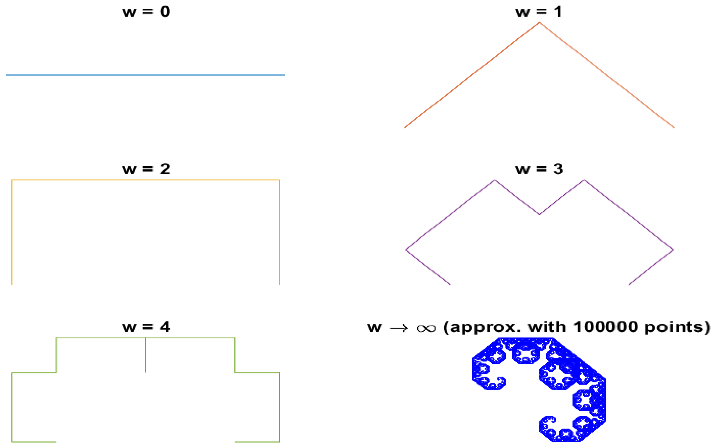
This fractal, characterized by its self-similarity and recursive structure, emerges as the collective limit of the iterated mappings, showcasing the beauty and complexity inherent in fractal geometry. Now, let us explore another fascinating example: the Dragon Curve, a quintessential masterpiece in the domain of fractal geometry. This intricate structure emerges through a captivating interplay of iterative transformations, meticulously orchestrated by affine mappings; ${\mathrm{T}}_1$ and ${\mathrm{T}}_2$ are essential to this process, with each using unique geometric properties to modify the pattern. ${\mathrm{T}}_1$ simply applies the diagonal reflection and scaling, shaping points, particularly with the matrix $\left(\begin{array}{cc}\frac{1}{2}& \frac{-1}{2}\\ \frac{1}{2}& \frac{1}{2}\end{array}\right)$. The mapping ${\mathrm{T}}_2$ adds the reflection and translation using the matrix given by $\left(\begin{array}{cc}\frac{1}{2}& \frac{1}{2}\\ \frac{-1}{2}& \frac{1}{2}\end{array}\right)$, with a shift in $(1,0)$. The combination of these maps results in the wonderful variety of the Dragon Curve fractal. By increasing the iterations, the simple line segments smoothly evolve under their effect, unveiling beautiful patterns that connect across a range of scales. So, the Dragon Curve shows the natural magic and fascinating magnificence that lies in the heart of fractal geometry. The fractal representation of the IFS is shown in Figure 2.

The given IFS is categorized by two mappings ${\mathrm{T}}_1$ and ${\mathrm{T}}_2$. This is a useful tool for producing pseudo-random numbers. By repeating these mappings on some given initial data, the resulting values create properties likely to those of random iterations. However, it is not completely random; this scheme is very useful in many scenarios that seek randomness, such as random sampling techniques, Monte Carlo simulations [35], and algorithms related to cryptography [36]. Monte Carlo simulations are computational methods that employ repeated random sampling to approximate complex mathematical and physical phenomena. They are widely used to model systems with uncertain variables and assess risks, providing valuable insights into areas like finance, engineering, and physics. By producing and examining many random samples, Monte Carlo methods can estimate probabilities and outcomes in cases where analytical solutions are not possible. On the other hand, cryptographic algorithms are developed to protect data through encryption and decryption, ensuring confidentiality, integrity, and authenticity. These algorithms, which encompass both symmetric and asymmetric key methods, are crucial for safeguarding sensitive information and securing digital communications. Moreover, Monte Carlo simulations are employed in cryptography to enhance key generation and validate algorithms, demonstrating their versatile application and importance across different domains. The resulting graph displays the sequence’s progression, developed by the IFS. The development of pseudo-random numbers is core to mathematics and related fields like numerical optimization, simulations, statistical analysis, cryptography, and other computational fields. These pseudo-numbers allow researchers to introduce uncertainty and variability into mathematical models and numerical optimization. This also enables them to study how systems behave under different conditions and make probabilistic predictions. Thus, the application of IFS in the production of pseudo-random numbers is primary in both mathematical research and computational workflows.

In 1969, Nadler [4] generalized the fixed point theorem presented in [3] by replacing the operator from single-valued to multi-valued mapping. We use the following lemma from [4].

Lemma 2

([4]). Suppose $(\mathrm{X},\mathrm{d})$ is a metric space, $\mathcal{X},\mathcal{Z}\subseteq \mathrm{X}$ and $\lambda >1$. Then for each $\mathfrak{x}\in \mathcal{U}$, there exists $\mathfrak{z}\in \mathcal{Z}$, such that we have the following:

$$\mathrm{d}(\mathfrak{x},\mathfrak{z})\le \lambda {\mathfrak{h}}_{\mathfrak{v}}(\mathcal{U},\mathcal{Z}).$$

In 1969, Kannan [37] established a fixed point theorem for Kannan operators, which do not require continuity. A mapping $\mathrm{T}:\mathrm{X}\to \mathrm{X}$ is called a Kannan contraction mapping if $\exists \mathfrak{g}\in [0,\frac{1}{2})$ such that $\forall \eta ,\nu \in \mathrm{X}$, and the following inequality holds:

$$\mathrm{d}(\mathrm{T}\eta ,\mathrm{T}\nu )\le \mathfrak{g}·\left[\mathrm{d}\right(\eta ,\mathrm{T}\eta )+\mathrm{d}(\nu ,\mathrm{T}\nu \left)\right]$$

(2)

This discovery led to more research into contractive-type conditions that do not require the continuity of $\mathrm{T}$. Kannan’s theorem has been generalized in many ways by several authors to extend the scope of the metric fixed point theory in various directions.

Recently, Karapınar [38] expanded the scope of Kannan contraction mappings by developing a new category known as interpolative Kannan-type contraction mappings.

Definition 2

([38]). A mapping $\mathrm{T}:\mathrm{X}\to \mathrm{X}$ is termed an interpolative Kannan-type contraction if there exist $\mathfrak{g}\in [0,1)$ and ${\rm Y}\in (0,1)$ such that the following condition holds:

$$\mathrm{d}(\mathrm{T}\eta ,\mathrm{T}\nu )\le \mathfrak{g}{\left[\mathrm{d}(\eta ,\mathrm{T}\eta )\right]}^{{\rm Y}}{\left[\mathrm{d}(\nu ,\mathrm{T}\nu )\right]}^{1-{\rm Y}},\forall \eta ,\nu \in \mathrm{X}\setminus \mathit{Fix}\left(\mathrm{T}\right),$$

(3)

where $\mathit{Fix}\left(\mathrm{T}\right)=\{\eta \in \mathrm{X}:\eta =\mathrm{T}\eta \}$.

To highlight the constants $\mathfrak{g}$ and ${\rm Y}$ involved in (3), we refer to the interpolative Kannan-type contraction mapping as $(\mathfrak{g},{\rm Y})$–IKC. Reference [38] demonstrated that any interpolative Kannan-type contraction mapping defined on a complete metric space possesses a unique fixed point.

The multi-valued version of the above definition is given as follows:

Definition 3.

A map $\mathrm{T}:\mathrm{X}\to \mathcal{Q}\left(\mathrm{X}\right)$ is called a multi-valued interpolative Kannan-type contraction if $\mathfrak{g}\in [0,1)$ and ${\rm Y}\in (0,1)$ exist, such that the following holds:

$${\mathfrak{h}}_{\mathfrak{v}}(\mathrm{T}\eta ,\mathrm{T}\nu )\le \mathfrak{g}{\left[\mathrm{d}(\eta ,\mathrm{T}\eta )\right]}^{{\rm Y}}{\left[\mathrm{d}(\nu ,\mathrm{T}\nu )\right]}^{1-{\rm Y}},\forall \eta ,\nu \in \mathrm{X}\setminus \mathit{Fix}\left(\mathrm{T}\right),$$

(4)

where $\mathit{Fix}\left(\mathrm{T}\right)=\{\eta \in \mathrm{X}:\eta \in \mathrm{T}\eta \}$.

To highlight the constants involved in Definition (4), we refer to a multi-valued interpolative Kannan-type contraction as $(\mathfrak{g},{\rm Y})$–MIKC.

Not long ago, Sahu et al. [32] demonstrated the IFS on Kannan contraction mappings. They defined the concept of K-IFS by selecting some finite Kannan contractions ${\mathrm{T}}^{\left(w\right)},w=1,2,\cdots , p$ over the complete metric space $(\mathrm{X},\mathrm{d})$, and provided the following result using the famous Collage Theorem:

Theorem 2

([32]) Consider a continuous Y–Kannan mapping $\mathrm{T}:\mathrm{X}\to \mathrm{X}$ on $(\mathrm{X},\mathrm{d})$. Then, for every $\mathcal{Z}\in \mathcal{Q}\left(\mathrm{X}\right)$, the mapping ${\mathrm{T}}^{*}:\mathcal{Q}\left(\mathrm{X}\right)\to \mathcal{Q}\left(\mathrm{X}\right)$, defined as ${\mathrm{T}}^{*}\left(\mathcal{Z}\right)=\{\mathrm{T}\left(\eta \right):\eta \in \mathcal{Z}\}$, is also a Y–Kannan mapping on $(\mathcal{Q}\left(\mathrm{X}\right),{\mathfrak{h}}_{\mathfrak{v}}))$.

Theorem 3

([32]). Consider $\{\mathrm{X};\left({\mathrm{T}}^{\left(0\right)}\right),{\mathrm{T}}^{\left(1\right)},{\mathrm{T}}^{\left(2\right)},\cdots ,{\mathrm{T}}^{\left(p\right)}\}$ a Y–KIFS. Then, the Hutchinson operator $\mathfrak{P}:\mathcal{Q}\left(\mathrm{X}\right)\to \mathcal{Q}\left(\mathrm{X}\right)$ defined by $\mathfrak{P}\left(\mathcal{Z}\right)={\bigcup }_{w=1}^p{\mathrm{T}}^{\left(w\right)}\left(\mathcal{Z}\right)$ for all $\mathcal{Z}\in \mathcal{Q}\left(\mathrm{X}\right)$ is a continuous Y–Kannan mapping on the complete metric space $\left(\mathcal{Q}\right(\mathrm{X}),h(\mathrm{d}\left)\right)$. Its unique fixed point, alternatively referred to as an attractor $\mathcal{U}\in \mathcal{Q}\left(\mathrm{X}\right)$ of the KIFS, satisfies $\mathcal{U}=\mathfrak{P}\left(\mathcal{U}\right)={\bigcup }_{w=1}^p{\mathcal{U}}_w$, and is given by $\mathcal{U}={lim}_{w\to \infty }{\mathfrak{P}}^w\left(\mathcal{Z}\right)$ for any $\mathcal{Z}\in \mathcal{Q}\left(\mathrm{X}\right)$.

Expanding on the previously mentioned findings, Sahu et al. [32] presented their renowned Collage Theorem, a seminal contribution to this field. This theorem is very useful and important in the theory of iterated function systems (IFSs) and Kannan contraction mappings, functioning as a powerful tool used for obtaining the dynamics of intricate systems influenced by these operators.

Theorem 4

([32]). In a complete metric space $(\mathrm{X},\mathrm{d})$, take $\mathcal{Z}$ as a fixed set in $\mathcal{Q}\left(\mathrm{X}\right)$, with $ϵ\ge 0$ and the iterated function system (KIFS) $\{\mathrm{X};{\mathrm{T}}^{\left(1\right)},{\mathrm{T}}^{\left(2\right)},\cdots ,{\mathrm{T}}^{\left(p\right)}\}$, with a contractivity factor Y. If $\mathcal{U}$ is the attractor of the given KIFS and

$${\mathfrak{h}}_{\mathfrak{v}}(\mathcal{Z},\bigcup _{w=1}^p{\mathrm{T}}^{\left(w\right)}\left(\mathcal{Z}\right))\le ϵ,$$

then

$${\mathfrak{h}}_{\mathfrak{v}}(\mathcal{Z},\mathcal{U})\le ϵ(1-{\rm Y})/(1-2{\rm Y}).$$

(5)

This inequality explains the relation between the distance from $\mathcal{Z}$ to $\mathcal{U}$ and the factors Y and ϵ, providing a scale of convergence toward the attractor $\mathcal{U}$.

This study initiates a novel iterated function system and iterated multi-function system, called $\mathcal{IK}$–IFS and $\mathcal{IK}$–IMS, respectively, for interpolative Kannan operators, intended to cover a broader range of mappings. We also present the well-known Collage Theorem in the context of interpolative Kannan contractions. Additionally, we delve into the establishment of the attractor’s well-posedness within the framework of $\mathcal{IK}$–IMS. The Hutchinson operator is based on strict contraction mappings. In many practical scenarios, these mappings may not meet such strict criteria. The interpolative Kannan operator addresses this by allowing for more generalized contraction conditions, thus accommodating a wider range of mappings.

2. Main Results

We begin by stating and proving several propositions that illustrate the relationship between the self-mappings ${\mathrm{T}}^w:\mathrm{X}\to \mathrm{X}$ for $w=1,2,\dots ,p$ and the contraction pair $(\mathfrak{g},{\rm Y})$. Additionally, we will prove the uniqueness of the fixed point of $\mathrm{T}$, if such a fixed point exists.

Proposition 1.

Let $\mathrm{T}:\mathrm{X}\to \mathrm{X}$ be a continuous $(\mathfrak{g},{\rm Y})$–IKC, where $(\mathrm{X},\mathrm{d})$ is a metric space. Then $\mathrm{T}$ satisfies the following expression for all $\eta \in \mathrm{X}$ and $w\in \mathbb{N}$:

$$\mathrm{d}({\mathrm{T}}^w\left(\eta \right),{\mathrm{T}}^{w+1}\left(\eta \right))\le {\mathfrak{g}}^{\frac{1}{{{\rm Y}}^w}}\mathrm{d}(\eta ,\mathrm{T}\eta ).$$

Furthermore, in limiting case

$$\underset{w\to \infty }{lim}\mathrm{d}({\mathrm{T}}^w\left(\eta \right),{\mathrm{T}}^{w+1}\left(\eta \right))=0.$$

Proof. 

By definition of $(\mathfrak{g},{\rm Y})$–IKC, we have the following:

$$\begin{array}{cc}\hfill \mathrm{d}({\mathrm{T}}^w\left(\eta \right),{\mathrm{T}}^{w+1}\left(\eta \right))& =\mathrm{d}(\mathrm{T}\left({\mathrm{T}}^{w-1}\left(\eta \right)\right),\mathrm{T}\left({\mathrm{T}}^w\left(\eta \right)\right))\hfill \\ \hfill & \le \mathfrak{g}\mathrm{d}{({\mathrm{T}}^{w-1}\left(\eta \right),{\mathrm{T}}^w\left(\eta \right))}^{{\rm Y}}\mathrm{d}{({\mathrm{T}}^w\left(\eta \right),{\mathrm{T}}^{w+1}\left(\eta \right))}^{1-{\rm Y}}\hfill \\ \hfill \Rightarrow \mathrm{d}{({\mathrm{T}}^w\left(\eta \right),{\mathrm{T}}^{w+1}\left(\eta \right))}^{{\rm Y}}& \le \mathfrak{g}\mathrm{d}{({\mathrm{T}}^{w-1}\left(\eta \right),{\mathrm{T}}^w\left(\eta \right))}^{{\rm Y}}\hfill \\ \hfill \Rightarrow \mathrm{d}({\mathrm{T}}^w\left(\eta \right),{\mathrm{T}}^{w+1}\left(\eta \right))& \le {\mathfrak{g}}^{\frac{1}{{\rm Y}}}\mathrm{d}({\mathrm{T}}^{w-1}\left(\eta \right),{\mathrm{T}}^w\left(\eta \right))\hfill \\ \hfill & \le {\mathfrak{g}}^{\frac{1}{{\rm Y}}}{\mathfrak{g}}^{\frac{1}{{\rm Y}}}\mathrm{d}({\mathrm{T}}^{w-2}\left(\eta \right),{\mathrm{T}}^{w-1}\left(\eta \right))\hfill \\ \hfill & ={\mathfrak{g}}^{\frac{1}{{{\rm Y}}^2}}\mathrm{d}({\mathrm{T}}^{w-2}\left(\eta \right),{\mathrm{T}}^{w-1}\left(\eta \right))\hfill \\ \hfill & ⋮\hfill \\ \hfill \Rightarrow \mathrm{d}({\mathrm{T}}^w\left(\eta \right),{\mathrm{T}}^{w+1}\left(\eta \right))& \le {\mathfrak{g}}^{\frac{1}{{{\rm Y}}^w}}\mathrm{d}(x,\mathrm{T}\left(\eta \right)).\hfill \end{array}$$

In the limiting case, we obtain the following:

$$\underset{w\to \infty }{lim}\mathrm{d}({\mathrm{T}}^w\left(\eta \right),{\mathrm{T}}^{w+1}\left(\eta \right))=0,$$

since ${\mathfrak{g}}^{\frac{1}{{{\rm Y}}^w}}\to 0$ as $w\to \infty$. □

Subsequently, we present the following findings, where we prove that each continuous interpolative Kannan operator on a complete metric space must satisfy the inequality (6).

Proposition 2.

Let $\mathrm{T}:\mathrm{X}\to \mathrm{X}$ be a continuous $(\mathfrak{g},{\rm Y})$–IKC on the complete metric space $(\mathrm{X},\mathrm{d})$, and ${\eta }^{*}\in Fix\left(\mathrm{T}\right)$. Then, we have the following:

$$\mathrm{d}(\eta ,{\eta }^{*})\le \frac{1}{1-{\mathfrak{g}}^{\frac{1}{{{\rm Y}}^w}}}\mathrm{d}(\eta ,\mathrm{T}\eta ),\forall \eta \in \mathrm{X}.$$

(6)

Proof. 

Since ${\eta }^{*}\in Fix\left(\mathrm{T}\right)$, we have $\forall \eta \in \mathrm{X}$ and ${lim}_{w\to \infty }{\mathrm{T}}^w\left(\eta \right)={\eta }^{*}.$ By using the continuity of $\mathrm{T}$, the triangular inequality, and Proposition 1, we obtain the following:

$$\begin{array}{ccc}\hfill \mathrm{d}(\eta ,{\eta }^{*})& =& \mathrm{d}(\eta ,\underset{w\to \infty }{lim}{\mathrm{T}}^w(\eta ))\hfill \\ & =& \underset{w\to \infty }{lim}\mathrm{d}(\eta ,{\mathrm{T}}^w\left(\eta \right))\hfill \\ & \le & {\displaystyle \underset{w\to \infty }{lim}}{\displaystyle \sum _{m=1}^w}\mathrm{d}({\mathrm{T}}^{m-1}\left(\eta \right),{\mathrm{T}}^m\left(\eta \right))\hfill \\ & \le & \underset{w\to \infty }{lim}(1+{\mathfrak{g}}^{\frac{1}{{\rm Y}}}+{\mathfrak{g}}^{\frac{1}{{{\rm Y}}^2}}+\cdots +{\mathfrak{g}}^{\frac{1}{{{\rm Y}}^{w-1}}})\mathrm{d}(\eta ,\mathrm{T}\eta )\hfill \\ & \le & (1+{\mathfrak{g}}^{\frac{1}{{\rm Y}}}+{\mathfrak{g}}^{\frac{1}{{{\rm Y}}^2}}+\cdots )\mathrm{d}(\eta ,\mathrm{T}\eta )\hfill \\ & =& \frac{1}{1-{\mathfrak{g}}^{\frac{1}{{\rm Y}}}}\mathrm{d}(\eta ,\mathrm{T}\eta ).\hfill \end{array}$$

□

Next, we state and prove the following lemma, which plays a crucial role in our main findings:

Lemma 3.

If η, $\mathfrak{b}$, $\mathfrak{c}$, and $\mathfrak{d}$ are non-negative real numbers, then we have the following:

$$max\{\eta ·\mathfrak{b},\mathfrak{c}·\mathfrak{d}\}\le max\{\eta ,\mathfrak{c}\}·max\{\mathfrak{b},\mathfrak{d}\}.$$

Proof. 

To prove that $max\{\eta ·\mathfrak{b},\mathfrak{c}·\mathfrak{d}\}\le max\{\eta ,\mathfrak{c}\}·max\{\mathfrak{b},\mathfrak{d}\}$, where $\eta ,\mathfrak{b},\mathfrak{c},$ and $\mathfrak{d}$ are non-negative real numbers, we use case analysis based on the values of $\eta ,\mathfrak{b},\mathfrak{c},$ and $\mathfrak{d}$. Let ${\mathfrak{M}}_1=max\{\eta ·\mathfrak{b},\mathfrak{c}·\mathfrak{d}\}$ and ${\mathfrak{M}}_2=max\{\eta ,\mathfrak{c}\}·max\{\mathfrak{b},\mathfrak{d}\}$. We need to analyze the maximum values in two steps: first for the pairs $\{\eta ,\mathfrak{c}\}$ and $\{\mathfrak{b},\mathfrak{d}\}$, and then for the products $\eta ·\mathfrak{b}$ and $\mathfrak{c}·\mathfrak{d}$.

• Case 1: $\eta \ge \mathfrak{c}$ and $\mathfrak{b}\ge \mathfrak{d}$
  In this case, $max\{\eta ,\mathfrak{c}\}=\eta$ and $max\{\mathfrak{b},\mathfrak{d}\}=\mathfrak{b}$. So, ${\mathfrak{M}}_2=\eta ·\mathfrak{b}$. Since $\eta ·\mathfrak{b}$ is one of the elements being compared in ${\mathfrak{M}}_1$. Therefore, $max\{\eta ·\mathfrak{b},\mathfrak{c}·\mathfrak{d}\}\le \eta ·\mathfrak{b}$ and, hence, ${\mathfrak{M}}_1\le {\mathfrak{M}}_2$.
• Case 2: $\eta \ge \mathfrak{c}$ and $\mathfrak{b}<\mathfrak{d}$
  In this case, $max\{\eta ,\mathfrak{c}\}=\eta$ and $max\{\mathfrak{b},\mathfrak{d}\}=\mathfrak{d}$. So, ${\mathfrak{M}}_2=\eta ·\mathfrak{d}$. Since $\eta ·\mathfrak{b}\le \eta ·\mathfrak{d}$ (because $\mathfrak{b}\le \mathfrak{d}$) and $\mathfrak{c}·\mathfrak{d}\le \eta ·\mathfrak{d}$ (because $\mathfrak{c}\le \eta$). Therefore, $max\{\eta ·\mathfrak{b},\mathfrak{c}·\mathfrak{d}\}\le \eta ·\mathfrak{d}$ and, hence, ${\mathfrak{M}}_1\le {\mathfrak{M}}_2$.
• Case 3: $\eta <\mathfrak{c}$ and $\mathfrak{b}\ge \mathfrak{d}$
  In this case, $max\{\eta ,\mathfrak{c}\}=\mathfrak{c}$ and $max\{\mathfrak{b},\mathfrak{d}\}=\mathfrak{b}$. So, ${\mathfrak{M}}_2=\mathfrak{c}·\mathfrak{b}$. Since $\eta ·\mathfrak{b}\le \mathfrak{c}·\mathfrak{b}$ (because $\eta \le \mathfrak{c}$) and $\mathfrak{c}·\mathfrak{d}\le \mathfrak{c}·\mathfrak{b}$ (because $\mathfrak{d}\le \mathfrak{b}$). Therefore, $max\{\eta ·\mathfrak{b},\mathfrak{c}·\mathfrak{d}\}\le \mathfrak{c}·\mathfrak{b}$ and, hence, ${\mathfrak{M}}_1\le {\mathfrak{M}}_2$.
• Case 4: $\eta <\mathfrak{c}$ and $\mathfrak{b}<\mathfrak{d}$
  In this case, $max\{\eta ,\mathfrak{c}\}=\mathfrak{c}$ and $max\{\mathfrak{b},\mathfrak{d}\}=\mathfrak{d}$. So, ${\mathfrak{M}}_2=\mathfrak{c}·\mathfrak{d}$. Since $\eta ·\mathfrak{b}\le \mathfrak{c}·\mathfrak{d}$ and $\mathfrak{c}·\mathfrak{d}=\mathfrak{c}·\mathfrak{d}$. Therefore, $max\{\eta ·\mathfrak{b},\mathfrak{c}·\mathfrak{d}\}\le \mathfrak{c}·\mathfrak{d}$ and, hence, ${\mathfrak{M}}_1\le {\mathfrak{M}}_2$.

Hence, in all cases, we show the following:

$$max\{\eta ·\mathfrak{b},\mathfrak{c}·\mathfrak{d}\}\le max\{\eta ,\mathfrak{c}\}·max\{\mathfrak{b},\mathfrak{d}\}.$$

Thus, the inequality is proven for all non-negative real numbers $\eta ,\mathfrak{b},\mathfrak{c},$ and $\mathfrak{d}$. □

Next, we generalize the above lemma for the case of finite numbers as follows:

Lemma 4.

For any non-negative real numbers $\left({\eta }_w\right)$, $\left({\mathfrak{b}}_w\right)$, where $w=1,2,\cdots ,p$, the following inequality holds:

$$max\{{\Pi }_{w=1}^p{\eta }_w,{\Pi }_{w=1}^p{\mathfrak{b}}_w\}\le {\Pi }_{w=1}^{p}max\{{\eta }_w,{\mathfrak{b}}_w\}.$$

Proof. 

The proof of this lemma is straightforward and can be derived using Lemma 3. □

Next, we define the interpolative Kannan iteration function system as well as the iteration multi-function system, which involves the use of interpolative Kannan contraction operators. The traditional Hutchinson operator depends on strict contraction mappings. However, in many practical scenarios, these mappings may not strictly meet these conditions. The interpolative Kannan operator relaxes these requirements, accommodating mappings that satisfy more generalized contraction conditions.

Definition 4.

Let $(\mathrm{X},\mathrm{d})$ be a metric space and $\{{\mathrm{T}}^{\left(w\right)}:\mathrm{X}\to \mathrm{X},w=1,2,\cdots ,p\}$ be a finite collection of interpolative Kannan contraction operators (IKCs) with contraction pair $({\mathfrak{g}}_w,{{\rm Y}}_w),\forall w=1,2,\cdots ,p$. Then, we call $(\mathrm{X};{\mathrm{T}}^{\left(w\right)},w=1,2,\cdots ,p)$, a $({\mathfrak{g}}_w,{{\rm Y}}_w)$–IKC-IFS or simply IKC-IFS.

Similarly, the IMS for the multi-valued interpolative Kannan contraction operators is defined as follows:

Definition 5.

Suppose $(\mathrm{X},\mathrm{d})$ is a metric space and $\{{\mathrm{T}}^{\left(w\right)}:\mathrm{X}\to \mathcal{Q}\left(\mathrm{X}\right),w=1,2,\cdots ,p\}$ is a finite collection of multi-valued interpolative Kannan contraction operators (MIKCs) with the contraction pair $({\mathfrak{g}}_w,{{\rm Y}}_w),\forall w=1,2,\cdots ,p$. Then, we call $(\mathrm{X};{\mathrm{T}}^{\left(w\right)},w=1,2,\cdots ,p)$, a $({\mathfrak{g}}_w,{{\rm Y}}_w)$–IKC-IMS.

Our initial result is as follows. This outcome presents the initial findings and sets the stage for further analysis.

Theorem 5.

Let $\mathrm{T}:\mathrm{X}\to \mathrm{X}$ be a continuous $(\mathfrak{g},{\rm Y})$–IKC. Then ${\mathrm{T}}^{*}$ is defined by ${\mathrm{T}}^{*}\left(\mathcal{U}\right)=\{\mathrm{T}\left(\eta \right);\eta \in \mathcal{U}\}$, $\forall \mathcal{U}\in \mathcal{Q}\left(\mathrm{X}\right)$, and maps $\mathcal{Q}\left(\mathrm{X}\right)$ into itself, and ${\mathrm{T}}^{*}$ is also a $(\mathfrak{g},{\rm Y})$–IKC on $(\mathcal{Q}\left(\mathrm{X}\right),{\mathfrak{h}}_{\mathfrak{v}})$.

Proof. 

Since $\mathrm{T}$ is continuous mapping, then ${\mathrm{T}}^{*}$ maps compact subsets of $\mathrm{X}$ into compact subsets of $\mathrm{X}$. That is, ${\mathrm{T}}^{*}$ maps $\mathcal{Q}\left(\mathrm{X}\right)$ into itself.

Secondly, we have the following:

$$\begin{array}{ccc}\hfill D(\mathrm{T}\eta ,\mathrm{T}\mathcal{Z})& =& {\displaystyle \underset{\nu \in B\mathcal{Z}}{inf}}\left\{\mathrm{d}(\mathrm{T}\eta ,\mathrm{T}\nu )\right\}\hfill \\ & \le & {\displaystyle \underset{\nu \in \mathcal{Z}}{inf}}\left\{\mathfrak{g}\mathrm{d}{(\eta ,\mathrm{T}\eta )}^{{\rm Y}}\mathrm{d}{(\nu ,\mathrm{T}\nu )}^{1-{\rm Y}}\right\}\hfill \\ & \le & \mathfrak{g}\mathrm{d}{(\eta ,\mathrm{T}\eta )}^{{\rm Y}}{\mathfrak{h}}_{\mathfrak{v}}{(\mathcal{Z},\mathrm{T}\mathcal{Z})}^{1-{\rm Y}}.\hfill \end{array}$$

(7)

Similarly,

$$\begin{array}{ccc}\hfill D(\mathrm{T}\nu ,\mathrm{T}\mathcal{U})& =& {\displaystyle \underset{\eta \in \mathcal{U}}{inf}}\left\{\mathrm{d}(\mathrm{T}\nu ,\mathrm{T}\eta )\right\}\hfill \\ & \le & \underset{\eta \in \mathcal{U}}{inf}\left\{\mathfrak{g}\mathrm{d}{(\nu ,\mathrm{T}\nu )}^{{\rm Y}}\mathrm{d}{(\eta ,\mathrm{T}\eta )}^{1-{\rm Y}}\right\}\hfill \\ & \le & \mathfrak{g}\mathrm{d}{(\nu ,\mathrm{T}\nu )}^{{\rm Y}}{\mathfrak{h}}_{\mathfrak{v}}{(\mathcal{U},\mathrm{T}\mathcal{U})}^{1-{\rm Y}}.\hfill \end{array}$$

(8)

Thus, using (7) and (8), we obtain the following:

$$\begin{array}{ccc}\hfill {\mathfrak{h}}_{\mathfrak{v}}(\mathrm{T}\mathcal{U},\mathrm{T}\mathcal{Z})& =& max\{\underset{\eta \in \mathcal{U}}{sup}D(\mathrm{T}\eta ,\mathrm{T}\mathcal{Z}),\underset{\nu \in \mathcal{Z}}{sup}D(\mathrm{T}\nu ,\mathrm{T}\mathcal{U})\}\hfill \\ & \le & max\{\underset{\eta \in \mathcal{U}}{sup}\mathfrak{g}\mathrm{d}{(\eta ,\mathrm{T}\eta )}^{{\rm Y}}{\mathfrak{h}}_{\mathfrak{v}}{(\mathcal{Z},\mathrm{T}\mathcal{Z})}^{1-{\rm Y}},\underset{\nu \in \mathcal{Z}}{sup}\mathfrak{g}\mathrm{d}{(\nu ,\mathrm{T}\nu )}^{{\rm Y}}{\mathfrak{h}}_{\mathfrak{v}}{(\mathcal{U},\mathrm{T}\mathcal{U})}^{1-{\rm Y}}\}\hfill \\ & =& \mathfrak{g}·{\mathfrak{h}}_{\mathfrak{v}}{(\mathcal{U},\mathrm{T}\mathcal{U})}^{{\rm Y}}{\mathfrak{h}}_{\mathfrak{v}}{(\mathcal{Z},\mathrm{T}\mathcal{Z})}^{1-{\rm Y}}.\hfill \end{array}$$

This shows that ${\mathrm{T}}^{*}$ is also a $(\mathfrak{g},{\rm Y})$–IKC. □

We define the Hutchinson operator and Hutchinson-like operator equipped with interpolative Kannan mappings as follows:

Definition 6.

Consider $(\mathrm{X},\mathrm{d})$ be a metric space and $\left\{{\mathrm{T}}^{\left(w\right)}\right\}$, where $w=1,2,\cdots ,p$, be a finite collection of $({\mathfrak{g}}_w,{{\rm Y}}_w)$–IKCs. Then the transformation $\mathfrak{P}:\mathcal{Q}\left(\mathrm{X}\right)\to \mathcal{Q}\left(\mathrm{X}\right)$ is defined by the following:

$$\mathfrak{P}\left(\mathcal{Z}\right)=\bigcup _{w=1}^p{\mathrm{T}}^{\left(w\right)}\left(\mathcal{Z}\right),\forall \mathcal{Z}\in \mathcal{Q}\left(\mathrm{X}\right),$$

(9)

and is called the Hutchinson operator equipped with IKCs.

Definition 7.

Let $(\mathrm{X},\mathrm{d})$ be a metric space and $\left\{{\mathrm{T}}^{\left(w\right)}\right\}$, where $w=1,2,\cdots ,p$ is a finite collection of $({\mathfrak{g}}_w,{{\rm Y}}_w)$–MIKCs. Then the transformation $\mathfrak{P}:\mathrm{X}\to \mathcal{Q}\left(\mathrm{X}\right)$ is defined by the following:

$$\mathfrak{P}\left(\mathfrak{z}\right)=\bigcup _{w=1}^p{\mathrm{T}}^{\left(w\right)}\left(\mathfrak{z}\right),\forall \mathfrak{z}\in \mathrm{X},$$

(10)

and is called the Hutchinson-like operator associated with MIKCs.

In the following, we present some results about the Hutchinson operator formed by the interpolative Kannan operators.

Theorem 6.

Suppose $(\mathrm{X},\mathrm{d})$ is a metric space and $\left\{{\mathrm{T}}^{\left(w\right)}\right\}$, where $w=1,2,\cdots ,p$ is a finite collection of $({\mathfrak{g}}_w,{{\rm Y}}_w)$–IKCs. Then the transformation $\mathfrak{P}:\mathcal{Q}\left(\mathrm{X}\right)\to \mathcal{Q}\left(\mathrm{X}\right)$ is given by the following:

$$\mathfrak{P}\left(\mathcal{U}\right)=\bigcup _{w=1}^p{\mathrm{T}}^{\left(w\right)}\left(\mathcal{U}\right),\forall \mathcal{U}\in \mathcal{Q}\left(\mathrm{X}\right),$$

(11)

is also a $(\mathfrak{g},{\rm Y})$–IKC on $(\mathcal{Q}\left(\mathrm{X}\right),{\mathfrak{h}}_{\mathfrak{v}})$, with $\mathfrak{g}={max}_{w=1}^p{\mathfrak{g}}_w$ and ${\rm Y}={max}_{w=1}^p{{\rm Y}}_w$.

Proof. 

Consider the following in light of Lemma 1 and Lemma 4:

$$\begin{array}{ccc}\hfill {\mathfrak{h}}_{\mathfrak{v}}(\mathfrak{P}\left(\mathcal{U}\right),\mathfrak{P}\left(\mathcal{Z}\right))& =& {\mathfrak{h}}_{\mathfrak{v}}({\displaystyle \bigcup _{w=1}^p}{\mathrm{T}}^{\left(w\right)}\left(\mathcal{U}\right),{\displaystyle \bigcup _{w=1}^p}{\mathrm{T}}^{\left(w\right)}\left(\mathcal{Z}\right))\hfill \\ & \le & \underset{w=1}{\overset{p}{max}}{\mathfrak{h}}_{\mathfrak{v}}({\mathrm{T}}^{\left(w\right)}\left(\mathcal{U}\right),{\mathrm{T}}^{\left(w\right)}\left(\mathcal{Z}\right))\hfill \\ & \le & \underset{w=1}{\overset{p}{max}}{\mathfrak{g}}_w·{\mathfrak{h}}_{\mathfrak{v}}{(\mathcal{U},{\mathrm{T}}^{\left(w\right)}\left(\mathcal{U}\right))}^{{{\rm Y}}_w}{\mathfrak{h}}_{\mathfrak{v}}{(\mathcal{Z},{\mathrm{T}}^{\left(w\right)}\left(\mathcal{Z}\right))}^{1-{{\rm Y}}_w}\hfill \\ & \le & \mathfrak{g}·\underset{w=1}{\overset{p}{max}}{\mathfrak{h}}_{\mathfrak{v}}{(\mathcal{U},{\mathrm{T}}^{\left(w\right)}\left(\mathcal{U}\right))}^{{\rm Y}}{\mathfrak{h}}_{\mathfrak{v}}{(\mathcal{Z},{\mathrm{T}}^{\left(w\right)}\left(\mathcal{Z}\right))}^{1-{\rm Y}},\hfill \\ & (\mathrm{where}& \mathfrak{g}=\underset{w=1}{\overset{p}{max}}{\mathfrak{g}}_w\&{\rm Y}=\underset{w=1}{\overset{p}{max}}{{\rm Y}}_w)\hfill \\ & \le & \mathfrak{g}·\Pi \underset{w=1}{\overset{p}{max}}\left\{{\mathfrak{h}}_{\mathfrak{v}}{(\mathcal{U},{\mathrm{T}}^{\left(w\right)}\left(\mathcal{U}\right))}^{{\rm Y}},{\mathfrak{h}}_{\mathfrak{v}}{(\mathcal{Z},{\mathrm{T}}^{\left(w\right)}\left(\mathcal{Z}\right))}^{1-{\rm Y}}\right\}\hfill \\ & =& \mathfrak{g}·\Pi \{{\mathfrak{h}}_{\mathfrak{v}}{(\mathcal{U},{\displaystyle \bigcup _{w=1}^p}{\mathrm{T}}^{\left(w\right)}\left(\mathcal{U}\right))}^{{\rm Y}},{\mathfrak{h}}_{\mathfrak{v}}{(\mathcal{Z},{\displaystyle \bigcup _{w=1}^p}{\mathrm{T}}^{\left(w\right)}\left(\mathcal{Z}\right))}^{1-{\rm Y}}\}\hfill \\ & =& \mathfrak{g}·{\mathfrak{h}}_{\mathfrak{v}}{(\mathcal{U},{\displaystyle \bigcup _{w=1}^p}{\mathrm{T}}^{\left(w\right)}\left(\mathcal{U}\right))}^{{\rm Y}}·{\mathfrak{h}}_{\mathfrak{v}}{(\mathcal{Z},{\displaystyle \bigcup _{w=1}^p}{\mathrm{T}}^{\left(w\right)}\left(\mathcal{Z}\right))}^{1-{\rm Y}}\hfill \\ & =& \mathfrak{g}·{\mathfrak{h}}_{\mathfrak{v}}{(\mathcal{U},\mathfrak{P}\left(\mathcal{U}\right))}^{{\rm Y}}·{\mathfrak{h}}_{\mathfrak{v}}{(\mathcal{Z},\mathfrak{P}\left(\mathcal{Z}\right))}^{1-{\rm Y}}.\hfill \end{array}$$

Thus, $\mathfrak{P}$ is also a $(\mathfrak{g},{\rm Y})$–IKC, where $\mathfrak{g}={max}_{w=1}^p{\mathfrak{g}}_w\&{\rm Y}={max}_{w=1}^p{{\rm Y}}_w$. □

The Hutchinson operator—equipped with interpolative Kannan contractions—is also a Kannan contraction. So, we simply call it the $(\mathfrak{g},{\rm Y})$–IKC–Hutchinson operator, where $\mathfrak{g}={max}_{w=1}^p{\mathfrak{g}}_w$ and ${\rm Y}={max}_{w=1}^p{{\rm Y}}_w$.

Theorem 7.

Consider the $({\mathfrak{g}}_w,{{\rm Y}}_w)$–IKC-IFS $(\mathrm{X};{\mathrm{T}}^{\left(w\right)},1,2,\cdots ,p)$ on a complete metric space $(\mathrm{X},\mathrm{d})$ and the $(\mathfrak{g},{\rm Y})$–IKC $\mathfrak{P}:\mathcal{Q}\left(\mathrm{X}\right)\to \mathcal{Q}\left(\mathrm{X}\right)$ defined by $\mathfrak{P}\left(\mathcal{U}\right)={\bigcup }_{w=1}^p{\mathrm{T}}^{\left(w\right)}\left(\mathcal{U}\right),\forall \mathcal{U}\in \mathcal{Q}\left(\mathrm{X}\right),$ where $\mathfrak{g}={max}_{w=1}^p{\mathfrak{g}}_w\&{\rm Y}={max}_{w=1}^p{{\rm Y}}_w$. Then, $\mathfrak{P}$ has a unique attractor of the given IFS, say ${\mathcal{U}}^{*}\in \mathcal{Q}\left(\mathrm{X}\right)$, satisfying $A^{*}=\mathfrak{P}\left({\mathcal{U}}^{*}\right)={\bigcup }_{w=1}^p{\mathrm{T}}^{\left(w\right)}\left({\mathcal{U}}^{*}\right)$, and is given by ${\mathcal{U}}^{*}={lim}_{w\to \infty }{\mathfrak{P}}^w\left(\mathcal{Z}\right)$ for any initial choice of $\mathcal{Z}\in \mathcal{Q}\left(\mathrm{X}\right)$.

Proof. 

Let ${\mathcal{U}}_0\in \mathcal{Q}\left(\mathrm{X}\right)$ be any arbitrary point and establish the sequence ${\mathcal{U}}_{w+1}=\mathfrak{P}\left({\mathcal{U}}_w\right),\forall w\in \mathbb{N}$. By using Theorem (6), it is clear that $\mathfrak{P}$ is a $(\mathfrak{g},{\rm Y})$–IKC, where $\mathfrak{g}={max}_{w=1}^p{\mathfrak{g}}_w\&{\rm Y}={max}_{w=1}^p{{\rm Y}}_w$. Then, we have the following:

$$\begin{array}{ccc}\hfill {\mathfrak{h}}_{\mathfrak{v}}({\mathcal{U}}_w,{\mathcal{U}}_{w+1})& =& {\mathfrak{h}}_{\mathfrak{v}}(\mathfrak{P}\left({\mathcal{U}}_{w-1}\right),\mathfrak{P}\left({\mathcal{U}}_w\right))\hfill \\ & \le & \mathfrak{g}·{\mathfrak{h}}_{\mathfrak{v}}{({\mathcal{U}}_{w-1},{\mathcal{U}}_w)}^{{\rm Y}}{\mathfrak{h}}_{\mathfrak{v}}{({\mathcal{U}}_w,{\mathcal{U}}_{w+1})}^{1-{\rm Y}}\hfill \\ \hfill \Rightarrow {\mathfrak{h}}_{\mathfrak{v}}{({\mathcal{U}}_w,{\mathcal{U}}_{w+1})}^{{\rm Y}}& \le & \mathfrak{g}·{({\mathcal{U}}_{\mathfrak{h}}\mathfrak{v}w-1,{\mathcal{U}}_w)}^{{\rm Y}}\hfill \\ \hfill \Rightarrow {\mathfrak{h}}_{\mathfrak{v}}({\mathcal{U}}_w,{\mathcal{U}}_{w+1})& \le & {\mathfrak{g}}^{\frac{1}{{\rm Y}}}·{\mathfrak{h}}_{\mathfrak{v}}({\mathcal{U}}_{w-1},{\mathcal{U}}_w)\hfill \\ & \le & {\mathfrak{g}}^{\frac{1}{{\rm Y}}}·{\mathfrak{g}}^{\frac{1}{{\rm Y}}}·{\mathfrak{h}}_{\mathfrak{v}}({\mathcal{U}}_{w-2},{\mathcal{U}}_{w-1})\hfill \\ & =& {\mathfrak{g}}^{\frac{1}{{{\rm Y}}^2}}·{\mathfrak{h}}_{\mathfrak{v}}({\mathcal{U}}_{w-2},{\mathcal{U}}_{w-1})\hfill \\ & ⋮& \\ \hfill {\mathfrak{h}}_{\mathfrak{v}}({\mathcal{U}}_w,{\mathcal{U}}_{w+1})& \le & {\mathfrak{g}}^{\frac{1}{{{\rm Y}}^w}}·{\mathfrak{h}}_{\mathfrak{v}}({\mathcal{U}}_0,{\mathcal{U}}_1).\hfill \end{array}$$

Letting $w\to \infty$, we obtain ${lim}_{w\to \infty }{\mathfrak{h}}_{\mathfrak{v}}({\mathcal{U}}_w,{\mathcal{U}}_{w+1})=0$.

Next, we show that ${\left\{{\mathcal{U}}_w\right\}}_{w=0}^{\infty }$ is a Cauchy sequence in $(\mathcal{Q}\left(\mathrm{X}\right),{\mathfrak{h}}_{\mathfrak{v}})$. More precisely, for $r>w$, we obtain the following:

$$\begin{array}{ccc}\hfill {\mathfrak{h}}_{\mathfrak{v}}({\mathcal{U}}_w,{\mathcal{U}}_{w+r})& =& {\mathfrak{h}}_{\mathfrak{v}}({\mathcal{U}}_w,{\mathcal{U}}_{w+1})+{\mathfrak{h}}_{\mathfrak{v}}({\mathcal{U}}_{w+1},{\mathcal{U}}_{w+2})+\cdots +{\mathfrak{h}}_{\mathfrak{v}}({\mathcal{U}}_{w+r-1},{\mathcal{U}}_{w+r})\hfill \\ & \le & ({\mathfrak{g}}^{\frac{1}{{{\rm Y}}^w}}+{\mathfrak{g}}^{\frac{1}{{{\rm Y}}^{w+1}}}+\cdots +{\mathfrak{g}}^{\frac{1}{{{\rm Y}}^{w+r-1}}})·{\mathfrak{h}}_{\mathfrak{v}}({\mathcal{U}}_0,{\mathcal{U}}_1)\hfill \\ & \le & ({\mathfrak{g}}^{\frac{1}{{{\rm Y}}^w}}+{\mathfrak{g}}^{\frac{1}{{{\rm Y}}^{w+1}}}+\cdots )·{\mathfrak{h}}_{\mathfrak{v}}({\mathcal{U}}_0,{\mathcal{U}}_1)\hfill \\ & =& \frac{{\mathfrak{g}}^{\frac{1}{{{\rm Y}}^w}}}{1-{\mathfrak{g}}^{\frac{1}{{\rm Y}}}}·{\mathfrak{h}}_{\mathfrak{v}}({\mathcal{U}}_0,{\mathcal{U}}_1)\to 0\mathrm{as}w\to \infty .\hfill \end{array}$$

This implies that $\left\{{\mathcal{U}}_w\right\}$ is a Cauchy sequence and due to the completeness of $\mathcal{Q}\left(\mathrm{X}\right)$, we can find ${\mathcal{U}}^{*}\in \mathcal{Q}\left(\mathrm{X}\right)$ such that ${\mathcal{U}}_w\to {\mathcal{U}}^{*}$ as $w\to \infty$.

Next, we show that ${\mathcal{U}}^{*}\in Fix\left(\mathfrak{P}\right)$. Using the definition of $(\mathfrak{g},{\rm Y})$–IKC, we have the following:

$$\begin{array}{ccc}\hfill {\mathfrak{h}}_{\mathfrak{v}}({\mathcal{U}}_{w+1},\mathfrak{P}\left({\mathcal{U}}^{*}\right))& =& {\mathfrak{h}}_{\mathfrak{v}}(\mathfrak{P}\left({\mathcal{U}}_w\right),\mathfrak{P}\left({\mathcal{U}}^{*}\right))\hfill \\ & \le & \mathfrak{g}·{\mathfrak{h}}_{\mathfrak{v}}{({\mathcal{U}}_w,\mathfrak{P}\left({\mathcal{U}}_w\right))}^{{\rm Y}}{\mathfrak{h}}_{\mathfrak{v}}{({\mathcal{U}}^{*},\mathfrak{P}\left({\mathcal{U}}^{*}\right))}^{1-{\rm Y}}.\hfill \end{array}$$

Taking $w\to \infty$, we obtain ${\mathfrak{h}}_{\mathfrak{v}}({\mathcal{U}}^{*},\mathfrak{P}\left({\mathcal{U}}^{*}\right))=0$, which yields ${\mathcal{U}}^{*}\in Fix\left(\mathfrak{P}\right)$, and ${\mathcal{U}}^{*}$ is an attractor of the $\mathcal{IK}$–IFS. To show the uniqueness of the attractor, take contrary $\mathcal{U},\mathcal{Z}\in Fix\left(\mathfrak{P}\right)$ with $\mathcal{U}\ne \mathcal{Z}$. Then, by definition, we have the following:

$$\begin{array}{ccc}\hfill {\mathfrak{h}}_{\mathfrak{v}}(\mathcal{U},\mathcal{Z})& =& {\mathfrak{h}}_{\mathfrak{v}}(\mathfrak{P}\left(\mathcal{U}\right),\mathfrak{P}\left(\mathcal{Z}\right))\hfill \\ & \le & \mathfrak{g}·{\mathfrak{h}}_{\mathfrak{v}}{(\mathcal{U},\mathfrak{P}\left(\mathcal{U}\right))}^{{\rm Y}}{\mathfrak{h}}_{\mathfrak{v}}{(\mathcal{Z},\mathfrak{P}\left(\mathcal{Z}\right))}^{1-{\rm Y}}\hfill \\ & =& \mathfrak{g}·{\mathfrak{h}}_{\mathfrak{v}}{(\mathcal{U},\mathcal{U})}^{{\rm Y}}{\mathfrak{h}}_{\mathfrak{v}}{(\mathcal{Z},\mathcal{Z})}^{1-{\rm Y}}\hfill \\ \hfill \Rightarrow {\mathfrak{h}}_{\mathfrak{v}}(\mathcal{U},\mathcal{Z})& =& 0.\hfill \end{array}$$

A contradiction. Hence, the fixed point of $\mathfrak{P}$ or the attractor of the $\mathcal{IK}$–IFS is unique. □

Example 1.

Consider a system of two operators defined by the following:

$${\mathrm{T}}^{\left(1\right)}\left(\eta \right)=\left\{\begin{array}{c}0,\mathrm{if}\eta \in [0,2)\hfill \\ \eta +2\mathrm{if}\eta \ge 2\hfill \end{array}\right.$$

and

$${\mathrm{T}}^{\left(2\right)}\left(\eta \right)=\left\{\begin{array}{c}0,\mathrm{if}\eta \in [0,3)\hfill \\ \eta +3,\mathrm{if}\eta \ge 3\hfill \end{array}\right.$$

on $\mathrm{X}=[0,\infty )$ with the usual metric. Suppose that both operators ${\mathrm{T}}^{\left(1\right)}$ and ${\mathrm{T}}^{\left(2\right)}$ are Kannan contractions, satisfying the Kannan inequality (2). First, check ${\mathrm{T}}^{\left(1\right)}$ with $\eta =0$ and $\mathfrak{x}=2$. Then, $\mathrm{d}({\mathrm{T}}^{\left(1\right)}0,{\mathrm{T}}^{\left(1\right)}2)=\mathrm{d}(0,4)=4,\mathrm{d}(0,{\mathrm{T}}^{\left(1\right)}0)=\mathrm{d}(0,0)=0$ and $\mathrm{d}(2,{\mathrm{T}}^{\left(1\right)}2)=\mathrm{d}(2,4)=2$. For some $\mathfrak{g}\in \left[0,\frac{1}{2}\right)$, inequality (2) implies the following:

$$4\le \mathfrak{g}[0+2]\Rightarrow \mathfrak{g}\ge 2.$$

This leads to a contradiction, so ${\mathrm{T}}^{\left(1\right)}$ is not a Kannan mapping. A similar argument can be applied to ${\mathrm{T}}^{\left(2\right)}$ by choosing $\eta =0$ and $\mathfrak{x}=3$. It is evident that both ${\mathrm{T}}^{\left(1\right)}$ and ${\mathrm{T}}^{\left(2\right)}$ satisfy inequality (3) with $\mathfrak{g}=\frac{1}{4}$ and ${\rm Y}=\frac{1}{4}$. Hence, this forms an interpolative iterated function system (IKC-IFS). Consequently, the results provided by Sahu et al. [32] cannot be applied to this example. On the other hand, the corresponding $(\frac{1}{4},\frac{1}{4})$–IKC–Hutchinson-like operator is defined by the following:

$$\mathfrak{P}\left(\mathfrak{z}\right)={\mathrm{T}}^{\left(1\right)}\left(\mathfrak{z}\right)\cup {\mathrm{T}}^{\left(2\right)}\left(\mathfrak{z}\right),\forall \mathfrak{z}\in \mathrm{X}.$$

The attractor of the IKC–Hutchinson operator is the set $\left\{0\right\}$.

Next, we have some results for the Hutchinson operator related to the iterated multi-function system.

Theorem 8.

Suppose $(\mathrm{X},\mathrm{d})$ is a metric space and $\left\{{\mathrm{T}}^{\left(w\right)}\right\}$, where $w=1,2,\cdots ,p$ is a finite collection of $({\mathfrak{g}}_w,{{\rm Y}}_w)$–MIKCs. Then the transformation $\mathfrak{P}:\mathrm{X}\to \mathcal{Q}\left(\mathrm{X}\right)$ is given by the following:

$$\mathfrak{P}\left(\mathfrak{x}\right)={\displaystyle \bigcup _{w=1}^p}{\mathrm{T}}^{\left(w\right)}\left(\mathfrak{x}\right),\forall \mathfrak{x}\in \mathrm{X},$$

(12)

is also a $(\mathfrak{g},{\rm Y})$–MIKC on $(\mathrm{X},\mathrm{d})$, where $\mathfrak{g}={max}_{w=1}^p{\mathfrak{g}}_w$ and ${\rm Y}={max}_{w=1}^p{{\rm Y}}_w$.

Proof. 

By following Lemma 1 and Lemma 4, we obtain the following:

$$\begin{array}{ccc}\hfill {\mathfrak{h}}_{\mathfrak{v}}(\mathfrak{P}\left(\mathfrak{x}\right),\mathfrak{P}\left(\mathfrak{z}\right))& =& {\mathfrak{h}}_{\mathfrak{v}}({\displaystyle \bigcup _{w=1}^p}{\mathrm{T}}^{\left(w\right)}\left(\mathfrak{x}\right),{\displaystyle \bigcup _{w=1}^p}{\mathrm{T}}^{\left(w\right)}\left(\mathfrak{z}\right))\hfill \\ & \le & \underset{w=1}{\overset{p}{max}}{\mathfrak{h}}_{\mathfrak{v}}({\mathrm{T}}^{\left(w\right)}\left(\mathfrak{x}\right),{\mathrm{T}}^{\left(w\right)}\left(\mathfrak{z}\right))\hfill \\ & \le & \underset{w=1}{\overset{p}{max}}{\mathfrak{g}}_w·\mathrm{d}{(\mathfrak{x},{\mathrm{T}}^{\left(w\right)}\left(\mathfrak{x}\right))}^{{{\rm Y}}_w}\mathrm{d}{(\mathfrak{x},{\mathrm{T}}^{\left(w\right)}\left(\mathfrak{x}\right))}^{1-{{\rm Y}}_w}\hfill \\ & \le & \mathfrak{g}·\underset{w=1}{\overset{p}{max}}\mathrm{d}{(\mathfrak{x},{\mathrm{T}}^{\left(w\right)}\left(\mathfrak{x}\right))}^{{\rm Y}}\mathrm{d}{(\mathfrak{z},{\mathrm{T}}^{\left(w\right)}\left(\mathfrak{z}\right))}^{1-{\rm Y}},\hfill \\ & (\mathrm{where}& \mathfrak{g}=\underset{w=1}{\overset{p}{max}}{\mathfrak{g}}_w\&{\rm Y}=\underset{w=1}{\overset{p}{max}}{{\rm Y}}_w)\hfill \\ & \le & \mathfrak{g}·\Pi \underset{w=1}{\overset{p}{max}}\left\{\mathrm{d}{(\mathfrak{x},{\mathrm{T}}^{\left(w\right)}\left(\mathfrak{x}\right))}^{{\rm Y}},\mathrm{d}{(\mathfrak{z},{\mathrm{T}}^{\left(w\right)}\left(\mathfrak{z}\right))}^{1-{\rm Y}}\right\}\hfill \\ & =& \mathfrak{g}·\Pi \{\mathrm{d}{(\mathfrak{x},{\displaystyle \bigcup _{w=1}^p}{\mathrm{T}}^{\left(w\right)}\left(\mathfrak{x}\right))}^{{\rm Y}},\mathrm{d}{(\mathfrak{z},{\displaystyle \bigcup _{w=1}^p}{\mathrm{T}}^{\left(w\right)}\left(\mathfrak{z}\right))}^{1-{\rm Y}}\}\hfill \\ & =& \mathfrak{g}·\mathrm{d}{(\mathfrak{x},{\displaystyle \bigcup _{w=1}^p}{\mathrm{T}}^{\left(w\right)}\left(\mathfrak{x}\right))}^{{\rm Y}}·\mathrm{d}{(\mathfrak{z},{\displaystyle \bigcup _{w=1}^p}{\mathrm{T}}^{\left(w\right)}\left(\mathfrak{z}\right))}^{1-{\rm Y}}\hfill \\ & =& \mathfrak{g}·\mathrm{d}{(\mathfrak{x},\mathfrak{P}\left(\mathfrak{x}\right))}^{{\rm Y}}·\mathrm{d}{(\mathfrak{z},\mathfrak{P}\left(\mathfrak{z}\right))}^{1-{\rm Y}}.\hfill \end{array}$$

Thus, $\mathfrak{P}$ is also a $(\mathfrak{g},{\rm Y})$–MIKC, where $\mathfrak{g}={max}_{w=1}^p{\mathfrak{g}}_w\&{\rm Y}={max}_{w=1}^p{{\rm Y}}_w$. □

Theorem 9.

Consider the $({\mathfrak{g}}_w,{{\rm Y}}_w)$–IKC-IMS $(\mathrm{X};{\mathrm{T}}^{\left(w\right)},1,2,\cdots ,p)$ on a complete metric space $(\mathrm{X},\mathrm{d})$ and the $(\mathfrak{g},{\rm Y})$–IKC $\mathfrak{P}:\mathrm{X}\to \mathcal{Q}\left(\mathrm{X}\right)$ defined by the following: $\mathfrak{P}\left(\mathfrak{x}\right)={\bigcup }_{w=1}^p{\mathrm{T}}^{\left(w\right)}\left(\mathfrak{x}\right),\forall \mathfrak{x}\in \mathrm{X},$ where $\mathfrak{g}={max}_{w=1}^p{\mathfrak{g}}_w\&{\rm Y}={max}_{w=1}^p{{\rm Y}}_w$. Then $\mathfrak{P}$ has a unique attractor of the given IMS, say ${\mathfrak{x}}^{*}\in \mathrm{X}$, satisfying ${\mathfrak{x}}^{*}=\mathfrak{P}\left({\mathfrak{x}}^{*}\right)={\bigcup }_{w=1}^p{\mathrm{T}}^{\left(w\right)}\left({\mathfrak{x}}^{*}\right)$ and is given by ${\mathfrak{x}}^{*}={lim}_{w\to \infty }{\mathfrak{P}}^w\left(\mathfrak{z}\right)$, for any initial choice of $\mathfrak{z}\in \mathrm{X}$.

Proof. 

Let ${\mathfrak{x}}_0\in \mathrm{X}$ be any arbitrary point and establish the sequence ${\mathfrak{x}}_w$ as follows: Suppose ${\mathfrak{x}}_1\in \mathrm{X}$ such that ${\mathfrak{x}}_1\in \mathfrak{P}{\mathfrak{x}}_0$. By using Lemma (2), we can find an ${\mathfrak{x}}_2\in \mathfrak{P}{\mathfrak{x}}_1$ such that

$$\mathrm{d}({\mathfrak{x}}_1,{\mathfrak{x}}_2)\le \mathfrak{g}·\mathrm{d}{({\mathfrak{x}}_0,{\mathfrak{x}}_1)}^{{\rm Y}}\mathrm{d}{({\mathfrak{x}}_1,{\mathfrak{x}}_2)}^{1-{\rm Y}}.$$

By induction, we can establish the sequence ${\mathfrak{x}}_{w+1}\in \mathfrak{P}{\mathfrak{x}}_w,\forall w\in \mathbb{N}$ such that we have the following:

$$\begin{array}{ccc}\hfill \mathrm{d}({\mathfrak{x}}_w,{\mathfrak{x}}_{w+1})& =& \mathrm{d}(\mathfrak{P}\left({\mathfrak{x}}_{w-1}\right),\mathfrak{P}\left({\mathfrak{x}}_w\right))\hfill \\ & \le & \mathfrak{g}·\mathrm{d}{({\mathfrak{x}}_{w-1},{\mathfrak{x}}_w)}^{{\rm Y}}\mathrm{d}{({\mathfrak{x}}_w,{\mathfrak{x}}_{w+1})}^{1-{\rm Y}}\hfill \\ \hfill \Rightarrow \mathrm{d}{({\mathfrak{x}}_w,{\mathfrak{x}}_{w+1})}^{{\rm Y}}& \le & \mathfrak{g}·\mathrm{d}{({\mathfrak{x}}_{w-1},{\mathfrak{x}}_w)}^{{\rm Y}}\hfill \\ \hfill \Rightarrow \mathrm{d}({\mathfrak{x}}_w,{\mathfrak{x}}_{w+1})& \le & {\mathfrak{g}}^{\frac{1}{{\rm Y}}}·\mathrm{d}({\mathfrak{x}}_{w-1},{\mathfrak{x}}_w)\hfill \\ & \le & {\mathfrak{g}}^{\frac{1}{{\rm Y}}}·{\mathfrak{g}}^{\frac{1}{{\rm Y}}}·\mathrm{d}({\mathfrak{x}}_{w-2},{\mathfrak{x}}_{w-1})\hfill \\ & =& {\mathfrak{g}}^{\frac{1}{{{\rm Y}}^2}}·\mathrm{d}({\mathfrak{x}}_{w-2},{\mathfrak{x}}_{w-1})\hfill \\ & ⋮& \\ \hfill \mathrm{d}({\mathfrak{x}}_w,{\mathfrak{x}}_{w+1})& \le & {\mathfrak{g}}^{\frac{1}{{{\rm Y}}^w}}·\mathrm{d}({\mathfrak{x}}_0,{\mathfrak{x}}_1).\hfill \end{array}$$

Letting $w\to \infty$, we obtain ${lim}_{w\to \infty }\mathrm{d}({\mathfrak{x}}_w,{\mathfrak{x}}_{w+1})=0$.

Next, we show that ${\left\{{\mathfrak{x}}_w\right\}}_{w=0}^{\infty }$ is a Cauchy sequence in $(\mathrm{X},\mathrm{d})$. More Precisely, for $r>w$, we obtain the following:

$$\begin{array}{ccc}\hfill \mathrm{d}({\mathfrak{x}}_w,{\mathfrak{x}}_{w+r})& =& \mathrm{d}({\mathfrak{x}}_w,{\mathfrak{x}}_{w+1})+\mathrm{d}({\mathfrak{x}}_{w+1},{\mathfrak{x}}_{w+2})+\cdots +\mathrm{d}({\mathfrak{x}}_{w+r-1},{\mathfrak{x}}_{w+r})\hfill \\ & \le & ({\mathfrak{g}}^{\frac{1}{{{\rm Y}}^w}}+{\mathfrak{g}}^{\frac{1}{{{\rm Y}}^{w+1}}}+\cdots +{\mathfrak{g}}^{\frac{1}{{{\rm Y}}^{w+r-1}}})·\mathrm{d}({\mathfrak{x}}_0,{\mathfrak{x}}_1)\hfill \\ & \le & ({\mathfrak{g}}^{\frac{1}{{{\rm Y}}^w}}+{\mathfrak{g}}^{\frac{1}{{{\rm Y}}^{w+1}}}+\cdots )·\mathrm{d}({\mathfrak{x}}_0,{\mathfrak{x}}_1)\hfill \\ & =& \frac{{\mathfrak{g}}^{\frac{1}{{{\rm Y}}^w}}}{1-{\mathfrak{g}}^{\frac{1}{{\rm Y}}}}·\mathrm{d}({\mathfrak{x}}_0,{\mathfrak{x}}_1)\to 0\mathrm{as}w\to \infty .\hfill \end{array}$$

This implies that $\left\{{\mathfrak{x}}_w\right\}$ is a Cauchy sequence and due to the completeness of $\mathrm{X}$, we can find ${\mathfrak{x}}^{*}\in \mathrm{X}$ such that ${\mathfrak{x}}_w\to {\mathfrak{x}}^{*}$ as $w\to \infty$.

Next, we show that ${\mathfrak{x}}^{*}\in Fix\left(\mathfrak{P}\right)$. Using the definition of $(\mathfrak{g},{\rm Y})$–IKC, we obtain the following:

$$\begin{array}{ccc}\hfill {\mathfrak{h}}_{\mathfrak{v}}({\mathfrak{x}}_{w+1},\mathfrak{P}\left({\mathfrak{x}}^{*}\right))& =& {\mathfrak{h}}_{\mathfrak{v}}(\mathfrak{P}\left({\mathfrak{x}}_w\right),\mathfrak{P}\left({\mathfrak{x}}^{*}\right))\hfill \\ & \le & \mathfrak{g}·\mathrm{d}{({\mathfrak{x}}_w,\mathfrak{P}\left({\mathfrak{x}}_w\right))}^{{\rm Y}}\mathrm{d}{({\mathfrak{x}}^{*},\mathfrak{P}\left({\mathfrak{x}}^{*}\right))}^{1-{\rm Y}}.\hfill \end{array}$$

Taking $w\to \infty$, we obtain ${\mathfrak{h}}_{\mathfrak{v}}({\mathfrak{x}}^{*},\mathfrak{P}\left({\mathfrak{x}}^{*}\right))=0$, which yields ${\mathfrak{x}}^{*}\in Fix\left(\mathfrak{P}\right)$, and ${\mathfrak{x}}^{*}$ is an attractor of the $\mathcal{IK}$–IMS. □

Iterated function systems (IFSs) and Hutchinson–Barnsley operators associated with IKCs are fundamental in generating fractals and self-similar structures. IFSs employ straightforward recursive transformations to generate intricate patterns, making them crucial in areas such as computer graphics, image compression, and the modeling of natural phenomena. IKC guarantees the existence of unique fractal attractors in these systems, making this combination essential for comprehending geometric structures and their applications across diverse scientific and engineering fields.

Example 2.

Let $\mathrm{X}=[0,\infty )$ be a usual metric. We define two multi-valued mappings, i.e.,

$${\mathrm{T}}^{\left(1\right)}\left(\eta \right)=\left\{\begin{array}{c}\left\{0\right\},\mathrm{if}\eta \in [0,2)\hfill \\ \{\frac{\eta }{6},\eta +2\},\mathrm{if}\eta \ge 2.\hfill \end{array}\right.$$

and

$${\mathrm{T}}^{\left(2\right)}\left(\eta \right)=\left\{\begin{array}{c}\left\{0\right\},\mathrm{if}\eta \in [0,3)\hfill \\ \{\frac{\eta }{9},\eta +3\},\mathrm{if}\eta \ge 3.\hfill \end{array}\right.$$

Then both mappings are multi-valued interpolative Kannan mappings with contraction pairs $(\frac{1}{4},\frac{1}{3})$ and $(\frac{1}{2},\frac{1}{4})$, respectively. Then the corresponding $(\frac{1}{4},\frac{1}{4})$–IKC–Hutchinson-like operator is defined by the following:

$$\mathfrak{P}\left(\mathfrak{z}\right)={\mathrm{T}}^{\left(1\right)}\left(\mathfrak{z}\right)\cup {\mathrm{T}}^{\left(2\right)}\left(\mathfrak{z}\right),\forall \mathfrak{z}\in \mathrm{X}.$$

The attractor of the IKC–Hutchinson operator is the set $\left\{0\right\}$.

In conclusion, using the previous discussions and findings, we establish the well-known Collage Theorem in the context of iterated function systems involving interpolative Kannan contractions. If we have an $\mathcal{IK}$–IFS, we know how to derive its corresponding attractor. But what about the reverse process? If we select a preferred compact fractal set, can we identify an $\mathcal{IK}$–IFS whose attractor approximates our chosen set? The answer is yes, and is stated as follows:

Theorem 10.

Let $(\mathrm{X},\mathrm{d})$ be a complete metric space, $(\mathrm{X},{\mathrm{T}}^{\left(w\right)},w=1,2,\cdots ,p)$ a $({\mathfrak{g}}_w,{{\rm Y}}_w)$- $\mathcal{IK}$–IFS and $\mathfrak{P}$ be the corresponding $(\mathfrak{g},{\rm Y})$–IKC transformation with attractor ${\mathcal{U}}^{*}\in \mathcal{Q}\left(\mathrm{X}\right)$. If $\mathcal{Z}\in \mathcal{Q}\left(\mathrm{X}\right)$ and $ϵ\ge 0$ are given, we have the following:

$${\mathfrak{h}}_{\mathfrak{v}}(\mathcal{Z},{\displaystyle \bigcup _{w=1}^p}{\mathrm{T}}^{\left(w\right)}\left(\mathcal{Z}\right))\le ϵ$$

(13)

then

$${\mathfrak{h}}_{\mathfrak{v}}({\mathcal{U}}^{*},\mathcal{Z})\le \frac{ϵ}{1-{\mathfrak{g}}^{\frac{1}{{\rm Y}}}}.$$

Or equivalently,

$${\mathfrak{h}}_{\mathfrak{v}}({\mathcal{U}}^{*},\mathcal{Z})\le \frac{1}{1-{\mathfrak{g}}^{\frac{1}{{\rm Y}}}}·{\mathfrak{h}}_{\mathfrak{v}}(\mathcal{Z},{\displaystyle \bigcup _{w=1}^p}{\mathrm{T}}^{\left(w\right)}\left(\mathcal{Z}\right)).$$

Proof. 

By using the triangular inequality, Theorem (7) and inequality (13), we obtain the following:

$$\begin{array}{ccc}\hfill {\mathfrak{h}}_{\mathfrak{v}}({\mathcal{U}}^{*},\mathcal{Z})& =& {\mathfrak{h}}_{\mathfrak{v}}(\mathcal{Z},{\mathcal{U}}^{*})\hfill \\ & \le & {\mathfrak{h}}_{\mathfrak{v}}(\mathcal{Z},\mathfrak{P}\left(\mathcal{Z}\right))+{\mathfrak{h}}_{\mathfrak{v}}(\mathfrak{P}\left(\mathcal{Z}\right),{\mathfrak{P}}^2\left(\mathcal{Z}\right))+{\mathfrak{h}}_{\mathfrak{v}}({\mathfrak{P}}^2\left(\mathcal{Z}\right),{\mathfrak{P}}^3\left(\mathcal{Z}\right))+\cdots \hfill \\ & \le & {\mathfrak{h}}_{\mathfrak{v}}(\mathcal{Z},\mathfrak{P}\left(\mathcal{Z}\right))+{\mathfrak{g}}^{\frac{1}{{\rm Y}}}{\mathfrak{h}}_{\mathfrak{v}}(\mathcal{Z},\mathfrak{P}\left(\mathcal{Z}\right))+{\mathfrak{g}}^{\frac{1}{{{\rm Y}}^2}}{\mathfrak{h}}_{\mathfrak{v}}(\mathcal{Z},\mathfrak{P}\left(\mathcal{Z}\right))+\cdots \hfill \\ & =& (1+{\mathfrak{g}}^{\frac{1}{{\rm Y}}}+{\mathfrak{g}}^{\frac{1}{{{\rm Y}}^2}}+\cdots )·{\mathfrak{h}}_{\mathfrak{v}}(\mathcal{Z},\mathfrak{P}\left(\mathcal{Z}\right))\hfill \\ & =& \frac{1}{1-{\mathfrak{g}}^{\frac{1}{{\rm Y}}}}·{\mathfrak{h}}_{\mathfrak{v}}(\mathcal{Z},\mathfrak{P}\left(\mathcal{Z}\right))\hfill \\ & =& \frac{1}{1-{\mathfrak{g}}^{\frac{1}{{\rm Y}}}}·{\mathfrak{h}}_{\mathfrak{v}}(\mathcal{Z},{\displaystyle \bigcup _{w=1}^p}{\mathrm{T}}^{\left(w\right)}\left(\mathcal{Z}\right)),\hfill \end{array}$$

or equivalently,

$${\mathfrak{h}}_{\mathfrak{v}}({\mathcal{U}}^{*},\mathcal{Z})\le \frac{ϵ}{1-{\mathfrak{g}}^{\frac{1}{{\rm Y}}}}.$$

□

3. Well-Posedness of the IKC–Hutchinson Problem

Let $(\mathrm{X},\mathrm{d})$ be a metric space and $\mathfrak{P}:\mathcal{Q}\left(\mathrm{X}\right)\to \mathcal{Q}\left(\mathrm{X}\right)$ be an IKC–Hutchinson operator associated with IKC-IFS $(\mathrm{X};{\mathrm{T}}^{\left(w\right)},w=1,2,\cdots ,p)$. Then the IKC-IFS problem is said to be well-posed if we have the following:

• $Fix\left(\mathfrak{P}\right)=\left\{{\mathcal{U}}^{*}\right\}$;
• For a sequence ${\mathcal{U}}_{w+1}=\mathfrak{P}\left({\mathcal{U}}_w\right)$, for $w\in \mathbb{N}$ and ${\mathfrak{h}}_{\mathfrak{v}}({\mathcal{U}}_w,\mathfrak{P}\left({\mathcal{U}}_w\right))\to 0$ as $w\to \infty$ implies ${\mathfrak{h}}_{\mathfrak{v}}({\mathcal{U}}_w,{\mathcal{U}}^{*})\to 0$ as $w\to \infty$.

Theorem 11.

The IKC–Hutchinson problem associated with IKC-IFS $(\mathrm{X};{\mathrm{T}}^{\left(w\right)},w=1,2,\cdots ,p)$ is well-posed.

Proof. 

Since $\mathfrak{P}$ is a $(\mathfrak{g},{\rm Y})$–IKC–Hutchinson operator, by Theorem 7, we obtain $Fix\left(\mathfrak{P}\right)=\left\{{\mathcal{U}}^{*}\right\}$. For the sequence defined by ${\mathcal{U}}_{w+1}=\mathfrak{P}\left({\mathcal{U}}_w\right)$, for $w\in \mathbb{N}$,

$${\mathfrak{h}}_{\mathfrak{v}}({\mathcal{U}}_w,\mathfrak{P}\left({\mathcal{U}}_w\right))\to 0\mathrm{as}w\to \infty .$$

Then, we obtain the following:

$$\begin{array}{ccc}\hfill {\mathfrak{h}}_{\mathfrak{v}}({\mathcal{U}}_w,{\mathcal{U}}^{*})& \le & {\mathfrak{h}}_{\mathfrak{v}}({\mathcal{U}}_w,\mathfrak{P}\left({\mathcal{U}}_w\right))+{\mathfrak{h}}_{\mathfrak{v}}(\mathfrak{P}\left({\mathcal{U}}_w\right),{\mathcal{U}}^{*})\hfill \\ & =& {\mathfrak{h}}_{\mathfrak{v}}({\mathcal{U}}_w,\mathfrak{P}\left({\mathcal{U}}_w\right))+{\mathfrak{h}}_{\mathfrak{v}}(\mathfrak{P}\left({\mathcal{U}}_w\right),\mathfrak{P}\left({\mathcal{U}}^{*}\right))\hfill \\ & \le & {\mathfrak{h}}_{\mathfrak{v}}({\mathcal{U}}_w,\mathfrak{P}\left({\mathcal{U}}_w\right))+\mathfrak{g}·{\mathfrak{h}}_{\mathfrak{v}}{({\mathcal{U}}_w,\mathfrak{P}\left({\mathcal{U}}_w\right))}^{{\rm Y}}{\mathfrak{h}}_{\mathfrak{v}}{({\mathcal{U}}^{*},\mathfrak{P}\left({\mathcal{U}}^{*}\right))}^{1-{\rm Y}}\hfill \\ & =& {\mathfrak{h}}_{\mathfrak{v}}({\mathcal{U}}_w,\mathfrak{P}\left({\mathcal{U}}_w\right))+\mathfrak{g}·{\mathfrak{h}}_{\mathfrak{v}}{({\mathcal{U}}_w,\mathfrak{P}\left({\mathcal{U}}_w\right))}^{{\rm Y}}{\mathfrak{h}}_{\mathfrak{v}}{({\mathcal{U}}^{*},{\mathcal{U}}^{*})}^{1-{\rm Y}}\hfill \\ \hfill \Rightarrow {\mathfrak{h}}_{\mathfrak{v}}({\mathcal{U}}_w,{\mathcal{U}}^{*})& \le & {\mathfrak{h}}_{\mathfrak{v}}({\mathcal{U}}_w,\mathfrak{P}\left({\mathcal{U}}_w\right))\to 0\mathrm{as}w\to \infty .\hfill \end{array}$$

Hence, the IKC-IFS-Hutchinson problem is well-posed. □

4. Conclusions and Future Goals

This paper introduced interpolative Kannan contractions (IKCs), expanding the traditional Kannan mappings to create a more flexible framework for both single and multi-valued mappings. We developed the IKC-iterated function system (IKC-IFS) and established both the Collage Theorem and the well-posedness of IKC-IFS. We also discussed the IKC-iterated multi-function system (IKC-IMS). These advancements enhance the generation and analysis of fractals by allowing complex geometric structures under less restrictive conditions. The flexibility of IKCs paves the way for broader applications in fractal geometry and beyond. To demonstrate the validity of our findings, we provided an example and created fractals and attractors of the IMS using IKCs. This practical application underscores the effectiveness of our theoretical developments.

Future goals include exploring enriched interpolative Kannan operators and investigating fractals generated by these contractions for $\mathfrak{k}$-fold average nonexpansive mappings. Additionally, it would be interesting to work under the assumptions of cyclic interpolative contractions. This line of research promises to deepen our understanding and broaden the applicability of IKCs in the study of fractal structures.