A Delayed Fractional-Order Predator–Prey Model with Three-Stage Structure and Cannibalism for Prey

Abstract

In this study, we investigate a delayed fractional-order predator–prey model with a stage structure and cannibalism. The model is characterized by a three-stage structure of the prey population and incorporates cannibalistic interactions. Our main objective is to analyze the existence, uniqueness, boundedness, and local stability of the equilibrium points of the proposed system. In addition, we investigate the Hopf bifurcation of the system, taking the digestion delay of the predator as the branch parameter, and clarify the necessary conditions for the existence of the Hopf bifurcation. To confirm our theoretical analysis, we provide a numerical example to validate the accuracy of our research results. In the conclusion section, we carefully review the results of the numerical simulation and propose directions for future research.

1. Introduction

Understanding the stage structure of populations within an ecosystem is crucial in biological research [1]. The growth and development of all species involve a dynamic process that unfolds in different stages. Gaining a deep understanding of the different stages in the life cycle of a species and comprehending their unique characteristics are essential for a comprehensive understanding of the species from biological and ecological perspectives; therefore, researchers in mathematics have shown keen interest in the study of the phase structure and its effect on population dynamics [2,3,4]. For instance, Lu et al. [5] established a stage-structured predator–prey model of the Beddington–DeAngelis-type functional response and explored the global stability of equilibrium points. In [6], the effect of role reversal on the dynamics of the predator–prey model with a stage structure was studied. Although several studies have considered the stages of population growth, they have only considered two stages of population growth: immature and mature.

However, the growth process of the species itself is complex and variable. In natural systems, several species go through more than two stages of growth. Most mammalian species undergo infancy, adulthood, and old age [7]. These stages differ significantly in individual size, behavior, reproductive capacity, and physiological state. Infancy is usually a time when species learn and develop skills, adulthood is a time when species reach reproductive capacity and adult behavior, and old age is accompanied by stagnation of growth and a decline in physiological function. Simultaneously, some complete metamorphoses also go through multiple stages of development [8]. Each stage involves different physiological and morphological changes from egg to larval, pupal, and adult stages. The egg stage is the period of embryonic development, the larval stage is that of growth and nutrient intake, the pupal stage is that of internal tissue reconstruction and organ development, and finally, the individual enters the adult stage, becoming a mature individual capable of reproductive activity.

As early as 2006, Gao et al. [9] studied a class of single-population models with three life stages and time delay, aiming to determine the global stability of the system. Subsequently, Wang et al. [10] established a class of predation systems with three stages, and the global attractiveness of the nonnegative equilibriums was discussed; however, these are non-autonomous systems. Until 2012, Li et al. [11] explored predator–predator models with a tertiary structure and time delay. The local stability of the positive equilibrium point and the condition of Hopf bifurcation were studied. In recent years, several researchers have focused specifically on the three-stage structure of populations [12,13,14,15]. While the relevant literature may currently be limited, these research efforts highlight the continuing interest in and significance of understanding the structure of population stages to advance our knowledge in this area. However, while considering the three-stage structure of prey populations in the predation system, the authors ignore the fact that predators prey on older prey. As we are aware, older individuals are more likely to become targets of predators owing to physiological aging and decreased immunity. Therefore, in a predator–prey system, if one considers the three stages of the growth of the prey population, considering the case of predators preying on older prey is necessary. However, thus far, no relevant research exists.

Cannibalism is a common phenomenon among groups and has garnered significant interest from researchers [16,17,18]. By incorporating intraspecific predation into mathematical models, researchers aim to gain a better understanding of the interactions between populations and capture more accurate dynamics. These models provide insights into the complex relationships observed in natural ecosystems, allowing for a more comprehensive understanding of the ecological dynamics at play. In [19], the author proposed a predator–prey system in which both the prey and predator populations were affected by a disease. To account for cannibalism among predators, they introduced a scenario in which the disease spreads through cannibalism within the predator population. The study primarily focused on analyzing the local stability of the equilibrium points. In [20], a cannibalistic predator–prey model with prey diffusion and defense was proposed. The author discussed the conditions for equilibrium points in the system and examined the global stability conditions surrounding these equilibrium points. In [21], Zhang et al. proposed a predator–prey model with stage structure and cannibalism; however, they focused on the growth stage of the predator and only two stages.

In recent years, an increasing interest in the study of various problems related to fractional calculus has been noted, which is a generalization of integer differential and integral calculus [22,23]. The application of fractional calculus in biomathematics has yielded promising results [24,25,26]. Researchers have demonstrated that fractional calculus can effectively describe the dynamic characteristics of systems characterized by nonlinearity, non-stationarity, and memory effects, which are often present in biological systems. Fractional differential equations have been used to model population dynamics and infectious disease dynamics, and some results have been obtained. For instance, Acay et al. [27] proposed an infectious disease model of Lana fever with the Caputo operator and proved the existence and uniqueness of the system solution using the fixed-point theorem. Additionally, the authors analyzed the local and global stability of the equilibrium point. Shah et al. [28] discussed a new SEIR-type mathematical model for SARS-CoV-2, obtained the basic reproduction number using the Jacobian matrix, and analyzed the global stability using the Lyapunov stability theory. In [29], the authors reported a fractional-order Rosenzweig–MacArthur model that incorporates prey refuge and examines the existence, uniqueness, non-negativity, and boundedness of the solution, presenting sufficient conditions for Hopf bifurcation and exploring the local and global asymptotic stability of the equilibrium point. Consequently, fractional calculus has been employed to simulate and analyze the dynamic behavior of biological systems, leading to more accurate descriptions, increased model complexity, and enriched dynamic behavior.

Owing to the universality of predation relationships in population relationships, predator–prey modeling in fractional-order systems has garnered considerable attention from researchers [30,31,32,33]. Sekerciet et al. [34] explored the impacts of climate change on fractional-order prey–predator models. They investigated the effects of singular and non-singular fractional operators, such as Caputo, Caputo–Fabrizio, and Atangana–Baleanu–Caputo (ABC), on fractional-order predation systems. Furthermore, in [35], the authors examined fractional-order delayed predator–prey systems with a Holling type-II functional response and investigated the local and global stability of steady states and the occurrence of Hopf bifurcation in relation to the delay. In [36], a kind of fractional-order predator model with group defense capabilities and Holling-IV functional responses for prey–predator interactions were considered. The authors established the boundedness of the system solution, analyzed the local stability of the equilibrium point, and determined the conditions for the Hopf bifurcation. Additionally, in [37], a three-group predator–prey model was studied, focusing on a prey class with social behavior, and the local stability of the equilibrium point and Hopf bifurcation were discussed in this context. Moreover, because of the significance of the stage structure in predation systems, specialized research on fractional-stage structure predation models has been conducted [38,39,40]. Overall, the application of fractional calculus has garnered the attention of researchers studying population dynamics.

Based on the above literature, this paper focused on the dynamic behavior of a fractional-order time-delay predation model with a three-stage structure and prey cannibalism. The primary contributions of this paper are as follows. (1) A fractional-order predation model with a three-stage structure was established for the first time, focusing on the influence of the dynamic characteristics of the prey stage structure on the system. (2) The consideration of cannibalism by adult prey on larvae within a three-stage structured prey population is a unique feature of this study, aligning closely with real-world scenarios and providing a more accurate reflection of the complex dynamics of species in nature. (3) We examined a predator that preyed on both adult and older prey for the first time. (4) The effect of predator digestion delay on the stability of fractional-order systems was studied using the time delay as a bifurcation parameter. This approach led to the derivation of the rich dynamic behavior of fractional-order systems.

2. Model Description and Preliminaries

In 2006, Gao et al. [9] established a non-autonomous single-species model with three life stages and time delay:

$$\begin{array}{cc}\hfill & {\dot{z}}_1\left(t\right)=\alpha \left(t\right)z_2\left(t\right)-\gamma \left(t\right)z_1\left(t\right)-\Omega \left(t\right)z_1\left(t\right)-\eta \left(t\right)z_1^2\left(t\right),\hfill \\ \hfill & {\dot{z}}_2\left(t\right)=\Omega \left(t\right)z_1\left(t\right)-\theta \left(t\right)z_2\left(t\right)-\beta \left(t\right)z_2^2\left(t\right)-a\left(t\right)z_2\left(t\right),\hfill \\ \hfill & {\dot{z}}_3\left(t\right)=a\left(t\right)z_2\left(t\right)-b\left(t\right)z_3\left(t\right)-c\left(t\right){\int }_{-\tau }^{0}K\left(s\right)z_3(t+s)ds,\hfill \end{array}$$

(1)

where $z_1\left(t\right),z_2\left(t\right)$ and $z_3\left(t\right)$ represent the density of the juvenile, adult, and old population at time t, respectively. And $\tau (0<\tau <\infty )$ represents the pupal stage of the old. The persistence and global asymptotic stability of system (1) are studied. This is also one of the classical literature on the study of three-stage structural population model in the early period. Subsequently, Wang et al. considered the classical predation relationship on the basis of system (1) and established an autonomous predator–prey model with three growth stages in [10]:

$$\begin{array}{cc}\hfill {\dot{z}}_1\left(t\right)=& a{z}_2\left(t\right)-r_1{z}_1\left(t\right)-z_1{z}_1\left(t\right),\hfill \\ \hfill {\dot{z}}_2\left(t\right)=& z_1{z}_1\left(t\right)-r_2{z}_2\left(t\right)-c_2{z}_2^2\left(t\right)-b_2{z}_2\left(t\right)-d_1{z}_2\left(t\right)y\left(t\right),\hfill \\ \hfill {\dot{z}}_3\left(t\right)=& b_2{z}_2\left(t\right)-r_3{z}_3\left(t\right)-e{\int }_{-{\tau }_1}^{0}K\left(s\right)z_3(t+s)\mathrm{d}s,\hfill \\ \hfill \dot{y}\left(t\right)=& y\left(t\right)\left[-r+\theta d_1{z}_2\left(t-{\tau }_2\right)-c_{3}y\left(t-{\tau }_3\right)\right],\hfill \end{array}$$

(2)

where $y\left(t\right)$ represents the density of the predator at time t; ${\tau }_1$ represents the pupal stage of the old prey, ${\tau }_2$ represents the predator’s digestion delay, and ${\tau }_3$ represents the density-dependent delay of the predator. The persistence, extinction and global asymptotic stability are also discussed. In 2012, Li et al. [11] studied a class of autonomous prey–predator model with a three-stage structure and time delay:

$$\begin{array}{cc}\hfill & {\dot{z}}_1\left(t\right)=\alpha z_2\left(t\right)-({\gamma }_1+\Omega )z_1\left(t\right)-\eta z_1^2\left(t\right)-E{z}_1\left(t\right)y(t-{\tau }_2),\hfill \\ \hfill & {\dot{z}}_2\left(t\right)=\Omega z_1\left(t\right)-(\theta +a)z_2^2\left(t\right),\hfill \\ \hfill & {\dot{z}}_3\left(t\right)=a{z}_2\left(t\right)-b{z}_3\left(t\right),\hfill \\ \hfill & \dot{y}\left(t\right)=kE{z}_1(t-{\tau }_1)y\left(t\right)-dy\left(t\right)-f{y}^2\left(t\right),\hfill \end{array}$$

(3)

where $z_1\left(t\right),z_2\left(t\right),z_3\left(t\right)$, and $y\left(t\right)$ denote the immature prey, mature prey, old prey, and predator, respectively. In addition, ${\tau }_1$ and ${\tau }_2$ represent digestion delay and predation delay, respectively. The conditions of local and global stability in positive equilibrium are obtained and the properties of Hopf bifurcation are analyzed by the author. Since then, studies regarding the three-stage structure of the population have been continuously emerging [12,13,14,15]. In [12], the author concentrates on a class of predator–prey systems with a three-stage structure and establishes the corresponding model by considering the density-dependent delay among predators to investigate the properties of the system. Based on [12], the author incorporates the digestion delay of predators in [13] and accomplishes the stability and Hopf bifurcation analysis of the equilibrium point of the three-stage predator–prey model with digestion delay and density-dependent delay. Nevertheless, the authors merely considered the situation where predators prey on juveniles, disregarding the fact that predators frequently feed on older prey as well. In [14,15], the authors mainly divided the growth of predators into three stages in a predator–prey system and studied the bifurcation phenomenon of the system and the existence of periodic solutions. Additionally, cannibalism is widespread among animals. For example, in some types of fish, egg-protecting males may consume a portion of their own genetic offspring to maintain themselves in good condition for subsequent spawning cycles [41]. Hence, it is rational to assume that adult species consume some of their young. However, the authors of [12,13,14,15] disregard the fact that cannibalism exists within the population. It is worth noting that Zhang et al. [21] considered cannibalism in predator–prey systems with a stage structure. Nevertheless, the authors only take into account two stages of growth in the species.

Based on the above studies, we developed a class of fractional predator–prey system with a three-stage structure and cannibalism in prey:

$$\begin{array}{cc}\hfill & {}_{t_0}{}^{C}D_t^{\varrho }{z}_1\left(t\right)=\alpha z_2\left(t\right)-\delta z_1\left(t\right)-\varpi z_1\left(t\right)-{\phi }_1{z}_1\left(t\right)z_2\left(t\right)+{\phi }_2{z}_1\left(t\right)z_2\left(t\right),\hfill \\ \hfill & {}_{t_0}{}^{C}D_t^{\varrho }{z}_2\left(t\right)=\varpi z_1\left(t\right)-\theta z_2\left(t\right)-a{z}_2\left(t\right)-\eta z_2^2-\sigma z_2\left(t\right)y\left(t\right),\hfill \\ \hfill & {}_{t_0}{}^{C}D_t^{\varrho }{z}_3\left(t\right)=a{z}_2\left(t\right)-b{z}_3\left(t\right)-\mu z_{3}y\left(t\right),\hfill \\ \hfill & {}_{t_0}{}^{C}D_t^{\varrho }y\left(t\right)=e\sigma z_2(t-\tau )y\left(t\right)+f\mu z_3(t-\tau )y\left(t\right)-dy\left(t\right),\hfill \end{array}$$

(4)

The biological explanations of other parameters of system (4), which are all positive numbers, are shown in

Table 1. Biological interpretation of system (4) parameters.

Parameter	Definitions
$z_1$	Immature prey
$z_2$	Mature prey
$z_3$	Old prey
y	Predator
$\alpha$	The generation rate of juvenile prey
$\varpi$	The conversion of juvenile prey to adult prey
a	The conversion of adult prey to old prey
$\delta$	Mortality rate of juvenile prey.
$\theta$	Mortality rate of adult prey.
b	Mortality rate of old prey.
d	Mortality rate of the predator.
${\phi }_1$	The percentage of larvae eaten by adult prey per hour.
${\phi }_2$	The increase rate in juvenile prey due to self-feeding per hour.
$\eta$	The coefficient of interspecific competition among adult prey.
$\sigma$	The attack rate of predator to adult prey population.
$\mu$	The attack rate of predator to old prey population.
e	The conversion rate of predation from adult prey to predator.
f	The conversion rate of predation from old prey to predator.
$\tau$	The digestion time (or conversion time) from prey to predator.

. Since the adult prey on part of the younger, the adult reduces its own mortality (or increases its reproductive rate). Suppose that the density of larvae predation by adults in unit time is ${\phi }_1{z}_1\left(t\right)z_2\left(t\right)$, and the larval birth rate increase due to predation by adults in unit time is ${\phi }_1{z}_1\left(t\right)z_2\left(t\right)$; obviously, ${\phi }_1>{\phi }_2$.

Remark 1.

In system (4), the memory property manifested by the fractional derivative is highly remarkable. It mathematically captures the dependence of the current state of the system on its history, offering a more comprehensive account of the dynamic process. This memory aspect enables us to understand and predict the long-term behavior of the predator–prey interaction more effectively. The digestion delay of the predator in system (4) also exhibits a memory property. It is by no means merely a temporal gap but rather a reflection of the internal physiological process of the predator. This delay influences the foraging behavior of the predator based on past feeding experiences, regulating its activity rhythm within the ecosystem. Overall, the memory property of fractional derivatives is an abstract concept in mathematical models and is used to describe the system dynamics more accurately; the memory property of predator digestion delay is a behavioral characteristic based on the actual physiological process of organisms. Both enrich the dynamical behaviors of the system.

For the convenience of subsequent calculation, let $\phi ={\phi }_2-{\phi }_1,\beta =\delta +\varpi$, $\gamma =\theta +a,\vartheta =e\sigma ,\psi =f\mu .$ Hence, system (4) transforms to

$$\begin{array}{cc}\hfill & {}_{t_0}{}^{C}D_t^{\varrho }{z}_1\left(t\right)=\alpha z_2\left(t\right)-\beta z_1\left(t\right)-\phi z_1\left(t\right)z_2\left(t\right),\hfill \\ \hfill & {}_{t_0}{}^{C}D_t^{\varrho }{z}_2\left(t\right)=\varpi z_1\left(t\right)-\gamma z_2\left(t\right)-\eta z_2^2-\sigma z_2\left(t\right)y\left(t\right),\hfill \\ \hfill & {}_{t_0}{}^{C}D_t^{\varrho }{z}_3\left(t\right)=a{z}_2\left(t\right)-b{z}_3\left(t\right)-\mu z_{3}y\left(t\right),\hfill \\ \hfill & {}_{t_0}{}^{C}D_t^{\varrho }y\left(t\right)=\vartheta z_2(t-\tau )y\left(t\right)+\psi z_3(t-\tau )y\left(t\right)-dy\left(t\right),\hfill \end{array}$$

(5)

with initial conditions $z_1\left(0\right)>0$, $z_2\left(0\right)>0$, $z_3\left(0\right)>0,$$y\left(0\right)>0$.

Now, we present a useful definition and lemma.

Definition 1

([22]). The Caputo fractional derivative of the function $f\left(t\right)$ is defined as follows:

$${}_{t_0}{}^{C}D_t^{\varrho }f\left(t\right)={\displaystyle \frac{1}{\Gamma (n-\varrho )}}{\int }_0^t{(t-\tau )}^{n-\varrho -1}{f}^n\left(\tau \right)d\tau ,$$

where $n-1<\varrho <n\in {\mathbb{Z}}^{+}$, $\Gamma (·)$ is the Gamma function.

Lemma 1

([32]). Let $f\left(t\right)$ be a continuous function on $\left[t_0,+\infty \right)$ and satisfying

$$\left\{\begin{array}{c}{}_{t_0}{}^{C}D_t^{\varrho }f\left(t\right)\le -\lambda f\left(t\right)+\mu ,\hfill \\ u\left(t_0\right)=u_{t_0},\hfill \end{array}\right.$$

where $0<\varrho <1,(\lambda ,\mu )\in {\mathbb{R}}^2$ and $\lambda \ne 0$, and $t_0\ge 0$ is the initial time. Then,

$$u\left(t\right)\le \left(f_{t_0}-{\displaystyle \frac{\mu }{\lambda }}\right)E_q\left[-\lambda {\left(t-t_0\right)}^q\right]+{\displaystyle \frac{\mu }{\lambda }}.$$

3. Existence and Uniformly Boundedness

Theorem 1.

For the nonnegative initial conditions, system (5) has a unique solution.

Proof. 

First, we transform system (5) into the following form:

$${}_{t_0}{}^{C}D_t^{\varrho }Z\left(t\right)=H\left(Z\left(t\right)\right),$$

where $t\in (0,T]$ and $0<T<\infty$, $Z\left(t\right)={[z_1\left(t\right),z_2\left(t\right),z_3\left(t\right),y\left(t\right)]}^{\prime }$, $Z\left(0\right)=[z_1\left(0\right),z_2\left(0\right),$$z_3{\left(0\right),y\left(0\right)]}^{\prime }$ and

$$H\left(z_1\left(t\right),z_2\left(t\right),z_3\left(t\right),y\left(t\right)\right)=\left[\begin{array}{c}\alpha z_2\left(t\right)-\beta z_1\left(t\right)-\phi z_1\left(t\right)z_2\left(t\right)\\ \varpi z_1\left(t\right)-\gamma z_2\left(t\right)-\eta z_2^2-\sigma z_2\left(t\right)y\left(t\right)\\ a{z}_2\left(t\right)-b{z}_3\left(t\right)-\mu z_{3}y\left(t\right)\\ \vartheta z_2(t-\tau )y\left(t\right)+\psi z_3(t-\tau )y\left(t\right)-dy\left(t\right)\end{array}\right].$$

Secondly, two norms are defined:

$$\parallel P\parallel =\underset{t\in (0,T]}{max}\left|P\left(t\right)\right|,\parallel Q\parallel =\underset{j}{max}\sum _{i=1}\left|q_{ij}\right|,$$

(6)

where $\parallel P\parallel$ represents the maximum norm and $\parallel Q\parallel$ represents the norm of the matrix $Q=\left[q_{ij}\left(t\right)\right]$. In order to prove the theorem, we consider a region $\Phi \times (0,T]$, where

$$\Phi =\left\{(z_1,z_2,z_3,y)\in {\mathbb{R}}_{+}^4:max\left(\right|z_1|,|z_2|,|z_3|,|y\left|\right)\le \xi \right\}.$$

According to Definition 1, the solution of fractional order system (5) can be expressed as

$$Z=Z\left(0\right)+{\displaystyle \frac{1}{\Gamma \left(\varrho \right)}}{\int }_0^t{(t-s)}^{\varrho -1}H\left(Z\left(s\right)\right)ds=\zeta \left(Z\right).$$

(7)

So

$$\zeta \left(Z\right)-\zeta \left(\breve{Z}\right)={\displaystyle \frac{1}{\Gamma \left(\varrho \right)}}{\int }_0^t{(t-s)}^{\varrho -1}(H\left(Z\left(s\right)\right)-H\left(\breve{Z}\left(s\right)\right))ds.$$

(8)

Combining (6)–(8), one obtains

$$\left|H\left(Z\right)-H\breve{\left(Z\right)}\right|\le {\displaystyle \frac{1}{\Gamma \left(\varrho \right)}}{\int }_0^t\left|{(t-s)}^{\varrho -1}(H\left(Z\left(s\right)\right)-H\left(\breve{Z}\left(s\right)\right)\right|ds,$$

which yields

$$\begin{array}{cc}\hfill |H\left(Z\right)-H\breve{\left(Z\right)}|\le & {\displaystyle \frac{T^{\varrho }}{\Gamma (\varrho +1)}}max\{\beta +\phi \xi +\varpi ;\alpha +\phi \xi +\gamma +2\eta +\sigma \phi +a+\vartheta \phi ;\hfill \\ \hfill & b+\mu \xi +\psi \xi ,\sigma \xi +\mu \xi +\vartheta \xi +\psi \xi +d\left\}\right|Z-\breve{Z}|\hfill \\ \hfill \le & L∥Z-\breve{Z}∥.\hfill \end{array}$$

Thus, $H\left(Z\right)$ satisfies Lipschitz condition. This completes the proof. □

Theorem 2.

The solutions of system (5) are uniformly bounded in Ω, where

$$\Omega =\left\{(z_1,z_2,z_3,y)\in {\mathbb{R}}_{+}^4\mid 0<\mathsf{{\rm Y}}\left(t\right)\le {\displaystyle \frac{{\alpha }^2}{4\Gamma \eta }}+\epsilon ,\epsilon >0\right\}.$$

Proof. 

We define the following function

$$\mathsf{{\rm Y}}\left(t\right)=z_1\left(t\right)+z_2\left(t\right)+z_3\left(t\right)+y\left(t\right).$$

(9)

Then apply the Caputo fractional derivative to (9) and perform scaling, one can obtain

$$\begin{array}{cc}\hfill {}_{t_0}{}^{C}D_t^{\varrho }\mathsf{{\rm Y}}\left(t\right)=& \alpha z_2\left(t\right)-\beta z_1\left(t\right)-\phi z_1\left(t\right)z_2\left(t\right)+\varpi z_1\left(t\right)-\gamma z_2\left(t\right)\hfill \\ \hfill & -\mu z_{3}y\left(t\right)+\vartheta z_2\left(t\right)y\left(t\right)+\psi z_3\left(t\right)y\left(t\right)-dy\left(t\right)\hfill \\ \hfill \le & \alpha z_2\left(t\right)-\beta z_1\left(t\right)+\varpi z_1\left(t\right)-\gamma z_2\left(t\right)-\eta z_2^2\left(t\right)\hfill \\ \hfill & +(\vartheta -\sigma )z_2\left(t\right)y\left(t\right)+a{z}_2\left(t\right)-b{z}_3\left(t\right)\hfill \\ \hfill & +(\psi -\mu )z_{3}y\left(t\right)+z_2\left(t\right)y\left(t\right)-dy\left(t\right)\hfill \\ \hfill \le & \alpha z_2\left(t\right)+(\varpi -\beta )z_1\left(t\right)+(a-\gamma )z_2\left(t\right)\hfill \\ & +(\vartheta -\sigma )z_2\left(t\right)y\left(t\right)+(\psi -\mu )z_{3}y\left(t\right)\hfill \\ \hfill & -\eta z_2^2\left(t\right)-b{z}_3\left(t\right)-dy\left(t\right)\hfill \\ \hfill \le & \alpha z_2\left(t\right)+(\varpi -\beta )z_1\left(t\right)+(a-\gamma )z_2\left(t\right)\hfill \\ \hfill & -\eta z_2^2\left(t\right)-b{z}_3\left(t\right)-dy\left(t\right),\hfill \end{array}$$

where $\varpi <\beta ,a<\gamma ,\vartheta <\sigma ,\psi <\mu$. Set $\Gamma =min\{\alpha ,\varpi -\beta ,\gamma \}$; then, the subsequent formula holds.

$$\begin{array}{c}\hfill {}_{t_0}{}^{C}D_t^{\varrho }\mathsf{{\rm Y}}\left(t\right)+\Gamma \mathsf{{\rm Y}}\left(t\right)\le -\eta {(z_2\left(t\right)-{\displaystyle \frac{\alpha }{2\eta }})}^2+{\displaystyle \frac{{\alpha }^2}{4\eta }}\le {\displaystyle \frac{{\alpha }^2}{4\eta }}.\end{array}$$

(10)

Now use Lemma 1, we have

$$0\le \mathsf{{\rm Y}}\left(t\right)\le \mathsf{{\rm Y}}\left(0\right)E_{\varrho }(-\Gamma {\left(t\right)}^{\varrho })+{\displaystyle \frac{{\alpha }^2}{4\Gamma \eta }}{\left(t\right)}^{\varrho }{E}_{\varrho ,\varrho +1}(-\Gamma {\left(t\right)}^{\varrho }),$$

(11)

where $E_{\varrho }$ is the Mittag–Leffler function [42]. Since $E_{\varrho ,1}\to 0$ as $t\to \infty ,$ solutions of system (5) are uniformly bounded in

$$\Omega =\left\{(z_1,z_2,z_3,y)\in {\mathbb{R}}_{+}^4\mid 0<\mathsf{{\rm Y}}\left(t\right)\le {\displaystyle \frac{{\alpha }^2}{4\eta \Gamma }}+\epsilon ,\epsilon >0\right\}.$$

□

4. Local Stability of Systems without Delay

The equilibrium points of system (5) are obtained by solving the following system:

$$\left\{\begin{array}{c}\alpha z_2\left(t\right)-\beta z_1\left(t\right)-\phi z_1\left(t\right)z_2\left(t\right)=0,\hfill \\ \varpi z_1\left(t\right)-\gamma z_2\left(t\right)-\eta z_2^2-\sigma z_2\left(t\right)y\left(t\right)=0,\hfill \\ a{z}_2\left(t\right)-b{z}_3\left(t\right)-\mu z_{3}y\left(t\right)=0,\hfill \\ \vartheta z_2\left(t\right)y\left(t\right)+\psi z_3\left(t\right)y\left(t\right)-dy\left(t\right)=0,\hfill \end{array}\right.$$

then, we obtain the following conclusion.

(i) The trivial equilibrium point $E_0=(0,0,0,0)$ always exists.

(ii) Boundary equilibrium points are $E_1,E_2,E_3$, and $E_1=({\tilde{z}}_1,{\tilde{z}}_2,0,0)$ exists if $\varpi \alpha >\gamma \beta$, where

$${\tilde{z}}_1={\displaystyle \frac{\alpha {\tilde{z}}_2}{\phi {\tilde{z}}_2+\beta }},{\tilde{z}}_2={\displaystyle \frac{-(\gamma \phi +\eta \beta )+\sqrt{{(\gamma \phi +\eta \beta )}^2+4\phi \eta (\varpi \alpha -\gamma \beta )}}{2\phi \eta }}.$$

$E_2=({\overline{z}}_1,{\overline{z}}_2,{\overline{z}}_3,0)$ exists if $\varpi (b\alpha +a)>\gamma b\beta$, where

$$\begin{array}{cc}& {\overline{z}}_1={\displaystyle \frac{\gamma \overline{z_2}+\eta {\overline{z_2}}^2}{\varpi }},{\overline{z}}_3={\displaystyle \frac{a\overline{z_2}}{b}},B=b(\beta \eta +\gamma \phi ),\hfill \\ & {\overline{z}}_2={\displaystyle \frac{-B+\sqrt{B^2+4b\phi \eta (\varpi (b\alpha +a)-\gamma b\beta )}}{2b\eta \phi }}.\hfill \end{array}$$

$E_3=({\check{z}}_1,{\check{z}}_2,0,\check{y})$ exists if $\varpi \vartheta >(\vartheta \gamma +\eta d)(\phi +\alpha )$, where

$$\begin{array}{c}\hfill {\check{z}}_1={\displaystyle \frac{d}{(\varpi +\alpha )\vartheta }},{\check{z}}_2={\displaystyle \frac{d}{\vartheta }},\check{y}={\displaystyle \frac{\varpi \vartheta -(\vartheta \gamma +\eta d)(\phi +\alpha )}{\sigma (\phi +\alpha )}}.\end{array}$$

(iii) The coexistence equilibrium point $E_4=(z_1^{*},z_2^{*},z_3^{*},y^{*})$ will exist if $d>\phi z_3^{*}$ and $\vartheta \gamma >\eta \psi$, where

$$z_1^{*}={\displaystyle \frac{\alpha z_2^{*}}{\beta +\phi z_2^{*}}},z_2^{*}={\displaystyle \frac{d-\psi z_3^{*}}{\vartheta }},y^{*}={\displaystyle \frac{a(d-\psi z_3^{*})+b\vartheta z_3^{*}}{\mu \vartheta z_3^{*}}},$$

and $z_3^{*}$ is the root of the following equation.

$$W_1{z}_3^{*3}+W_2{z}_3^{*2}+W_3{z}_3^{*}+W_4=0,$$

(12)

where

$$\begin{array}{cc}& W_1=\mu \psi \phi (\vartheta \gamma -\eta \psi ),\hfill \\ & W_2=\vartheta \mu \eta \beta \psi +2d\psi \eta \phi \mu -a{\psi }^2\phi \sigma -b\vartheta \psi \phi \sigma ,\hfill \\ & W_3={\vartheta }^2\varpi \alpha \mu -\gamma {\vartheta }^2\beta -\mu \vartheta \gamma \phi d-\eta \beta \vartheta \mu d-\mu \eta d^2\phi \hfill \\ & +a\psi \vartheta \sigma \beta +{\vartheta }^2\sigma \beta b+a\psi \phi \sigma d+bd\phi \sigma +ad\phi \psi \sigma ,\hfill \\ & W_4=-a\sigma d(\vartheta \beta +d\phi )<0.\hfill \end{array}$$

We can easily observe that the constant term $W_4$ is negative, and the coefficient $W_1$ is always positive if $\vartheta \gamma >\eta \psi$. Thus, if $\vartheta \gamma >\eta \psi$ is satisfied, then the Cartesian sign rule guarantees that (12) has at least one positive root.

Theorem 3.

The trivial equilibrium point $E_0$ is an unstable saddle point if $\kappa >0$. Otherwise, $E_0$ is locally asymptotically stable.

Proof. 

First, we have the following Jacobian matrix of system (5) at $E_0$

$$\begin{array}{c}\hfill J\left(E_0\right)=\left(\begin{array}{cccc}-\beta & \alpha & 0& 0\\ \varpi & -\gamma & 0& 0\\ 0& a& -b& 0\\ 0& 0& 0& -d\end{array}\right),\end{array}$$

and then we have the characteristic equation

$$(\lambda +d)(\lambda +b)\left\{\right(\lambda +\beta \left)\right(\lambda +\gamma )-\alpha \varpi \}=0.$$

(13)

Obviously, the two roots of Equation (13) are ${\lambda }_1=-b$, ${\lambda }_2=-d$. Thus

$$\mid arg\left({\lambda }_{1,2}\right)\mid =\pi >{\displaystyle \frac{\pi \varrho }{2}},$$

(14)

for all $0<\varrho \le 1$. The remaining two radicals are determined by the following quadratic equation

$${\lambda }^2+(\beta +\gamma )\lambda +(\beta \gamma -\alpha \varpi )=0.$$

(15)

By solving (15), we have

$$\begin{array}{cc}\hfill {\lambda }_{3,4}=& {\displaystyle \frac{-(\beta +\gamma )\pm \sqrt{{(\beta +\gamma )}^2-4(\beta \gamma -\alpha \varpi )}}{2}}\hfill \\ \hfill & ={\displaystyle \frac{-\upsilon \pm \sqrt{{\upsilon }^2-4\kappa }}{2}},\hfill \end{array}$$

(16)

where $\upsilon =\beta +\gamma ,\kappa =\beta \gamma -\alpha \varpi .$ From the previous calculation, we already know $\upsilon$ is always constant and positive. To discuss the local stability of $E_0$, we have the following two discussions:

If $\kappa <0$, in this case ${\upsilon }^2>4\kappa$. By (16), we can obtain ${\lambda }_3<0$ and ${\lambda }_4>0.$ That is to say,

$$\mid arg\left({\lambda }_3\right)\mid =\pi >{\displaystyle \frac{\pi \varrho }{2}},\mid arg\left({\lambda }_4\right)\mid =0<{\displaystyle \frac{\pi \varrho }{2}},$$

(17)

for all $0<\varrho \le 1$, so the equilibrium point $E_0$ of system (5) is an unstable saddle point.

If $\kappa >0$, there are also two scenarios that need to be discussed.

(a) If ${\nu }^2-4\kappa \ge 0$, then the both roots of (15) are ${\lambda }_3<0$ and ${\lambda }_4<0.$ Hence

$$\mid arg\left({\lambda }_{3,4}\right)\mid =\pi >{\displaystyle \frac{\pi \varrho }{2}}.$$

(18)

(b) If ${\nu }^2-4\kappa <0$, then the roots of (15) are a pair of complex conjugates ${\lambda }_3$ and ${\lambda }_4=\overline{{\lambda }_3}$, so $Re\left({\lambda }_3\right)=Re\left({\lambda }_4\right),$ and it is easy to obtain

$$\mid arg\left({\lambda }_{3,4}\right)\mid >{\displaystyle \frac{\pi \varrho }{2}}.$$

(19)

According to Theorem 3.3 in [31], the equilibrium point $E_0$ of system (5) is locally asymptotically stable as long as $\kappa >0$. □

Theorem 4.

The equilibrium point $E_1$ is locally asymptotically stable if $a_6>0$ and $a_1{a}_3>a_2\varpi$. Where

$$a_1=\beta +\phi {\tilde{z}}_2,a_2=\alpha -\phi {\tilde{z}}_1,a_3=\gamma +2\eta {\tilde{z}}_2,a_6=d-\vartheta {\tilde{z}}_2.$$

Proof. 

The Jacobian matrix of system (5) evaluated at $E_1$ is given by

$$\begin{array}{c}\hfill J\left(E_1\right)=\left(\begin{array}{cccc}-a_1& a_2& 0& 0\\ \varpi & -a_3& 0& a_4\\ 0& a& -b& 0\\ 0& 0& 0& -a_6\end{array}\right)\end{array},$$

where

$$a_4=-\sigma {\tilde{z}}_2,a_5=-\mu {\tilde{z}}_3.$$

The characteristic equation for $E_1$ can be described as follows:

$$(\lambda +a_6)(\lambda +b)\{(\lambda +a_1)(\lambda +a_3)-a_2\varpi \}=0.$$

(20)

Obviously ${\lambda }_1=-a_6,{\lambda }_2=-b.$ If $d>\vartheta {\tilde{z}}_2$, this means that ${\lambda }_1>0$. Therefore

$$\mid arg\left({\lambda }_1\right)\mid =0<{\displaystyle \frac{\pi \varrho }{2}},\mid arg\left({\lambda }_2\right)\mid =\pi >{\displaystyle \frac{\pi \varrho }{2}}.$$

(21)

In this case, no matter what the other two eigenvalues are, $E_1$ is always unstable. To determine the local stability of $E_1$, we assume that $d<\vartheta {\tilde{z}}_2$. The remaining two radicals are determined by the following quadratic equation

$${\lambda }^2+(a_1+a_3)\lambda +(a_1{a}_3-a_2\varpi )=0.$$

(22)

By solving (22), we have

$${\lambda }_{3,4}={\displaystyle \frac{-(a_1+a_3)\pm \sqrt{{(a_1+a_3)}^2+4(a_2\varpi -a_1{a}_3)}}{2}}.$$

(23)

The following proof is similar to Theorem 3, so $E_1$ is locally asymptotically stable if $a_6>0$ and $a_1{a}_3>a_2\varpi$. This completes the proof. □

Theorem 5.

The equilibrium point $E_2$ is always locally asymptotically stable if $b_6>0$ and $b_1{b}_3>b_2\varpi$. Where

$$b_1=\beta +\phi {\overline{z}}_2,b_2=\alpha -\phi {\overline{z}}_1,b_3=\gamma +2\eta {\overline{z}}_2,b_6=d-\vartheta {\overline{z}}_2-\psi {\overline{z}}_3.$$

Proof. 

The Jacobian matrix of system (5) evaluated at $E_2$ is given by

$$\begin{array}{c}\hfill J\left(E_1\right)=\left(\begin{array}{cccc}-b_1& b_2& 0& 0\\ \varpi & -b_3& 0& b_4\\ 0& a& -b& b_5\\ 0& 0& 0& -b_6\end{array}\right)\end{array},$$

where

$$b_4=-\sigma {\overline{z}}_2,b_5=-\mu {\overline{z}}_3.$$

The characteristic equation for $E_2$ is

$$(\lambda +b_6)(\lambda +b)\{(\lambda +b_1)(\lambda +b_3)-b_2\varpi \}=0.$$

Through the analysis of Theorems 3 and 4, we can easily obtain the result that $E_2$ is locally asymptotically stable if $b_6>0$ and $b_1{b}_3>b_2\varpi$. This completes the proof. □

Theorem 6.

The equilibrium point $E_3$ is locally asymptotically stable if ${\Theta }_i>0(i=1,2,3,4)$, where the expressions of ${\Theta }_i(i=1,2,3,4)$ are given in the proof of Theorem 6.

Proof. 

The Jacobian matrix of system (5) evaluated at $E_3$ is given by

$$\begin{array}{c}\hfill J\left(E_1\right)=\left(\begin{array}{cccc}-c_1& c_2& 0& 0\\ \varpi & -c_3& 0& c_4\\ 0& a& -c_5& 0\\ 0& c_6& c_7& -c_8\end{array}\right)\end{array},$$

where

$$\begin{array}{cc}& c_1=\beta +\phi {\check{z}}_2,c_2=\alpha -\phi {\check{z}}_1,c_3=\gamma +2\eta {\check{z}}_2+\sigma \check{y},\hfill \\ & c_4=-\sigma {\check{z}}_2,c_5=b+\mu \check{y},c_6=\vartheta \check{y},c_7=\psi \check{y},c_8=d-\vartheta {\check{z}}_2.\hfill \end{array}$$

The characteristic equation for $E_3$ can be described as follows:

$${\lambda }^4+U_1{\lambda }^3+U_2{\lambda }^2+U_3\lambda +U_4=0,$$

(24)

where

$$\begin{array}{cc}& U_1=c_1+c_3+c_5+c_8,\hfill \\ & U_2=c_3{c}_5+c_3{c}_8+c_5{c}_8-c_4{c}_6+c_1{c}_3+c_1{c}_5+c_1{c}_8-c_2\varpi ,\hfill \\ & U_3=c_3{c}_5{c}_8-a{c}_1{c}_4-c_4{c}_5{c}_6+c_1{c}_3{c}_5+c_1{c}_3{c}_3\hfill \\ & +c_1{c}_5{c}_8-c_1{c}_4{c}_6-c_2{c}_5\varpi -c_2{c}_8\varpi ,\hfill \\ & U_4=c_3{c}_5{c}_7{c}_8-a{c}_1{c}_4{c}_7-c_1{c}_4{c}_5{c}_6-c_2{c}_5{c}_8\varpi .\hfill \end{array}$$

The equilibrium point $E_3$ is locally asymptotically stable if all ${\lambda }_i(i=1,2,3,4)$ of (24) satisfy $\left|arg\left({\lambda }_i\right)\right|>{\displaystyle \frac{\alpha \pi }{2}}$. Therefore, let us assume that all ${\Theta }_i(i=1,2,3,4)>0$, and where

$${\Theta }_1=U_1,{\Theta }_2=\left|\begin{array}{cc}{U}_1& 1\\ U_3& U_2\end{array}\right|,{\Theta }_3=\left|\begin{array}{ccc}{U}_1& 1& 0\\ U_3& U_2& U_1\\ 0& U_4& U_3\end{array}\right|,{\Theta }_4=U_4{\Theta }_3.$$

By the Routh–Hurwitz criterion, it is shown that the eigenvalues of (24) have negative real parts. Then, the equilibrium point $E_3$ of system (5) is asymptotically stable. This completes the proof. □

5. Hopf Bifurcation

In this section, we will study the conditions of Hopf bifurcation in system (5) by taking the digestion delay of predators as the bifurcation parameter. For convenience, using the transformation

$$\begin{array}{cc}& u_1\left(t\right)=z_1\left(t\right)-z_1^{*},u_2\left(t\right)=z_2\left(t\right)-z_2^{*},\hfill \\ & u_3\left(t\right)=z_3\left(t\right)-z_3^{*},v\left(t\right)=y\left(t\right)-y^{*}.\hfill \end{array}$$

Then, the system (5) turns into

$$\begin{array}{cc}\hfill & {}_{t_0}{}^{C}D_t^{\varrho }{u}_1\left(t\right)=\alpha (u_2\left(t\right)+z_2^{*})-\beta (u_1\left(t\right)+z_1^{*})-\phi (u_1\left(t\right)+z_1^{*})(u_2\left(t\right)+z_2^{*}),\hfill \\ \hfill & {}_{t_0}{}^{C}D_t^{\varrho }{u}_2\left(t\right)=\varpi (u_1\left(t\right)+z_1^{*})-\gamma (u_2\left(t\right)+z_2^{*})-\eta {(u_2\left(t\right)+z_2^{*})}^2\hfill \\ & -\sigma (u_2\left(t\right)+z_2^{*})(v\left(t\right)+y^{*}),\hfill \\ \hfill & {}_{t_0}{}^{C}D_t^{\varrho }{u}_3\left(t\right)=a(u_2\left(t\right)+z_2^{*})-b(u_3\left(t\right)+z_3^{*})-\mu (u_3\left(t\right)+z_3^{*})(v\left(t\right)+y^{*}),\hfill \\ \hfill & {}_{t_0}{}^{C}D_t^{\varrho }v\left(t\right)=\vartheta (u_2(t-\tau )+z_2^{*})(v\left(t\right)+y^{*})+\psi (u_3(t-\tau )+z_3^{*})(v\left(t\right)+y^{*})\hfill \\ \hfill & -d(v\left(t\right)+y^{*}).\hfill \end{array}$$

(25)

By (25), one can obtain

$$\begin{array}{cc}\hfill & {}_{t_0}{}^{C}D_t^{\varrho }{u}_1\left(t\right)=p_{11}{u}_1\left(t\right)+p_{12}{u}_2\left(t\right),\hfill \\ \hfill & {}_{t_0}{}^{C}D_t^{\varrho }{u}_2\left(t\right)=p_{21}{u}_1\left(t\right)+p_{22}{u}_2\left(t\right)+p_{23}v\left(t\right),\hfill \\ \hfill & {}_{t_0}{}^{C}D_t^{\varrho }{u}_3\left(t\right)=p_{32}{u}_2\left(t\right)+p_{33}{u}_3\left(t\right)+p_{34}v\left(t\right),\hfill \\ \hfill & {}_{t_0}{}^{C}D_t^{\varrho }v\left(t\right)=p_{42}{u}_2(t-\tau )+p_{43}{u}_3(t-\tau )+p_{44}v\left(t\right),\hfill \end{array}$$

(26)

where

$$\begin{array}{cc}& p_{11}=-\beta -\phi z_2^{*},p_{12}=\alpha -\phi z_1^{*},p_{22}=-\gamma -2\eta z_2^{*}-\sigma y^{*},\hfill \\ & p_{21}=\varpi ,p_{23}=-\sigma z_2^{*},p_{32}=a,p_{33}=-b-\mu y^{*},\hfill \\ & p_{34}=-\mu z_3^{*},p_{42}=\vartheta y^{*},p_{43}=\psi y^{*},p_{44}=\vartheta z_2^{*}+\psi z_3^{*}-d.\hfill \end{array}$$

After this transformation, the stability of the coexistence equilibrium point of system (5) is consistent with that of the coexistence equilibrium point of system (26). On the Hopf bifurcation of system (26), first, we have a lemma.

Lemma 2.

When $\tau =0$, if the following assumption H(1) is true,

$$\mathrm{H}\left(1\right):{\Delta }_1>0,{\Delta }_2>0,{\Delta }_3>0,{\Delta }_4>0,$$

where

$${\Delta }_1=V_1,{\Delta }_2=\left|\begin{array}{cc}{V}_1& 1\\ V_3& V_2\end{array}\right|,{\Delta }_3=\left|\begin{array}{ccc}{V}_1& 1& 0\\ V_3& V_2& V_1\\ 0& V_4& V_3\end{array}\right|,{\Delta }_4=V_4{\Delta }_3,$$

then equilibrium $E_4$ of system (26) is asymptotically stable.

Proof. 

The coefficient matrix A of system (26) when $\tau =0$ can be expressed as follows:

$$\begin{array}{c}\hfill A=\left(\begin{array}{cccc}{p}_{11}& p_{12}& 0& 0\\ p_{21}& p_{22}& 0& p_{24}\\ 0& p_{32}& p_{33}& p_{34}\\ 0& p_{42}& p_{43}& p_{44}\end{array}\right)\end{array}$$

with the characteristic equation

$${\lambda }^4+V_1{\lambda }^3+V_2{\lambda }^2+V_3\lambda +V_4=0,$$

(27)

where

$$\begin{array}{cc}& V_1=-(p_{11}+p_{22}+p_{33}+p_{44}+p_{21}),\hfill \\ & V_2=p_{22}{p}_{33}+p_{22}{p}_{44}+p_{33}{p}_{44}-p_{24}{p}_{42}-p_{34}{p}_{43}+p_{11}{p}_{22}+p_{11}{p}_{33}\hfill \\ & +p_{11}{p}_{44}-p_{21}{p}_{11}-p_{21}{p}_{33}-p_{21}{p}_{44},\hfill \end{array}$$

$$\begin{array}{cc}& V_3=p_{24}{p}_{42}{p}_{33}-p_{22}{p}_{33}{p}_{44}-p_{32}{p}_{43}{p}_{24}+p_{34}{p}_{43}{p}_{22}-p_{11}{p}_{22}{p}_{33}\hfill \\ & -p_{11}{p}_{22}{p}_{44}-p_{11}{p}_{33}{p}_{44}+p_{11}{p}_{24}{p}_{42}+p_{11}{p}_{34}{p}_{43}+p_{11}{p}_{33}{p}_{21}\hfill \end{array}$$

$$\begin{array}{cc}& +p_{11}{p}_{21}{p}_{44}+p_{21}{p}_{33}{p}_{44}-p_{21}{p}_{34}{p}_{43},\hfill \\ & V_4=p_{11}{p}_{22}{p}_{33}{p}_{44}+p_{11}{p}_{32}{p}_{43}{p}_{24}-p_{11}{p}_{24}{p}_{33}{p}_{42}-p_{11}{p}_{22}{p}_{34}{p}_{43}\hfill \\ & -p_{11}{p}_{21}{p}_{33}{p}_{44}+p_{11}{p}_{21}{p}_{34}{p}_{43}.\hfill \end{array}$$

If H(1) holds, according to the Routh–Hurwitz criterion, we can easily show that all eigenvalues of (26) have negative real parts. Thus, the coexistence equilibrium point $E_4$ of system (26) is locally asymptotically stable at $\tau =0$. This completes the proof of Lemma 2. □

Next, taking Laplace transform in system (26) yields

$$\begin{array}{cc}\hfill & s^{\varrho }{F}_1\left(s\right)=p_{11}{F}_1\left(s\right)+p_{12}{F}_2\left(s\right),\hfill \\ \hfill & s^{\varrho }{F}_2\left(s\right)=p_{21}{F}_1\left(s\right)+p_{22}{F}_2\left(s\right)+p_{24}{F}_4\left(s\right),\hfill \\ \hfill & s^{\varrho }{F}_3\left(s\right)=p_{32}{F}_2\left(s\right)+p_{33}{F}_3\left(s\right)+p_{34}{F}_4\left(s\right),\hfill \\ \hfill & s^{\varrho }{F}_4\left(s\right)=p_{42}{e}^{-s\tau }{F}_2\left(s\right)+p_{43}{e}^{-s\tau }{F}_3\left(s\right)+p_{44}{F}_4\left(s\right).\hfill \end{array}$$

(28)

The characteristic equation of (28) is

$$\left|\begin{array}{cccc}{s}^{\varrho }-p_{11}& -p_{12}& 0& 0\\ -p_{21}& s^{\varrho }-p_{22}& 0& -p_{24}\\ 0& -p_{32}& s^{\varrho }-p_{33}& -p_{34}\\ 0& -p_{42}{e}^{-s\tau }& -p_{43}{e}^{-s\tau }& s^{\varrho }-p_{44}\end{array}\right|=0.$$

(29)

Equation (29) can be written as

$$M_1\left(s\right)+M_2\left(s\right)e^{-s\tau }=0,$$

(30)

where

$$\begin{array}{cc}& M_1\left(s\right)=s^{4\varrho }-(p_{11}+p_{22}+p_{33}+p_{44}-p_{21})s^{3\varrho }+(p_{22}{p}_{33}+p_{22}{p}_{44}\hfill \\ & +p_{33}{p}_{44}+p_{11}{p}_{22}+p_{11}{p}_{33}+p_{11}{p}_{44}-p_{11}{p}_{21}-p_{21}{p}_{33}\hfill \\ & -p_{21}{p}_{44})s^{2\varrho }+(p_{11}{p}_{21}{p}_{33}-p_{11}{p}_{22}{p}_{33}-p_{11}{p}_{22}{p}_{44}\hfill \\ & -p_{11}{p}_{33}{p}_{44}-p_{22}{p}_{33}{p}_{44}+p_{11}{p}_{21}{p}_{44}+p_{21}{p}_{33}{p}_{44})s^{\varrho }\hfill \\ & +p_{11}{p}_{22}{p}_{33}{p}_{44}-p_{11}{p}_{21}{p}_{33}{p}_{44},\hfill \\ & M_2\left(s\right)=-(p_{34}{p}_{42}+p_{34}{p}_{43})s^{2\varrho }+(p_{32}{p}_{24}{p}_{43}+p_{24}{p}_{33}{p}_{42}+p_{22}{p}_{34}{p}_{43}\hfill \\ & +p_{11}{p}_{24}{p}_{42}+p_{11}{p}_{34}{p}_{43}-p_{21}{p}_{34}{p}_{43})s^{\varrho }+(p_{11}{p}_{32}{p}_{34}{p}_{43}\hfill \\ & +p_{11}{p}_{24}{p}_{42}{p}_{33}-p_{11}{p}_{22}{p}_{34}{p}_{43}+p_{11}{p}_{21}{p}_{34}{p}_{43}).\hfill \end{array}$$

Assume that $s=\omega i=\omega (cos{\displaystyle \frac{\pi }{2}}+isin{\displaystyle \frac{\pi }{2}})(\omega >0)$ is a purely imaginary root of (30); then, it follows that

$$\left\{\begin{array}{c}Re\left[M_2\left(i\omega \right)\right]cos\omega \tau +Im[M_2\left(i\omega \right]sin\omega \tau =-Re\left[M_1\left(i\omega \right)\right],\hfill \\ Im[M_2\left(i\omega \right]cos\omega \tau -Re\left(M_2\left(i\omega \right)\right)sin\omega \tau =-Im\left[M_1\left(i\omega \right)\right].\hfill \end{array}\right.$$

(31)

where $Re\left[M_1\left(i\omega \right)\right]$ and $Im\left[M_1\left(i\omega \right)\right]$ are the real and imaginary parts of $M_1\left(\omega i\right)$, respectively; $Re\left[M_2\left(i\omega \right)\right]$ and $Im\left[M_2\left(i\omega \right)\right]$ are the real and imaginary parts of $M_2\left(\omega i\right)$, respectively. Below is the specific expression:

$$\begin{array}{cc}\hfill & Re[M_2{\displaystyle (}i\omega ]=-{\omega }^{2\varrho }cos\varrho \pi {\displaystyle (}{p}_{34}{p}_{42}+p_{34}{p}_{43}{\displaystyle )}+{\omega }^{\varrho }cos{\displaystyle \frac{\varrho \pi }{2}}{\displaystyle (}{p}_{32}{p}_{24}{p}_{43}\hfill \\ \hfill & +p_{24}{p}_{33}{p}_{42}+p_{22}{p}_{34}{p}_{43}+p_{11}{p}_{24}{p}_{42}+p_{11}{p}_{34}{p}_{43}\hfill \\ \hfill & -p_{21}{p}_{34}{p}_{43}{\displaystyle )}+{\displaystyle (}{p}_{11}{p}_{32}{p}_{34}{p}_{43}+p_{11}{p}_{24}{p}_{42}{p}_{33}\hfill \\ \hfill & -p_{11}{p}_{22}{p}_{34}{p}_{43}+p_{11}{p}_{21}{p}_{34}{p}_{43}.\hfill \\ \hfill & Im[M_2{\displaystyle (}i\omega ]=-{\omega }^{2\varrho }sin\varrho \pi {\displaystyle (}{p}_{34}{p}_{42}+p_{34}{p}_{43}{\displaystyle )}+{\omega }^{\varrho }sin{\displaystyle \frac{\varrho \pi }{2}}{\displaystyle (}{p}_{32}{p}_{24}{p}_{43}\hfill \\ \hfill & +p_{24}{p}_{33}{p}_{42}+p_{22}{p}_{34}{p}_{43}+p_{11}{p}_{24}{p}_{42}+p_{11}{p}_{34}{p}_{43}\hfill \\ \hfill & -p_{21}{p}_{34}{p}_{43}{\displaystyle )},\hfill \\ \hfill & Re\left[M_1{\displaystyle (}i\omega {\displaystyle )}\right]={\omega }^{4\varrho }cos2\varrho \pi -{\omega }^{3\varrho }cos{\displaystyle \frac{3\varrho \pi }{2}}{\displaystyle (}{p}_{11}+p_{22}+p_{33}+p_{44}-p_{21}{\displaystyle )}\hfill \\ & +{\omega }^{2\varrho }cos\varrho \pi {\displaystyle (}{p}_{22}{p}_{33}+p_{22}{p}_{44}+p_{33}{p}_{44}+p_{11}{p}_{22}+p_{11}{p}_{33}\hfill \\ & +p_{11}{p}_{44}-p_{11}{p}_{21}-p_{21}{p}_{33}-p_{21}{p}_{44}{\displaystyle )}+{\omega }^{\varrho }cos{\displaystyle \frac{\varrho \pi }{2}}{\displaystyle (}{p}_{11}{p}_{21}{p}_{33}\hfill \\ \hfill & -p_{11}{p}_{22}{p}_{33}-p_{11}{p}_{22}{p}_{44}-p_{11}{p}_{33}{p}_{44}-p_{22}{p}_{33}{p}_{44}+p_{11}{p}_{21}{p}_{44}\hfill \\ \hfill & +p_{21}{p}_{33}{p}_{44}{\displaystyle )}+p_{11}{p}_{22}{p}_{33}{p}_{44}-p_{11}{p}_{21}{p}_{33}{p}_{44},\hfill \\ \hfill & Im\left[M_1{\displaystyle (}i\omega {\displaystyle )}\right]={\omega }^{4\varrho }sin2\varrho \pi -{\omega }^{3\varrho }sin{\displaystyle \frac{3\varrho \pi }{2}}{\displaystyle (}{p}_{11}+p_{22}+p_{33}+p_{44}-p_{21}{\displaystyle )}\hfill \\ & +{\omega }^{2\varrho }sin\varrho \pi {\displaystyle (}{p}_{22}{p}_{33}+p_{22}{p}_{44}+p_{33}{p}_{44}+p_{11}{p}_{22}+p_{11}{p}_{33}\hfill \\ & +p_{11}{p}_{44}-p_{11}{p}_{21}-p_{21}{p}_{33}-p_{21}{p}_{44}{\displaystyle )}+{\omega }^{\varrho }sin{\displaystyle \frac{\varrho \pi }{2}}{\displaystyle (}{p}_{11}{p}_{21}{p}_{33}\hfill \\ \hfill & -p_{11}{p}_{22}{p}_{33}-p_{11}{p}_{22}{p}_{44}-p_{11}{p}_{33}{p}_{44}-p_{22}{p}_{33}{p}_{44}+p_{11}{p}_{21}{p}_{44}\hfill \\ \hfill & +p_{21}{p}_{33}{p}_{44}{\displaystyle )}.\hfill \end{array}$$

Based on (31), we have

$$\begin{array}{cc}\hfill & sin\omega \tau ={\displaystyle \frac{Re\left[M_2\left(i\omega \right)\right]Im\left[M_1\left(i\omega \right)\right]-Im\left[M_2\left(i\omega \right)\right]Re\left[M_1\left(i\omega \right)\right]}{{(Re\left[M_2\left(i\omega \right)\right])}^2+{(Im\left[M_2\left(i\omega \right)\right])}^2}}={\chi }_1\left(\omega \right),\hfill \\ \hfill & cos\omega \tau =-{\displaystyle \frac{Re\left[M_1\left(i\omega \right)\right]Re\left[M_2\left(i\omega \right)\right]+Im\left[M_2\left(i\omega \right)\right]Im\left[M_1\left(i\omega \right)\right]}{{(Re\left[M_2\left(i\omega \right)\right])}^2+{(Im\left[M_2\left(i\omega \right)\right])}^2}}={\chi }_2\left(\omega \right).\hfill \end{array}$$

(32)

It is apparent from (32) that

$${{\chi }_1\left(\omega \right)}^2+{{\chi }_2\left(\omega \right)}^2=1.$$

(33)

And assume that (33) has a positive real roots $\omega$. Finally, we have

$${\tau }^{\left(k\right)}={\displaystyle \frac{1}{\omega }}\left[arccos{\chi }_1\left(\omega \right)+2k\pi \right],k=0,1,2,\cdots$$

(34)

Due to (34), we define the bifurcation point

$${\tau }_0=min\left\{{\tau }_k\right\},k=0,1,2,\cdots$$

(35)

We assume that

$$\mathrm{H}\left(2\right):{\displaystyle \frac{{\Lambda }_1{\Pi }_1+{\Lambda }_2{\Pi }_2}{{\Pi }_1^2+{\Pi }_2^2}}>0,$$

where ${\Lambda }_i,{\Pi }_i$$(i=1,2)$ are defined in (38), respectively. Next, we have the following lemma.

Lemma 3.

If H(2) holds, let $s\left(\tau \right)=\varphi \left(\tau \right)+i\omega \left(\tau \right)$ be the root of Equation (30) near $\tau ={\tau }_j$ satisfying $\varphi \left({\tau }_j\right)=0,\omega \left({\tau }_j\right)={\omega }_0$; then, the transversal condition holds

$${\left.Re\left[{\displaystyle \frac{ds\left(\tau \right)}{d\tau }}\right]\right|}_{\left(\tau ={\tau }_0,\omega ={\omega }_0\right)}>0.$$

Proof. 

Differentiating both sides of (30) with regard to $\tau$, one obtains

$$M_1^{\prime }\left(s\right){\displaystyle \frac{ds}{d\tau }}+M_2^{\prime }\left(s\right)e^{-s\tau }{\displaystyle \frac{ds}{d\tau }}+M_2\left(s\right)e^{-s\tau }\left(-\tau {\displaystyle \frac{ds}{d\tau }}-s\right)=0,$$

(36)

where $M_i^{\prime }\left(s\right)$ is the derivative of $M_i\left(s\right)$$(i=1,2)$.

Based on (36), we obtain

$${\displaystyle \frac{ds}{d\tau }}={\displaystyle \frac{\Lambda \left(s\right)}{\Pi \left(s\right)}},$$

(37)

where

$$\begin{array}{cc}\hfill & \Lambda \left(s\right)=M_2\left(s\right)s{e}^{-s\tau }\hfill \\ \hfill & =-e^{-s\tau }(p_{34}{p}_{42}+p_{34}{p}_{43})s^{2\varrho +1}+e^{-s\tau }(p_{32}{p}_{24}{p}_{43}+p_{24}{p}_{33}{p}_{42}\hfill \\ \hfill & +p_{22}{p}_{34}{p}_{43}+p_{11}{p}_{24}{p}_{42}+p_{11}{p}_{34}{p}_{43}-p_{21}{p}_{34}{p}_{43})s^{\varrho +1}\hfill \\ \hfill & +s{e}^{-s\tau }(p_{11}{p}_{32}{p}_{34}{p}_{43}+p_{11}{p}_{24}{p}_{42}{p}_{33}-p_{11}{p}_{22}{p}_{34}{p}_{43}\hfill \\ \hfill & +p_{11}{p}_{21}{p}_{34}{p}_{43}),\hfill \\ \hfill & \Pi \left(s\right)=M_1^{\prime }\left(s\right)+M_2^{\prime }\left(s\right)e^{-s\tau }-\tau M_2\left(s\right)e^{-s\tau }\hfill \\ & =4\varrho s^{4\varrho -1}-3\varrho (p_{11}+p_{22}+p_{33}+p_{44}-p_{21})s^{3\varrho -1}+(p_{22}{p}_{33}\hfill \\ & +p_{22}{p}_{44}+p_{33}{p}_{44}+p_{11}{p}_{22}+p_{11}{p}_{33}+p_{11}{p}_{44}-p_{11}{p}_{21}\hfill \\ & -p_{21}{p}_{33}-p_{21}{p}_{44})2\varrho s^{2\varrho -1}+\varrho s^{\varrho -1}(p_{11}{p}_{21}{p}_{33}-p_{11}{p}_{22}{p}_{33}\hfill \\ \hfill & -p_{11}{p}_{22}{p}_{44}-p_{11}{p}_{33}{p}_{44}-p_{22}{p}_{33}{p}_{44}+p_{11}{p}_{21}{p}_{44}+p_{21}{p}_{33}{p}_{44})\hfill \\ \hfill & -2\varrho e^{-s\tau }(p_{34}{p}_{42}+p_{34}{p}_{43})s^{2\varrho -1}+\varrho e^{-s\tau }(p_{32}{p}_{24}{p}_{43}+p_{24}{p}_{33}{p}_{42}\hfill \\ \hfill & +p_{22}{p}_{34}{p}_{43}+p_{11}{p}_{24}{p}_{42}+p_{11}{p}_{34}{p}_{43}-p_{21}{p}_{34}{p}_{43})s^{\varrho -1}+(p_{34}{p}_{42}\hfill \\ \hfill & +p_{34}{p}_{43})s^{2\varrho }\tau e^{-s\tau }-\tau e^{-s\tau }(p_{32}{p}_{24}{p}_{43}+p_{24}{p}_{33}{p}_{42}+p_{22}{p}_{34}{p}_{43}\hfill \\ \hfill & +p_{11}{p}_{24}{p}_{42}+p_{11}{p}_{34}{p}_{43}-p_{21}{p}_{34}{p}_{43})s^{\varrho }-\tau e^{-s\tau }(p_{11}{p}_{32}{p}_{34}{p}_{43}\hfill \\ \hfill & +p_{11}{p}_{24}{p}_{42}{p}_{33}-p_{11}{p}_{22}{p}_{34}{p}_{43}+p_{11}{p}_{21}{p}_{34}{p}_{43}).\hfill \end{array}$$

It can be deduced from Equation (37) that

$${\left.Re\left[{\displaystyle \frac{ds\left(\tau \right)}{d\tau }}\right]\right|}_{\left(\tau ={\tau }_0,\omega ={\omega }_0\right)}={\displaystyle \frac{{\Lambda }_1{\Pi }_1+{\Lambda }_2{\Pi }_2}{{\Pi }_1^2+{\Pi }_2^2}},$$

(38)

where

$$\begin{array}{cc}\hfill & {\Lambda }_1=-{\omega }_0^{2\varrho +1}cos({\displaystyle \frac{(2\varrho +1)\pi }{2}}-{\omega }_0{\tau }_0)(p_{34}{p}_{42}+p_{34}{p}_{43})+{\omega }_0^{\varrho +1}cos({\displaystyle \frac{(\varrho +1)\pi }{2}}\hfill \\ \hfill & -{\omega }_0{\tau }_0\left)\right(p_{32}{p}_{24}{p}_{43}+p_{24}{p}_{33}{p}_{42}+p_{22}{p}_{34}{p}_{43}+p_{11}{p}_{24}{p}_{42}+p_{11}{p}_{34}{p}_{43}\hfill \\ \hfill & -p_{21}{p}_{34}{p}_{43})+{\omega }_{0}cos({\displaystyle \frac{\varrho \pi }{2}}-{\omega }_0{\tau }_0)(p_{11}{p}_{32}{p}_{34}{p}_{43}+p_{11}{p}_{24}{p}_{42}{p}_{33}\hfill \\ \hfill & -p_{11}{p}_{22}{p}_{34}{p}_{43}+p_{11}{p}_{21}{p}_{34}{p}_{43}),\hfill \end{array}$$

$$\begin{array}{cc}\hfill & {\Pi }_1=4\varrho {\omega }_0^{4\varrho -1}cos{\displaystyle \frac{(4\varrho -1)\pi }{2}}-3\varrho {\omega }_0^{3\varrho -1}cos{\displaystyle \frac{(3\varrho -1)\pi }{2}}(p_{11}+p_{22}+p_{33}+p_{44}\hfill \\ & -p_{21})+2\varrho {\omega }_0^{2\varrho -1}cos{\displaystyle \frac{(2\varrho -1)\pi }{2}}(p_{22}{p}_{33}+p_{22}{p}_{44}+p_{33}{p}_{44}+p_{11}{p}_{22}\hfill \\ & +p_{11}{p}_{33}+p_{11}{p}_{44}-p_{11}{p}_{21}-p_{21}{p}_{33}-p_{21}{p}_{44}-p_{34}{p}_{42}-p_{34}{p}_{43})\hfill \\ \hfill & +\varrho {\omega }_0^{\varrho -1}cos{\displaystyle \frac{(\varrho -1)\pi }{2}}(p_{11}{p}_{21}{p}_{33}-p_{11}{p}_{22}{p}_{33}-p_{11}{p}_{22}{p}_{44}-p_{11}{p}_{33}{p}_{44}\hfill \\ \hfill & -p_{22}{p}_{33}{p}_{44}+p_{11}{p}_{21}{p}_{44}+p_{21}{p}_{33}{p}_{44}-2\varrho {\omega }_0^{2\varrho -1}cos({\displaystyle \frac{(2\varrho -1)\pi }{2}}-{\omega }_0{\tau }_0)\hfill \\ \hfill & (p_{34}{p}_{42}+p_{34}{p}_{43})+\varrho {\omega }_0^{\varrho -1}cos({\displaystyle \frac{(\varrho -1)\pi }{2}}-{\omega }_0{\tau }_0)(p_{32}{p}_{24}{p}_{43}+p_{24}{p}_{33}{p}_{42}\hfill \\ \hfill & +p_{22}{p}_{34}{p}_{43}+p_{11}{p}_{24}{p}_{42}+p_{11}{p}_{34}{p}_{43}-p_{21}{p}_{34}{p}_{43})+(p_{34}{p}_{42}+p_{34}{p}_{43})\hfill \\ \hfill & {\omega }_0^{2\varrho }cos(\varrho \pi -{\omega }_0{\tau }_0){\tau }_0-{\tau }_0{\omega }_0^{\varrho }cos\left({\displaystyle \frac{\varrho \pi }{2}}-{\omega }_0{\tau }_0\right)(p_{32}{p}_{24}{p}_{43}+p_{24}{p}_{33}{p}_{42}\hfill \\ \hfill & +p_{22}{p}_{34}{p}_{43}+p_{11}{p}_{24}{p}_{42}+p_{11}{p}_{34}{p}_{43}-p_{21}{p}_{34}{p}_{43})-{\tau }_0(p_{11}{p}_{32}{p}_{34}{p}_{43}\hfill \\ \hfill & +p_{11}{p}_{24}{p}_{42}{p}_{33}-p_{11}{p}_{22}{p}_{34}{p}_{43}+p_{11}{p}_{21}{p}_{34}{p}_{43})cos\left({\omega }_0{\tau }_0\right),\hfill \end{array}$$

$$\begin{array}{cc}\hfill & {\Lambda }_2=-{\omega }_0^{2\varrho +1}sin({\displaystyle \frac{(2\varrho +1)\pi }{2}}-{\omega }_0{\tau }_0)(p_{34}{p}_{42}+p_{34}{p}_{43})+{\omega }_0^{\varrho +1}sin({\displaystyle \frac{(\varrho +1)\pi }{2}}\hfill \\ \hfill & -{\omega }_0{\tau }_0\left)\right(p_{32}{p}_{24}{p}_{43}+p_{24}{p}_{33}{p}_{42}+p_{22}{p}_{34}{p}_{43}+p_{11}{p}_{24}{p}_{42}+p_{11}{p}_{34}{p}_{43}\hfill \\ \hfill & -p_{21}{p}_{34}{p}_{43})+{\omega }_{0}sin({\displaystyle \frac{\varrho \pi }{2}}-{\omega }_0{\tau }_0)(p_{11}{p}_{32}{p}_{34}{p}_{43}+p_{11}{p}_{24}{p}_{42}{p}_{33}\hfill \\ \hfill & -p_{11}{p}_{22}{p}_{34}{p}_{43}+p_{11}{p}_{21}{p}_{34}{p}_{43}),\hfill \\ \hfill & {\Pi }_2=4\varrho {\omega }_0^{4\varrho -1}sin{\displaystyle \frac{(4\varrho -1)\pi }{2}}-3\varrho {\omega }_0^{3\varrho -1}sin{\displaystyle \frac{(3\varrho -1)\pi }{2}}(p_{11}+p_{22}+p_{33}+p_{44}\hfill \\ & -p_{21})+2\varrho {\omega }_0^{2\varrho -1}sin{\displaystyle \frac{(2\varrho -1)\pi }{2}}(p_{22}{p}_{33}+p_{22}{p}_{44}+p_{33}{p}_{44}+p_{11}{p}_{22}\hfill \\ & +p_{11}{p}_{33}+p_{11}{p}_{44}-p_{11}{p}_{21}-p_{21}{p}_{33}-p_{21}{p}_{44}-p_{34}{p}_{42}-p_{34}{p}_{43})\hfill \\ \hfill & +\varrho {\omega }_0^{\varrho -1}sin{\displaystyle \frac{(\varrho -1)\pi }{2}}(p_{11}{p}_{21}{p}_{33}-p_{11}{p}_{22}{p}_{33}-p_{11}{p}_{22}{p}_{44}-p_{11}{p}_{33}{p}_{44}\hfill \\ \hfill & -p_{22}{p}_{33}{p}_{44}+p_{11}{p}_{21}{p}_{44}+p_{21}{p}_{33}{p}_{44})-2\varrho {\omega }_0^{2\varrho -1}cos({\displaystyle \frac{(2\varrho -1)\pi }{2}}-{\omega }_0{\tau }_0)\hfill \\ \hfill & (p_{34}{p}_{42}+p_{34}{p}_{43})+\varrho {\omega }_0^{\varrho -1}sin({\displaystyle \frac{(\varrho -1)\pi }{2}}-{\omega }_0{\tau }_0)(p_{32}{p}_{24}{p}_{43}+p_{24}{p}_{33}{p}_{42}\hfill \\ \hfill & +p_{22}{p}_{34}{p}_{43}+p_{11}{p}_{24}{p}_{42}+p_{11}{p}_{34}{p}_{43}-p_{21}{p}_{34}{p}_{43})+(p_{34}{p}_{42}+p_{34}{p}_{43})\hfill \\ \hfill & {\omega }_0^{2\varrho }sin(\varrho \pi -{\omega }_0{\tau }_0){\tau }_0-{\tau }_0{\omega }_0^{\varrho }sin\left({\displaystyle \frac{\varrho \pi }{2}}-{\omega }_0{\tau }_0\right)(p_{32}{p}_{24}{p}_{43}+p_{24}{p}_{33}{p}_{42}\hfill \\ \hfill & +p_{22}{p}_{34}{p}_{43}+p_{11}{p}_{24}{p}_{42}+p_{11}{p}_{34}{p}_{43}-p_{21}{p}_{34}{p}_{43})+{\tau }_0(p_{11}{p}_{32}{p}_{34}{p}_{43}\hfill \\ \hfill & +p_{11}{p}_{24}{p}_{42}{p}_{33}-p_{11}{p}_{22}{p}_{34}{p}_{43}+p_{11}{p}_{21}{p}_{34}{p}_{43})sin\left({\omega }_0{\tau }_0\right).\hfill \end{array}$$

Based on H(2), we can see that the proof of Lemma 3 is complete. □

Theorem 7.

For system (5), the following results can be obtained:

(i) The coexistence equilibrium point $E_4$ is stable when $\tau \in [0,{\tau }_0)$.

(ii) System (5) undergoes Hopf bifurcation at $E_4$ when $\tau ={\tau }_0.$

6. Numerical Simulations

In this section, we use a series of detailed and comprehensive numerical simulations to verify the correctness of the theoretical results. Consider the following parameter values: $\alpha =3,\beta =2.5,\phi =0.15,\varpi =1.8,\gamma =1.2,\eta =0.1,\sigma =0.2,a=1,b=0.6,\mu =0.2,\vartheta =1,\psi =0.75,d=0.4.$ After verification, the equilibrium point $E_4=(1.1739,1.0612,0.7509,2.2844)$.

Example 1.

Fractional order and stability region of the system.

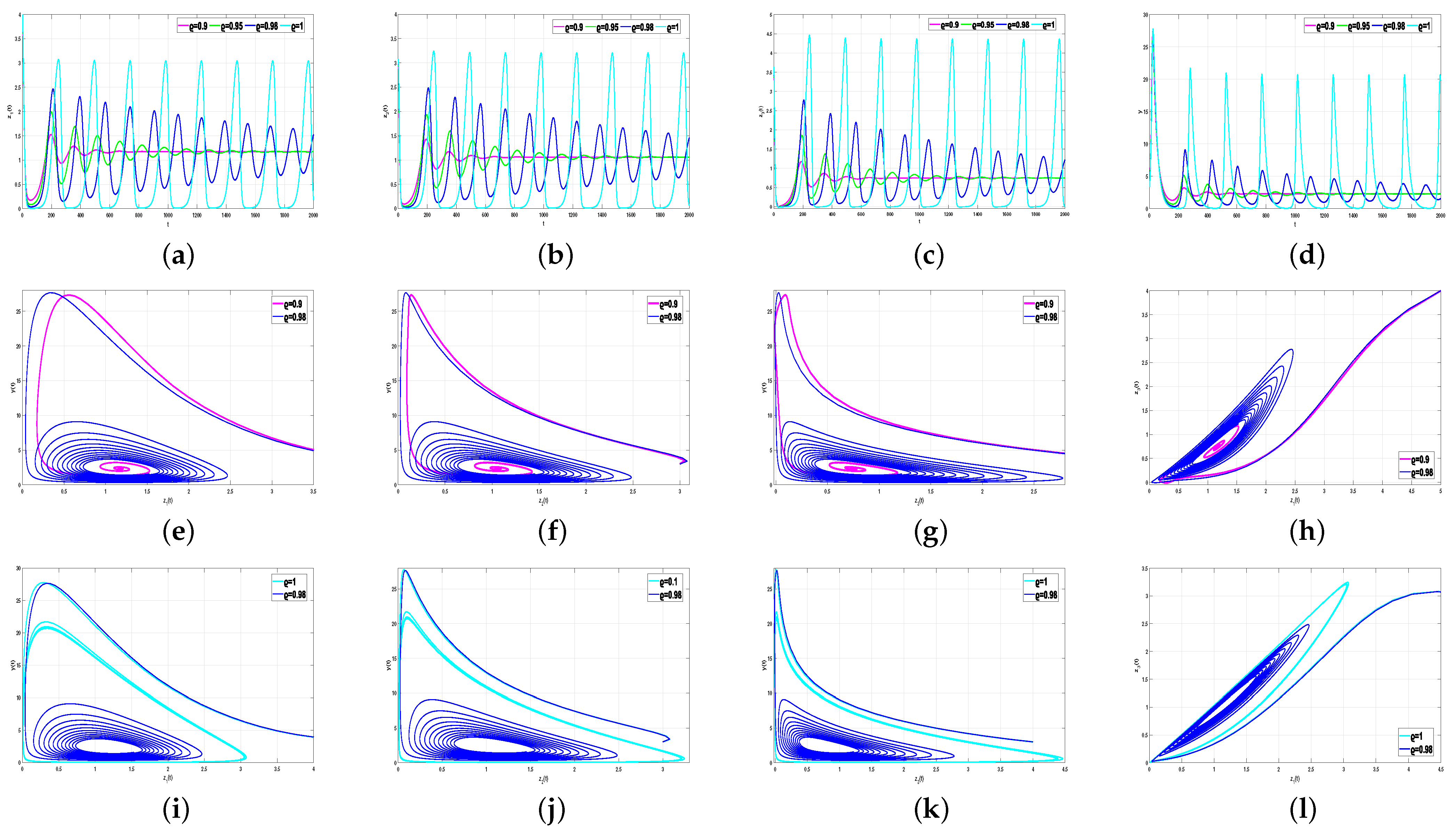
We assume $\tau =0$. Figure 1 shows the $z_1\left(t\right),z_2\left(t\right),z_3\left(t\right)$, and $y\left(t\right)$ under four different sets of $\varrho$ convergence to $E_4$ time series. It is easy to observe that the convergence rate is affected by different fractional order values. With the gradual increase in $\varrho$, the oscillation behavior becomes more and more serious.

Remark 2.

The fractional order reflects the memory and historical dependencies of the system. The greater the order, the stronger the memory and dependence of the system on the previous state. This long-term memory effect makes the dynamic behavior of the system more complex and sensitive and easily leads to large fluctuations.

Example 2.

The effect of time delays on system stability and Hopf bifurcation.

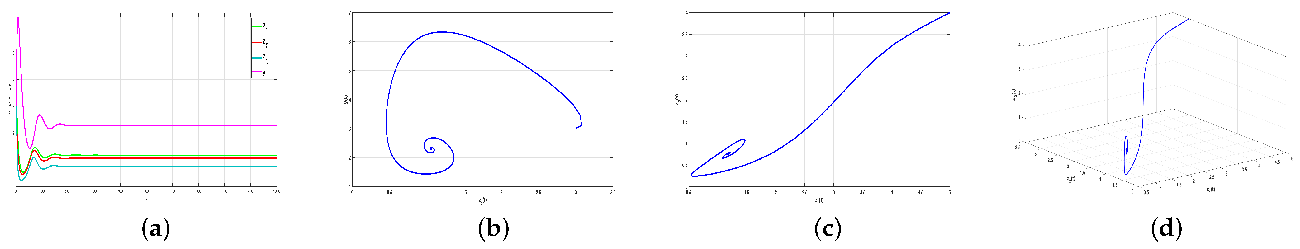
First, we set $\varrho =0.98$ and verify that $\Delta >0(i=1,2,3,4)$ when $\tau =0$. Therefore, the coexistence equilibrium point $E_4$ of system (5) reaches a stable state without delay, as shown in Figure 2. Subsequently, using Equations (34) and (35), we obtain ${\tau }_0=0.853$. The calculation confirms that the condition H(2) is satisfied, implying that Hopf bifurcation occurs when system (5) meets the crossing condition at ${\tau }_0$. When $\tau =0.75<{\tau }_0$ is selected, system (5) is locally asymptotically stable at $E_4$. The numerical results are shown in Figure 3. Conversely, when $\tau =1.1>{\tau }_0$ is selected, system (5) becomes unstable at $E_4$. The numerical results are shown in Figure 4. The correctness of Theorem 7 is verified based on the stability changes shown in Figure 3 and Figure 4.

Next, we set $\tau =1.1$, change the value of $\varrho$, and examine the time series and phase diagram of system (5) at $E_4$. We set $\varrho =0.9,0.95,0.98,1$. The numerical results are shown in Figure 5. From the above calculation, ${\tau }_0=0.853$ when $\varrho =0.98$; thus, system (5) exhibits an unstable state at $E_4$ when $\tau =1.1$, as shown in Figure 4. However, in Figure 5, when $\varrho =0.85,0.9,$ system (5) is stable at $E_4$, indicating that the bifurcation critical value of the system ${\tau }_0>0.853$ at this time, while system (5) is extremely unstable at $E_4$ when $\varrho =1$. This implies that the bifurcation point ${\tau }_0$ of an integer order system must be less than $0.853$. These results reflect the relationship between $\varrho$ and ${\tau }_0$; that is, the larger the value of $\varrho$, the smaller that of ${\tau }_0$.

7. Conclusions

A fractional-order time-delay predation model with a three-stage structure and cannibalism in the prey was established. For the first time, the local stability of each equilibrium point in a system without a time delay was analyzed by considering a case in which predators hunt both adults and old prey. The explicit conditions for the Hopf bifurcation were derived by considering the digestion delay of the predator as a bifurcation parameter. The theoretical results are verified through numerical simulations. In addition, in the numerical example, different fractional-order orders $\varrho$ were selected for numerical simulation. The results demonstrate that the stable states generated by different fractional orders $\varrho$ have different stability rates, highlighting the complexity of the fractional-order system dynamics. Finally, the advantages of fractional differential equations, which have a larger stable region than integer-order systems, were emphasized. Because the time delay of the fractional-order system can cause Hopf bifurcation, setting an effective controller to reduce the bifurcation will be the focus of our future research.

In addition, the power-law predator–prey models are another specific type of mathematical models used to describe the interaction between predators and prey in an ecosystem. One of the main advantages of using power-law predator–prey models is their ability to capture complex and non-linear behaviors that may not be accounted for in simpler linear models. They can potentially provide more accurate predictions and a deeper understanding of ecological systems [43]. Therefore, there will be interesting future work, such as investigating the dynamics of the fractional-order power-law predator–prey models.