Method for Measuring the Fractional Derivative of a Two-Dimensional Magnetic Field Based on Taylor–Riemann Series

Abstract

In magnetic data processing, a fractional derivative can enhance details without excessively amplifying high-frequency noise. To obtain a fractional derivative numerically, a large number of survey points are required. This article demonstrates how a few survey points can be used to obtain the fractional derivative of a two-dimensional magnetic field through the application of Taylor–Riemann series. First, we derive the measurement method for the fractional gradient. This method is achieved by measuring the magnetic field at several survey points on a circle, then constructing analytical functions and finally calculating the fractional derivative. Next, an experiment is designed and simulated to demonstrate the impact of the fractional derivative start point and the ability to suppress Gaussian noise. Finally, the experiment is performed, which verifies the feasibility of the proposed method in a two-dimensional magnetic field.

1. Introduction

The concept of fractional calculus appears almost at the same time as integer-order calculus [1]. There are many definitions of fractional calculus, some of which are defined for specific applications. Some of them are the Riemann–Liouville (RL) fractional calculus [2], the Grunwald–Letnikov (GL) fractional calculus [3], the Caputo fractional calculus [4], the Atangana–Baleanu (AB) fractional calculus [5,6], the Riesz fractional calculus [7], the Weyl fractional calculus [8], etc. The most general definitions are the RL and GL definitions which are independent of specific applications. They are obtained by generalizing the order of integer-order derivative to an arbitrary real number [9]. In the field of complex analysis, the Cauchy integral formula can also be extended to the fractional order [10].

Fractional order calculus has been widely applied to the modeling and analysis of magnetic phenomena. Aykuta and Beyhana research the effect of fractional analysis on magnetic curves and investigate the trajectories of the magnetic fields [11]. Fractional calculus has been applied to the scalar Helmholtz equation [12]. It has also been used to extend Maxwell’s equations [13]. Although fractional calculus has been widely used, there is currently no universal and concise explanation for fractional calculus. Podlubny proposes a geometric and physical explanation for RL calculus [14]. He interprets the RL integration as the displacement of an object observed in a distorted coordinate system, which can be illustrated as the projection of a fence on two walls. Bai and Xue [15] interpret the 1/2-order RL integral as a curvilinear integral of a specific function along a semicircle. However, both explanations have limitations. Podlubny’s interpretation specifies the motion function of the observer. Bai and Xue’s interpretation specifies the integral order to be 1/2, the integral path to be a semicircle, and the integrand to be a specific function. These non-universal explanations limit their applications.

Since there is no general physical meaning for fractional calculus, in the field of magnetic exploration, fractional calculus is currently used primarily for data processing without considering their physical meanings. These studies primarily utilize the transitional properties of fractional derivatives by adjusting the derivative order to enhance details without excessively amplifying high-frequency noise. Since the 1930s, the derivative of the magnetic data has been used to enhance the details of magnetic anomaly and to suppress slowly changing background fields [16]. This operation behaves like a high-pass filter in the frequency domain [17]. It is susceptible to noise. As the order of the derivative increases, the noise is amplified, and the signal is submerged. The derivative operation is used only to enhance details and has no other physical meaning. From a mathematical perspective, there is no reason to limit the derivative order to integers.

Gunn [18] presents a novel algorithm for enhancing the visual representation of airborne geophysical data. The author uses the fractional derivative to address the issue of noise but does not mention the methodology for evaluating the value of the fractional derivative. Cooper and Cowan [19] use a numerical algorithm [20] to calculate the fractional gradients of magnetic data, thereby achieving a balance between noise and resolution. Furthermore, the fractional derivative is applied to the sunshading operation [21], which is a high-pass filter, to reduce the impact of noise. The shallow-layer separation filter is capable of separating the regional and residual magnetic fields, which is important for magnetic interpretation [22]. Cooper and Cowan extend the vertical derivative to the fractional order, providing a flexible approach to shallow-layer separation filtering. Arisoy [23] uses the fractional derivative to enhance and detect the edge of magnetic data, which is achieved by adjusting the order of the fractional derivative. Arisoy transforms the calculation of the fractional derivative into the frequency domain to reduce the requirements of memory size caused by the nonlocality property of the fractional derivate.

Due to the complexity of the definition of fractional calculus, a numerical method is applied to field data in the above applications to obtain fractional derivatives. The numerical method requires a large number of samples to meet accuracy requirements. In contrast to fractional calculus, the physical interpretation of an integer-order derivative is clear. Therefore, the magnetic gradient can be measured directly. This is accomplished by measuring the field at two points and, then, dividing the magnetic difference by the distance between the two points [24]. The first widely recognized instrument used in aeromagnetic measurement is the low-temperature superconducting magnetic gradiometer developed by the Jena Institute for Advanced Technology in Germany in 1997. The experiments were conducted in South Africa, and they obtained the full tensor gradient data graph [25]. In 2010, National Laboratory of Singapore developed a differential tensor instrument with a cross-shaped structure for underwater magnetic measurement [26]. An Italian team developed a differential tensor instrument with a triangular pyramid structure [27]. University of Defense Technology and Jilin University also developed a differential tensor instrument with a cross-shaped structure [28,29].

Can a fractional gradient of the magnetic field be obtained directly from fewer survey points? Tilbrook established the relationship between the magnetic field and its derivatives through the Taylor series of the magnetic field. The orders of the field derivatives correspond to the index of the series terms. When flux gate sensor rotates about an external axis, its output voltage is modulated by the magnetic field and its derivatives of different orders. Since the terms in the Taylor series also correspond to the harmonics of the voltage, the field derivatives can be further obtained [30]. Inspired by his work, the Taylor–Riemann (TR) series is introduced [31]. The terms of the TR series include the fractional derivative factor. We truncate the TR series to approximate the original function. Then, we measure the magnetic field at several points and take them as the original functions to be expanded by the unknown TR series. Take these series as equations and the unknowns as the factors of these TR series. Finally, the fractional derivatives of the field are obtained by solving these equations. In this way, we can obtain the fractional derivative of the magnetic field with fewer survey points and make it possible to measure the fractional derivatives in real time.

2. Derivation of the Measurement Principle

2.1. Introduction to Fractional Derivative

The fractional derivative is a generalization of the integer-order derivative. There are many definitions of the fractional derivative based on different generalizations. The definitions used in this article are the GL fractional derivative, the RL fractional derivative and the Cauchy-type fractional derivative.

The GL fractional derivative comes from the limit of the difference quotient of the higher-order integer-order derivative. It is often used in numerical computations. The definition of the GL fractional derivative at $t$ is as follows:

$$\begin{array}{c}{{}_{t_0}{}^{GL}D}_t^{\alpha }f\left(t\right)=\underset{h\to 0}{\lim }\frac{1}{h^{\alpha }}{\displaystyle \sum _{j=0}^{\left[\left(t-t_0\right)/h\right]}}{\left(-1\right)}^j\left(\begin{array}{c}\alpha \\ j\end{array}\right)f\left(t-jh\right),\end{array}$$

where $t_0, t$ denote the start point and end point of the derivative, respectively. $\alpha$ denotes the order of the derivative. $h$ denotes the size of sampling grid. Function [⋅] returns the nearest integer. In this article, we take the GL derivative to obtain the numerical result of the fractional derivative of the magnetic field.

The RL fractional integral is derived from the higher-order integral. It does not involve the limit operation and is often used in analytical analysis. The RL fractional integral at $t$ is as follows:

$${{}_{t_0}{}^{RL}D}_t^{-\alpha }f\left(t\right)=\frac{1}{\mathsf{\Gamma }\left(\alpha \right)}{\int }_{t_0}^t\frac{f\left(\tau \right)\mathrm{d}\tau }{{\left(t-\tau \right)}^{1+\alpha }},$$

where $\alpha >0$. The RL fractional derivative is the integer-order derivative of the RL integral:

$${{}_{t_0}{}^{RL}D}_t^{\alpha }f\left(t\right)=\frac{1}{\mathsf{\Gamma }\left(n-\alpha \right)}\frac{{\mathrm{d}}^n}{\mathrm{d}{t}^n}{\int }_{t_0}^t\frac{f\left(\tau \right)\mathrm{d}\tau }{{\left(t-\tau \right)}^{1+\alpha -n}},$$

where $n=⌈\alpha ⌉$. The ceiling function $⌈\cdot ⌉$ returns the smallest integer which is not less than the input number. If the function $f\left(t\right)$ is $(n-1)$-times continuously differentiable in the interval $[t_0, t]$ and $f^{\left(n\right)}\left(t\right)$ is integrable in $[t_0, t]$, the GL and RL fractional derivatives of $f\left(t\right)$ are equivalent [32]. In this article, we use the RL definitions to derive the expression for the fractional derivative of the two-dimensional magnetic field.

Cauchy-type fractional calculus is a generalization of Cauchy’s integral formula. Cauchy-type fractional calculus at $w$ is as follows:

$$D_w^{\alpha }f\left(w\right)=\frac{\mathsf{\Gamma }\left(\alpha +1\right)}{2\pi \mathrm{i}}{\oint }_C\frac{f\left(t\right)\mathrm{d}\tau }{{\left(t-w\right)}^{\alpha +1}},$$

where $\alpha >0$. $t, \tau$ and $w$ are complex numbers. $C$ is the contour of integration. Unlike the previous two definitions, this equation holds in the complex plane. The TR series in this article is implemented based on the Cauchy-type fractional derivative.

In this article, we use these three types of fractional derivatives because they are direct extensions of integer-order derivatives without any other constraints. For example, compared to another widely used Caputo calculus, the GL, RL and TR definitions are continuous when their derivative orders approach integers, which shows a good transition. Furthermore, they are equivalent in this application, making it easy to convert and validate against each other. For definitions of fractional calculus such as the Caputo, Atangana-Baleanu, Riesz, Weyl etc., if their series contain the factors of fractional derivatives and hold in the complex plane, they can also be applied by a similar method described below.

2.2. Introduction to Taylor–Riemann Series

Riemann scratched down a generalized Taylor series based on fractional derivatives in 1847, but he never proved it. It was not until 1945 that Hardy proved that it is convergent in a weak sense [33]. Osler gave a proof of pointwise convergence of the series [34]. Munkhammar rewrote Osler’s proof, and we rewrite it as follows:

Theorem 1. 

Function $f\left(w\right)$ is analytic in some simply connected domain containing $a$, $b$ and $w$. Then we have

$$f\left(w\right)={\displaystyle \sum _{n=-\infty }^{\infty }}\frac{D_{a-b}^{\alpha +n}f\left(w\right)}{\Gamma \left(\alpha +n+1\right)}{\left(w-a\right)}^{\alpha +n},$$

(1)

where $a,b,w\in \mathbb{C}$, $w$ is on the circle $|w-a|=|b-a|, w\ne b$and $\alpha \in \mathbb{R}$.

We call (1) the Taylor–Riemann (TR) series. The derivative in (1) is the Cauchy-type fractional derivative:

$$D_{a-b}^{\alpha +n}f\left(w\right)=\frac{\mathsf{\Gamma }\left(\alpha +n+1\right)}{2\pi i}{\int }_{C\left(b, a^{+}\right)}\frac{f\left(w\right)}{{\left(w-a\right)}^{\alpha +n+1}}\mathrm{d}w$$

The contour $C\left(b,a^{+}\right)$ of the integration starts at $w=b$, encircles $w=a$ in the positive sense and returns to $w=b$.

The variable of the Cauchy-type derivative is the complex number $w=x+\mathrm{i} y$, which consists of two variables $x$ and $y$. But the other two definitions, the RL and the GL, are univariate. The TR series given by Munkhammar adopt the Cauchy-type fractional derivative in complex form, which has two variables. Therefore, it is possible to evaluate the fractional derivative of the two-dimensional magnetic field.

The variable $w$ keeps its form on both sides of (1), which makes it look like a univariable function. Can we apply the RL derivative to the complex function $f\left(w\right)$? We rewrite the definition given by Munkhammar:

Definition 1. 

Function $f\left(w\right)$ is analytic in some simply connected domain containing the points $w$ and $w_0$. Then we define

$$\left\{\begin{array}{l}\begin{array}{ll}{{}_{w_0}{}^{RL}D}_w^{\alpha }f\left(w\right)=\frac{1}{\Gamma \left(\alpha \right)}{\int }_{w_0}^w\frac{f\left(w\right)dt}{{\left(w-t\right)}^{1-\alpha }}& \alpha <0\\ {{}_{w_0}{}^{RL}D}_w^{\alpha }f\left(w\right)=\frac{d^m}{d{w}^m}\left[{{}_{w_0}{}^{RL}D}_w^{-\left(m-\alpha \right)}f\left(w\right)\right], m=⌈\alpha ⌉,& \alpha \ge 0\end{array}\end{array}\right.$$

with integration along the straight line connecting $w$ and $w_0$.

Then, the relationship between the Cauchy-type fractional derivative and the RL derivative is [31]:

Theorem 2. 

The function $f\left(w\right)$ is analytic in some simply connected domain containing $w_0$ and $w$. Then, the Cauchy-type fractional integral of $f\left(w\right)$ is a complex generalization of the Riemann–Liouville fractional derivative

$$D_{w-w_0}^{\alpha }f\left(w\right)={{}_{w_0}{}^{RL}D}_w^{\alpha }f\left(w\right),$$

for all $\alpha \in \mathbb{R}$, except $\alpha \in \mathbb{Z}$.

Therefore, the Cauchy-type fractional derivative can be transformed into the RL derivative by changing the contour from circle $C$ to line $L$, as shown in Figure 1. In addition, the RL derivative is equivalent to the GL derivative. In this article, the GL derivative is used to verify the result of the RL derivative.

Figure 1. Contour of Cauchy-type fractional integration.

2.3. Implementation of the Measurement Principle

The Taylor–Riemann series (1) is an infinite series. It must be truncated to a finite series to approximate the function $f\left(w\right)$. In the proof given by Munkhammar, $k$ is also the dummy index of the Fourier series coefficients. Therefore, the terms must be symmetric about $k=0$, and the number of terms $2K+1$ is always odd and $N=2K+1$. Now, truncate it to N terms about $k=0$:

$$\begin{array}{ll}f\left(w\right)=& c_0\left(w\right){{}_b{}^{\mathrm{R}\mathrm{L}}D}_a^{\alpha }f\left(w\right)\\ & +\left[c_1\left(w\right){{}_b{}^{\mathrm{R}\mathrm{L}}D}_a^{\alpha +1}f\left(w\right)+c_{-1}\left(w\right){{}_{b}D}_a^{\alpha -1}f\left(w\right)\right]\\ & +\dots \\ & +\left[c_k\left(w\right){{}_b{}^{\mathrm{R}\mathrm{L}}D}_a^{\alpha +k}f\left(w\right)+c_{-k}\left(w\right){{}_{b}D}_a^{\alpha -k}f\left(w\right)\right]\\ & +\dots \\ & +\left[c_K\left(w\right){{}_b{}^{\mathrm{R}\mathrm{L}}D}_a^{\alpha +K}f\left(w\right)+c_{-K}\left(w\right){{}_{b}D}_a^{\alpha -K}f\left(w\right)\right],\end{array}$$

where $a$, $w$ satisfy $| w-a |=|b-a |$. The coefficient $c_k\left(w\right)$ is as follows:

$$c_k\left(w\right)=\frac{{\left(w-a\right)}^{\alpha +k}}{\mathsf{\Gamma }\left(\alpha +k+1\right)}.$$

Our goal is to evaluate the fractional derivative ${{}_{b}D}_a^{\alpha }f\left(w\right)$, which is one of the unknown derivatives ${{}_{b}D}_a^{\alpha +k}f\left(w\right)$. This can be carried out by solving equations. Establish $N=2K+1$ equations as (2) by changing the position $w$ on the circle $C$:

$$\left\{\begin{array}{c}f\left(w_1\right)={\displaystyle \sum _{k=-K}^K}{c}_k\left(w_1\right){{}_{b}D}_a^{\alpha +k}f\left(w\right)\\ \cdots \\ f\left(w_n\right)={\displaystyle \sum _{k=-K}^K}{c}_k\left(w_n\right){{}_{b}D}_a^{\alpha +k}f\left(w\right)\\ \cdots \\ f\left(w_N\right)={\displaystyle \sum _{k=-K}^K}{c}_k\left(w_N\right){{}_{b}D}_a^{\alpha +k}f\left(w\right).\end{array}\right.$$

(2)

Rewrite it in matrix form:

$$\mathit{F}=\mathit{C}\mathit{D},$$

where $\mathit{F}=\left[f\left(w_n\right)\right]\in {\mathbb{C}}^N$, $\mathit{C}=\left[c_k\left(w_n\right)\right]\in {\mathbb{C}}^{N\times N}$ and $\mathit{D}=\left[{{}_{b}D}_a^{\alpha +k}f\left(w\right)\right]\in {\mathbb{C}}^N$, respectively. Fractional derivatives can be worked out by evaluating $\mathit{D}={\mathit{C}}^{-1}\mathit{F}$. It is difficult to evaluate ${\mathit{C}}^{-1}$ directly, and we decompose it into ${\mathit{C}}^{-1}={\left(\mathit{P}\mathit{Q}\mathit{R}\right)}^{-1}={\mathit{R}}^{-1}{\mathit{Q}}^{-1}{\mathit{P}}^{-1}$. Let $r=\left|b-a\right|=|w_n-a|$ and ${\theta }_n=\mathrm{A}\mathrm{r}\mathrm{g}\left(w_n-a\right)$, then:

$$\mathit{P}=\left[\begin{array}{cccc}{\left(r{e}^{\mathrm{i}{\theta }_1}\right)}^{\alpha }& & & \\ & {\left(r{e}^{\mathrm{i}{\theta }_2}\right)}^{\alpha }& & \\ & & \ddots & \\ & & & {\left(r{e}^{\mathrm{i}{\theta }_N}\right)}^{\alpha }\end{array}\right],$$

$$\mathit{Q}=\left[\begin{array}{cccc}{e}^{\mathrm{i}\left(-K\right){\theta }_1}& e^{\mathrm{i}\left(-K+1\right){\theta }_1}& \cdots & e^{\mathrm{i}K{\theta }_1}\\ e^{\mathrm{i}\left(-K\right){\theta }_2}& e^{\mathrm{i}\left(-K+1\right){\theta }_2}& \cdots & e^{\mathrm{i}K{\theta }_2}\\ ⋮& ⋮& & ⋮\\ (e^{\mathrm{i}\left(-K\right){\theta }_N}& e^{\mathrm{i}\left(-K+1\right){\theta }_N}& \cdots & e^{\mathrm{i}K{\theta }_N}\end{array}\right],$$

$$\mathit{R}=\left[\begin{array}{cccc}\frac{r^{-K}}{\mathsf{\Gamma }\left(\alpha \right)}& & & \\ & \frac{r^{-K+1}}{\mathsf{\Gamma }\left(\alpha +1\right)}& & \\ & & \ddots & \\ & & & \frac{r^K}{\mathsf{\Gamma }\left(\alpha +N-1\right)}\end{array}\right].$$

$\mathit{P}$ and $\mathit{R}$ are diagonal matrices, and it is easy to calculate their inverse. Rewrite the equation as $\mathit{D}=\left({\mathit{R}}^{-1}{\mathit{Q}}^{-1}\right)\left({\mathit{P}}^{-1}\mathit{F}\right)$. Since we only take the element ${{}_{b}D}_a^{\alpha }f\left(w\right)$ in $\mathit{D}$, the corresponding row is the central row of ${\mathit{Q}}^{-1}$. $N$ is the number of survey points on the circle $C$. Too many survey points make them close to each other, and the magnetic field measured at survey points become similar. Therefore, we usually take no more than nine survey points on the circle. With the help of software Mathematica (Version 12.1, Wolfram Research, Champaign, IL, USA, Inc.), we find that the central row of ${\mathit{Q}}^{-1}$ is $\left(\frac{1}{N}, \frac{1}{N}, \dots , \frac{1}{N}\right)\in {\mathbb{R}}^N$ for $N=3, 5, 7, 9$. The others are $1/\mathsf{\Gamma }\left(\alpha +\frac{N-1}{2}\right)$ in ${\mathit{R}}^{-1}$ and the diagonal of ${\mathit{P}}^{-1}$. Therefore,

$${{}_{b}D}_a^{\alpha }f\left(w\right)=\frac{\mathsf{\Gamma }\left(\alpha +\frac{N-1}{2}\right)}{N{r}^{\alpha }}{\displaystyle \sum _{n=1}^N}{e}^{-\mathrm{i}\alpha {\theta }_n}f\left(w_n\right).$$

(3)

After the above preparation, we next apply the above process to magnetic field components. The magnetic field components $B_x\left(w\right)$ and $B_y\left(w\right)$ of the two-dimensional magnetic field are used to construct the function $f\left(w\right)$:

$$f\left(w\right)=B_y\left(w\right)+\mathrm{i}{B}_x\left(w\right)$$

(4)

where $x$ is the real axis of complex plane, and $y$ is the imaginary axis. Equation (4) must be analytic in the complex plane $Oxy$. That is, it must satisfy Cauchy–Riemann conditions:

$$\frac{\partial B_y}{\partial x}=\frac{\partial B_x}{\partial y},$$

(5)

$$\frac{\partial B_y}{\partial y}=-\frac{\partial B_x}{\partial x}.$$

(6)

It is known that the magnetic field is a passive field, and its divergence in three-dimensional space is 0, which can be expressed as follows:

$$\frac{\partial B_x}{\partial x}+\frac{\partial B_y}{\partial y}+\frac{\partial B_z}{\partial z}=0.$$

(7)

In area without current distribution, the magnetic field is irrotational:

$$\left\{\begin{array}{c}\frac{\partial B_x}{\partial y}-\frac{\partial B_y}{\partial x}=0\\ \frac{\partial B_x}{\partial z}-\frac{\partial B_z}{\partial x}=0\\ \frac{\partial B_y}{\partial z}-\frac{\partial B_z}{\partial y}=0.\end{array}\right.$$

(8)

The irrotational property (8) makes $f\left(w\right)$ satisfy (5). But for (6), it can only be satisfied when $\frac{\partial B_z}{\partial z}=0$ in (7), which means that the magnetic field component perpendicular to the complex plane remains unchanged in its direction. Therefore, this method is available for two-dimensional magnetic field.

Solution ${{}_{b}D}_a^{\alpha }f\left(w\right)$ is also a complex number. According to the linear property of fractional derivative, it can be written as follows:

$${{}_{b}D}_a^{\alpha }f\left(w\right)={{}_{b}D}_a^{\alpha }{B}_y\left(w\right)+\mathrm{i}{{}_{b}D}_a^{\alpha }{B}_x\left(w\right).$$

(9)

To determine the value of $c_k$ in (2), it is necessary to determine the center $a$ and the radius $|a-b|$ of the circle $C$, as well as the position $w_n$ of the survey points on the circle $C$. For other variables, $k$ is the dummy index, and $\alpha$ is the derivative order.

The principle of measuring two-dimensional magnetic anomalies using the TR series has been derived above. Next, an example is designed to simulate the measurement process.

3. TR Method Simulation

3.1. Simulation Setup

In this example, current-carrying wires are used to generate a two-dimensional magnetic field. The simulation setup is shown in Figure 2.

Figure 2. Simulation setup.

A pair of long wires with the length of $l_z$ is perpendicular to the complex plane. Their coordinates in the complex plane are $s_1=\frac{\mathrm{i}}{2} \mathrm{m}$ and $s_2=-\frac{\mathrm{i}}{2} \mathrm{m}$. The complex plane is located at the center of long wires. The wires carry a current of 14.4 A in opposite directions. Take the circle $C:\left|w-a\right|=\left|b-a\right|$, $a=0.25 \mathrm{m}$ in the complex plane. During actual measurement, the magnetic field is unknown, so we set survey points $w_n(n<N,N=5)$ uniformly distributed on circle $C$. We evaluate the fractional derivative at $a=0.25 \mathrm{m}$ by the magnetic components $B_x$, $B_y$ measured at $w_n$ on the circle. Next, we have to determine the length $l_z$ to make it similar enough to a two-dimensional field.

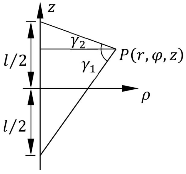
The cylindrical coordinate system is established. One of the long wires is the rotation axis $z$, and the center of the wire is the origin, as shown in Figure 3. The complex plane is perpendicular to the $z$-axis and passes through the point $P\left(\rho ,\phi ,z\right)$. $\phi$ is the rotation angle in the cylindrical coordinate system.

Figure 3. Evaluate the magnetic field of the finite line current.

When $\phi =0$ and ${\gamma }_1=-{\gamma }_2=\gamma$, the magnetic field at point $P\left(\rho ,\phi ,z\right)$ is given by the following:

$$\mathit{B}\left(\rho ,z\right)=\frac{{\mu }_{0}I}{2\pi \rho }\sin \gamma {\mathit{e}}_{\phi }.$$

(10)

Since there is no component in z direction, any straight line can generate a two-dimensional field. The factor $\sin \gamma$ only affects the field strength. When $\gamma \to \frac{\pi }{2}$,$\sin \gamma \to 1$. The length of the wire tends to be infinity with respect to $\rho$, and the field can be regarded as a two-dimensional field. In practice, the length can be increased to approximate the infinite case.

In addition, the impact of the short sides with the length of $l_y$ must be considered. It can be seen from (10) that the long sides with the length of $l_z$ do not generate the magnetic field component $B_z$. Short sides and long sides form a current loop, and the short sides produce the magnetic field component $B_x$, and the gradient $\frac{\partial B_x}{\partial x}$ (component $B_z$ disappears in the complex plane because of the symmetric position of the short sides around the complex plane and the inverse direction of the current). They are added to the magnetic field and the magnetic derivative of two long sides, which can make the magnetic field away from $B_x$ of the infinitely long wire and violate the constraint $\frac{\partial B_x}{\partial x}+\frac{\partial B_y}{\partial y}=0$. Therefore, the short sides must be away from the complex plane, which can also be achieved by increasing $l_z$.

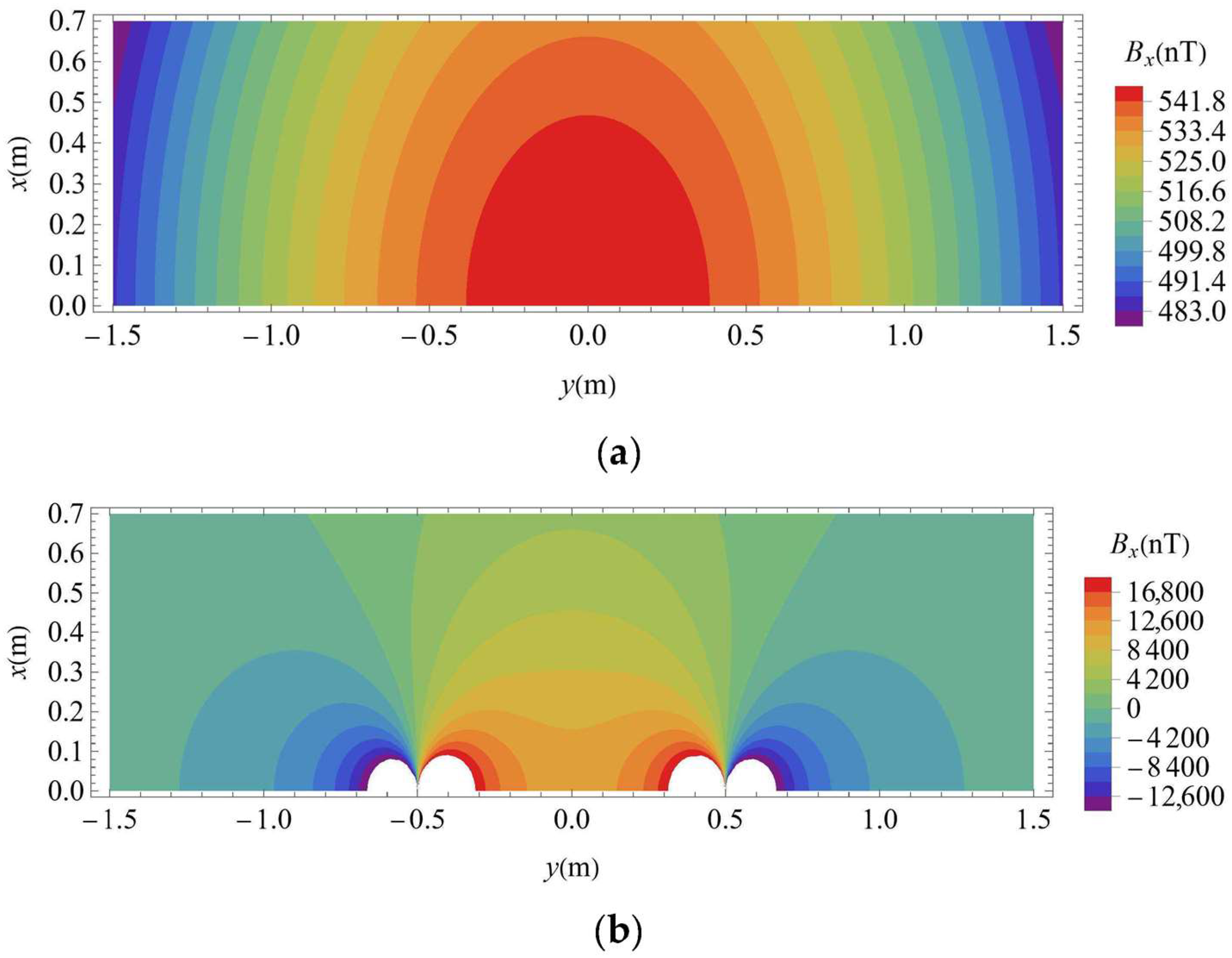
When $l_z=10.5 \mathrm{m}$, in the complex plane, the contours of $B_x$ of short sides and long sides are shown in Figure 4. The range of Figure 4 covers the measurement area.

Figure 4. (a) $B_x$ of short sides; (b) $B_x$ of long sides.

For the vertex at 0.7 + 1.5 i that is farthest from the left line source, $\sin \gamma$ = 0.9273. It means that the strength of the magnetic field generated by the finite long wire is at least 92.73% of that of an infinitely long wire in this region. We consider it the field of the infinitely long wire. The overall $B_x$ of short sides is in the range of 479 nT~546 nT, while that of the long sides is thousands of nanotesla in most of the given range. We also plot the contours of $\frac{\partial B_x}{\partial x}$ of the short sides and long sides separately in Figure 5.

Figure 5. (a) $B_{xx}$ of the short sides; (b) $B_{xx}$ of the long sides.

The situation is similar to the previous one. $\frac{\partial B_x}{\partial x}$ of the long sides is quite larger than that of the short sides. Therefore, the short sides hardly affect $B_x$ and $\frac{\partial B_x}{\partial x}$ generated by the long sides.

3.2. Single Point Simulation

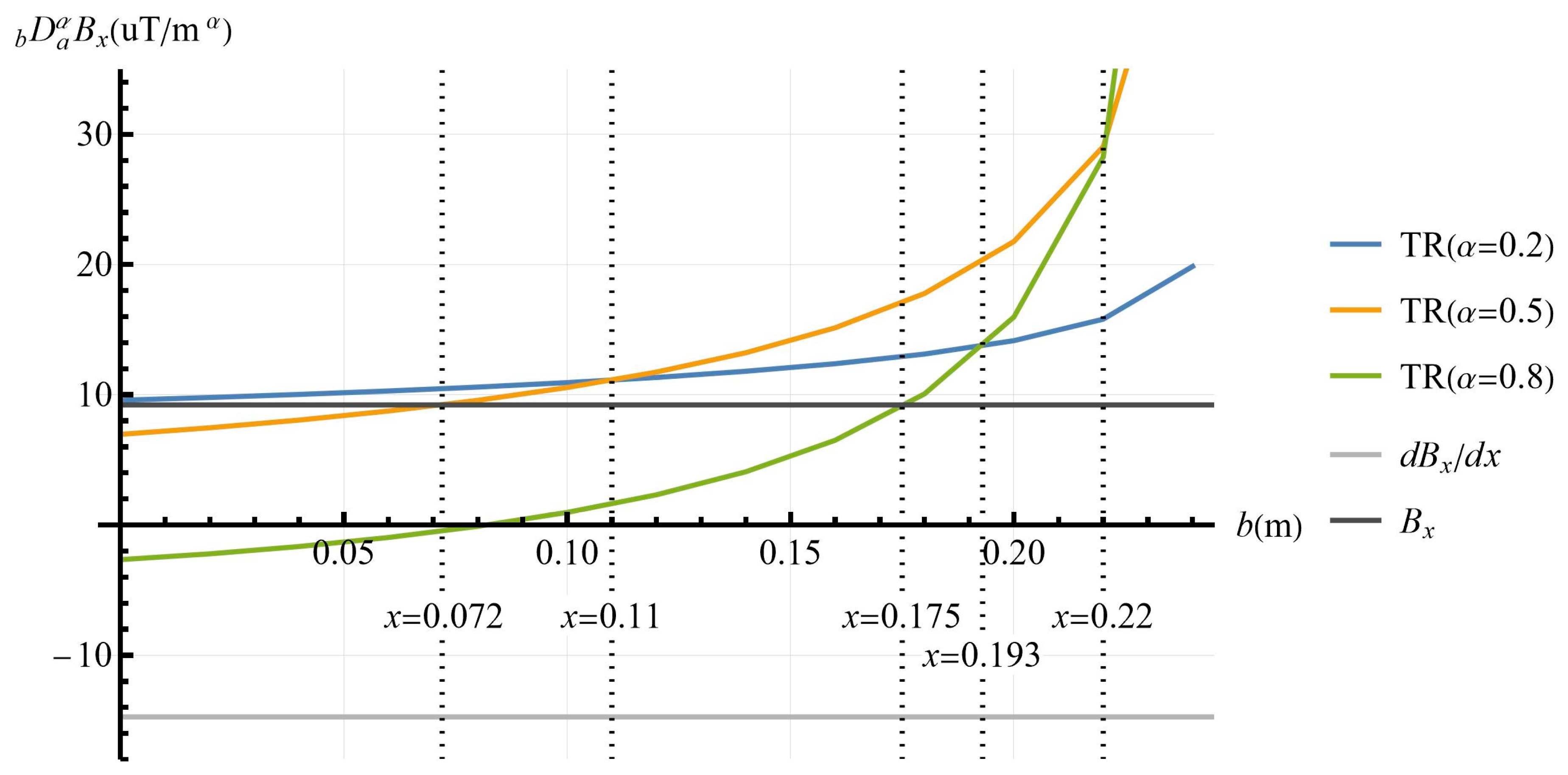
After determining the magnetic field, we perform a single point simulation to obtain the fractional derivative at $w=a$. First, we generate the magnetic field component $B_x$, $B_y$ at the survey points $w_n$ and construct $f\left(w_n\right)$ according to (4). Then, we substitute all parameters into (3) and evaluate it. Finally, we separate ${{}_{b}D}_a^{\alpha }{B}_y$ and ${{}_{b}D}_a^{\alpha }{B}_x$ from ${{}_{b}D}_a^{\alpha }f\left(w\right)$ according to (9). Since the real part ${{}_{b}D}_a^{\alpha }{B}_y$ is always 0 at $w=a$, we consider only ${{}_{b}D}_a^{\alpha }{B}_x$. Figure 6 shows ${{}_{b}D}_a^{\alpha }{B}_x$ under different derivative orders $\alpha$ and the start point $b$ of the fractional derivative.

Figure 6. ${{}_{b}D}_a^{\alpha }{B}_x$ under various derivative order $\alpha$ and start point $b$.

The curves of ${{}_{b}D}_a^{\alpha }{B}_x$ with different $\alpha$ intersect many times when the start point $b$ approaches the point $a=0.25 \mathrm{m}$. We divide these curves into several segments at the intersections and sort $\alpha$ by the value of ${{}_{b}D}_a^{\alpha }{B}_x$ in descending order in each segment. When $b\in \left[0, 0.072\right) \mathrm{m}$, the order is 0.2, 0, 0.5, 0.8, 1. Note that ${{}_{b}D}_a^0{B}_x=B_x$ and ${{}_{b}D}_a^1{B}_x=\frac{\partial B_x}{\partial x}$. When $b \in \left[0.072, 0.10\right) \mathrm{m}$, the order is 0.2, 0.5, 0, 0.8, 1. We can see that the order changes. The orders in other segments are also different. It shows that $b$ affects the peak value of ${{}_{b}D}_a^{\alpha }{B}_x$. The fractional derivative is a transition between integer-order derivatives, and the value of ${{}_{b}D}_a^{\alpha }{B}_x$ should monotonically change as $\alpha$ increases from 0 to 1. Additionally, the closer $b$ is to $a$, the larger the value of ${{}_{b}D}_a^{\alpha }{B}_x$, which is unstable. Therefore, $b$ must be set to keep the derivative interval $\left|b-a\right|$ wide enough as the first segment shown in Figure 6.

According to the definition of the GL derivative, we can also measure the GL derivatives on the interval from the start point $b$ to the end point $a$ by sampling magnetic fields on the interval. It is another method to calculate the fractional derivative of the magnetic field. Because the GL and RL definitions are equivalent, we can verify the TR method by the GL method. We take $N_s$ = 10, 30, 100 survey points on the survey line from $b$ to $a$, and their results are shown in Figure 7.

Figure 7. ${{}_{b}D}_a^{\alpha }{B}_x$ obtained by the GL and TR methods. Number of samples in the GL method: (a) $N_s$ = 10; (b) $N_s$ = 30; (c) $N_s$ = 100.

Open markers denote ${{}_{b}D}_a^{\alpha }{B}_x$ obtained by the numerical method according to the GL definition. When there is no noise, regardless of the number $N_s$ of survey points in the GL method, the open markers almost overlap the corresponding line obtained by the TR series. Therefore, the value of ${{}_{b}D}_a^{\alpha }{B}_x$ obtained by the TR series is reliable.

3.3. Survey Line Simulation

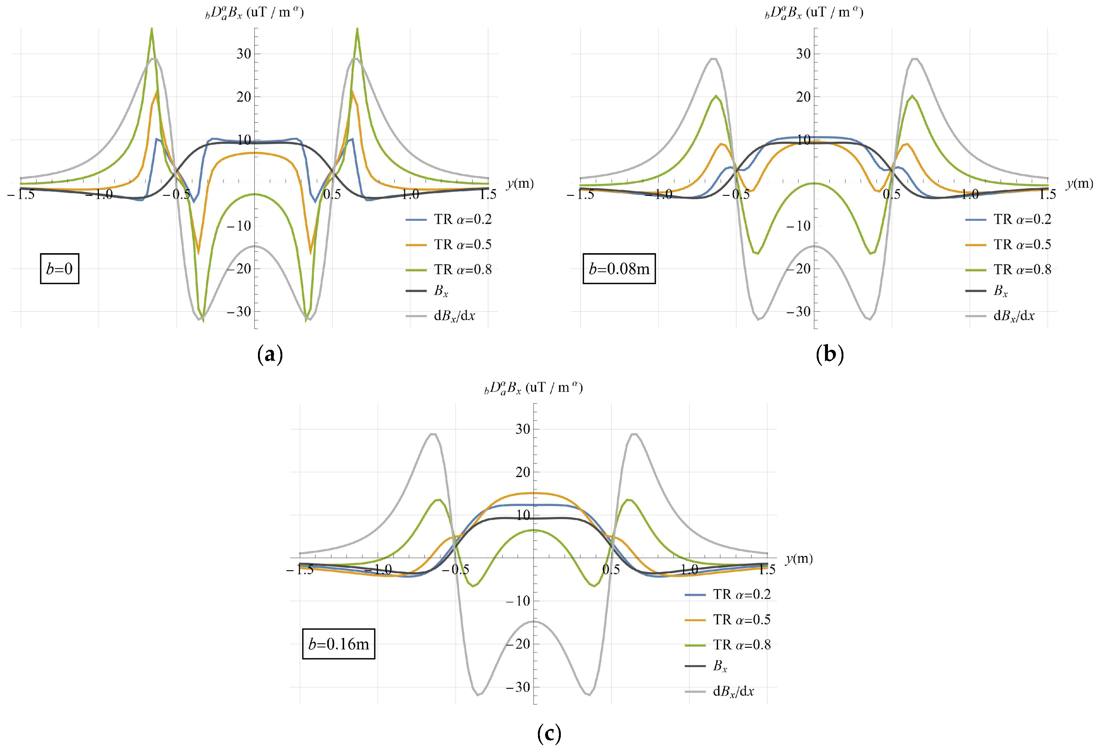
We perform a simulation on a survey line whose equation is $x=0.25 \mathrm{m}$. We also take the start point $b$ into account to show its effect. ${{}_{b}D}_a^{\alpha }{B}_x$ on the survey line is shown in Figure 8.

Figure 8. ${{}_{b}D}_a^{\alpha }{B}_x$ on the survey line when: (a) $b=0$; (b) $b=0.08 \mathrm{m}$; (c) $b=0.16 \mathrm{m}$.

In terms of the properties of the fractional derivative itself, each subplot shows the same trends that the curve of $B_x$ transforms to $\frac{\partial B_x}{\partial x}$ as the derivative order $\alpha$ increase. When $b$ = 0 and $\alpha$ = 0.5, the curve forms a flat top near the center, which is similar to the curve of $B_x$. There are two peaks around the center, which is the characteristic of $\frac{\partial B_x}{\partial x}$. As $\alpha$ decreases to $\alpha$ = 0.2, the flat top rises, and the peaks fall. This means that the partition of $B_x$ increases, and the partition of $\frac{d{B}_x}{dx}$ decreases. And it is reversed as $\alpha$ increases to $\alpha$ = 0.8. This shows that the fractional derivative has both the properties of $B_x$ and $\frac{\partial B_x}{\partial x}$. But as the start point $b$ increases and gets closer to the end point $a$, the curves get closer to each other. For example, when $b$ = 0.16 m in (c), the curves of $\alpha$ = 0.5 and 0.2 are almost the same. Therefore, the start point $b$ must not be too close to the end point $a$.

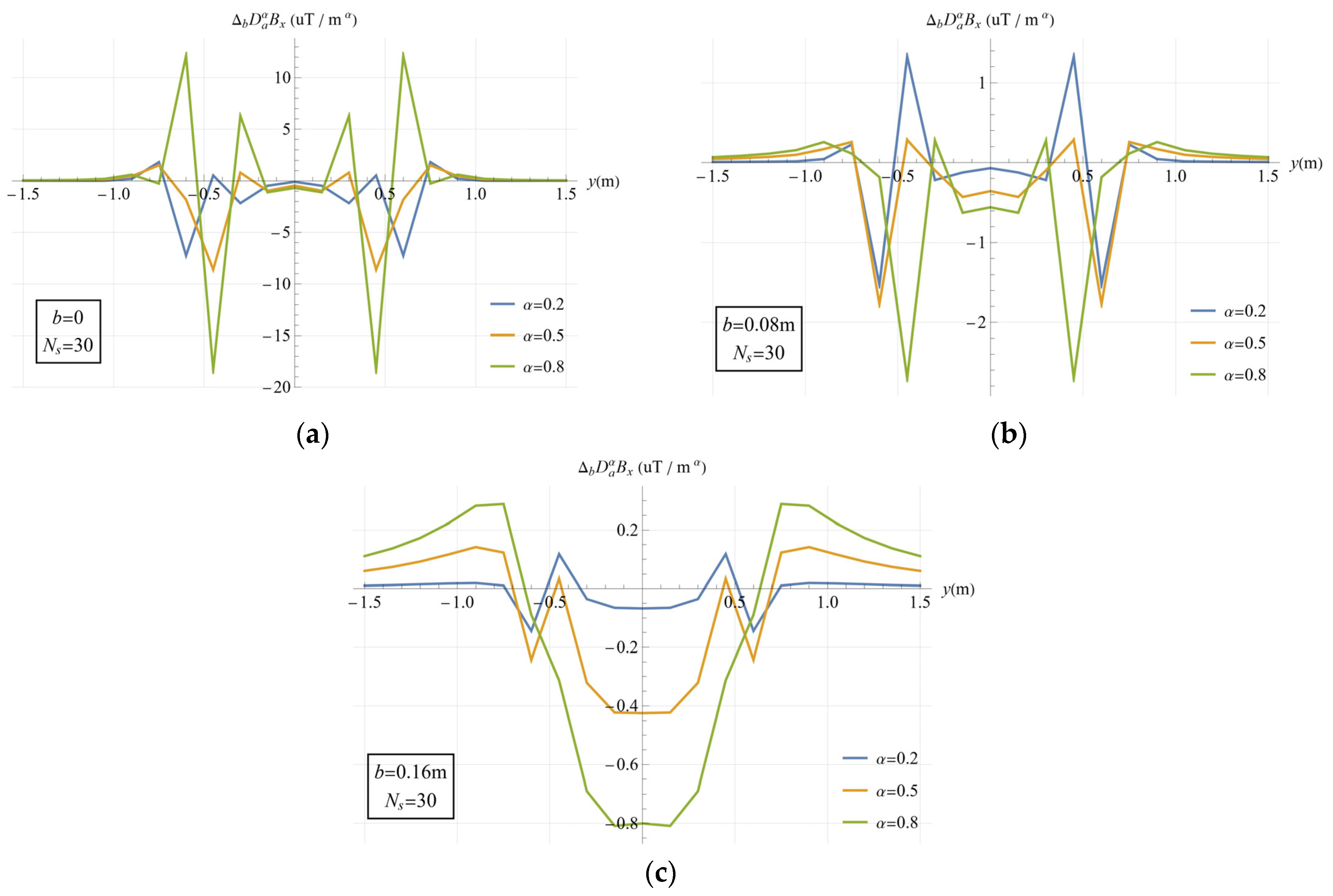
Considering there are many curves in Figure 8, to clearly compare the TR and GL methods, we just plot the difference $\mathsf{\Delta }{{}_{b}D}_a^{\alpha }{B}_x$ between them in Figure 9. Because the number $N_s$ of survey points has little effect on the result when there is no noise, we just take $N_s=30$.

Figure 9. Difference $\mathsf{\Delta }{{}_{b}D}_a^{\alpha }{B}_x$ between the TR and GL methods. (a) $b$ = 0; (b) $b$ = 0.08 m; (c) $b$ = 0.16 m.

When $b$ = 0 as shown in (a), the GL and TR derivatives are inconsistent near $y=\pm$0.5 where the line current is located. This is because circle $C$ is too large, and the distribution of survey points on circle $C$ is not dense enough to capture the drastic change in $B_x$. As $b$ increases, the circle $C$ becomes smaller, and the survey points become closer together. This allows sensors to capture more detail. For example, when $b$ = 0.08 m and $b$ = 0.16 m in (b) and (c), respectively, compared to $b$ = 0, the differences between the TR method and the GL method are smaller.

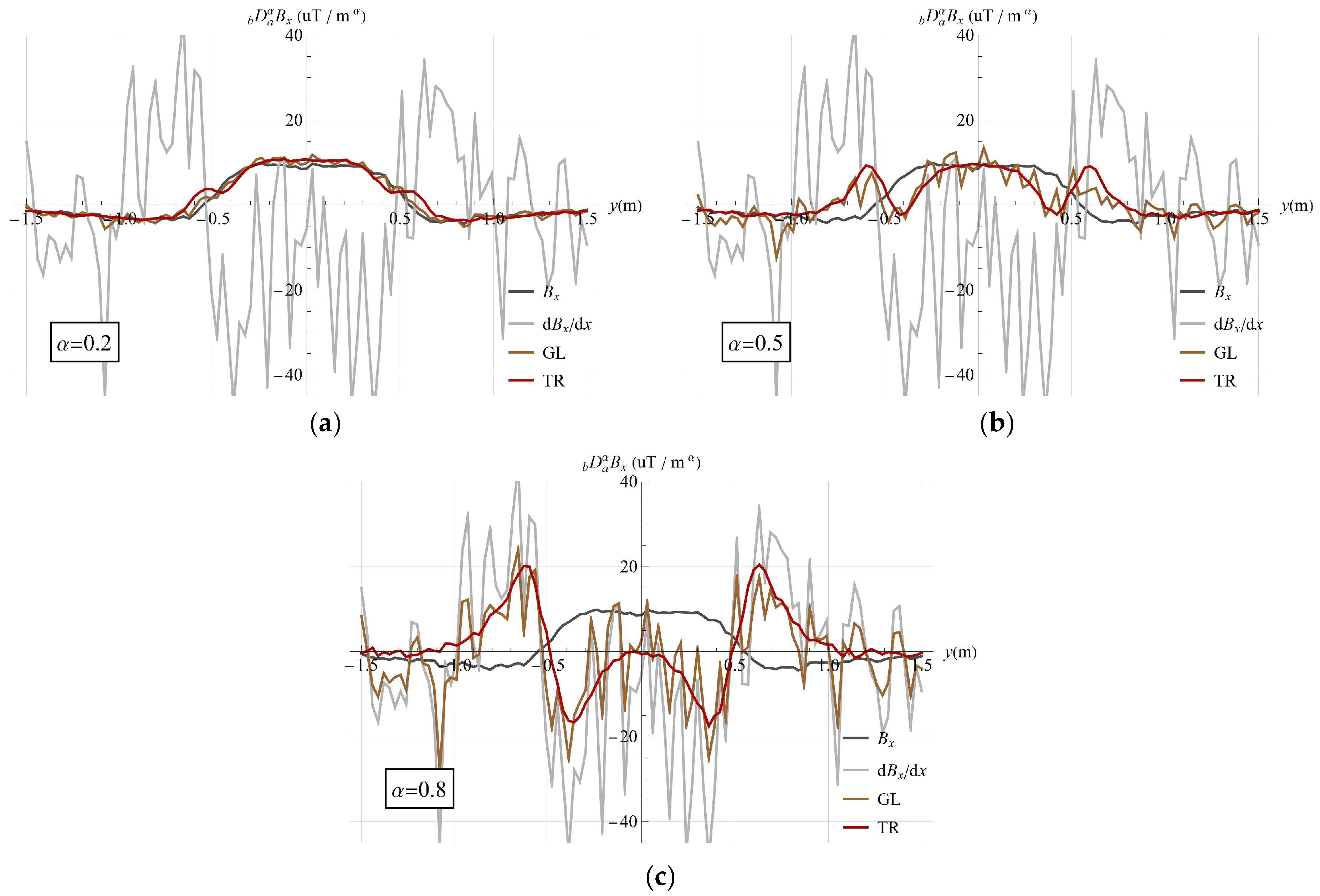
Next, we add Gaussian noise with a standard deviation ${\sigma }_x$ of 500 nT to the magnetic field component $B_x, B_y$ and simulate the measurement when $b$ = 0.08 m and $N_s$ = 5 to study the impact of the noise. The results are shown in Figure 10.

Figure 10. ${{}_{b}D}_a^{\alpha }{B}_x\left(x\right)$ on the survey line with Gaussian noise when the derivative order $\alpha$ in the TR and GL methods is: (a) $\alpha$ = 0.2; (b) $\alpha$ = 0.5; (c) $\alpha$ = 0.8.

Focusing on the curves of the GL method and $\frac{\partial B_x}{\partial x}$, we find that the curves of the GL method are proportional reductions of $\frac{\partial B_x}{\partial x}$. Then, considering the curves of the TR method, the curves of the TR method are smoother than those of the GL method at the same derivative order, and their shapes are not similar to $\frac{\partial B_x}{\partial x}$ at all.

The survey points of the GL method are on the straight line from the start point $b$ to the end point $a$, which is different from the TR method. The number $N_s$ of the survey points in the GL method can also affect the result when there is noise in the magnetic field. In order to show this, we also plot ${{}_{b}D}_a^{\alpha }{B}_x\left(x\right)$ obtained by the GL method with a different number $N_s$ of survey points. The results are shown in Figure 11.

Figure 11. ${{}_{b}D}_a^{\alpha }{B}_x\left(x\right)$ of the GL and RL method. The numbers $N_s$ of survey points are the same in each row. The derivative orders $\alpha$ are the same in each column.

We can see that with the increase in the derivative order $\alpha$ in each row, the amplitudes of the GL method increase rapidly, while the results of the TR method are still stable. In each column, as the number $N_s$ of survey points in the GL method increases, the results of the GL method are increasingly affected by noise.

To explain this, we take the values of $f\left(w_n\right)$ as the complex random variable $X_n$ and the values of ${{}_{b}D}_a^{\alpha }f\left(w\right)$ as the complex random variable $Y_{TR}$ [35]. Then, we denote the variance of $X_n$ as $\begin{array}{c}D\left(X_n\right)={\sigma }^2\end{array}$. Note that ${\sigma }^2=2{\sigma }_x^2$ because $f\left(w_n\right)=B_y+\mathrm{i}{B}_x$. From (3) we can see that ${{}_{b}D}_a^{\alpha }f\left(w\right)$ is linear function of $f\left(w_n\right)$. According to the properties of variance, $Y_{TR}$ can be expressed as follows:

$$\begin{array}{c}D\left(Y_{TR}\right)={\left[\frac{\mathsf{\Gamma }\left(\alpha + \frac{N-1}{2}\right)}{N{r}^{\alpha }}\right]}^2{\displaystyle \sum _{n=1}^N}{\left|e^{-\mathrm{i}\alpha {\theta }_n}\right|}^2{\sigma }^2\\ =\frac{\mathsf{\Gamma }{\left(\alpha + \frac{N-1}{2}\right)}^2}{r^{2\alpha }}\frac{2}{N}{\sigma }_x^2.\end{array}$$

(11)

According to the definition of the GL fractional derivative, ${{}_b{}^{GL}D}_a^{\alpha }{B}_x$ is also a linear combination of $B_{x,j}$ measured on the survey line from $b$ to $a$, which can be approximated as follows:

$${{}_b{}^{GL}D}_a^{\alpha }{B}_x\approx \frac{1}{h^{\alpha }}{\displaystyle \sum _{j=0}^J}{\left(-1\right)}^j\left(\begin{array}{c}\alpha \\ j\end{array}\right)B_{x,J-j},$$

where $J=\left[\left(t-t_0\right)/h\right]$, $\left(\begin{array}{c}\alpha \\ j\end{array}\right)=\frac{\mathsf{\Gamma }\left(\alpha +1\right)}{\mathsf{\Gamma }\left(j+1\right)\mathsf{\Gamma }\left(\alpha -j+1\right)}$. Let the value of ${{}_b{}^{GL}D}_a^{\alpha }{B}_x$ be the random variable $Y_{GL}$ and the value of $B_{x,j}$ be the random variable $X_j$. The variance of $X_j$ is $D\left(X_j\right)={\sigma }_x^2$. $D\left(Y_{GL}\right)$ can be evaluated by the following:

$$D\left(Y_{GL}\right)\approx \frac{1}{h^{2\alpha }}{\displaystyle \sum _{j=0}^J}{\left(\begin{array}{c}\alpha \\ j\end{array}\right)}^2{\sigma }_x^2.$$

(12)

The magnetic gradient $\frac{\partial B_x}{\partial x}$ can be approximated by the difference quotient of $B_{x, 1}$ and $B_{x,2}$ on adjacent survey points. That is,

$$\frac{\mathrm{d}{B}_x}{\mathrm{d}x}\approx \frac{B_{x,1}-B_{x,2}}{h}.$$

Therefore, the variance of $\frac{\partial B_x}{\partial x}$ can be expressed as follows:

$$\begin{array}{c}D\left(Y\right)\approx D\left[\frac{X_1-X_2}{h}\right]\\ =\frac{2}{h^2}{\sigma }_x^2.\end{array}$$

Substituting the values of the parameters previously set in (11) and (12), we obtain the variance of the TR and GL methods shown in Table 1:

Table 1. The variance of ${{}_b{}^{GL}D}_a^{\alpha }{B}_x$ obtained by the TR method and the GL method at various derivative order $\alpha$.

Method	$\mathit{\alpha }=0.2$	$\mathit{\alpha }=0.5$	$\mathit{\alpha }=0.8$
TR	$2.9229 {\sigma }_x^2$ *	$12.623 {\sigma }_x^2$	$57.856 {\sigma }_x^2$
GL	$4.0600 {\sigma }_x^2$	$37.384 {\sigma }_x^2$	$368.57 {\sigma }_x^2$

* ${\sigma }_x^2$ is the variance of $B_x$.

The value of $D\left(Y\right)$ is 1730.1 ${\sigma }_x^2$, which is much larger than all of those in Table 1. The variances of ${{}_b{}^{GL}D}_a^{\alpha }{B}_x$ obtained by the GL method are much larger than those of the TR method. All of them are consistent with Figure 10 and Figure 11.

Therefore, compared to the GL numerical method, the TR method can effectively reduce Gaussian noise. In addition to the fact that the fractional derivative itself can suppress noise by sacrificing resolution, the TR method can also suppress noise during measurement.

4. Experiment Implementation

Finally, we put the measurement into practice. We choose a value of 0.08 m for the start point $b,$ and the values of the other parameters are the same as before.

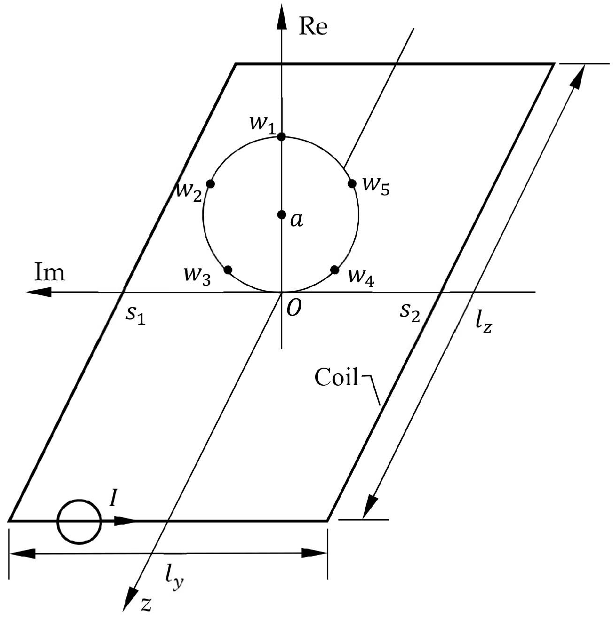
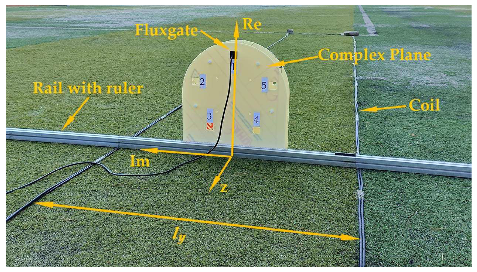
As shown in Figure 12, a rectangular coil is placed on the ground, with the long side $l_z$ = 10.5 m and the short side $l_y$ = 1 m. In order to avoid the influence of the fluctuation of the magnetic field in the urban area, a sinusoidal current with an amplitude of 14.4 A and a frequency of 10 Hz is introduced into the coil. Then, the magnetic field generated by the sinusoidal current can be separated by Fourier transform.

Figure 12. Measurement of the fractional derivative on survey line by the TR series. The symbols Re and Im indicate the real axis and the imaginary axis respectively, and the symbol z denote the z-axis. The symbol $l_y$ is the distance between two long sides, and it is also the length of the short sides.

The yellow board is in the complex plane. It is perpendicular to the long sides and at the center of the long sides. The real axis is vertical, and the imaginary axis is horizontal. The radius of the circle $C$ is 0.17 m. Five holes $w_1~w_5$ are uniformly distributed on the circle $C$ to hold the fluxgate sensor. The start point $b$ is on the circle $C$, and the end point $a$ is the center of the circle.

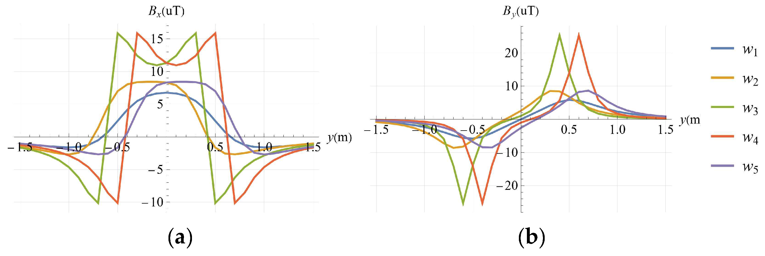
The survey line is horizontal and 0.25 m above the ground. We use the aluminum rail with a ruler attached to indicate the horizontal position on the survey line. The center $a$ of the circle $C$ is on the survey line, and its range of movement on the survey line is (−1.5 m, 1.5 m). The distance between the survey points is 0.1 m. Then, the measurement is performed, and the magnetic field components $B_x$, $B_y$ measured at each survey point $w_n$ are shown in Figure 13.

Figure 13. Magnetic field components measured at $w_n$. Field components: (a) $B_x$; (b) $B_y$.

We also plot the exact values in Figure 14 for comparison.

Figure 14. Exact values of the magnetic field component at each $w_n$. Field components: (a) $B_x$; (b) $B_y$.

We find that the measured values near y = ±0.5 m where the current is located are larger than expected. This is because the magnetic field changes rapidly near the current as shown in Figure 14b, and a small position error can cause significant changes in the measured values.

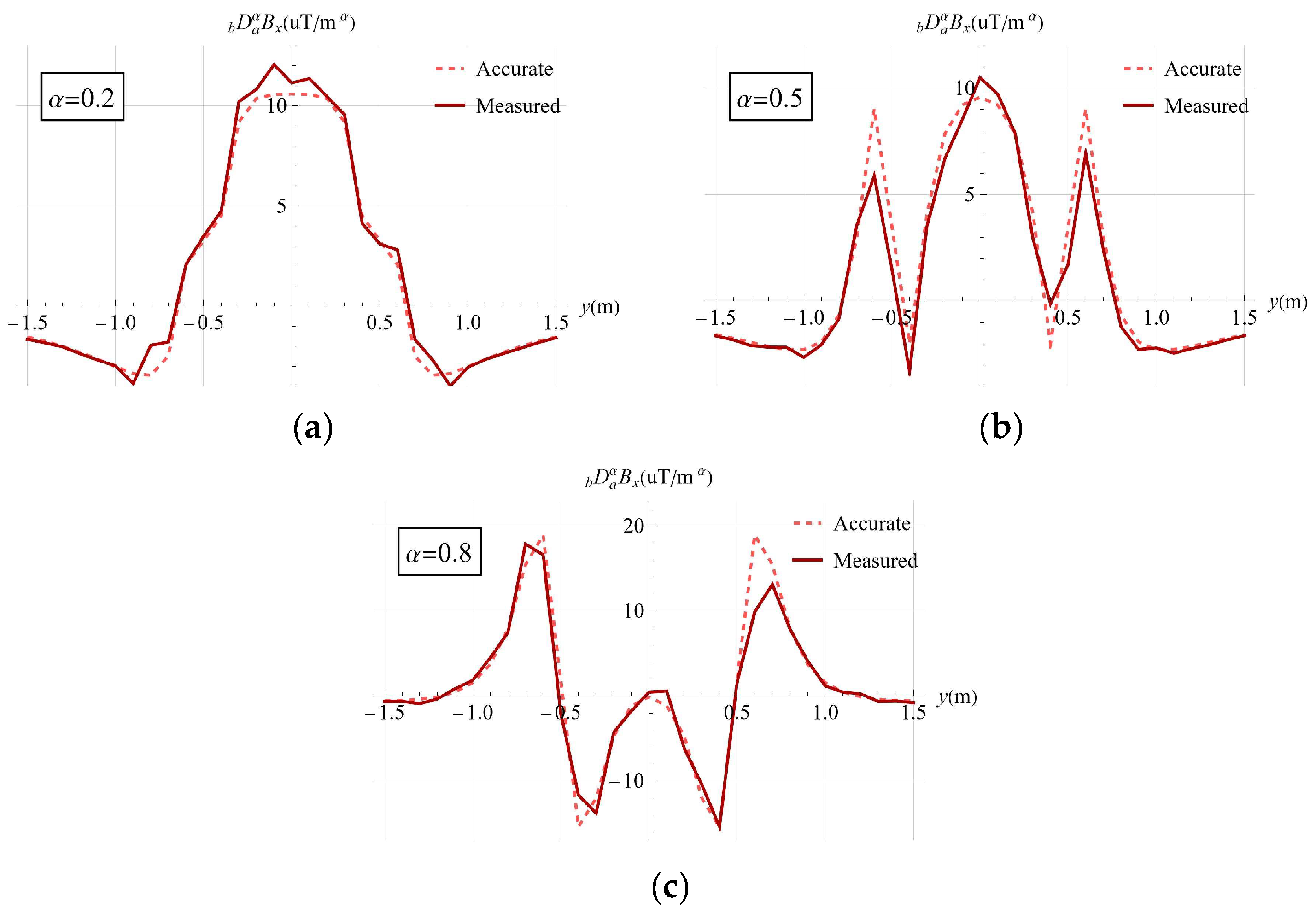
Then, we calculate ${{}_{b}D}_a^{\alpha }{B}_x$ with the order of $\alpha$ = 0.2, 0.5, 0.8 according to (3). The results are shown in Figure 15.

Figure 15. Measured and accurate value of ${{}_{b}D}_a^{\alpha }{B}_x$ with the derivative order of: (a) $\alpha$ = 0.2; (b) $\alpha$ = 0.5; (c) $\alpha$ = 0.8.

The calculated result is close to the analytical result. Therefore, the TR method is valid for fractional derivative measurement and can suppress the noise.

5. Conclusions

In this article, a method for measuring the fractional derivative of the two-dimensional magnetic field is derived by using the Taylor–Riemann series and the analytic function of the two-dimensional magnetic field. The simulation and experiment show the effectiveness of this method. Furthermore, this method can effectively suppress Gaussian noise, and it is possible to obtain fractional derivatives in real time from a few survey points.

References

1. Miller, K.S.; Ross, B. An Introduction to the Fractional Calculus and Fractional Differential Equations; Wiley: New York, NY, USA, 1993; pp. 1–3. [Google Scholar]
2. Miah, B.A.; Sen, M.; Murugan, R.; Gupta, D. Developing Riemann–Liouville-Fractional Masks for Image Enhancement. Circ. Syst. Signal Process. 2024, 43, 3802–3831. [Google Scholar] [CrossRef]
3. Hassan, S.K.; Ali Alazzawi, S.N.; Ibrahem, N.M.J. Some Results in Grunwald-Letnikov Fractional Derivative and its Best Approximation. J. Phys. Conf. Ser. 2021, 1818, 012020. [Google Scholar] [CrossRef]
4. Caputo, M. Linear models of dissipation whose Q is almost frequency independent-II. Geophys. J. Int. 1967, 13, 529–539. [Google Scholar] [CrossRef]
5. Atangana, A.; Gomez-Aguilar, J.F. Fractional derivatives with no-index law property: Application to chaos and statistics. Chaos Solit. Fract. 2018, 114, 516–535. [Google Scholar] [CrossRef]
6. Atangana, A. Non-validity of index law in fractional calculus: A fractional differential operator with Markovian and non-Markovian properties. Physica A 2018, 505, 688–706. [Google Scholar] [CrossRef]
7. Bouzeffour, F. Advancing Fractional Riesz Derivatives through Dunkl Operators. Mathematics 2023, 11, 4073. [Google Scholar] [CrossRef]
8. Ho, K.P. Modular Hadamard, Riemann-Liouville and Weyl fractional integral. Mathematica 2023, 65, 263–274. [Google Scholar] [CrossRef]
9. Podlubny, I. Fractional Differential Equations; Academic Press: San Diago, CA, USA, 1999; p. 42. [Google Scholar]
10. Lavoie, J.L.; Osler, T.J.; Tremblay, R. Fractional Derivatives and Special Functions. SIAM Rev. 1976, 18, 240–268. [Google Scholar] [CrossRef]
11. Has, A.; Yılmaz, B. Effect of fractional analysis on magnetic curves. Rev. Mex. Fis. 2022, 68, 041401. [Google Scholar] [CrossRef]
12. Weiss, C.J.; van Bloemen Waanders, B.G.; Antil, H. Fractional operators applied to geophysical electromagnetics. Geophys. J. Int. 2020, 220, 1242–1259. [Google Scholar] [CrossRef]
13. Ge, J.; Everett, M.E.; Weiss, C.J. Fractional diffusion analysis of the electromagnetic field in fractured media—Part 2: 3D approach. Geophysics 2015, 80, E175–E185. [Google Scholar] [CrossRef]
14. Podlubny, I. Geometric and Physical Interpretation of Fractional Integration and Fractional Differentiation. Fract. Calc. Appl. Anal. 2002, 5, 367–386. [Google Scholar]
15. Bai, L.; Xue, D.Y. Geometric Meaning of a Special Riemann-Liouville Fractional-Order Integral. MIPAT 2020, 50, 234–239. [Google Scholar]
16. Peters, L.J. The direct approach to magnetic interpretation and its practical application. Geophysics 1949, 14, 290–320. [Google Scholar] [CrossRef]
17. Gunn, P.J. Linear transformations of gravity and magnetic fields. Geophys. Prospect. 1975, 23, 300–312. [Google Scholar] [CrossRef]
18. Gunn, P.J.; Fitzgerald, D.; Yassi, N.; Dart, P. New algorithms for visually enhancing airborne geophysical data. Explor. Geophys. 1997, 28, 220–224. [Google Scholar] [CrossRef]
19. Cooper, G.; Cowan, D. The application of fractional calculus to potential field data. Explor. Geophys. 2003, 34, 51–56. [Google Scholar] [CrossRef]
20. Oldham, K.B.; Spanier, J. The Fractional Calculus; Academic Press: San Diego, CA, USA, 1974; pp. 48–51. [Google Scholar]
21. Cooper, G.R.J.; Cowan, D.R. Sunshading geophysical data using fractional order horizontal gradients. TLE 2003, 22, 204–205. [Google Scholar] [CrossRef]
22. Cowan, D.; Cooper, G. Separation filtering using fractional order derivatives. Explor. Geophys. 2005, 36, 393–396. [Google Scholar] [CrossRef]
23. Arısoy, M.O.; Dikmen, U. Edge enhancement of magnetic data using fractional-order-derivative filters. Geophysics 2015, 80, J7–J17. [Google Scholar] [CrossRef]
24. Hood, P. Gradient measurements in aeromagnetic surveying. Geophysics 1965, 30, 891–902. [Google Scholar] [CrossRef]
25. Stolz, R.; Zakosarenko, V.; Schulz, M.; Chwala, A.; Fritzsch, L.; Meyer, H.G.; Köstlin, E.O. Magnetic full-tensor SQUID gradiometer system for geophysical applications. Lead. Edge 2006, 25, 178–180. [Google Scholar] [CrossRef]
26. Pei, Y.H.; Yeo, H.G.; Kang, X.Y.; Pua, S.L.; Jhon, T. Magnetic gradiometer on an AUV for buried object detection. In OCEANS 2010 MTS/IEEE SEATTLE; IEEE: Seattle, WA, USA, 2010. [Google Scholar]
27. Cocchi, L.; Carmisciano, C.; Palangio, P.; Gualdesi, L. S3MAG-Low Magnetic Noise AUV for Multipurpose Investigations Oceans; IEEE: Genova, Italy, 2015. [Google Scholar]
28. Chen, J.F. Research on Method of Magnetic Anomaly Detection Based on Gradient Tensor. Ph.D. Thesis, National University of Defense Science and Technology, Changsha, China, 2012. [Google Scholar]
29. Sunderland, A.; Ju, L.; Blair, D.G.; McRae, W.; Veryaskin, A.V. Optimizing a direct string magnetic gradiometer for geophysical exploration. Rev. Sci. Instrum. 2009, 80, 104705. [Google Scholar] [CrossRef]
30. Tilbrook, D.L. Rotating magnetic tensor gradiometry and a superconducting implementation. Supercond. Sci. Technol. 2009, 22, 075002. [Google Scholar] [CrossRef]
31. Munkhammar, J. Riemann-Liouville Fractional Derivatives and the Taylor-Riemann Series. Ph.D. Thesis, Uppsala University, Uppsala, Sweden, June 2004. [Google Scholar]
32. Xue, D.Y. Fractional Calculus and Fractional-Order Control; Science Press: Beijing, China, 2018; pp. 63–64. [Google Scholar]
33. Hardy, G.H. Riemann’s form of Taylor’s series. J. Lond. Math. Soc. 1945, 20, 48–57. [Google Scholar] [CrossRef]
34. Osler, T.J. Leibniz Rule, the Chain Rule, and Taylor’s Theorem for Fractional Derivatives. Ph.D. Thesis, New York University, New York, NY, USA, 1970. [Google Scholar]
35. Lapidoth, A. A Foundation in Digital Communication, 2nd ed.; Cambridge University Press: Cambridge, UK, 2017; pp. 314–340. [Google Scholar]