Article

Dengue Transmission Dynamics: A Fractional-Order Approach with Compartmental Modeling

1
Department of Mathematics, College of Science, Jazan University, P.O. Box 114, Jazan 45142, Saudi Arabia
2
Department of Mathematics and Statistics, The University of Lahore, Lahore 54000, Pakistan
*
Author to whom correspondence should be addressed.
Fractal Fract. 2024, 8(4), 207; https://doi.org/10.3390/fractalfract8040207
Submission received: 23 February 2024 / Revised: 27 March 2024 / Accepted: 28 March 2024 / Published: 2 April 2024

Abstract

:
This work presents a quantitative analysis of the transmission dynamics of dengue using the Caputo–Fabrizio fractional-order derivative. It presents an extensive framework for modeling a dengue epidemic, including the various stages of infection and encompassing a wide range of transmission pathways. The proposed model is subjected to a rigorous qualitative study, including the determination of a non-negative solution, the assessment of the basic reproduction number, and an evaluation of local stability. Numerical solutions are obtained using the Newton method. The fractional-order operator, developed using the Caputo–Fabrizio approach, provides a refined perspective on the transmission dynamics of dengue. This study contributes to a deeper understanding of the disease’s transmission mechanisms, considering both fractional-order dynamics and diverse transmission routes, thus offering insights for enhanced disease management and control.

1. Introduction

Dengue, an infectious disease caused by the dengue virus and transmitted by Aedes mosquitoes, is a significant public health issue due to the absence of definitive therapeutic interventions and its rank as the most prevalent arboviral disease worldwide. It remains a significant global health concern, with an approximate annual incidence of 390 million infections [1]. The estimated number of apparent cases in 1990 was 8.3 million, ranging from 3.3 million to 17.2 million. This estimate increased to 58.4 million by 2013, ranging from 23.6 million to 121.9 million [2]. Following infection, there is a variable period of incubation lasting between 3 and 10 days before the appearance of distinct symptoms, including severe headaches, joint pain, muscle pain, skin rashes, and hemorrhagic manifestations [3]. Comprehending the extensive influence of dengue on worldwide health and acknowledging its clinical manifestation is crucial in formulating efficacious preventive strategies and potential therapeutic interventions. Most instances present as uncomplicated dengue fever (DF), but some individuals may advance to the more severe form known as dengue hemorrhagic fever (DHF). Plasma leakage characterizes DHF and typically manifests shortly after the febrile phase. In certain instances, the disease has the potential to progress to dengue shock syndrome (DSS), a potentially life-threatening condition characterized by severe plasma leakage resulting in hypovolemic shock [4]. The current global fatality rate associated with dengue fever is below 0.4% [5].
Nevertheless, obtaining precise data regarding global mortality rates is challenging. Approximations indicate an annual average of 9221 deaths attributed to dengue between 1990 and 2013 [5]. It is worth noting that dengue outbreaks demonstrate unpredictable patterns, further intensifying the burden on healthcare facilities and resulting in overcrowded hospitals and strained resources. It is imperative to comprehend dengue fever’s diverse clinical manifestations and worldwide ramifications to develop efficacious approaches for managing and preventing this disease. There needs to be more established methodologies for forecasting dengue outbreaks. If these outbreaks could be reliably predicted, it would be possible to implement suitable preventive measures proactively. Furthermore, it is crucial to notify health services in advance, allowing them to proactively implement essential measures to accommodate the anticipated surge of individuals seeking treatment for dengue during these outbreaks. Multiple meteorological variables, such as temperature, humidity, precipitation, and wind speed, substantially impact mosquito population density [6]. Favorable meteorological conditions contribute to an upsurge in mosquito population density, as heightened precipitation exacerbates the accumulation of sewage and overwhelms waste management systems in numerous geographical areas. As a result, the optimal breeding habitats of dengue mosquitoes are in regions characterized by water accumulation, particularly in periods of increased precipitation.
Furthermore, a dense human population amplifies the challenges associated with waste disposal, thereby leading to additional breeding sites. The presence of the dengue virus in the environment, in conjunction with the density of mosquitoes, significantly influences the prevalence of mosquitoes capable of transmitting the virus [7]. Elevated temperatures have the dual effect of promoting the desiccation of running water sources and facilitating the formation of stagnant water reservoirs. The ideal conditions for the dengue mosquito to complete its life cycle are found in these stagnant ponds. On the other hand, some mosquito larvae may become vulnerable in too-hot environments [8]. This observation suggests that temperature can positively and negatively influence mosquito density and the incidence of dengue cases. Comprehending these intricate interactions is imperative in formulating efficacious strategies for predicting and preventing dengue outbreaks.
For several years, epidemiological research has utilized significant mathematical models [9,10]. In order to make the elements involved in the interactions among hosts, vectors, and pathogens more clear, these models serve as formal frameworks. Epidemic models are essential tools used to understand and forecast the dynamics of infectious diseases in different scenarios. They are commonly utilized to evaluate the effectiveness of public health interventions in disease control. In the scientific literature, dengue fever’s epidemiological dynamics have been represented mathematically since 1970 [11]. Dengue fever is a prominent illustration of a viral infection transmitted by mosquitoes, presenting a significant global public health issue. Most instances of the disease present with no symptoms or only mild symptoms [12,13]. However, severe cases of the disease are caused by various serotypes, and a significant mechanism contributing to this severity is antibody-dependent enhancement (ADE). Antibody-dependent enhancement (ADE) refers to a phenomenon in which pre-existing antibodies are unable to effectively neutralize a novel infection and instead exacerbate its effects.
The goal of dengue fever mathematical models is to correctly capture the intricate epidemiological dynamics of the illness while taking into account a variety of aspects related to the disease and its vectors. Consequently, even the most basic dynamical models have been found to exhibit a vast diversity of dynamic behaviors. These models have been specifically developed to assess crucial factors, including the simultaneous presence of multiple strains or variants, the immunological mechanisms contributing to the disease’s severity, and the potential effects of vaccination. This concept resembles the current approaches employed in comprehending the epidemiology of COVID-19. Mathematical models are crucial in informing public health policies and strategies for controlling and preventing dengue fever by integrating various aspects of the disease. Fractional calculus, an extension of classical calculus, introduces the concept of fractional derivatives, which proves valuable in enhancing our understanding of diverse phenomena. Models incorporating non-integer-order operators offer improved precision in capturing phenomena characterized by disintegrating memory and inversion behavior. Particularly in the context of diseases under investigation, including fractional derivatives provides additional insights [14,15,16,17,18,19]. Within the existing literature, various fractional operators featuring both nonsingular and singular kernels have been proposed [20,21,22,23]. A comprehensive examination of these fractional-order operators and their applications is available in [24,25,26,27]. Using fractional calculus in mathematical models offers a promising avenue for advancing our comprehension of intricate biological processes and disease dynamics. This paper extends the prior research conducted by the author [28], which centered on a mathematical model exclusively addressing the dengue class. In contrast, the current investigation incorporates novel variants within the dengue class and assesses the consequences of their co-infection.

2. Mathematical Modeling

2.1. Preliminaries on Fractional Derivatives

In this section, we provide a concise overview of key concepts pertaining to fractional derivatives, with the aim of facilitating comprehension for our audience. A comprehensive analysis of this novel facet of calculus can be found in [29].
Definition 1. 
Suppose a function g : R + R for ζ > 0 . Then, the upper and lower Riemann–Liouville fractional integrals for the closed interval [ α , β ] are defined by
D t ζ α R L = I t ζ α R L = 1 Γ ( ζ ) α t ( t x ) ζ 1 g ( x ) d x , f o r t > α , D β ζ t R L = I β ζ t R L = 1 Γ ( ζ ) t b ( x t ) ζ 1 g ( x ) d x , f o r t < β ,
where Γ is the gamma function.
Definition 2. 
Suppose a function g : R + R . Then, the upper and lower Riemann–Liouville fractional derivatives are defined as [30]
D t ζ a R L g ( t ) = d n d t n D t ( n ζ ) a R L g ( t ) = d n d t n I t n ζ a R L g ( t ) ,
D b ζ t R L g ( t ) = d n d t n D b ( n ζ ) t R L g ( t ) = d n d t n I b n ζ t R L g ( t ) ,
Definition 3. 
Caputo [31] proposed an alternative definition of the Riemann–Liouvile derivative to address certain limitations, which is given by
D t ζ 0 C g ( t ) = 1 Γ ( n ζ ) 0 t g ( n ) ( Ψ ) ( t Ψ ) ζ n + 1 d Ψ ,
where ζ ( n 1 , n ) and n N . Obviously, D t ζ 0 C g ( t ) D t ζ g ( t ) whenever ζ 1 . Thus, D t ζ 0 C g ( t ) and D t ζ h ( t ) exist almost everywhere. Let s 1 , s 2 R . Then, D t ζ 0 C [ s 1 g ( t ) + s 2 h ( t ) ] exists almost everywhere with
D t ζ 0 C [ s 1 g ( t ) + s 2 h ( t ) ] = s 1 [ 0 C D t ζ g ( t ) ] + s 2 [ 0 C D t ζ h ( t ) ] .
Definition 4. 
The equilibrium point, denoted as C * , for the Caputo system can be defined as
D t ζ 0 C C * ( t ) = g ( t , C * ( t ) ) g ( t , C * ( t ) ) = 0 , w h e r e 0 < ζ > 1 .
Definition 5. 
Consider the Sobolev space H 1 ( a , b ) and g H 1 ( a , b ) , b > a , ζ [ 0 , 1 ] , defined as
H 1 ( a , b ) = g L 2 ( a , b ) : D g L 2 ( a , b ) .
The Caputo fractional derivative in this case is defined as [32]
D t ζ 0 C g ( t ) = M ( ζ ) 1 ζ a t D t ζ g ( x ) e x p [ ζ t x 1 ζ ] d y ,
where M ( ζ ) is the normalization function such that M ( 0 ) = M ( 1 ) = 1 .
Definition 6. 
The Caputo–Fabrizio fractional derivative for the function g ( t ) is defined as
D t ζ 0 C F g ( t ) = M ( ζ ) 1 ζ a t ( g ( t ) g ( x ) ) e x p [ ζ t x 1 ζ ] d y .

2.2. Mathematical Model of Dengue

2.2.1. Classical Integer Model

The classical integer model of co-infection epidemic between humans and mosquitoes is given below:
  • Human populations
D S h = Λ h β ( I v S h ) d h S h + δ R h + ϵ V h ,
D E h = β ( I v S h ) ( γ h + d h + η ) E h ,
D I h = γ h E h ( η + q 1 + d h ) I h ,
D V h = γ h S h ( ϵ + α + d h ) V h ,
D P h = η I h + η E h ( δ + q 2 + d h ) P h ,
D R h = q 1 I h + q 2 P h d h R h δ R h + α V h .
  • Vector populations
D S v = Λ v β ( I h S v ) d v S v ,
D E v = β ( I h S v ) ( γ v + d v ) E v ,
D I v = γ v E V d v I v .
The initial conditions are
S h = S h ( 0 ) , E h = 0 , I h = 0 , V h = 0 , P h = 0 , R h = 0 , S v = S v ( 0 ) , E v = 0 , I v = 0

2.2.2. Caputo–Fabrizio Fractional Derivative

In this subsection, we modify the classical integer model into the fractional-order model in the Caputo–Fabrizio sense.
  • Human populations
D t ζ 0 C F S h = Λ h β ( I v S h ) d h S h + δ R h + ϵ V h , D t ζ 0 C F E h = β ( I v S h ) ( γ h + d h + η ) E h , D t ζ 0 C F I h = γ h E h ( η + q 1 + d h ) I h , D t ζ 0 C F V h = γ h S h ( ϵ + α + d h ) V h , D t ζ 0 C F P h = η I h + η E h ( δ + q 2 + d h ) P h , D t ζ 0 C F R h = q 1 I h + q 2 P h d h R h δ R h + α V h ,
  • Vector populations
D t ζ 0 C F S v = Λ v β ( I h S v ) d v S v , D t ζ 0 C F E v = β ( I h S v ) ( γ v + d v ) E v , D t ζ 0 C F I v = γ v E V d v I v ,
The description of the parameters is given in Table 1.

3. Numerical Simulations and Analysis of the Model

3.1. Existence and Uniqueness

For the given model’s well-posedness, the theorem stating that its solution is never negative is shown below.
Theorem 1 
(Non-Negativity Criteria). The solution of the proposed dengue model is contained in the interval [ 0 , ) and { S h ( t ) , E h ( t ) , I h ( t ) , V h ( t ) , P h ( t ) , R h ( t ) , S v ( t ) , E v ( t ) , I v ( t ) } 0 for all values of 0 t < .
Proof. 
All the right-hand sides of the proposed model are completely continuous and locally Lipschitzian on R 0 9 . The solutions of { S h ( t ) , E h ( t ) , I h ( t ) , V h ( t ) , P h ( t ) , R h ( t ) , S v ( t ) , E v ( t ) , I v ( t ) } with initial conditions exist and are unique in the interval [ 0 , ) [33].
From Equation (1), where [ Λ h β ( I v S h ) + δ R h + ϵ V h ] 0 , we obtain the following viable inequality
d S h d t d h S h ,
This implies that
S h ( t ) S h ( 0 ) e d h ( t ) 0 .
This guarantees that its derivative exhibits an upward trend whenever the solution approaches the axis, and the function S h ( t ) remains in the positive domain. From Equation (2), we have
d E h d t ( ϕ 2 ) E h ,
E h ( t ) E h ( 0 ) e ( ϕ 2 ) ( t ) 0 .
This guarantees that its derivative exhibits an upward trend whenever the solution approaches the axis, and the function E h ( t ) remains in the positive domain. Similarly, when we solve the remaining equations, we obtain
I h ( t ) I h ( 0 ) e ( ϕ 3 ) ( t ) 0 ,
V h ( t ) V h ( 0 ) e ( ϕ 1 ) ( t ) 0 ,
P h ( t ) p h ( 0 ) e ( ϕ 4 ) ( t ) 0 ,
R h ( t ) R h ( 0 ) e ( d h + δ ) ( t ) 0 ,
S v ( t ) S v ( 0 ) e ( d v ( t ) ) 0 ,
E v ( t ) E v ( 0 ) e ( ϕ 5 ( t ) ) 0 ,
I v ( t ) I v ( 0 ) e ( d v ( t ) ) 0 .
Hence, I h ( t ) , V h ( t ) , P h ( t ) , R h ( t ) , S v ( t ) , E v ( t ) , I v ( t ) is a function that is non-negative for all values of t [ 0 , ) .

3.2. Stability Analysis

The concept of stability by the disease-free equilibrium is used to examine the co-infection of the model.

3.2.1. Disease-Free Equilibrium Point

We calculate the following equilibrium point:
E 0 = ( S h , E h , I h , V h , P h , R h , S v , E v , I v ) = ( Λ h ( ϵ + α + d h ) ϵ γ h + ϵ d h + α d h + d h 2 , 0 , 0 , Λ h γ h ϵ γ h + ϵ d h + α d h + d h 2 , 0 , 0 , Λ v d v , 0 , 0 )

3.2.2. Reproductive Number

The next-generation matrices are calculated as
F = 0 0 0 0 β S h 0 0 0 0 0 0 0 0 0 0 0 β S v 0 0 0 0 0 0 0 0 , V = γ h + d h + η 0 0 0 0 γ h η + q 1 + d h 0 0 0 η η δ + q 2 + d h 0 0 0 0 0 γ v + d v 0 0 0 0 γ v d v .
The reproductive number can be calculated as
R 0 = ρ ( F V 1 ) ,
R 0 = β 4 Λ v γ h γ v Λ h T 44 T 33 T 22 T 88 ( d h 2 + ( α + ϵ ) d h + γ h ϵ ) d v 4 ,
where T 22 = ( γ h + d h + η ) , T 33 = ( η + q 1 + d h ) , T 44 = ( ϵ + α + d h ) , and T 88 = ( γ v + d v ) .
Theorem 2 
(Stability Analysis). The disease-free equilibrium point ( E 0 ) is locally asymptotically stable if R 0 < 1 and unstable if R 0 > 1 .
Proof. 
The Jacobian matrix at ( E 0 ) is given by
J | 0 | = d h 0 0 ϵ 0 δ 0 0 β Λ h ( ϵ + α + d h ) ϵ γ h + ϵ d h + α d h + d h 2 0 T 22 0 0 0 0 0 0 β Λ h ( ϵ + α + d h ) ϵ γ h + ϵ d h + α d h + d h 2 0 γ h T 33 0 0 0 0 0 γ h 0 0 T 44 0 0 0 0 0 0 η η 0 T 55 0 0 0 0 0 0 q 1 α q 2 T 66 0 0 0 0 0 β Λ v d v 0 0 0 d v 0 0 0 0 β Λ v d v 0 0 0 0 T 88 0 0 0 0 0 0 0 0 γ v d v ,
where T 55 = ( δ + q 2 + d h ) , T 66 = ( d h + d v ) , T 88 = ( γ v + d v ) . According to [34], if all eigenvalues of the Jacobian matrix are strictly in the left-half complex plane, the equilibrium point is locally asymptotically stable. The eigenvalues of the given Jacobian matrix are as follows
λ 1 = d v , λ 2 = T 55 , λ 3 = T 22 , λ 4 = T 33 , λ 5 = T 88 , λ 6 = d h ,
λ 7 = T 44 d h ϵ γ h d h , λ 8 = T 66 T 44 d h T 66 ϵ γ h α Δ γ h T 44 d h ϵ γ h ,
λ 9 = β 2 γ h γ v Λ h Λ v T 44 T 22 T 33 T 88 ( d h 2 + ( ϵ + α ) d h + ϵ γ h ) d v 2 .
This shows that the disease-free equilibrium is locally asymptotically stable if R 0 < 1 and unstable if R 0 > 1 . λ 3 = T 22 , λ 4 = T 33 , λ 5 = T 88 , λ 6 = d h , λ 7 = T 44 d h ϵ γ h d h , and
λ 8 = T 66 T 44 d h T 66 ϵ γ h α Δ γ h T 44 d h ϵ γ h . So, the six eigenvalues of J 2 | 0 | are negative The last one also includes a negative sign if λ 9 = β 2 γ h γ v Λ h Λ v T 44 T 22 T 33 T 88 ( d h 2 + ( ϵ + α ) d h + ϵ γ h ) d v 2 < 0 and β 4 γ h γ v Λ h Λ v T 44 T 22 T 33 T 88 ( d h 2 + ( ϵ + α ) d h + ϵ γ h ) d v 4 < 1 . Hence, it is locally asymptotically stable if R 0 < 1 . □

3.3. Discrete Scheme for Caputo–Fabrizio Fractional Derivative

The Cauchy problem is given as
D t ζ 0 C F h ( t ) = g ( t , h ( t ) ) , h ( 0 ) = h 0
where the derivative is the Caputo–Fabrizio derivative. We use the Newton method to solve Equation (24). For this, we first transform Equation (24) into
h ( t ) h ( 0 ) = 1 ζ M ( ζ ) g ( t , h ( t ) ) + ζ M ( ζ ) 0 t g ( X , h ( X ) ) d X .
At t i + 1 = ( i + 1 ) Δ t , we have
h ( t i + 1 ) h ( 0 ) = 1 ζ M ( ζ ) g ( t i , h ( t i ) ) + ζ M ( ζ ) 0 t i + 1 g ( X , h ( X ) ) d X .
At t i = i Δ t , we have
h ( t i ) h ( 0 ) = 1 ζ M ( ζ ) g ( t i 1 , h ( t i 1 ) ) + ζ M ( ζ ) 0 t i g ( X , h ( X ) ) d X .
From Equations (26) and (27), we obtain
h ( t i + 1 ) h ( t i ) = 1 ζ M ( ζ ) G 3 + ζ M ( ζ ) n = 2 i t i t i + 1 g ( X , h ( X ) ) d X ,
and
h ( t i + 1 ) h ( t i ) = 1 ζ M ( ζ ) G 3 + ζ M ( ζ ) n = 2 i t n t n + 1 g ( X , h ( X ) ) d X .
We use the Newton polynomial to approximate the function g ( t , h ( t ) ) , as follows
Q i ( X ) = g ( ( t i 2 ) , h ( t i 2 ) ) + G 4 Δ ( t ) ( X t i 2 ) + G 5 2 Δ ( t 2 ) ( X t i 2 ) ( X t i 1 ) ,
where
G 3 = g ( t i 2 , h ( t i ) ) g ( t i 1 , h ( t i 1 ) ) , G 4 = g ( t i 1 , h ( t i 1 ) ) g ( t i 2 , h ( t i 2 ) ) , G 5 = g ( t i , h ( t i ) ) 2 g ( t i 1 , g ( t i 1 ) ) + g ( t i 2 , g ( t i 2 ) ) .
Thus, using Equations (29) and (30), we obtain
h i + 1 h 0 = 1 ζ M ( ζ ) G 3 + ζ M ( ζ ) n = 2 i t n t n + 1 { g ( t n 1 , h n 2 ) + G 1 Δ t × ( X t n 2 ) + G 2 2 Δ t 2 × ( X t n 2 ) ( X t n 1 ) } d X .
After simplification, we obtain
h i + 1 h 0 = 1 ζ M ( ζ ) G 3 + ζ M ( ζ ) n = 2 i { g ( t n 2 , h n 2 ) t n t n + 1 d X + 1 Γ ( ζ ) n = 2 i t n t n + 1 G 1 Δ t ( X t n 2 ) d X + 1 Γ ( ζ ) n = 2 i G 2 2 Δ t 2 t n t n + 1 ( X t n 2 ) ( X t n 1 ) d X } .
The calculations for the above integrals in Equation (32) are as follows
t n t n + 1 ( X t n 2 ) d X = 5 2 Δ t 2 ,
t n t n + 1 ( X t n 2 ) ( X t n 1 ) d X = 23 6 Δ t 3
Now, by substituting the expressions from Equations (33) and (34) into (32), we obtain
h i + 1 = h 0 + 1 ζ M ( ζ ) G 3 + ζ M ( ζ ) n = 2 i t n t n + 1 { g ( t n 2 , h n 2 ) + G 4 5 2 + G 5 23 6 } Δ t d X ,
and we can arrange it as
h i + 1 = h 0 + 1 ζ M ( ζ ) G 3 + ζ M ( ζ ) n = 2 i t n t n + 1 { ( 32 12 g ( t n , h n ) 4 3 g ( t n 1 , g n 1 ) + 5 12 g ( t n 2 , h n 2 ) ) × ( t n + 1 t n ) } d X .
By using the above equation and applying the Caputo–Fabrizio derivative, the proposed model has the following discrete scheme [35]
S h ( t i + 1 ) = S h ( t i ) + 1 ζ M ( ζ ) [ δ 1 δ 10 ] + ζ M ( ζ ) n = 2 j { ( 23 12 δ 1 4 3 δ 10 + 5 12 δ 19 ) Δ t } .
E h ( t i + 1 ) = E h ( t i ) + 1 ζ M ( ζ ) [ δ 2 δ 11 ] + ζ M ( ζ ) n = 2 j { ( 23 12 δ 2 4 3 δ 11 + 5 12 δ 20 ) Δ t } .
I h ( t i + 1 ) = I h ( t i ) + 1 ζ M ( ζ ) [ δ 3 δ 12 ] + ζ M ( ζ ) n = 2 j { ( 23 12 δ 3 4 3 δ 12 + 5 12 δ 21 ) Δ t } .
V h ( t i + 1 ) = V h ( t i ) + 1 ζ M ( ζ ) [ δ 4 δ 10 ] + ζ M ( ζ ) n = 2 j { ( 23 12 δ 4 4 3 δ 13 + 5 12 δ 22 ) Δ t } .
P h ( t i + 1 ) = P h ( t i ) + 1 ζ M ( ζ ) [ δ 5 δ 13 ] + ζ M ( ζ ) n = 2 j { ( 23 12 δ 5 4 3 δ 14 + 5 12 δ 23 ) Δ t } .
R h ( t i + 1 ) = R h ( t i ) + 1 ζ M ( ζ ) [ δ 6 δ 15 ] + ζ M ( ζ ) n = 2 j { ( 23 12 δ 6 4 3 δ 15 + 5 12 δ 24 ) Δ t } .
S v ( t i + 1 ) = S v ( t i ) + 1 ζ M ( ζ ) [ δ 7 δ 16 ] + ζ M ( ζ ) n = 2 j { ( 23 12 δ 7 4 3 δ 16 + 5 12 δ 25 ) Δ t } .
E v ( t i + 1 ) = E v ( t i ) + 1 ζ M ( ζ ) [ δ 8 δ 17 ] + ζ M ( ζ ) n = 2 j { ( 23 12 δ 8 4 3 δ 17 + 5 12 δ 26 ) Δ t } .
I v ( t i + 1 ) = I v ( t i ) + 1 ζ M ( ζ ) [ δ 9 δ 18 ] + ζ M ( ζ ) n = 2 j { ( 23 12 δ 9 4 3 δ 18 + 5 12 δ 27 ) Δ t } .
where , δ 1 = S h 1 ( ( t i ) , S h ( t i ) , E h ( t i ) , I h ( t i ) , V h ( t i ) , P h ( t i ) , R h ( t i ) , S v ( t i ) , E v ( t i ) , I v ( t i ) ) , δ 2 = E h 1 ( ( t i ) , S h ( t i ) , E h ( t i ) , I h ( t i ) , V h ( t i ) , P h ( t i ) , R h ( t i ) , S v ( t i ) , E v ( t i ) , I v ( t i ) ) , δ 3 = I h 1 ( ( t i ) , S h ( t i ) , E h ( t i ) , I h ( t i ) , V h ( t i ) , P h ( t i ) , R h ( t i ) , S v ( t i ) , E v ( t i ) , I v ( t i ) ) , δ 4 = V h 1 ( ( t i ) , S h ( t i ) , E h ( t i ) , I h ( t i ) , V h ( t i ) , P h ( t i ) , R h ( t i ) , S v ( t i ) , E v ( t i ) , I v ( t i ) ) , δ 5 = P h 1 ( ( t i ) , S h ( t i ) , E h ( t i ) , I h ( t i ) , V h ( t i ) , P h ( t i ) , R h ( t i ) , S v ( t i ) , E v ( t i ) , I v ( t i ) ) , δ 6 = R h 1 ( ( t i ) , S h ( t i ) , E h ( t i ) , I h ( t i ) , V h ( t i ) , P h ( t i ) , R h ( t i ) , S v ( t i ) , E v ( t i ) , I v ( t i ) ) , δ 7 = S v 1 ( ( t i ) , S h ( t i ) , E h ( t i ) , I h ( t i ) , V h ( t i ) , P h ( t i ) , R h ( t i ) , S v ( t i ) , E v ( t i ) , I v ( t i ) ) , δ 8 = E v 1 ( ( t i ) , S h ( t i ) , E h ( t i ) , I h ( t i ) , V h ( t i ) , P h ( t i ) , R h ( t i ) , S v ( t i ) , E v ( t i ) , I v ( t i ) ) , δ 9 = I v 1 ( ( t i ) , S h ( t i ) , E h ( t i ) , I h ( t i ) , V h ( t i ) , P h ( t i ) , R h ( t i ) , S v ( t i ) , E v ( t i ) , I v ( t i ) ) , δ 10 = S h 1 ( t i 1 , S h ( t i 1 ) , E h ( t i 1 ) , I h ( t i 1 ) , V h ( t i 1 ) , P h ( t i 1 ) , R h ( t i 1 ) , S v ( t i 1 ) , E v ( t i 1 ) , I v ( t i 1 ) ) , δ 11 = E h 1 ( t i 1 , S h ( t i 1 ) , E h ( t i 1 ) , I h ( t i 1 ) , V h ( t i 1 ) , P h ( t i 1 ) , R h ( t i 1 ) , S v ( t i 1 ) , E v ( t i 1 ) , I v ( t i 1 ) ) , δ 12 = I h 1 ( t i 1 , S h ( t i 1 ) , E h ( t i 1 ) , I h ( t i 1 ) , V h ( t i 1 ) , P h ( t i 1 ) , R h ( t i 1 ) , S v ( t i 1 ) , E v ( t i 1 ) , I v ( t i 1 ) ) , δ 13 = V h 1 ( t i 1 , S h ( t i 1 ) , E h ( t i 1 ) , I h ( t i 1 ) , V h ( t i 1 ) , P h ( t i 1 ) , R h ( t i 1 ) , S v ( t i 1 ) , E v ( t i 1 ) , I v ( t i 1 ) ) , δ 14 = P h 1 ( t i 1 , S h ( t i 1 ) , E h ( t i 1 ) , I h ( t i 1 ) , V h ( t i 1 ) , P h ( t i 1 ) , R h ( t i 1 ) , S v ( t i 1 ) , E v ( t i 1 ) , I v ( t i 1 ) ) , δ 15 = R h 1 ( t i 1 , S h ( t i 1 ) , E h ( t i 1 ) , I h ( t i 1 ) , V h ( t i 1 ) , P h ( t i 1 ) , R h ( t i 1 ) , S v ( t i 1 ) , E v ( t i 1 ) , I v ( t i 1 ) ) , δ 16 = S v 1 ( t i 1 , S h ( t i 1 ) , E h ( t i 1 ) , I h ( t i 1 ) , V h ( t i 1 ) , P h ( t i 1 ) , R h ( t i 1 ) , S v ( t i 1 ) , E v ( t i 1 ) , I v ( t i 1 ) ) , δ 17 = E v 1 ( t i 1 , S h ( t i 1 ) , E h ( t i 1 ) , I h ( t i 1 ) , V h ( t i 1 ) , P h ( t i 1 ) , R h ( t i 1 ) , S v ( t i 1 ) , E v ( t i 1 ) , I v ( t i 1 ) ) , δ 18 = I v 1 ( t i 1 , S h ( t i 1 ) , E h ( t i 1 ) , I h ( t i 1 ) , V h ( t i 1 ) , P h ( t i 1 ) , R h ( t i 1 ) , S v ( t i 1 ) , E v ( t i 1 ) , I v ( t i 1 ) ) , δ 19 = S h 1 ( t i 2 , S h ( t i 2 ) , E h ( t i 2 ) , I h ( t i 2 ) , V h ( t i 2 ) , P h ( t i 2 ) , R h ( t i 2 ) , S v ( t i 2 ) , E v ( t i 2 ) , I v ( t i 2 ) ) , δ 20 = E h 1 ( t i 2 , S h ( t i 2 ) , E h ( t i 2 ) , I h ( t i 2 ) , V h ( t i 2 ) , P h ( t i 2 ) , R h ( t i 2 ) , S v ( t i 2 ) , E v ( t i 2 ) , I v ( t i 2 ) ) , δ 21 = I h 1 ( t i 2 , S h ( t i 2 ) , E h ( t i 2 ) , I h ( t i 2 ) , V h ( t i 2 ) , P h ( t i 2 ) , R h ( t i 2 ) , S v ( t i 2 ) , E v ( t i 2 ) , I v ( t i 2 ) ) , δ 22 = V h 1 ( t i 2 , S h ( t i 2 ) , E h ( t i 2 ) , I h ( t i 2 ) , V h ( t i 2 ) , P h ( t i 2 ) , R h ( t i 2 ) , S v ( t i 2 ) , E v ( t i 2 ) , I v ( t i 2 ) ) , δ 23 = P h 1 ( t i 2 , S h ( t i 2 ) , E h ( t i 2 ) , I h ( t i 2 ) , V h ( t i 2 ) , P h ( t i 2 ) , R h ( t i 2 ) , S v ( t i 2 ) , E v ( t i 2 ) , I v ( t i 2 ) ) , δ 24 = R h 1 ( t i 2 , S h ( t i 2 ) , E h ( t i 2 ) , I h ( t i 2 ) , V h ( t i 2 ) , P h ( t i 2 ) , R h ( t i 2 ) , S v ( t i 2 ) , E v ( t i 2 ) , I v ( t i 2 ) ) , δ 25 = S v 1 ( t i 2 , S h ( t i 2 ) , E h ( t i 2 ) , I h ( t i 2 ) , V h ( t i 2 ) , P h ( t i 2 ) , R h ( t i 2 ) , S v ( t i 2 ) , E v ( t i 2 ) , I v ( t i 2 ) ) , δ 26 = E v 1 ( t i 2 , S h ( t i 2 ) , E h ( t i 2 ) , I h ( t i 2 ) , V h ( t i 2 ) , P h ( t i 2 ) , R h ( t i 2 ) , S v ( t i 2 ) , E v ( t i 2 ) , I v ( t i 2 ) ) , δ 27 = I v 1 ( t i 2 , S h ( t i 2 ) , E h ( t i 2 ) , I h ( t i 2 ) , V h ( t i 2 ) , P h ( t i 2 ) , R h ( t i 2 ) , S v ( t i 2 ) , E v ( t i 2 ) , I v ( t i 2 ) ) .

4. Result and Discussion

Using MATLAB, the given mathematical model was simulated, and the results are shown graphically. A dengue pandemic’s distribution of susceptible and exposed human populations is significantly affected by raising the fractional order, as shown in Figure 1. This graphical representation plays a pivotal role in enhancing our comprehension of the complex patterns observed in disease transmission and offers valuable insights into the effects of fractional-order variations on epidemiological dynamics. Surprisingly, contrary to conventional expectations, higher fractional orders in this model lead to an unexpected increase in the susceptible human population, challenging established beliefs and necessitating further investigation into the underlying dynamics.
Conversely, Figure 1 shows that as the fractional order increases, the number of exposed persons drops accordingly. These people are not yet infectious even if they have been exposed to the virus. The decrease in the number of exposed persons suggests a delayed transition from susceptibility to the exposed state, prompting questions about the mechanisms driving this delay. Additionally, the figure highlights the significant influence of the fractional order on the rate of transition from susceptibility to the exposed state, emphasizing the intricate relationship between the fractional order and the evolution of the dengue epidemic.
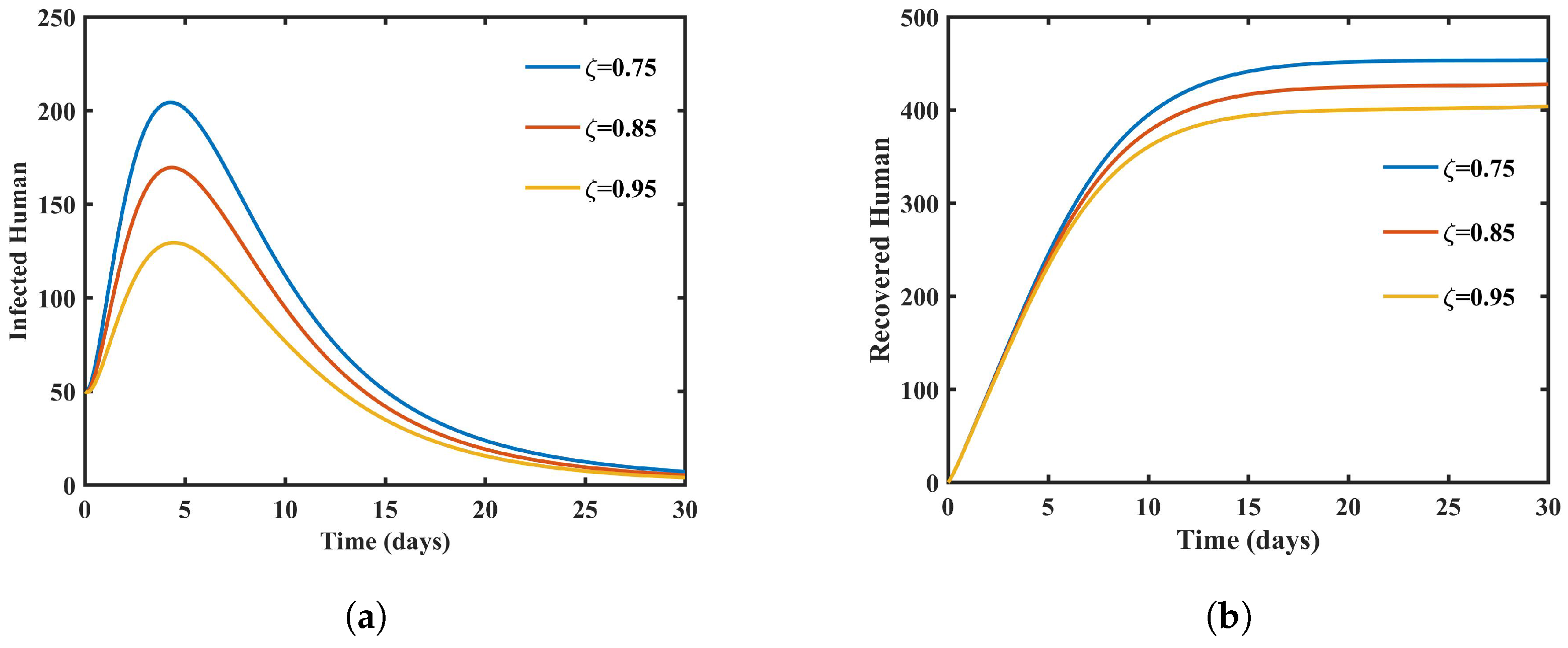
The dynamic correlation between fractional-order variations in populations of dengue patients and those who have recovered from the disease is shown in Figure 2. Interestingly, the number of infected persons decreases significantly as the fractional order increases, suggesting a drop in active dengue virus carriers. This reduction reflects the effectiveness of disease control measures and offers insights into the potential impact of interventions such as vector control, treatment, or vaccination. Conversely, the figure shows a significant increase in the number of recovered individuals with decreasing fractional order, suggesting a faster recovery rate from dengue infection under certain conditions.
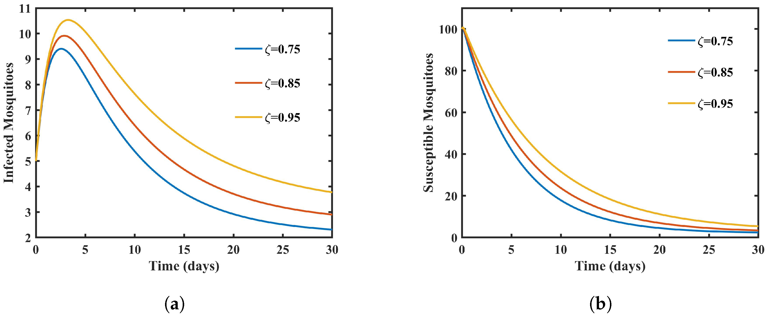
The impact of decreasing the fractional order on vector population dynamics is shown in Figure 3, which primarily highlights the susceptible and infected vector compartments. A key observation is the substantial reduction in the population of susceptible mosquitoes as the fractional order decreases, indicating fewer mosquitoes susceptible to dengue virus infection. This decrease in susceptibility has implications for vector control strategies. Similarly, decreasing the fractional order results in a decrease in the population of infected mosquitoes, reducing the potential transmission of the virus from mosquitoes to humans. These findings underscore the dynamic interplay between fractional-order adjustments and mosquito populations, influencing the overall transmission of dengue.
It is critical for the efficacy of a predictive model to accurately forecast experimental data. We obtained the data of confirmed dengue cases in Makkah, Saudi Arabia, in the year 2017 from [36]. We extracted the data from [36] using the MATLAB function ’GRABIT’. The proposed fractional-order model for dengue infection was validated by comparing its predictions with the actual cases reported in Makkah. We plotted the infected cases predicted by the model and the confirmed cases in Makkah with γ h = 0.288 and ζ = 0.95 , as shown in Figure 4. Successful validation entailed the model closely aligning with the observed data points, indicating that the model captured the underlying dynamics of dengue infection transmission in Makkah. The validation process provided confidence in the model’s ability to accurately predict dengue infection trends in Makkah through rigorous comparison and analysis, thereby supporting its utility for public health planning and intervention strategies.

5. Conclusions

In our comprehensive analysis of the dynamics of dengue transmission using a fractional-order approach, we have identified significant associations between fractional-order changes and the dynamics of susceptible and exposed human populations, infected humans, and mosquito populations. These findings challenge conventional assumptions and provide valuable insights into disease transmission, control, and management. The study focused on investigating the influence of the fractional order on several populations, including susceptible, exposed, infected, and recovered individuals within the human population, as well as susceptible and infected mosquitoes. This counter-intuitive relationship between the fractional order and the population’s vulnerability underscores the complex nature of dengue transmission dynamics. It prompts further investigation into the underlying mechanisms driving these effects and offers a basis for reevaluating disease control strategies.
Building upon these findings, future research in the field of dengue transmission simulation could include the following:
  • Parameter Sensitivity Analysis: A thorough sensitivity analysis could be conducted to identify critical model parameters and their effects on disease dynamics. This will provide valuable insights into the robustness and stability of the model under different conditions.
  • Optimization of Control Measures: To better understand the influence of control techniques on disease transmission and to inform resource allocation for disease management, the model could be used to optimize vaccination campaigns, vector control, and therapeutic interventions.
  • Spatial Considerations: Given that dengue prevalence varies greatly across locations, the model could be extended to consider spatial differences in disease transmission. The integration of spatial dynamics will facilitate the customization of control strategies to particular regions.
  • Climate and Environmental Factors: The effect of the environment and climate on the spread of dengue could be examined, as these conditions are essential to the growth of mosquito vectors.
  • Multi-Pathogen Modeling: In order to investigate possible interactions and co-infections and provide a more complete picture of the disease landscape, other vector-borne illnesses could be included in the model.
In summary, our study contributes to a better understanding of the dynamics of dengue transmission and emphasizes the important influence of fractional-order modifications on the epidemiology of the disease. The future directions outlined above aim to enhance the model’s applicability and its potential to inform evidence-based decision making in dengue control and management.

Author Contributions

Conceptualization, M.Z.M. and A.A.Z.; methodology, S.Z.; software, M.I. and S.Z.; validation, M.I. and M.Z.M.; analysis, A.M.M. and A.A.Z.; investigation, M.I. and A.M.M.; resources, M.I. and M.Z.M.; writing—original draft preparation, S.Z. and M.I.; writing—review and editing, A.A.Z. and A.M.M.; visualization, M.I.; supervision, M.Z.M.; project administration, M.Z.M.; funding acquisition, M.Z.M. All authors have read and agreed to the published final version of the manuscript.

Funding

This research was funded by the Deputyship for Research and Innovation, Ministry of Education in Saudi Arabia ISP-2024.

Data Availability Statement

The original contributions presented in the study are included in the article, further inquiries can be directed to the corresponding author.

Acknowledgments

The authors extend their appreciation to the Deputyship for Research and Innovation, Ministry of Education, Saudi Arabia, for funding this research work under project number ISP-2024.

Conflicts of Interest

The authors declare no conflicts of interest.

References

  1. Bhatt, S.; Gething, P.W.; Brady, O.J.; Messina, J.P.; Farlow, A.W.; Moyes, C.L.; Drake, J.M.; Brownstein, J.S.; Hoen, A.G.; Sankoh, O.; et al. The global distribution and burden of dengue. Nature 2013, 496, 504–507. [Google Scholar] [CrossRef]
  2. Stanaway, J.D.; Shepard, D.S.; Undurraga, E.A.; Halasa, Y.A.; Coffeng, L.E.; Brady, O.J.; Hay, S.I.; Bedi, N.; Bensenor, I.M.; Castañeda-Orjuela, C.A.; et al. The global burden of dengue: An analysis from the Global Burden of Disease Study 2013. Lancet Infect. Dis. 2016, 16, 712–723. [Google Scholar] [CrossRef]
  3. Chan, M.; Johansson, M.A. The incubation periods of dengue viruses. PLoS ONE 2012, 7, e50972. [Google Scholar] [CrossRef]
  4. Carmo, A.M.d.S.; Suzuki, R.B.; Riquena, M.M.; Eterovic, A.; Sperança, M.A. Maintenance of demographic and hematological profiles in a long-lasting dengue fever outbreak: Implications for management. Infect. Dis. Poverty 2016, 5, 7–17. [Google Scholar]
  5. Edussuriya, C.; Deegalla, S.; Gawarammana, I. An accurate mathematical model predicting number of dengue cases in tropics. PLoS Neglected Trop. Dis. 2021, 15, e0009756. [Google Scholar] [CrossRef]
  6. Jain, R.; Sontisirikit, S.; Iamsirithaworn, S.; Prendinger, H. Prediction of dengue outbreaks based on disease surveillance, meteorological and socio-economic data. BMC Infect. Dis. 2019, 19, 272. [Google Scholar] [CrossRef]
  7. Yixin, H.Y.; Carrasco, A.M.; Dong, Y.; Sgrò, C.M.; McGraw, E.A. The effect of temperature on Wolbachia-mediated dengue virus blocking in Aedes aegypti. Am. J. Trop. Med. Hyg. 2016, 94, 812. [Google Scholar]
  8. Ross, P.A.; Axford, J.K.; Yang, Q.; Staunton, K.M.; Ritchie, S.A.; Richardson, K.M.; Hoffmann, A.A. Heatwaves cause fluctuations in w Mel Wolbachia densities and frequencies in Aedes aegypti. PLoS Neglected Trop. Dis. 2020, 14, e0007958. [Google Scholar] [CrossRef]
  9. Brauer, F.; Castillo-Chavez, C.; Feng, Z. Mathematical Models in Epidemiology; Springer: Berlin/Heidelberg, Germany, 2019; Volume 32. [Google Scholar]
  10. Ghori, M.B.; Naik, P.A.; Zu, J.; Eskandari, Z.; Naik, M.U.D. Global dynamics and bifurcation analysis of a fractional-order SEIR epidemic model with saturation incidence rate. Math. Methods Appl. Sci. 2022, 45, 3665–3688. [Google Scholar] [CrossRef]
  11. Fischer, D.B.; Halstead, S. Observations related to pathogenesis of dengue hemorrhagic fever. V. Examination of agspecific sequential infection rates using a mathematical model. Yale J. Biol. Med. 1970, 42, 329. [Google Scholar]
  12. Aguiar, M.; Anam, V.; Blyuss, K.B.; Estadilla, C.D.S.; Guerrero, B.V.; Knopoff, D.; Kooi, B.W.; Srivastav, A.K.; Steindorf, V.; Stollenwerk, N. Mathematical models for dengue fever epidemiology: A 10-year systematic review. Phys. Life Rev. 2022, 40, 65–92. [Google Scholar] [CrossRef] [PubMed]
  13. Dafalla, O.; Abdulhaq, A.A.; Almutairi, H.; Noureldin, E.; Ghzwani, J.; Mashi, O.; Shrwani, K.J.; Hobani, Y.; Sufyani, O.; Ayed, R.; et al. The emergence of an imported variant of dengue virus serotype 2 in the Jazan region, southwestern Saudi Arabia. Trop. Dis. Travel Med. Vaccines 2023, 9, 5. [Google Scholar] [CrossRef]
  14. Zarin, R. Modeling and numerical analysis of fractional order hepatitis B virus model with harmonic mean type incidence rate. Comput. Methods Biomech. Biomed. Eng. 2022, 26, 1018–1033. [Google Scholar] [CrossRef]
  15. Baleanu, D.; Ghanbari, B.; Asad, J.H.; Jajarmi, A.; Pirouz, H.M. Planar system-masses in an equilateral triangle: Numerical study within fractional calculus. Comput. Model. Eng. Sci. 2020, 124, 953–968. [Google Scholar] [CrossRef]
  16. Khan, A.; Zarin, R.; Hussain, G.; Ahmad, N.A.; Mohd, M.H.; Yusuf, A. Stability analysis and optimal control of covid-19 with convex incidence rate in Khyber Pakhtunkhawa (Pakistan). Results Phys. 2021, 20, 103703. [Google Scholar] [CrossRef] [PubMed]
  17. Zarin, R.; Khaliq, H.; Khan, A.; Khan, D.; Akgül, A.; Humphries, U.W. Deterministic and fractional modeling of a computer virus propagation. Results Phys. 2022, 33, 105130. [Google Scholar] [CrossRef]
  18. Jajarmi, A.; Baleanu, D. A new iterative method for the numerical solution of high-order non-linear fractional boundary value problems. Front. Phys. 2020, 8, 220. [Google Scholar] [CrossRef]
  19. Djeddi, K.; Bouali, T.; Msmali, A.H.; Ahmadini, A.A.H.; Koam, A.N. Study Models of COVID-19 in Discrete-Time and Fractional-Order. Fractal Fract. 2023, 7, 446. [Google Scholar] [CrossRef]
  20. Baleanu, D.; Ghassabzade, F.A.; Nieto, J.J.; Jajarmi, A. On a new and generalized fractional model for a real cholera outbreak. Alex. Eng. J. 2022, 61, 9175–9186. [Google Scholar] [CrossRef]
  21. Jajarmi, A.; Baleanu, D.; Vahid, K.Z.; Pirouz, H.M.; Asad, J. A new and general fractional Lagrangian approach: A capacitor microphone case study. Results Phys. 2021, 31, 104950. [Google Scholar] [CrossRef]
  22. Zarin, R.; Khan, A.; Akgül, A.; Akgül, E.K. Fractional modeling of COVID-19 pandemic model with real data from Pakistan under the ABC operator. AIMS Math. 2022, 7, 15939–15964. [Google Scholar] [CrossRef]
  23. Sajjadi, S.S.; Baleanu, D.; Jajarmi, A.; Pirouz, H.M. A new adaptive synchronization and hyperchaos control of a biological snap oscillator. Chaos Solitons Fractals 2020, 138, 109919. [Google Scholar] [CrossRef]
  24. Zarin, R.; Khan, A.; Inc, M.; Humphries, U.W.; Karite, T. Dynamics of five grade leishmania epidemic model using fractional operator with Mittag–Leffler kernel. Chaos Solitons Fractals 2021, 147, 110985. [Google Scholar] [CrossRef]
  25. Haq, F.; Shah, K.; Rahman, G.U.; Shahzad, M. Numerical analysis of fractional order model of HIV-1 infection of CD4+ T-cells. Comput. Methods Differ. Equations 2017, 5, 1–11. [Google Scholar]
  26. Haq, F.; Shah, K.; ur Rahman, G.; Shahzad, M. Numerical solution of fractional order smoking model via Laplace Adomian decomposition method. Alex. Eng. J. 2018, 57, 1061–1069. [Google Scholar] [CrossRef]
  27. ur Rahman, G.; Agarwal, R.P.; Liu, L.; Khan, A. Threshold dynamics and optimal control of an age-structured giving up smoking model. Nonlinear Anal. Real World Appl. 2018, 43, 96–120. [Google Scholar] [CrossRef]
  28. Al-Sulami, H.; El-Shahed, M.; Nieto, J.J.; Shammakh, W. On fractional order dengue epidemic model. Math. Probl. Eng. 2014, 2014, 456537. [Google Scholar] [CrossRef]
  29. Atangana, A. Fractal-fractional differentiation and integration: Connecting fractal calculus and fractional calculus to predict complex system. Chaos Solitons Fractals 2017, 102, 396–406. [Google Scholar] [CrossRef]
  30. Herrmann, R. Fractional Calculus: An Introduction for Physicists; World Scientific: Singapore, 2011. [Google Scholar]
  31. Qureshi, S.; Yusuf, A.; Aziz, S. On the use of Mohand integral transform for solving fractional-order classical Caputo differential equations. J. Appl. Math. Comput. Mech. 2020, 19, 99–109. [Google Scholar] [CrossRef]
  32. Jain, S. Numerical analysis for the fractional diffusion and fractional Buckmaster equation by the two-step Laplace Adam-Bashforth method. Eur. Phys. J. Plus 2018, 133, 19. [Google Scholar] [CrossRef]
  33. Martcheva, M. An Introduction to Mathematical Epidemiology; Springer: Berlin/Heidelberg, Germany, 2015; Volume 61. [Google Scholar]
  34. Slotine, J.J.E.; Li, W. Applied Nonlinear Control; Prentice hall Englewood: Cliffs, NJ, USA, 1991; Volume 199. [Google Scholar]
  35. ul Rehman, A.; Singh, R.; Agarwal, P. Modeling, analysis and prediction of new variants of covid-19 and dengue co-infection on complex network. Chaos Solitons Fractals 2021, 150, 111008. [Google Scholar] [CrossRef] [PubMed]
  36. Melebari, S.; Bakri, R.; Hafiz, A.; Qabbani, F.; Khogeer, A.; Alharthi, I.; Alhazmi, S.; Almalki, Y.; Bulkhi, R.; Gammash, R.; et al. The epidemiology and incidence of dengue in Makkah, Saudi Arabia, during 2017–2019. Saudi Med. J. 2021, 42, 1173. [Google Scholar] [CrossRef] [PubMed]
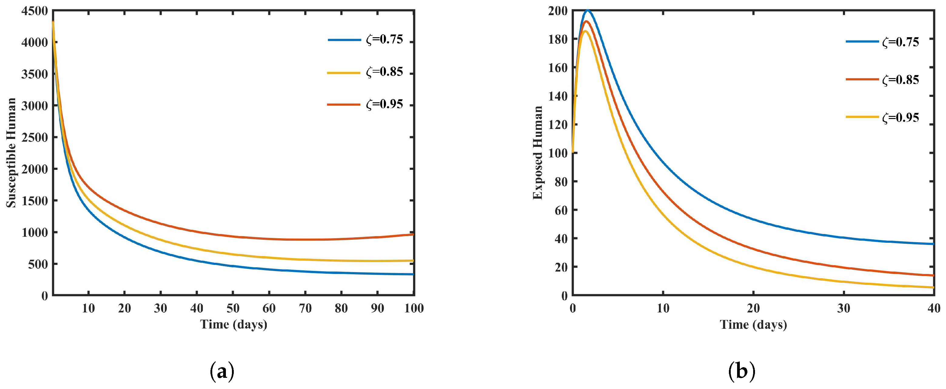
Figure 1. Graphs showing susceptible and exposed humans with different values of ζ . (a) Graph showing susceptible humans with different values of ζ . (b) Graph showing exposed humans with different values of ζ .
Fractalfract 08 00207 g001
Figure 2. Graph showing infected and recovered humans with different values of ζ . (a) Graph showing infected humans with different values of ζ . (b) Graphs showing recovered humans with different values of ζ .
Fractalfract 08 00207 g002
Figure 3. Graphs showing susceptible and infected mosquitoes with different values of ζ . (a) Graph showing susceptible mosquitoes with different values of ζ . (b) Graph showing infected mosquitoes with different values of ζ .
Fractalfract 08 00207 g003
Figure 4. Comparison of infected humans with actual cases reported in Makkah, Saudi Arabia.
Fractalfract 08 00207 g004
Table 1. Description of parameters and their values (see [12] for more details).
SymbolDefinitionValues
Λ h Rate of human recruitment (per day)0.02–0.05
β Parameter (per day)0.7–0.9
d h Death rate of humans0.11–0.26
γ h Incubation rate of humans0.2–0.9
γ v Incubation rate of mosquitoes (per day)0.01–0.06
η Humans who are hospitalized0.002–0.006
δ Disease-related human rate (per day)0.06–0.09
η 1 Recovery rate of infected (per day)0–0.1
q 1 Recovery rate of infected and hospitalized (per day)0–0.06
q 2 Recovery rate of hospitalized (per day)0–0.008
Λ v Recruitment rate of mosquitoes (per day)0.2–0.4
d v Death rate of mosquitoes (per day)0–0.04
Disclaimer/Publisher’s Note: The statements, opinions and data contained in all publications are solely those of the individual author(s) and contributor(s) and not of MDPI and/or the editor(s). MDPI and/or the editor(s) disclaim responsibility for any injury to people or property resulting from any ideas, methods, instructions or products referred to in the content.