1. Introduction
Many real processes are delayed in time, and the resulting memory effects require the use of fractional calculus to model them mathematically. For example, the problems, based on time-fractional derivative and a set of coupled nonlinear ODEs, describes the concentrations of species in so-called compartment problems [
1]. The model posits that each compartment exhibits homogeneity within a well-mixed population. The coupling terms in the ODEs depict interactions among populations in distinct compartments. These terms could entail straightforward constant rate removal processes, or they might signify reactions among various populations. For certain compartmental models, understanding the time of entry of an individual into a compartment is crucial. Fractional-order systems of ODEs are one of the most effective approaches for studying transmission dynamics of epidemic [
2,
3,
4,
5,
6,
7,
8,
9,
10], fractional pharmacokinetic processes [
11], honeybee population dynamics [
12,
13], mechanics [
14], etc. Recently, there has also been an increase in the number of studies based on COVID-19 fractional epidemiological modeling, see e.g., refs. [
15,
16,
17]. One class of these models, describing the spread of an infectious disease, are the SIR (susceptible-infected-removed) compartment model, SEIR (susceptible-exposed-infected-recovered), etc.
A numerical solution of epidemic fractional SIR model of measles with and without demographic effects by using Laplace Adomian decomposition method is presented in [
2]. The effect of the fractional order was investigated. The homotopy analysis method is proposed in [
3] for the SIR model that tracks the temporal dynamics of childhood illness in the face of a preventive vaccine. Authors of [
8] provide some remarkable and helpful properties of the SIR epidemic model with nonlinear incidence and Caputo fractional derivative.
The SEIR fractional differential model with Caputo operator is considered in [
7]. Authors construct a numerical method in order to explain and comprehend influenza A(H1N1) epidemics. They conclude that the nonlinear fractional-order epidemic model is appropriate for the study of influenza and fits the real data.
In [
10], the author proposes a SEIR measles epidemiological model with a Caputo fractional order operator. Existence, uniqueness and positivity of the solution was proved. The problem is solved by the Adams technique. It is shown that the incorporation of memory features into dynamical systems designed for modeling infectious diseases reveals concealed dynamics of the infection that classical derivatives are unable to detect. Existence and uniqueness results for the Caputo fractional nonlinear ODE system, describing transmission dynamics of COVID-19, are obtained in [
15,
17]. In [
13], the author presents a existence, uniqueness and stability analysis for a fractional multi-order honeybee colony population nonlinear ODE system with Caputo and Caputo–Fabrizio operators.
One of the most popular approaches for numerically solving nonlinear ODEs and systems of ODEs with Caputo derivative is the fractional Adam method [
18,
19,
20]. This method is applied, for example in [
10] for solving the Caputo fractional SEIR measles epidemiological problem. In [
17], authors a construct numerical method based on the Adams–Bashforth–Moulton approximation for solving the nonlinear ODEs system with a Caputo operator.
The Newton–Kantorovich method for solving both classical and fractional nonlinear initial-boundary values and initial value problems is employed in many papers, see e.g., refs. [
21,
22,
23,
24]. In [
25], the quasi-Newton’s method, based on the Fréchet derivative, is developed for solving nonlinear fractional order differential equations.
The original concept of the quasilinearization method was developed by Bellman and Kalaba [
26] and recently has been widely investigated and applied by Ben-Romdhane et.al., to several highly nonlinear problems [
27] combined with other methods by Feng et al. [
28] and by Sinha et al. [
29]. By combining the technique of lower and upper solutions with the quasilinearization method and incorporating the Newton–Fourier idea, it becomes possible to simultaneously construct lower and upper bounding sequences that converge quadratically to the solution of the given problem [
30]. This approach, referred to as
generalized quasilinearization, has been further refined and theoretically extended to address a broad class of problems.
The quasilinearization method is a realization of Bellman–Kalaba quasilinearization, representing a generalization of the Newton–Raphson method. It is employed for solving either scalar or systems of nonlinear ordinary differential equations or nonlinear partial differential equations. One can also interpret quasilinearization as Newton’s method for the solution of a nonlinear differential operator equation.
In [
31,
32,
33] existence, uniqueness and convergence results for the generalized quasilinearization method for the Caputo fractional nonlinear differential equation, represented as the Volterra fractional integral equation, are obtained.
Inverse or identification problem solutions have a key role in many practical applications [
34,
35,
36,
37]. It is a process of reconstruction from a set of observations/measurements, unknown parameters/coefficients, and initial conditions or source, i.e., the quantities that cannot be directly measured. Such problems have attracted a lot of attention from many researchers during the last decade. In spite of many results on the existence, uniqueness and stability of the solution for linear ODEs and PDEs, the nonlinearity of the differential equation renders it challenging to solve. In general, inverse problems are highly ill-posed [
34,
35,
36,
37,
38], and this makes them difficult to solve, even numerically. Small fluctuations (noisy measurements) in the input data can lead to significant changes in the outcome. Therefore, to achieve meaningful results, the inversion or reconstruction process requires stabilization, commonly known as regularization.
Numerical methods for solving inverse problems for fractional-order ODEs are proposed in [
14,
39,
40]. The shooting method is employed in [
14] for numerically solving terminal value problems for Caputo fractional differential equations. In [
39], the authors develop a numerical method for recovering a right-hand side function of a nonlinear fractional-order ODE, using Chelyshkov wavelets. Numerical discretizations of inverse problems for Caputo fractional ODEs under interval uncertainty are constructed in [
40].
Recently, a lot of research on inverse problems concern fractional-order nonlinear ODEs systems. In [
41] there is proposed a parameter and initial condition identification block pulse function method for fractional order systems. A time–domain determination inverse problem for fractional-order chaotic systems is solved in [
42] by a hybrid particle swarm optimization–genetic algorithm method. An adaptive recursive least-square method is applied in [
43] for parameter estimation in fractional-order chaotic systems.
In [
44], the authors developed a new numerical approach, based on the Adams–Bashforth–Moulton method, for solving parameter estimation inverse problem for fractional-order nonlinear dynamical biological systems. Time fractional-order biological nonlinear ODE systems in Caputo sense with uncertain parameters are considered in [
4,
5]. In particular, the solution for HIV-I infection and Hepatitis E virus infection models is investigated. In [
45], the author investigate a fractional-order delay nonlinear ODE system to study tuberculosis transmission. A numerical method for recovering dynamic parameters of tuberculosis is developed.
In [
16], authors use the Monte Carlo method based on the genetic algorithm in order to estimate unknown parameters in fractional SIR models, describing the spread of the COVID-19 disease. The authors of [
46] solve the numerical parameter identification inverse problem for the Caputo fractional SIR model, in order to estimate the economic damage of COVID-19 pandemic. They minimize a least-squares cost functional.
The parameter identification inverse problem for the nonlinear ODE system with Caputo differential operator describing honeybee colony collapse was solved numerically in [
12]. The authors applied a gradient optimization method to minimize a quadratic cost functional.
The aim of this paper is to present an extension to the fractional multi-order (
) ODE system, the quasilinearization parameter identification method proposed in [
47,
48] for the classical ODEs system. We develop a robust and convergent numerical method of order
. The approach successfully recovers the unknown parameters even for noisy data. The Tikhonov regularization technique is applied, which increases the range of convergence with respect to the initial guess.
The remaining part of the paper is organized as follows. In the next section, we formulate direct and inverse problems on the base of finite number solution observations. In
Section 3, the fractional-order quasilinearization inverse method is presented. The implementation of the method is described in
Section 4. The usefulness of our approach is illustrated by numerical simulations for SIR and SEIR epidemiological models in
Section 5. The paper is finalized with some conclusions.
2. Direct and Inverse Problems
First, we introduce the direct (forward) problem for the nonlinear fractional differential equation system with initial condition:
where
is a real L-dimensional Euclidean space, and
is the left Caputo fractional derivative of order
for arbitrary function
, i.e.,
y is absolutely continuous on
, and
The vector function
where the symbol ‘;’ stands to underline the dependence on parameter
, is called vector field. We will use also the notation
.
The
direct problem is to determine the solution
, when the parameters
, right-hand side
and initial data
in (
1) are given.
We denote by
the set of functions
which are
n-times differentiable on the interval
endowed by the norm
Here,
is the Euclidean norm when the argument is the vector and the corresponding operator norm if the argument is matrix.
Further, we will suppose that for the vector-valued function,
from (
1) will have continuous partial differential derivatives up to second order
in a bounded convex region
and
We will use the following result of existence and uniqueness of the solution to the problem (
1).
Theorem 1. Let , and the function satisfies the conditions (3) and (4). Then, the problem (1) has one solution , which is the solution of nonlinear Volterra integral equationand vice versa. Proof. For proof, we use the results of [
49], as well of [
19,
50].
The condition (
3) is sufficient for
f to be Lipschitz continuous for all
and
. Also,
,
,
,
. Then, Theorem 2 from [
49] and Theorem 3.1 from [
19] assure global existence of unique solution
to the problem (
1), as well as the representation (
5). □
Further, since the system (
1) depends on the vector parameters
, we state the following assertion.
Corollary 1. Let the conditions of Theorem 1 and (4) be fulfilled. Then, the solution has continuous partial derivatives with respect to .
Proof. Let us consider the auxiliary problem:
Then, the analysis of the system (
6), similar to that of the Theorem 1 provides the proof. □
The inverse problem in this paper consists of identifying the parameter vector
, where
is an admissible set upon the observed behavior of the solution of dynamical system (
1).
The idea of the parameter identification inverse problem is to minimize the difference between a measured state
of the system and the ones calculated with the mathematical model. However, in the real practice, the measurements are available at a final number of times. So, let us denote
,
as the measured state of the dynamical system (
1) and
,
as those obtained by solving the fractional-order differential problem (
1). We gather the residuals for the measurements to be calibrated
in the residual vector
, i.e.
where
means the transpose operation.
We treat the inverse problem in the nonlinear least-square form
This conception is developed in the next section, where a functional of type
with
being residual on iterations of quazilinearization of the problem (
1).
3. Quasilinearization Optimization Approach to (1)
For clarity of the exposition, we describe the method for the simple case of two equations with three unknown parameters, i.e., , .
Let
be an initial approximation. Applying quasilinearization [
26,
51] to (
1), at each iteration
we arrive at the linear Cauchy problem:
Following [
26], for a known parameter vector
, solving the problem (
10) and (
11) one can construct a sequence
, which converges to
with a quadratic rate of convergence. However, we do not know the exact value of parameter
, so that starting from an an initial guess
, after each quasilinearization iteration we specify the parameter value
from the linear system (
10) and (
11) by the following sensitivity scheme.
In line with the theory of sensitivity functions [
52], we present the differences
,
, with second-order accuracy as follows:
The Jacobian
with elements
, called sensitivity matrix,
can be found after solving the system (
10) and (
11). Here,
,
are the corresponding columns of the matrix
.
We suppose the existence of continuous mixed derivatives
,
,
,
. Then, the sensitivity matrix
is a solution of the following matrix equation, obtained by differentiation of the system (
10) with respect to the vector
:
where the Jacobian
is defined as follows
and
is
matrix with elements
The increment
is obtained by minimization of the functional [
47,
48]:
It is easy to see that the functional
is twice continuously differentiable and we have the extremum necessary condition
and
It follows from (
16), that the minimum
satisfies the system of algebraic equations
Therefore,
is
symmetric matrix with elements
and
is a 3-component vector:
The matrix
is a Gram matrix of vectors
and
It is shown in [
47,
48,
53] that
and it is strongly positive, that is to say,
is non-singular if and only if the vectors
,
are linearly independent. In this case, we summarize the approach in the following steps.
Algorithm
Step 1. Choose initial guess , and set .
Step 2. Solve the linear problem (
10) and (
11) to find
, and the system (
14) to find
.
Step 3. Solve the linear algebraic Equations (
17) to find the new parameter value
.
Step 4. One of the expressions can be used as a criterion to stop the iteration process
when it reaches a sufficiently small value. Otherwise,
and go to Step 2.
Now, following results in [
47,
48], more specifically Section 3 in [
47], we discuss the convergence of the quasilinearization method, based on Algorithm for general case
,
.
We suppose that the solution of the problem (
1) satisfies
It follows from (
5), (
10) and (
11) the integral representation
which gives for
:
If we take
, such that
then
. Further, when (
19) holds, by induction follows that
for
.
Also, we suppose that , for sufficiently small and any .
Further, using the representation (
18) and following the line of consideration in (Section 3 of [
47]), we derive
where
and
.
Additionally, as in [
47], one can deduce for the functional
,
of (
12), the inequalities
If we require , then there exists a limit .
Furthermore, if the functional
is a strong convex function with convex constant
, see [
54], then, following the results of Section 3 in [
47], one can show that
and
Therefore, the next assertion holds.
Theorem 2. Assume that the vector-function and its second-order derivatives (3) and (4) are continuous and bounded as . Let , be solution to the problem (1) and assume that the conditions (20)–(22) are fulfilled. Then, the Algorithm for the general case , is convergent with quadratic rate of convergence and the estimate (23) holds. 5. Numerical Simulations
In this section, we illustrate the efficiency of the developed method for recovering three and four parameters in biological ODE systems with two and four equations, respectively. We give absolute (
) and relative (
), errors of the recovered parameters
and relative errors (
,
) of the solution in maximal and
norms, respectively
for different fractional orders
. Here,
,
is the exact (true) value of the parameter
,
and
are the recovered parameter and solution at time layer
, and
is the reference solution of the ODEs system at time layer
, which can be the exact or numerical solution of the direct problem with exact values of the parameters, i.e.,
.
In addition, we perform simulations to illustrate the model behavior with respect to parameters.
We will also investigate the case of noisy measurements, generated by
where the measurements
are obtained from direct problem,
is the noise level, and
is an
M-dimensional random variable with standard normal distribution.
We take
, and the computations are conducted mainly for the more intricate scenario of a weak singular solution in graded mesh (
29).
5.1. System of Two Equations with Three Unknown Parameters
First, we consider a simplified prototype of SIS fractional order epidemic model [
2,
5,
8], describing the dynamics of susceptible
and infectious
individuals at any time
t Typically in such models
,
,
and
are constants, representing transmission, birth, death and recovery rates, respectively.
The inverse problem is formulated for recovering the parameters , and computations are performed by Algorithm 1 with . We assume that and the measurements are performed at grid nodes.
Example 1.
(Direct problem). First, we test the accuracy of the numerical discretization (24) and (25) for solving the direct problem (31), in the case of weak singular solution. To this aim, we add residual functions and in the right-hand side of the differential equations in (31), such that the exact solution is to be , , where , is the Mittag–Leffler function, namely . That corresponding to the (
24) and (
25) discretization for the modified system (
31) with an exact solution is
where
and
.
We compute the solution of the direct problem from (
32), initiating iteration process at each time layer with stopping criteria
, for exact values of the parameters
and
[
3].
Note that in inverse problem Algorithms 1 and 2, to find the solution , an iterative process with the same termination criteria is used to find the solution .
In
Table 1 we present errors and the corresponding orders of convergence
for different and equal orders of the fractional derivative. We observe that the accuracy of the solutions
S is
and that of the solution
I is
, both in maximal and
norms. Therefore, the convergence of the numerical solution of the system (
31) is
, where
or
.
Example 2.
(Inverse problem: exact measurements). We consider an inverse problem for recovering parameters in the ODE system (31) with an exact solution, modified just as in Example 1. We consider noisy-free data (), and the measurements in (30) are equal to the numerical solution of the direct problem, computed by (24) and (25) for the true values . The sensitivity problem (26) is where , , , , . The regularization parameter is determined experimentally, by multiple runs, such that to avoid singularity of the matrix
(very small
) and to obtain convergent iteration process. In
Table 2, we give the regularization parameter, recovered values of
, errors of the recovered values of the parameters and solution, and number of iterations
k for different initial guesses
and fractional orders,
,
. The reference value of the recovered solution
is the exact solutions
. Results show that independently of the fractional order, the recovering of the parameters is almost exact, and the accuracy of the restored solution
is similar to the accuracy of the discrete solution of the direct problem. Therefore, we conclude that the order of convergence of the numerical method for solving PIIP with noisy-free data has the same order of convergence as the numerical method of the direct problem.
For comparison, we give also the results for integer order derivative. In this case, L1 approximation is replaced by forward time stepping. We observe that the recovering of the parameters is with higher precision, and the obtained values of the solution have the same accuracy as the discrete solution of the direct problem. Note that for this example, regularization is not required.
The convergence of the method without regularization is limited in relation to the size of the convergence range for the initial guess . Moreover, for this test example, a smaller leads to a bigger singularity of , and convergence is achieved in more iterations. Nevertheless, applying the regularization approach, the parameters are successfully recovered. It is not a surprise that, if the initial guess approaches the true values , the regularization parameter can be decreased, the iteration process requires smaller number of iterations, and the accuracy improves.
For completeness, we illustrate the performance of the numerical approach for the smooth solution in the sense of Theorem 1. We repeat the same experiment as in
Table 2, but now, we take the exact solution to be
,
, and the mesh is uniform. The computational results are listed in
Table 3. The parameter recovering is more accurate than the case of weak singular solution, and for most sets of initial guesses, the convergence is attained for a smaller number of iterations. Furthermore, in most cases, except for
,
and initial guess
, the recovering without regularization fails.
Computational results in this example showed that if the system is not ill-conditioned, and thus if the regularization is not used, the recovering of the parameters is almost exact. Otherwise, the use of regularization is strongly recommended in order to obtain a convergent iteration process, although this is at the expense of the accuracy of the restored parameters. Nevertheless, the recovery is with good enough precision such that the reconstructed solution is with optimal accuracy.
Further, all experiments are performed for the case of weak singular solution.
Example 3.
(Inverse problem: noisy measurements). The test’s problem is the same as in Example 2, but now, we add a noise, i.e., and in (30). We consider three levels of noise: (, ), (, ) and (, ). The computations are performed for
,
and different fractional orders. In the case of
, we take
, while for
,
, we set
. In
Table 4 we give the numerical results. The noise level has a bigger impact on the precision of the recovered parameters in the case of derivatives with different fractional orders of large range than the case of moderate and equal values of the fractional orders, but the convergence is faster. For
, the iteration process requires twice as many iterations than for the case of
,
. In both scenarios, the precision of the determined parameters is optimal, such that the solution
is sufficiently accurate.
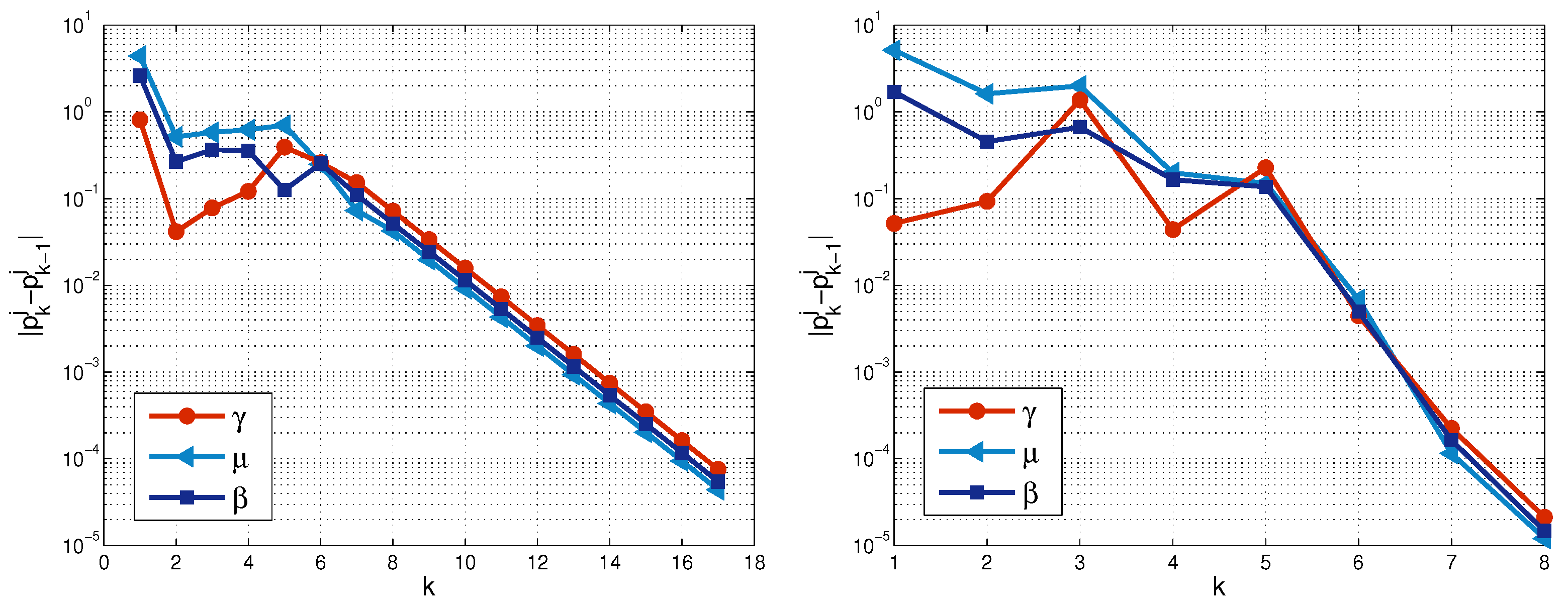
In
Figure 1, we illustrate the convergence of the iteration process, namely, we represent the values of
at each iteration for
and
,
and
noise. For both set of parameters, we observe the fluctuation at initial iterations, and then, as was mentioned above, for
, the convergence is attained at a small number of iterations compared to the case
,
. We believe that the reason is in the smaller regularization parameter and bigger grading of the mesh, which is prescribed by (
29).
5.2. System of Four Equations with Four Unknown Parameters
We consider the following dynamical system SEIR model, describing measles epidemic [
10].
where
,
,
,
are susceptible, exposed, infectious and the recovered individuals at time
t, measured in months. The epidemiological model parameters describe recruitment rate
, transmission coefficient rate
, natural death rate
, rate of exposure to the epidemic
and recovery rate
. Let the total population be
. If the birth
rate is equal to death rate
, then
N is a constant, and the problem (
33) reduces to a system or three equations. Namely, the function
is determined from algebraic relation of the total population conservation.
For the simulations, we use the data from [
10] for real confirmed measles incidence cases for May–December, 2018 in Pakistan
incorporated in the normalized model (
33).
The inverse problem is to recover the vector
. We use the numerical solution of the direct problem (
33) and (
34), as a reference (exact) solution and as the measured solution
in (
30).
The computations are performed for the system (
33) and (
34), involving rescalling
,
,
,
and to reduce the computational time, we use also the transformation
.
The additional challenging in this example is that we need to recover parameters with a very different order of magnitude. We apply both Algorithms 1 and 2 for more general case and .
Example 4.
(Inverse problem: noisy measurements at each ). We compute the solution of the inverse problem for noisy data (30), , , , , measured at each grid node (). The final time is months and . The level of the noise of is illustrated on Figure 2. We consider two choices of the initial guess and and examine the performance of Algorithms 1 and 2.
Vector
is chosen by giving one and the same deviation of each element of
. The values of this deviation in percentages are given in
Table 5. Errors of the recovered parameters
and solution
for different regularization are presented in
Table 5, as well.
We observe that the proposed numerical identification algorithm, realized by both algorithms, recovers the unknown parameters and solution
with optimal accuracy. As can be expected, the regularization (
28) is successful even for initial guess that differs significantly from their true values. The iteration process converges in four to five iterations.
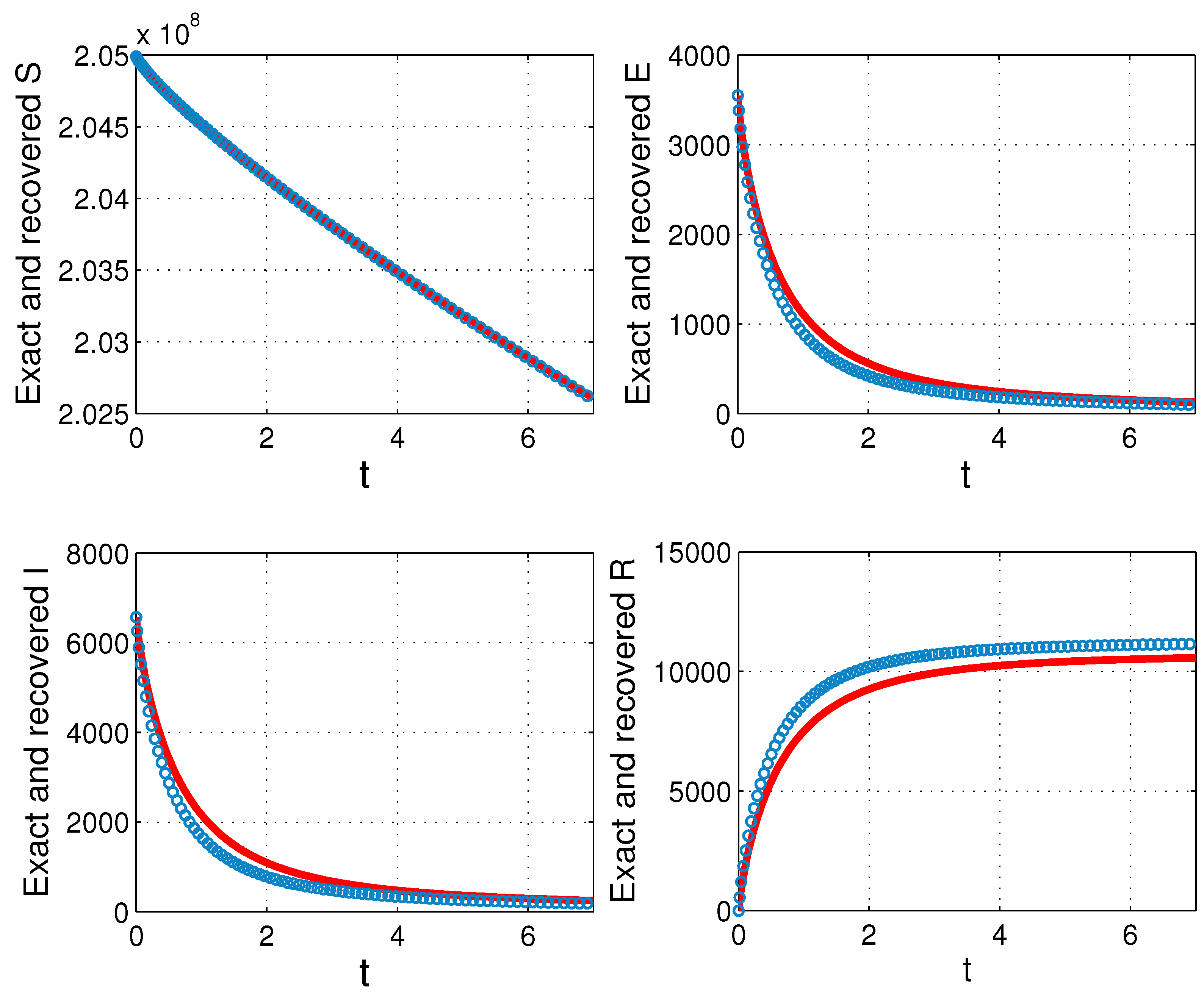
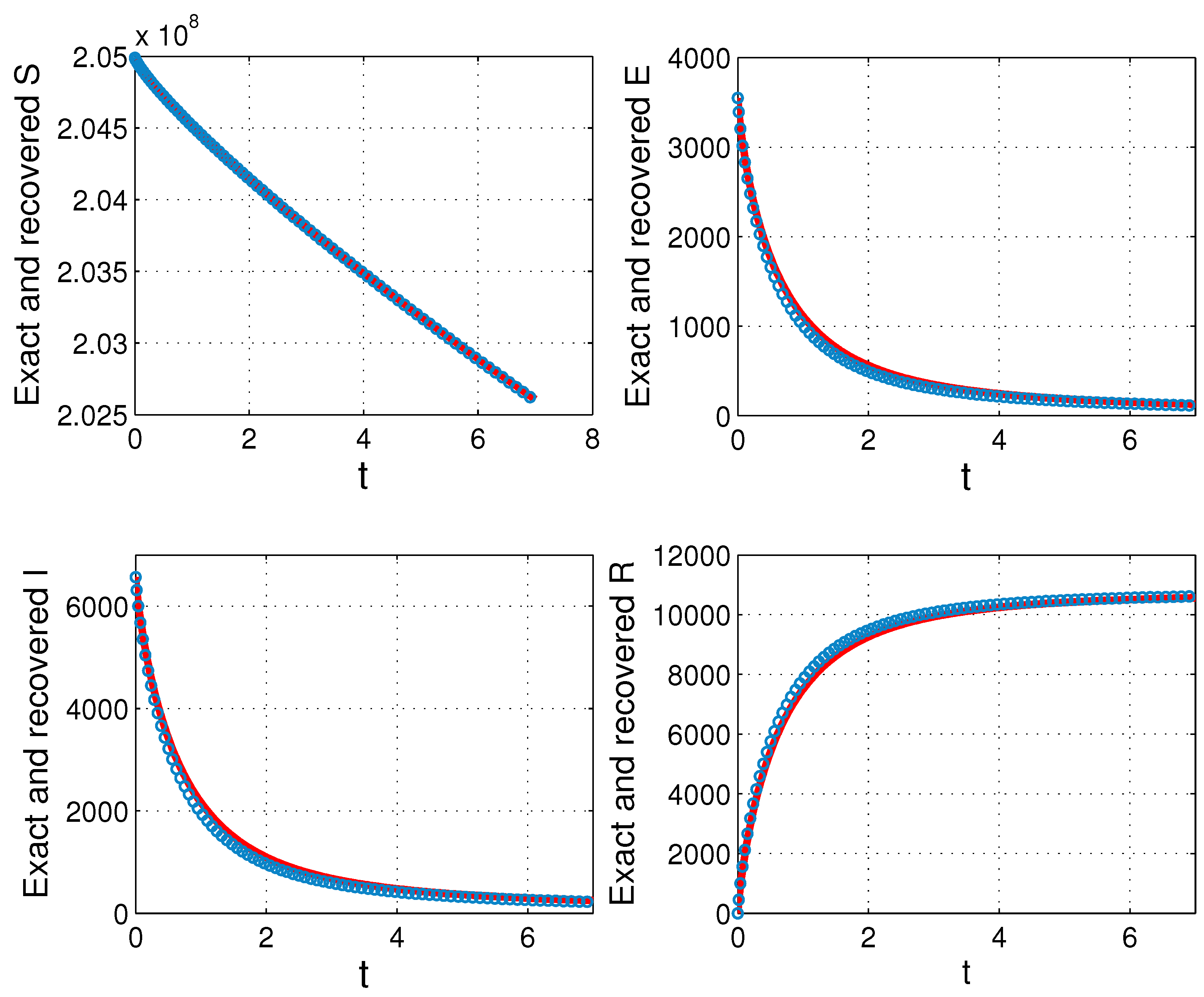
In
Figure 3 and
Figure 4, we depict an exact and recovered solution of the system (
33) for initial guess
and
, computed by Algorithms 1 and 2, respectively. The better fitting of the recovered solution to the exact one is attained by Algorithm 2.
Example 5.
(Inverse problem: noisy measurements at grid nodes). We repeat the experiments from Example 4 with only difference that now, we take measurements at grid nodes. The observations are generated from numerical solution of the direct problem at nodes, giving the same noise levels as in Example 4. Then, we generate simulated measurements interpolating data on the time mesh. The results are listed in Table 6. We establish that the values of the recovered parameters and corresponding errors are very closed to the ones in Table 5. 


