Article

Adaptive Terminal Sliding-Mode Synchronization Control with Chattering Elimination for a Fractional-Order Chaotic System

School of Mathematics and Statistics, Xiamen University of Technology, Xiamen 361024, China
Fractal Fract. 2024, 8(4), 188; https://doi.org/10.3390/fractalfract8040188
Submission received: 14 January 2024 / Revised: 13 March 2024 / Accepted: 20 March 2024 / Published: 25 March 2024
(This article belongs to the Special Issue Robust and Adaptive Control of Fractional-Order Systems, 2nd Edition)

Abstract

:
In this paper, an adaptive terminal sliding-mode control (ATSMC) method is proposed for the synchronization of uncertain fractional-order chaotic systems with disturbances. According to the sliding-mode control theory, a non-singular sliding surface is constructed. To overcome the chattering problem of ATSMC, a smooth term is used in the controller. In order to reduce the estimation error of an uncertain parameter, adaptive laws are designed to adjust the amplitude of the continuous function. Based on the Lyapunov stability theory, a stability analysis of the error system is performed to ensure that the tracking error eventually converges to the origin. The effectiveness and applicability of the proposed control strategy are verified using the simulation results.

1. Introduction

Chaos refers to the state trajectory of a deterministic nonlinear system, which appears as a seemingly random chaotic motion. Because of its random, aperiodic, ergodic and sensitive dependence on initial values, it often appears in mathematical models and engineering applications with physical significance [1,2,3]. In addition to appearing in nature (such as atmospheric turbulence), chaos can also be observed in many natural disciplines (such as nonlinear dynamics) [4]. A chaotic system is one whose long-term behavior is sensitive to the initial conditions. When the initial conditions change slightly, the response of a chaotic system may change completely [5]. Therefore, the study of chaos has also transitioned from trying to describe and understand chaotic phenomena to trying to control chaos. So far, chaos synchronization has become a focus because of its unique advantages in signal processing, secure communication and other expression fields, and many methods have been proposed, for instance, linear matrix inequality [6,7], backstepping control [8,9,10], power integral control [11,12], non-fragile control [13], etc. These methods have injected new vitality into the development and perfection of chaos control and synchronization theory.
On the other hand, fractional calculus and integral calculus have almost the same history. Fractional calculus is an extension of integral calculus in any order, and its dynamic characteristics not only inherit the characteristics of integral calculus, but also increase the characteristics of historical memory, inheritance and the wider parameter adjustment range. With the development of science and technology, fractional calculus has been applied to practical engineering in recent years. Fractional calculus is more accurate than integral calculus in describing the physical phenomena in engineering applications and more in line with engineering practice. Thus, fractional calculus has high research value in electronic circuits [14,15], electromagnetic waves [16,17], secure communication [18,19], image encryption [20] and other fields. Through the in-depth study of chaos, scholars have found that fractional calculus is an effective theory for the analysis and explanation of chaos. Fractional-order chaotic systems (FOCSs) have become a research hotspot, and compared with integer order, FOCSs have more complex dynamic behavior and higher degrees of freedom. Many scholars have conducted extensive research on FOCSs and their synchronization control, such as observer-based approaches [21,22], optimal control [23], impulse control [24,25], etc. It should be emphasized that in the above literature, the design of the controller requires prior knowledge of the system model.
As is well know, in the modeling process of a real system, there are usually some differences between the controlled object and its mathematical model, which can be reflected in the external disturbance, unmodeled dynamics and parameter variation [26,27]. For the synchronization of uncertain FOCSs, sliding-mode control (SMC) is a common and effective method, which originates from variable-structure control systems and is robust to uncertainty and disturbance [28]. In [29], a terminal SMC was used to synchronize FOCSs with parameter uncertainty. In [30], for the synchronization of FOCSs, a fractional-order SMC was designed. In [31], an SMC scheme using only the output information was designed to achieve the synchronization of FOCSs with disturbance. In [32], the synchronization of two uncertain FOCSs was studied by establishing an adaptive SMC scheme. In [33], an adaptive SMC was used to analyze FOCSs with external bounded disturbances and uncertainties. However, in the above literature, the chattering phenomenon is obvious. Therefore, methods to effectively solve this problem are worth studying further.
The chattering problem caused by the existence of discontinuous functions in traditional SMC prevents its wide application. Therefore, determining how to compensate for the defects of SMC to improve the performance of FOCSs is always an important problem in control engineering and control science. In [34], a proposed non-singular SMC method effectively reduced the chattering phenomenon. In [35], an adaptive SMC based on a fractional-order observer was used to reduce the chattering phenomenon of FOCSs’ synchronization with unknown disturbance. In [36], an improved adaptive SMC was proposed to synchronize FOCSs with completely unknown parameters. In [37], an SMC method based on a proportional integral derivative was proposed to realize the synchronization of FOCSs with uncertainties. In [38], an improved sliding surface was proposed to reduce the chattering of FOCSs. However, in the above literature, only asymptotic stability can be guaranteed, i.e., the convergence time may be very long. Therefore, improving the convergence speed is a very important goal.
Inspired by the above discussion, an adaptive terminal sliding-mode control (ATSMC) strategy is proposed for uncertain FOCS synchronization with disturbances. The main contributions are as follows. (1) A new sliding surface is designed, which can effectively reduce the chattering phenomenon. (2) For uncertain FOCSs with disturbances, an ATSMC scheme is proposed to ensure a synchronization control effect, which can significantly reduce the chattering phenomenon and improve the convergence speed simultaneously.
The remainder of this paper is arranged as follows. In Section 2, some basic knowledge of the fractional calculus and descriptions of uncertain FOCSs with disturbances are presented. Section 3 expresses a new fractional-order non-singular sliding face, an adaptive terminal sliding-mode synchronization controller, adaptive laws and Lyapunov stability analysis. In Section 4, the simulation results are provided. Section 5 is the conclusion of this paper. Moreover,  R Γ ( · )  and  R n  denote the real number space, the Gamma function and the n-dimensional vector space, respectively.  x 1  represents the first norm of an n-dimensional vector x, which is defined by  | | x | | 1 = i = 1 n | x i | . For convenience, the variable t is omitted if it does not cause ambiguity. For convenience, all the abbreviated terms and symbols in this paper are shown in Table 1.

2. Preliminaries and System Description

2.1. Fractional Calculus

In this subsection, some necessary knowledge of fractional calculus is presented to facilitate the subsequent analysis.
Definition 1
([39]). The α-order fractional integral is defined as
I t α f ( t ) = 1 Γ ( α ) 0 t f ( τ ) ( t τ ) 1 α d τ ,
with  0 < α < 1 .
If there is no special designation,  i = 1 , 2 , , n , and only an order case of the FOCS that lies in (0, 1) is considered.
Definition 2
([39]). The Caputo fractional derivative is defined as
D t α f ( t ) = 1 Γ ( 1 α ) 0 t f ( υ ) ( t υ ) α d υ .
Definition 3
([39]). The Riemann–Liouville fractional derivative is
D t α f ( t ) R L = 1 Γ ( 1 α ) d d t 0 t f ( υ ) ( t υ ) α d υ .
For convenience,  D t α  and  D t α R L  are used to represent the Caputo and Riemann–Liouville fractional derivatives, respectively. For fractional calculus, there exists the following conclusion.
Lemma 1
([40]). Let f be a continuously differentiable function. Then, it holds that
D t α f T f 2 f T D α f .

2.2. Descriptions of the FOCSs

In this article, two uncertain FOCSs are considered as primary–secondary systems. Let the primary system be
D t α y i = f i ( y ) + f i ( y ) + d i f ( t ) ,
and the secondary system be
D t α x i = g i ( x ) + g i ( x ) + d i g ( t ) + u i ( t ) ,
where  α  signifies the system’s order;  f i ( · )  and  g i ( · ) R  are known nonlinear functions;  y = [ y 1 , y 2 , , y n ] T x = [ x 1 , x 2 , , x n ] T R n  demonstrate the states of the primary–secondary system, respectively;  f i ( · ) g i ( · ) d i f ( · ) d i g ( · ) R  represent the unknown uncertainties and disturbances of the primary–secondary system; and  u i ( · ) R  denotes the control input.
The synchronization error is defined as  e ( t ) = [ e 1 , e 2 , , e n ] T = y x . The main control objective of this paper is to synchronize fractional-order primary and secondary chaotic systems (4) and (5) in a finite time.
Assumption 1.
The uncertainties  f i ( y )  and  g i ( x )  are bounded, i.e., there are suitable and unknown constants  γ i f > 0 γ i g > 0  and  γ i > 0  satisfying
| f i ( y ) | γ i f , | g i ( x ) | γ i g ,
| f i ( y ) g i ( x ) | γ i .
Assumption 2.
The disturbances  d i f ( t )  and  d i g ( t )  are bounded, i.e., there are suitable and unknown constants  δ i f > 0 δ i g > 0  and  δ i > 0  satisfying
| d i f ( t ) | δ i f , | d i g ( t ) | δ i g ,
| d i f ( t ) d i g ( t ) | δ i .
By subtracting (5) from (4), the synchronization error can be rewritten as
D t α e i = f i ( y ) + f i ( y ) + d i f ( t ) g i ( x ) g i ( x ) d i g ( t ) u i ( t ) .
In order to ensure that the error system (10) can converge to an equilibrium in a finite time, a fractional-order ATSMC scheme is proposed below.

3. Main Results

In this article, a fractional-order non-singular sliding surface is designed to synchronize the primary–secondary system, which can be divided into two stages. In the first stage, the system state can reach the sliding surface from any initial position. In the second phase, the system moves along the sliding surface to an equilibrium point under the action of the control input.
Let the sliding surface be
s i ( t ) = D t α 1 e i + D t α 2 ( λ i e i + λ i | e i | ν tanh e i ) ,
where  s = [ s 1 , s 2 , , s n ] T R n ν ( 0 , 1 )  is a constant and  λ i  is a positive parameter of the sliding surface. Then, it holds that
s ˙ i ( t ) = D t α e i + D t α 1 ( λ i e i + λ i | e i | ν tanh e i ) .
According to the sliding conditions  s ˙ i = 0  and  s i = 0 , one obtains
D t α e i = D t α 1 ( λ i e i + λ i | e i | ν tanh e i ) .
Note that multiplying  D t 1 α R L  on both sides of (13) results in  e ˙ i = ( λ i e i + λ i | e i | ν tanh e i ) , which is the same as the general sliding surface form. In addition, the parameters in Equations (12) and (13) need to be satisfied with  ν ( 0 , 1 )  and  λ i > 0 . In order to facilitate the achievement of the control goal, one needs the following lemmas.
Lemma 2.
For any  x R  and  y > 0 , it holds that
s i g n ( x ) tanh y x 0 .
Proof. 
According to the hyperbolic tangent function definition, one obtains
s i g n ( x ) tanh y x = s i g n ( x ) e y x e y x e y x + e y x .
If we multiply the numerator and denominator of the above formula by  e y x , it holds that
s i g n ( x ) tanh y x = 1 e 2 y x + 1 s i g n ( x ) ( e 2 y x 1 ) .
It is clear that
1 e 2 y x + 1 > 0 , s i g n ( x ) > 0 , e 2 y x 1 > 0 , f o r x > 0 s i g n ( x ) 0 , e 2 y x 1 0 , f o r x 0 .
Then, one obtains
s i g n ( x ) tanh y x = 1 e 2 y x + 1 s i g n ( x ) ( e 2 y x 1 ) = s i g n ( x ) e y x e y x e y x + e y x 0 .
This completes the proof. □
Remark 1.
It should be emphasized that in Lemma 2,  x tanh y x 0  also holds. Under predetermined conditions, x and  tanh y x  will be the same sign, so Lemma 2 also yields  x tanh y x 0 , which can be seen in [41].
Lemma 3
([42]). For the sliding surface (11), the error state (10) with zero initial conditions can converge to the origin  e ( t ) = 0  in a finite time.
Proof. 
The Lyapunov candidate function is determined as follows:
V e ( t ) = e ( t ) 1 .
Then, it holds that
V e ˙ ( t ) = i = 1 n s i g n ( e i ) e ˙ i = i = 1 n s i g n ( e i ) R L D t 1 α ( D t α e i ) .
Upon introducing (13) into (20), one obtains
V e ˙ ( t ) = i = 1 n s i g n ( e i ) e ˙ i = i = 1 n s i g n ( e i ) R L D t 1 α ( D t α 1 ( λ i e i + λ i | e i | ν tanh e i ) ) = i = 1 n λ i | e i | + λ i | e i | ν s i g n ( e i ) tanh e i i = 1 n λ i | e i | + λ i | e i | ϵ χ i = 1 n | e i | + i = 1 n | e i | ϵ = χ e ( t ) 1 + e ( t ) 1 ϵ = χ V e ( t ) χ V e ϵ ( t ) ,
where  | e i | ϵ < | e i | ν s i g n ( e i ) tanh e i χ = min 1 i n λ i  and  ϵ  is a constant. In (21), the error state  e i  can converge to the origin. The calculations of the settling time  t s  ( e i  to reach the origin) are given. According to [29] (Lemma 3), from the settling time  t r  ( e i  to reach the sliding surface) to the reaching time  t s , one obtains
t s 1 χ ( 1 ϵ ) ln e ( t r ) 1 1 ϵ + 1 + t r .
This completes the proof. □
Remark 2.
It should be noted that  t r  is finite in (22), and the relevant proof (33) is shown below.
Next, according to (10), the controller  u i ( t )  is constructed as follows:
u i ( t ) = f i ( y ) g i ( x ) + D t α 1 ( λ i e i + λ i | e i | ν tanh e i ) + ζ i tanh μ i s i + γ ^ i tanh s i + δ ^ i tanh s i + M i | s i | κ tanh s i + N i s i ,
with the adaptation laws
γ ^ ˙ i = η i | s i | , δ ^ ˙ i = η i | s i | , ζ ˙ i = p i | s i | | e i | , μ ˙ i = q i | s i | | e i | ,
where  ζ i > 0  and  μ i > 0  are adaptive parameters that regulate the amplitude of the hyperbolic tangent function, and  γ ^ i > γ i | tanh s i | δ ^ i > δ i | tanh s i | κ ( 0 , 1 ) M i N i p i  and  q i  are positive constants.
Based on (11), (23) and (24), this paper has the following results.
Theorem 1.
For the synchronization error system (10), if the controller (23) and adaptive laws (24) are adopted, then the trajectories of the synchronization error can converge to the sliding surface  s ( t ) = 0  in a finite time.
Proof. 
The positive definite Lyapunov candidate function is determined as follows:
V s ( t ) = s ( t ) 1 .
Then, it holds that
V ˙ s ( t ) = i = 1 n s i g n ( s i ) s ˙ i ( t ) .
Substituting (12) into (26), it holds that
V ˙ s ( t ) = i = 1 n s i g n ( s i ) D t α e i + D t α 1 ( λ i e i + λ i | e i | ν tanh e i ) .
Introducing (10) into (27), one obtains
V ˙ s ( t ) = i = 1 n s i g n ( s i ) [ f i ( y ) + f i ( y ) + d i f ( t ) g i ( x ) g i ( x ) d i g ( t ) u i ( t ) + D t α 1 ( λ i e i + λ i | e i | ν tanh e i ) ] .
Using (23) in (28) and simplifying (28), one obtains
V ˙ s ( t ) = i = 1 n s i g n ( s i ) [ f i ( y ) + d i f ( t ) g i ( x ) d i g ( t ) ζ i tanh μ i s i γ ^ i tanh s i δ ^ i tanh s i M i | s i | κ tanh s i N i s i ] .
According to Assumptions 1–2, one has
s i g n ( s i ) [ f i ( y ) g i ( x ) ] | f i ( y ) g i ( x ) | γ i
and
s i g n ( s i ) [ d i f ( t ) d i g ( t ) ] | d i f ( t ) d i g ( t ) | δ i .
From  γ ^ i > γ i | tanh s i |  and  δ ^ i > δ i | tanh s i | , one obtains  γ ^ i s i g n ( s i ) tanh s i > γ i  and  δ ^ i s i g n ( s i ) tanh s i > δ i .
Thus, combining Lemma 2 and simplifying (29), one obtains
V ˙ s ( t ) = i = 1 n s i g n ( s i ) [ f i ( y ) g i ( x ) ] + i = 1 n s i g n ( s i ) [ d i f ( t ) d i g ( t ) ] i = 1 n γ ^ i s i g n ( s i ) tanh s i i = 1 n δ ^ i s i g n ( s i ) tanh s i + i = 1 n s i g n ( s i ) [ ζ i tanh μ i s i M i | s i | κ tanh s i N i s i ] i = 1 n ζ i s i g n ( s i ) tanh μ i s i + M i | s i | κ s i g n ( s i ) tanh s i + N i | s i | i = 1 n M i | s i | κ s i g n ( s i ) tanh s i + N i | s i | ξ i = 1 n | s i | h + | s i | = ξ s ( t ) 1 + s ( t ) 1 h = ξ V s ( t ) ξ V s h ( t ) ,
where  | s i | h < | s i | κ s i g n ( e i ) tanh e i ξ = min 1 i n [ M i , N i ]  and h is a constant. According to (32), the error state  e i  can converge to the sliding surface  s ( t ) = 0 . In [29] (Lemma 3), from 0 to the reaching time  t r , the calculation of the reaching time  t r  is given, and one obtains
t r 1 ξ ( 1 h ) ln s ( 0 ) 1 1 h + 1 .
This completes the proof. □
Remark 3.
In order to eliminate chattering, this paper tries to use the adaptive  t a n h ( · )  instead of the  s i g n ( · ) . In theory, the steeper the gradient of  t a n h ( · ) , the closer the result is to the  s i g n ( · ) . Thus, the magnitude of the error is determined by the steepness of the  t a n h ( · ) . On this basis, a  t a n h ( · )  with sufficient steepness is designed as a  s i g n ( · )  to try to eliminate the impact caused by chattering. On the other hand, the degree of chattering is positively correlated with the gain of  s i g n ( · )  [43]. Therefore, this paper eliminates chattering and maintains the presence of the sliding surface by reducing the steepness of the  t a n h ( · ) . In this paper,  ζ i  and  μ i  are responsible for regulating the amplitude of  t a n h ( · ) .
Remark 4.
According to Theorem 1, the convergence time can be reduced by adjusting the values of  λ i , ν, κ,  M i  and  N i . Moreover, the smooth terms included in the designed sliding surface and synchronization controller help the FOCS reach the sliding surface faster. In addition, the terms  | e i | ν tanh e i  and  | s i | κ tanh s i  can enhance the convergence of approaching equilibrium. Therefore, compared with other sliding surfaces, the sliding surface (11) can achieve finite-time convergence faster.

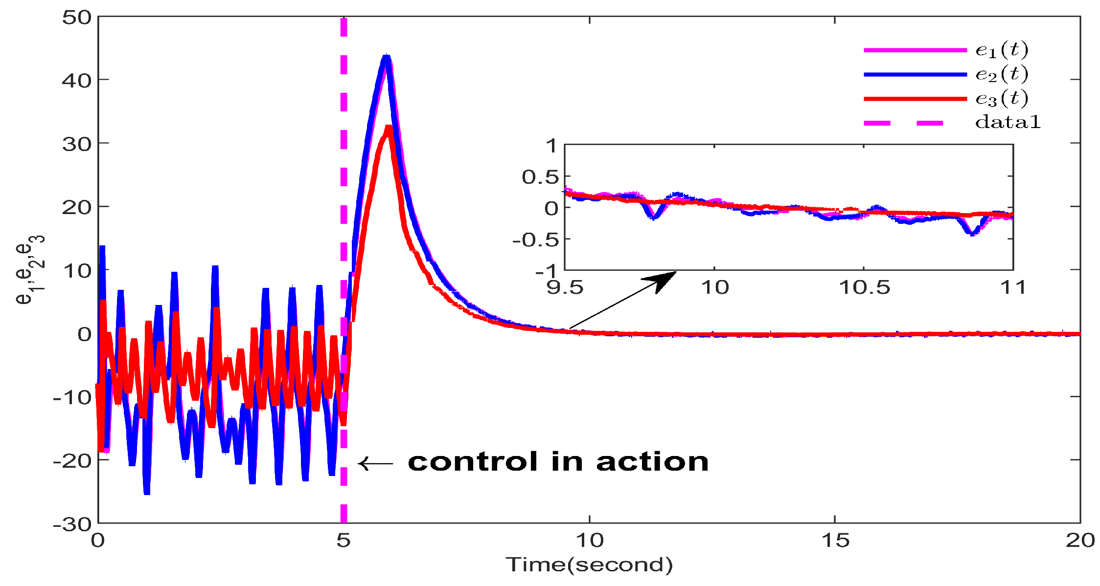
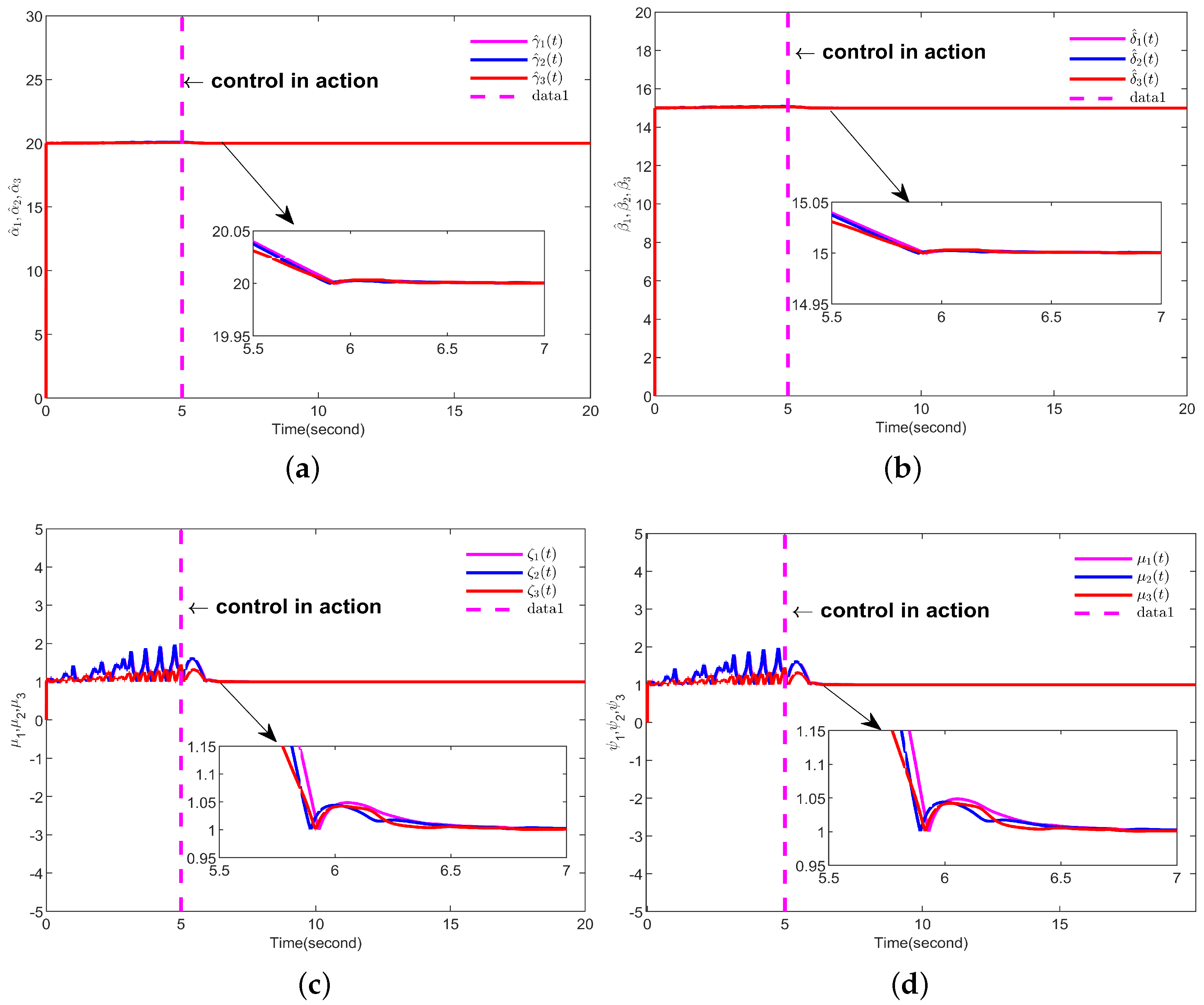
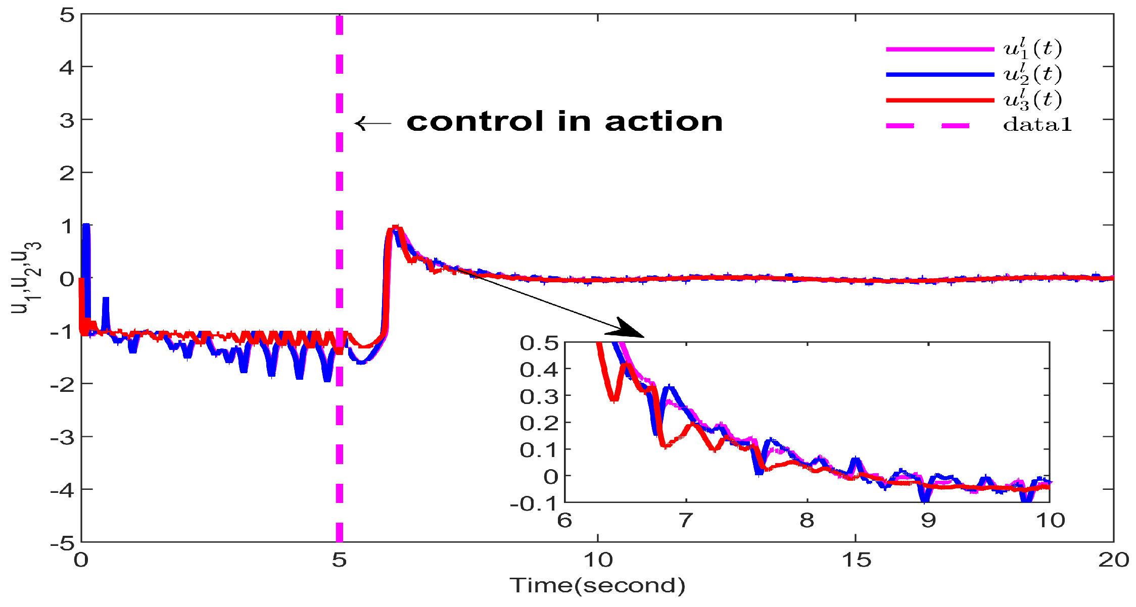
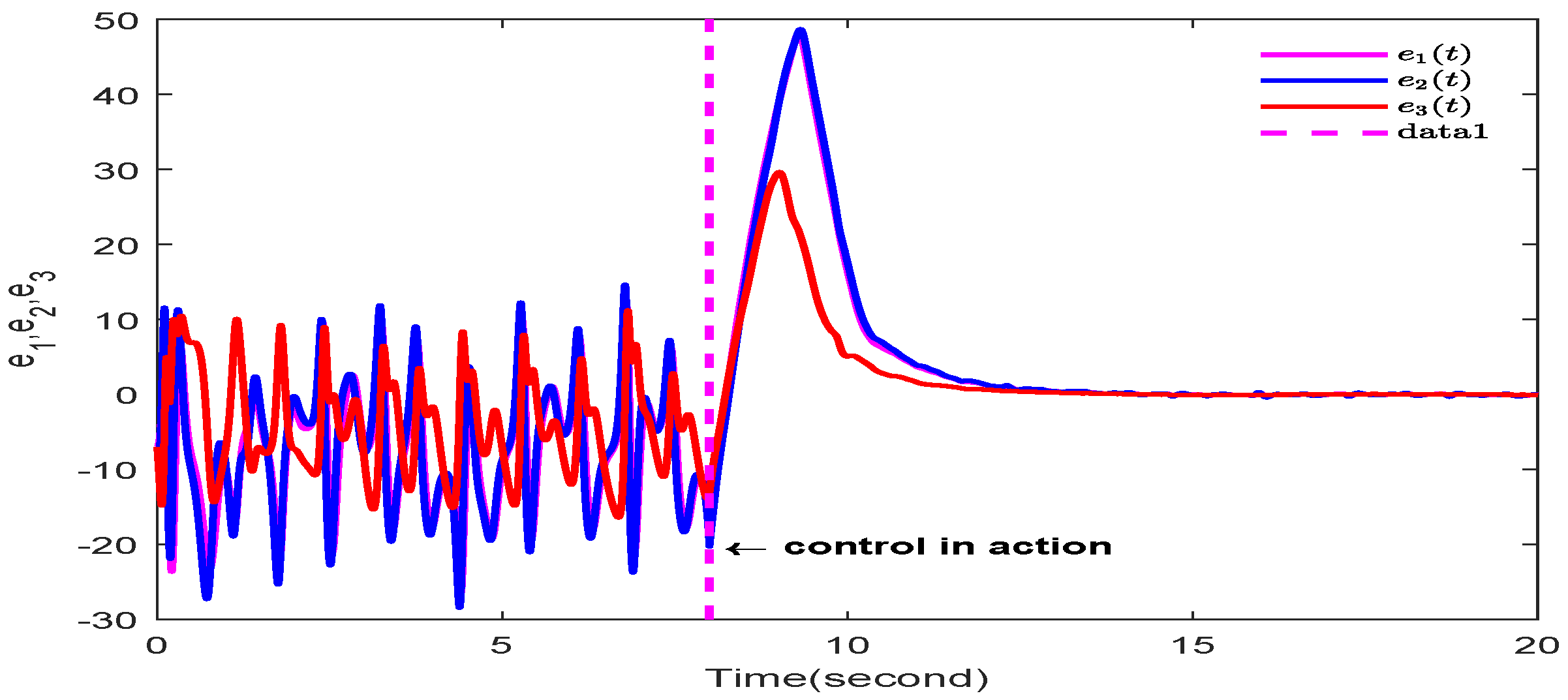
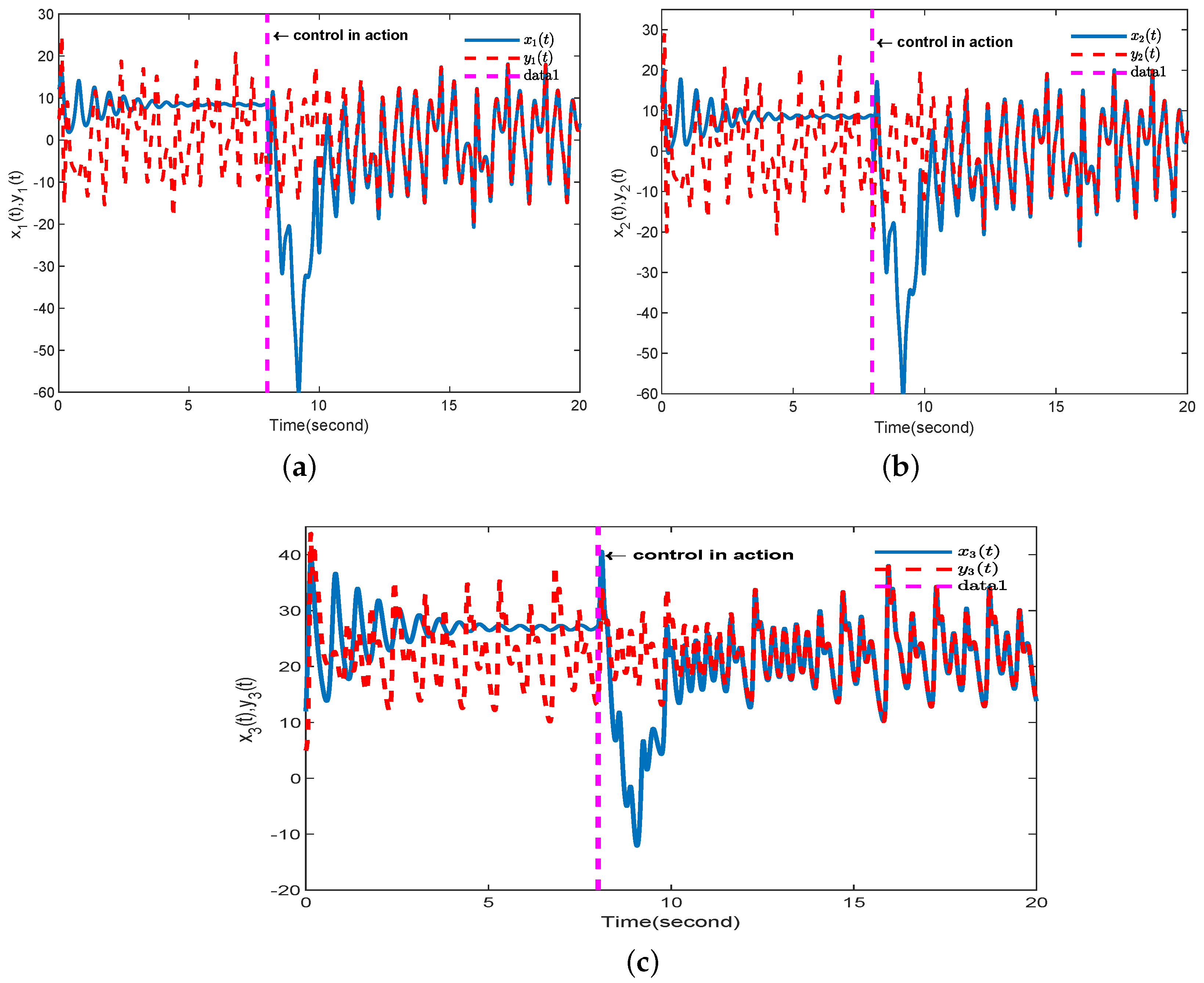
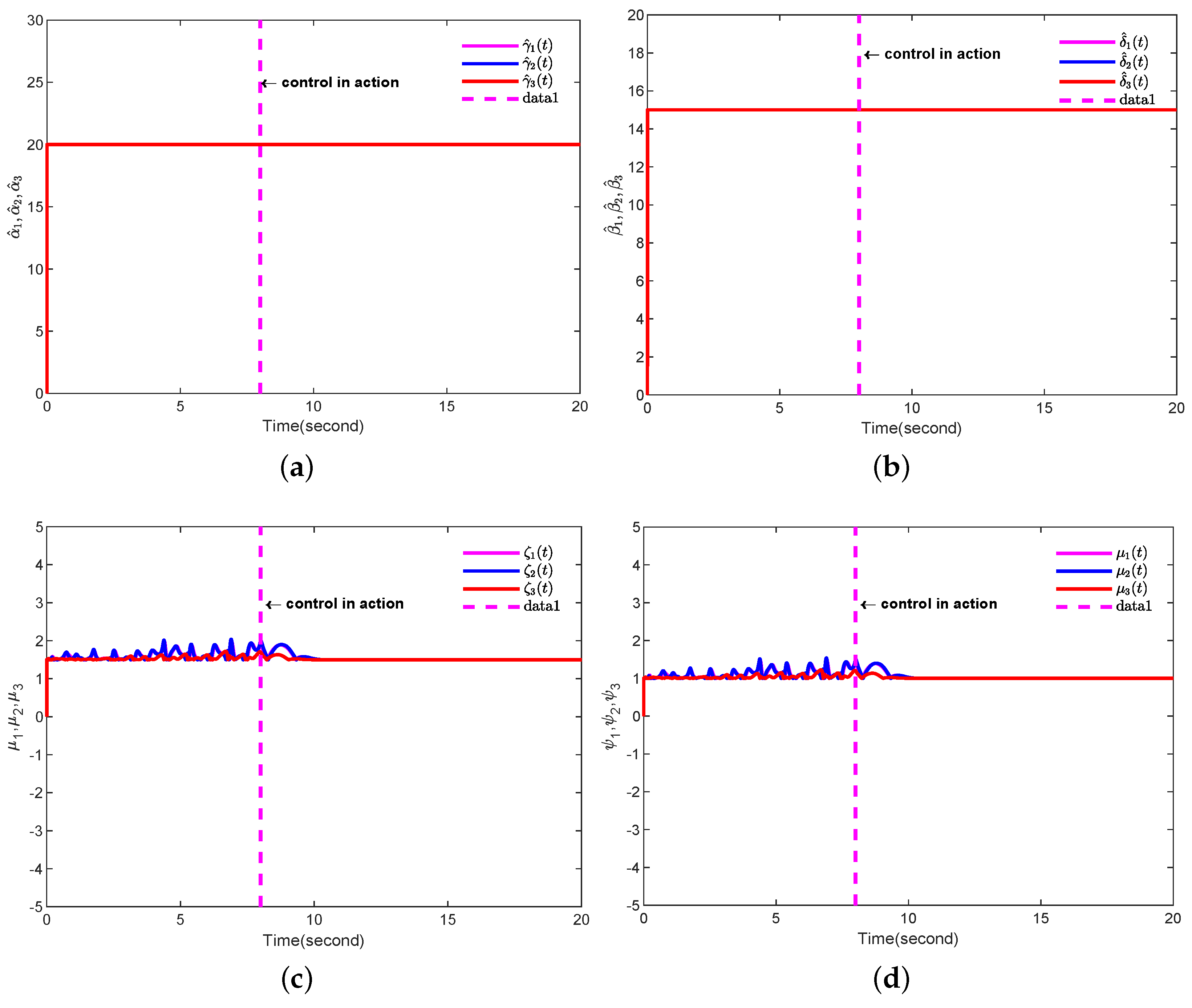
4. Simulation Results

In order to verify the validity of the proposed fractional-order ATSMC strategy, two simulation examples are given.
Example 1.
Using the proposed ATSMC method for the fractional-order Lorenz system and fractional-order Chen system: In order to facilitate the subsequent operations, uncertainties and disturbances are involved in the numerical simulation in the following forms, respectively.
f i ( y ) + d i f ( t ) = ψ i sin ( ρ i y i ) + θ i cos t , i = 1 , 2 , 3 ,
g i ( x ) + d i g ( t ) = ψ ^ i sin ( ρ i x i ) + θ ^ i cos t .
Suppose that the parameters are  ψ i = ψ ^ i = 0.5 ρ i = i π θ i = θ ^ i = 0.6 λ i = 0.3 ζ i = μ i p i = q i = 1 2 η = 1  and  M i = N i = 0.5 ; the initial values are  x i ( 0 ) = 10 y i ( 0 ) = 2 γ i ( 0 ) = 20 δ i ( 0 ) = 15 ζ i ( 0 ) = μ i ( 0 ) = 1  and  ν = κ = 0.95 ; and the fractional order is  α = 0.85 .
Phase diagrams of the fractional-order Lorenz system and fractional-order Chen system are shown in Figure 1, respectively. Therefore, let the primary system be
C h e n : D t α y 1 = 35 ( y 2 y 1 ) + f 1 ( y ) + d 1 f ( t ) , D t α y 2 = 28 y 2 7 y 1 y 1 y 3 + f 2 ( y ) + d 2 f ( t ) , D t α y 3 = y 1 y 2 3 y 3 + f 3 ( y ) + d 3 f ( t ) .
and the secondary system be
L o r e n z : D t α x 1 = 10 x 2 10 x 1 + g 1 ( x ) + d 1 g ( t ) + u 1 ( t ) , D t α x 2 = 28 x 1 x 2 x 1 x 3 + g 2 ( x ) + d 2 g ( t ) + u 2 ( t ) , D t α x 3 = x 1 x 2 8 3 x 3 + g 3 ( x ) + d 3 g ( t ) + u 3 ( t ) .
From (10) and (34)–(37), one obtains
D t α e 1 = 35 ( e 2 e 1 ) + 25 ( x 2 x 1 ) + 0.5 sin ( π y 1 ) + 0.5 s i n ( π x 1 ) + 1.2 cos t u 1 ( t ) , D t α e 2 = 7 y 1 28 x 1 + 28 y 2 + x 2 + x 1 x 3 y 1 y 3 + 0.5 sin ( 2 π y 2 ) + 0.5 sin ( 2 π x 2 ) + 1.2 cos t u 2 ( t ) , D t α e 3 = 3 y 3 + 8 3 x 3 x 1 x 2 + y 1 y 2 + 0.5 sin ( 3 π y 3 ) + 0.5 sin ( 3 π x 3 ) + 1.2 cos t u 3 ( t ) .
To emphasize the effect of the control action, this example applies the control input to the fifth second. The synchronization error of the FOCSs is shown in Figure 2. From the figure, it can be observed that the synchronization error converges to zero eventually, which indicates that the designed controller is effective. Figure 3 represents the chaos synchronization state trajectories between the Lorenz and Chen FOCSs. It can be seen that good tracking performance can be achieved, indicating that the designed control scheme is effective. Figure 4 shows the response of  γ ^ i δ ^ i ζ i  and  μ i  to time, which implies that the parameter change curve is bounded. Figure 5 depicts the time response of the controller  u i ( t ) . In Figure 5, as the sign function is replaced by tanh, the chattering phenomenon is significantly reduced, where  u ( t ) i l = ζ i tanh μ i s i . Additionally, the trajectory of  u i ( t )  tends to become smoother with increasing time t and almost no longer consumes energy, which implies the efficacy of our designed controller.
Example 2.
Considering fractional-order Rossler for the primary and secondary systems as follows.
P r i m a r y s y s t e m : D t α y 1 = y 2 + 5 y 1 + sin ( ρ 1 y 1 ) + cos t , D t α y 2 = y 3 y 1 + sin ( ρ 2 y 2 ) + cos t , D t α y 3 = y 3 ( y 2 10 ) + 1 + sin ( ρ 3 y 3 ) + cos t .
S e c o n d a r y s y s t e m : D t α x 1 = x 2 + 5 x 1 sin ( ρ 1 x 1 ) cos t + u 1 ( t ) , D t α x 2 = x 3 x 1 sin ( ρ 2 x 2 ) cos t + u 2 ( t ) , D t α x 3 = x 3 ( x 2 10 ) + 1 sin ( ρ 3 x 3 ) cos t + u 3 ( t ) .
The parameters are set as follows:  ρ i = i π λ i = 0.2 ζ i = μ i p i = q i = 1 2 η = 2 M i = N i = 0.65 x i ( 0 ) = 12 y i ( 0 ) = 5 γ i ( 0 ) = 25 δ i ( 0 ) = 20 ζ i ( 0 ) = μ i ( 0 ) = 1.5 ν = κ = 0.85  and  α = 0.95 .
Furthermore, the error dynamics are obtained as follows:
D t α e 1 = e 2 + 5 e 1 + sin ( π y 1 ) + s i n ( π x 1 ) + 2 cos t u 1 ( t ) , D t α e 2 = e 3 e 1 + sin ( 2 π y 2 ) + sin ( 2 π x 2 ) + 2 cos t u 2 ( t ) , D t α e 3 = y 3 y 2 x 3 x 2 10 e 3 + sin ( 3 π y 3 ) + sin ( 3 π x 3 ) + 2 cos t u 3 ( t ) .
The simulation results are shown in Figure 6, Figure 7 and Figure 8. The dynamic trajectory of synchronization error for FOCSs is shown in Figure 6. As shown in the figure, as time t approaches infinity, the error tends toward zero. Figure 7 depicts the state synchronization between the primary system and the secondary system, which indicates that the controller can work well. The time response of the adaptive parameters is shown in Figure 8, and they are bounded.

5. Conclusions

In this paper, an ATSMC scheme is used to solve the synchronization control of a class of uncertain FOCSs with disturbances. First of all, a smooth fractional-order non-singular sliding surface is designed to effectively reduce the chattering phenomenon. Then, a terminal sliding-mode synchronization controller is proposed to improve the convergence rate of the tracking error and ensure that the tracking error can converge to the origin in a finite time. Finally, the effectiveness and applicability of the proposed fractional-order finite-time ATSMC method can be verified by the Lyapunov stability analysis and simulation results. However, the upper bounds of uncertainties and disturbances for uncertain FOCSs considered in this paper are known. Therefore, further research will be aimed at determining how to use the fractional-order ATSMC method to solve uncertain FOCSs with unknown upper bounds and further reduce the chattering phenomenon and improve convergence speed through this technology.

Funding

This work was supported by the National Natural Science Foundation of China (Grant No. 11302184), the Xiamen Industry University Research Project (Grant No. 2023CXY0426), and the Fujian Provincial Natural Science Foundation (Grant No. 2021J011194).

Data Availability Statement

All data used are included in the article.

Conflicts of Interest

The authors declare that they have no competing financial interests or personal relationships that could have appeared to influence the work reported in this article.

References

  1. Liu, T.; Yan, H.; Banerjee, S.; Mou, J. A fractional-order chaotic system with hidden attractor and self-excited attractor and its DSP implementation. Chaos Solitons Fractals 2021, 145, 110791. [Google Scholar] [CrossRef]
  2. Wang, H.; Weng, C.; Song, Z.; Cai, J. Research on the law of spatial fractional calculus diffusion equation in the evolution of chaotic economic system. Chaos Solitons Fractals 2020, 131, 109462. [Google Scholar] [CrossRef]
  3. Sene, N. Introduction to the fractional-order chaotic system under fractional operator in Caputo sense. Alex. Eng. J. 2021, 60, 3997–4014. [Google Scholar] [CrossRef]
  4. Baleanu, D.; Zibaei, S.; Namjoo, M.; Jajarmi, A. A nonstandard finite difference scheme for the modeling and nonidentical synchronization of a novel fractional chaotic system. Adv. Differ. Equ. 2021, 2021, 308. [Google Scholar] [CrossRef]
  5. Balootaki, M.A.; Rahmani, H.; Moeinkhah, H.; Mohammadzadeh, A. On the synchronization and stabilization of fractional-order chaotic systems: Recent advances and future perspectives. Phys. A Stat. Mech. Its Appl. 2020, 551, 124203. [Google Scholar] [CrossRef]
  6. Qi, F.; Qu, J.; Chai, Y.; Chen, L.; Lopes, A.M. Synchronization of incommensurate fractional-order chaotic systems based on linear feedback control. Fractal Fract. 2022, 6, 221. [Google Scholar] [CrossRef]
  7. Mobayen, S.; Pujol-Vázquez, G. A robust LMI approach on nonlinear feedback stabilization of continuous state-delay systems with Lipschitzian nonlinearities: Experimental validation. Iran. J. Sci. Technol. Trans. Mech. Eng. 2019, 43, 549–558. [Google Scholar] [CrossRef]
  8. Luo, S.; Lewis, F.L.; Song, Y.; Vamvoudakis, K.G. Adaptive backstepping optimal control of a fractional-order chaotic magnetic-field electromechanical transducer. Nonlinear Dyn. 2020, 100, 523–540. [Google Scholar] [CrossRef]
  9. Dalir, M.; Bigdeli, N. An adaptive neuro-fuzzy backstepping sliding mode controller for finite time stabilization of fractional-order uncertain chaotic systems with time-varying delays. Int. J. Mach. Learn. Cybern. 2021, 12, 1949–1971. [Google Scholar] [CrossRef]
  10. Qiu, H.; Liu, H.; Zhang, X. Composite adaptive fuzzy backstepping control of uncertain fractional-order nonlinear systems with quantized input. Int. J. Mach. Learn. Cybern. 2023, 14, 833–847. [Google Scholar] [CrossRef]
  11. Li, Y.; Yang, T.; Tong, S. Adaptive neural networks finite-time optimal control for a class of nonlinear systems. IEEE Trans. Neural Netw. Learn. Syst. 2019, 31, 4451–4460. [Google Scholar] [CrossRef] [PubMed]
  12. Luo, R.; Huang, M.; Su, H. Robust control and synchronization of 3-D uncertain fractional-order chaotic systems with external disturbances via adding one power integrator control. Complexity 2019, 2019, 8417536. [Google Scholar] [CrossRef]
  13. Kiruthika, R.; Krishnasamy, R.; Lakshmanan, S.; Prakash, M.; Manivannan, A. Non-fragile sampled-data control for synchronization of chaotic fractional-order delayed neural networks via LMI approach. Chaos Solitons Fractals 2023, 169, 113252. [Google Scholar] [CrossRef]
  14. Al-Raeei, M. Applying fractional quantum mechanics to systems with electrical screening effects. Chaos Solitons Fractals 2021, 150, 111209. [Google Scholar] [CrossRef]
  15. Stankevich, N.; Volkov, E. Chaos–hyperchaos transition in three identical quorum-sensing mean-field coupled ring oscillators. Chaos Interdiscip. J. Nonlinear Sci. 2021, 31. [Google Scholar] [CrossRef] [PubMed]
  16. Rong, C.; Zhang, B. Fractional electromagnetic waves in circular waveguides with fractional-order inductance characteristics. J. Electromagn. Waves Appl. 2019, 33, 2142–2154. [Google Scholar] [CrossRef]
  17. Hao, Y.; Huang, C.; Cao, J.; Liu, H. Positivity and Stability of Fractional-Order Linear Time-Delay Systems. J. Syst. Sci. Complex. 2022, 35, 2181–2207. [Google Scholar] [CrossRef]
  18. Ghanbari, B. On the modeling of the interaction between tumor growth and the immune system using some new fractional and fractional-fractal operators. Adv. Differ. Equ. 2020, 2020, 1–32. [Google Scholar] [CrossRef]
  19. Qiu, H.; Wang, H.; Pan, Y.; Cao, J.; Liu, H. Stability and Lgain of Positive Fractional-Order Singular Systems With Time-Varying Delays. IEEE Trans. Circuits Syst. II Express Briefs 2023, 70, 3534–3538. [Google Scholar] [CrossRef]
  20. Norouzi, B.; Mirzakuchaki, S. Breaking a novel image encryption scheme based on an improper fractional order chaotic system. Multimed. Tools Appl. 2017, 76, 1817–1826. [Google Scholar] [CrossRef]
  21. Ma, Z.; Ma, H. Reduced-order observer-based adaptive backstepping control for fractional-order uncertain nonlinear systems. IEEE Trans. Fuzzy Syst. 2019, 28, 3287–3301. [Google Scholar] [CrossRef]
  22. Feng, T.; Wang, Y.E.; Liu, L.; Wu, B. Observer-based event-triggered control for uncertain fractional-order systems. J. Frankl. Inst. 2020, 357, 9423–9441. [Google Scholar] [CrossRef]
  23. Naik, P.A.; Zu, J.; Owolabi, K.M. Global dynamics of a fractional order model for the transmission of HIV epidemic with optimal control. Chaos Solitons Fractals 2020, 138, 109826. [Google Scholar] [CrossRef] [PubMed]
  24. Zhang, L.; Yang, Y. Impulsive effects on bipartite quasi synchronization of extended Caputo fractional order coupled networks. J. Frankl. Inst. 2020, 357, 4328–4348. [Google Scholar] [CrossRef]
  25. Rajagopal, K.; Panahi, S.; Chen, M.; Jafari, S.; Bao, B. Suppressing spiral wave turbulence in a simple fractional-order discrete neuron map using impulse triggering. Fractals 2021, 29, 2140030. [Google Scholar] [CrossRef]
  26. You, X.; Shi, M.; Guo, B.; Zhu, Y.; Lai, W.; Dian, S.; Liu, K. Event-triggered adaptive fuzzy tracking control for a class of fractional-order uncertain nonlinear systems with external disturbance. Chaos Solitons Fractals 2022, 161, 112393. [Google Scholar] [CrossRef]
  27. Hao, Y.; Fang, Z.; Liu, H. Stabilization of delayed fractional-order T-S fuzzy systems with input saturations and system uncertainties. Asian J. Control 2023, 26, 246–264. [Google Scholar] [CrossRef]
  28. Jiang, J.; Cao, D.; Chen, H. Sliding mode control for a class of variable-order fractional chaotic systems. J. Frankl. Inst. 2020, 357, 10127–10158. [Google Scholar] [CrossRef]
  29. Modiri, A.; Mobayen, S. Adaptive terminal sliding mode control scheme for synchronization of fractional-order uncertain chaotic systems. ISA Trans. 2020, 105, 33–50. [Google Scholar] [CrossRef]
  30. Rabah, K.; Ladaci, S. A fractional adaptive sliding mode control configuration for synchronizing disturbed fractional-order chaotic systems. Circuits Syst. Signal Process. 2020, 39, 1244–1264. [Google Scholar] [CrossRef]
  31. Song, C.; Fei, S.; Cao, J.; Huang, C. Robust synchronization of fractional-order uncertain chaotic systems based on output feedback sliding mode control. Mathematics 2019, 7, 599. [Google Scholar] [CrossRef]
  32. Wang, R.; Zhang, Y.; Chen, Y.; Chen, X.; Xi, L. Fuzzy neural network-based chaos synchronization for a class of fractional-order chaotic systems: An adaptive sliding mode control approach. Nonlinear Dyn. 2020, 100, 1275–1287. [Google Scholar] [CrossRef]
  33. Khan, A.; Nasreen; Jahanzaib, L.S. Synchronization on the adaptive sliding mode controller for fractional order complex chaotic systems with uncertainty and disturbances. Int. J. Dyn. Control 2019, 7, 1419–1433. [Google Scholar] [CrossRef]
  34. Labbaf Khaniki, M.A.; Salehi Kho, M.; Aliyari Shoorehdeli, M. Control and synchronization of chaotic spur gear system using adaptive non-singular fast terminal sliding mode controller. Trans. Inst. Meas. Control 2022, 44, 2795–2808. [Google Scholar] [CrossRef]
  35. Shao, S.; Chen, M.; Yan, X. Adaptive sliding mode synchronization for a class of fractional-order chaotic systems with disturbance. Nonlinear Dyn. 2016, 83, 1855–1866. [Google Scholar] [CrossRef]
  36. Almatroud, A.O. Synchronisation of two different uncertain fractional-order chaotic systems with unknown parameters using a modified adaptive sliding-mode controller. Adv. Differ. Equ. 2020, 2020, 1–14. [Google Scholar] [CrossRef]
  37. Mirrezapour, S.Z.; Zare, A.; Hallaji, M. A new fractional sliding mode controller based on nonlinear fractional-order proportional integral derivative controller structure to synchronize fractional-order chaotic systems with uncertainty and disturbances. J. Vib. Control 2022, 28, 773–785. [Google Scholar] [CrossRef]
  38. Giap, V.N.; Nguyen, Q.D.; Trung, N.K.; Huang, S.C.; Trinh, X.T. Disturbance observer based on terminal sliding-mode control for a secure communication of fractional-order takagi-sugeno fuzzy chaotic systems. In Proceedings of the International Conference on Advanced Mechanical Engineering, Automation and Sustainable Development, Ha Long, Vietnam, 4–7 November 2021; Springer: Cham, Switzerland, 2021; pp. 936–941. [Google Scholar]
  39. Sweilam, N.; Khader, M.; Al-Bar, R. Numerical studies for a multi-order fractional differential equation. Phys. Lett. A 2007, 371, 26–33. [Google Scholar] [CrossRef]
  40. Dai, H.; Chen, W. New power law inequalities for fractional derivative and stability analysis of fractional order systems. Nonlinear Dyn. 2017, 87, 1531–1542. [Google Scholar] [CrossRef]
  41. Aghababa, M.P.; Akbari, M.E. A chattering-free robust adaptive sliding mode controller for synchronization of two different chaotic systems with unknown uncertainties and external disturbances. Appl. Math. Comput. 2012, 218, 5757–5768. [Google Scholar] [CrossRef]
  42. Wei, X.; Liu, D.Y.; Boutat, D. Nonasymptotic pseudo-state estimation for a class of fractional order linear systems. IEEE Trans. Autom. Control 2017, 62, 1150–1164. [Google Scholar] [CrossRef]
  43. Lee, H.; Utkin, V.I. Chattering suppression methods in sliding mode control systems. Annu. Rev. Control 2007, 31, 179–188. [Google Scholar] [CrossRef]
Figure 1. The state and motion trajectory of Lorenz and Chen FOCSs. (a) Phase diagram of the Lorenz FOCS and state (37); (b) phase diagram of the Chen FOCS and state (36).
Fractalfract 08 00188 g001
Figure 2. Trajectory of synchronization error of Lorenz and Chen FOCSs.
Fractalfract 08 00188 g002
Figure 3. Synchronization trajectory of the states of Lorenz and Chen FOCSs. (a x 1 y 1 ; (b x 2 y 2 ; (c x 3 y 3 .
Fractalfract 08 00188 g003
Figure 4. Trajectory of adaptive parameters. (a γ ^ i ; (b δ ^ i ; (c ζ i ; (d μ i .
Fractalfract 08 00188 g004
Figure 5. Trajectory of  u l ( t ) .
Fractalfract 08 00188 g005
Figure 6. Trajectory of synchronization error of FOCSs.
Fractalfract 08 00188 g006
Figure 7. Synchronization trajectory of states of FOCSs. (a x 1 y 1 ; (b x 2 y 2 ; (c x 3 y 3 .
Fractalfract 08 00188 g007
Figure 8. Adaptive parameters. (a γ ^ i ; (b δ ^ i ; (c ζ i ; (d μ i .
Fractalfract 08 00188 g008
Table 1. Symbol descriptions.
SymbolDescription
ATSMCAdaptive terminal sliding-mode control
FOCSFractional-order chaotic system
SMCSliding-mode control
  R Real number space
  Γ ( · ) Gamma function
  R n n-dimensional vectors space
  | | · | | 1 First norm
Disclaimer/Publisher’s Note: The statements, opinions and data contained in all publications are solely those of the individual author(s) and contributor(s) and not of MDPI and/or the editor(s). MDPI and/or the editor(s) disclaim responsibility for any injury to people or property resulting from any ideas, methods, instructions or products referred to in the content.

