Error-Based Switched Fractional Order Model Reference Adaptive Control for MIMO Linear Time Invariant Systems

Abstract

This paper presents the design and analysis of Switched Fractional Order Model Reference Adaptive Controllers (SFOMRAC) for Multiple Input Multiple Output (MIMO) linear systems with unknown parameters. The proposed controller uses adaptive laws whose derivation order switches between a fractional order and the integer order, according to a certain level of control error. The switching aims to use fractional orders when the control error is larger to improve transient response and system performance during large disturbed states, and to obtain smoother control signals, leading to a better control energy usage. Then, it switches to the integer order when the control error is smaller to improve steady state. Boundedness of all the signals in the scheme is analytically proved, as well as convergence of the control error to zero. Moreover, these properties are extended to the case when system states are affected by a bounded non-parametric disturbance. Simulation studies are carried out using different representative plants to be controlled, showing that fractional orders and switching error levels can be found in most of the cases, such as when SFOMRAC achieves a better balance among control energy and system performance than the non-switched equivalent strategies.

1. Introduction

In the context of energy efficiency of today’s world, one of the challenges that industry needs to address is related to the use of automatic control strategies that not only prioritizes improvements in the process behavior, but also takes into account the energy used to make it controlled. In this searching for improvements in controlled systems, fractional operators (e.g., integrals and derivatives of real orders [1]) have started being used in the design and implementation of control strategies, resulting in generalized controllers with reported advantages such as better management of noise [2], better behavior under disturbances and improvements in transient responses [3,4], among others, as compared to the non-fractional equivalent strategies. Smoother control signals have been also reported as an advantage of using fractional operators inside controllers, which is often related to a lower control energy. We can cite, for instance, the work [5], where authors reported that the use of a Fractional Order Proportional Integral Derivative (FOPID) controller produced a significantly smaller control signal than the classic Proportional Integral Derivative (PID) controller, which would save energy for the actuator. Also, in [6], authors reported a lower control energy used when a Fractional Order Sliding Model Control (FOSMC) was applied to an energy harvesting system, compared to the classic non-integer case. In [7], on the other hand, Model Reference Adaptive Control (MRAC) schemes were presented, using orders for the adaptive laws in the interval $(0,1]$, which were obtained through Particle Swarm Optimization. Results showed that when the control energy was included in the objective function, the resulting orders were fractional or combinations of fractional and integer orders, suggesting that the use of fractional adaptive laws could play an important role in the control energy management.

However, when comparing fractional order controllers to their equivalent integer order controllers, trade-offs usually arise among some system performance metrics. For instance, when FOPID are used, a faster response in the transient state with lower overshoots and higher flexibility to parameter variations has been reported, compared to those obtained with the classic PID controller. However, the steady state can be deteriorated with the FOPID, while the PID usually gives good steady state performance (see [8,9,10] and the references therein). To deal with these trade-offs, switched controllers have been proposed, where the PID (or PI) controller is used in steady state and the FOPID (or FOPI) controller is used during the transient stage, aiming to take advantage of each controller’s strengths. The design, tuning and application of these switched controllers have been reported in [8] to regulate the DC-link voltage of a single phase active power filter and in [9,10] to extract maximum power under fluctuating wind speed for grid connected wind energy conversion system. In all cases, the switching mechanism is based on the current value of the control error. Boundedness of the signals and convergence of the control error to zero are not analytically proved in any case.

When dealing with Fractional Order Model Reference Adaptive Controllers (FOMRAC), it has been observed that the use of fractional order adaptive laws can lead to lower control energy, compared to the classic Model Reference Adaptive Control (MRAC), but the convergence speed of the control error tends to decrease, deteriorating the steady state (see [7,11] and the discussion and references therein). In an attempt to overcome this trade-off, a Switched Fractional Order Model Reference Adaptive Control (SFOMRAC) scheme was proposed (see, for instance, [11]) to control linear time invariant systems. The adaptive laws to estimate controller parameters were fractional order differential equations whose derivation order switched between a real number in the interval $\left(0,1\right)$ and 1, at some time instant of the transient response (time-based switching), which can be seen as switching between a SFOMRAC scheme and an MRAC scheme. The work in [11] presented exhaustive simulation studies, using time-based SFOMRAC schemes to control first order plants (stable and unstable). The controller parameters were tested in wide ranges: fractional orders in the whole interval $\left(0,2\right)$, switching times selected across the entire transient, different values of adaptive gains $\gamma$ and fast and slow reference models. The analysis of the results showed that for every plant and reference model tested, SFOMRAC controlled systems have better performance with respect to indices that emphasize and penalize longer-lasting and larger errors than the non-switched cases, and many times, they also demonstrated lower control energy consumption. As far as the authors know, no other works have been published dealing with SFOMRAC schemes, apart from those published by the authors of this paper.

As promising as these results may seem, still, there are two main drawbacks of the schemes proposed in [11]. First, a time-based switching is difficult to design in practice because the system is unknown in advance, and thus, the choice of the switching time becomes arbitrary. The condition for switching should depend on system variables that can be measured and represent how well the control is doing. Second but not least, analytical proof of stability and convergence in [11] relies on the fact that only one switch is allowed, imposing conditions in advance on an unknown system. These drawbacks are addressed in this paper, leading to its main contributions as stated in the following.

• This paper proposes an error-based switching mechanism in the design of SFOMRAC schemes for LTI systems. The switching uses the value of the control error to decide whether to use the fractional order or the integer order in the controller parameters adaptive laws. Compared to the previous work [11], the error-based switching is more appealing in practice because it allows for making decisions based on a system signal that can be measured and used as a metric of system performance and stability.
• The SFOMRAC is proposed in this paper for multivariable systems. This is an improvement regarding previous works ([11] and references therein), where only single input, single output systems were considered.
• A complete and thorough analytical proof of stability and convergence of the resulting design is provided in this paper, where the controller will not be limited in advance to switching by a finite amount, as it was in previous works ([11] and some references therein).
• The design and analysis is also carried out for cases when system states are affected by a bounded non-parametric disturbance. This non-ideal case was not addressed in any of the previous works.
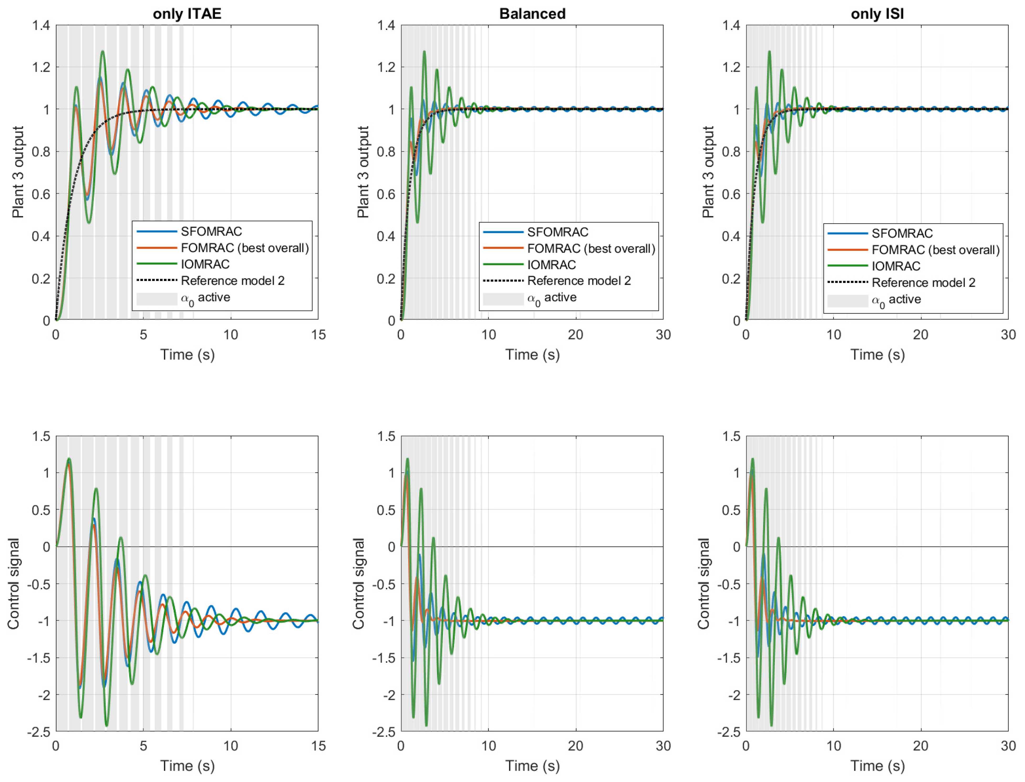
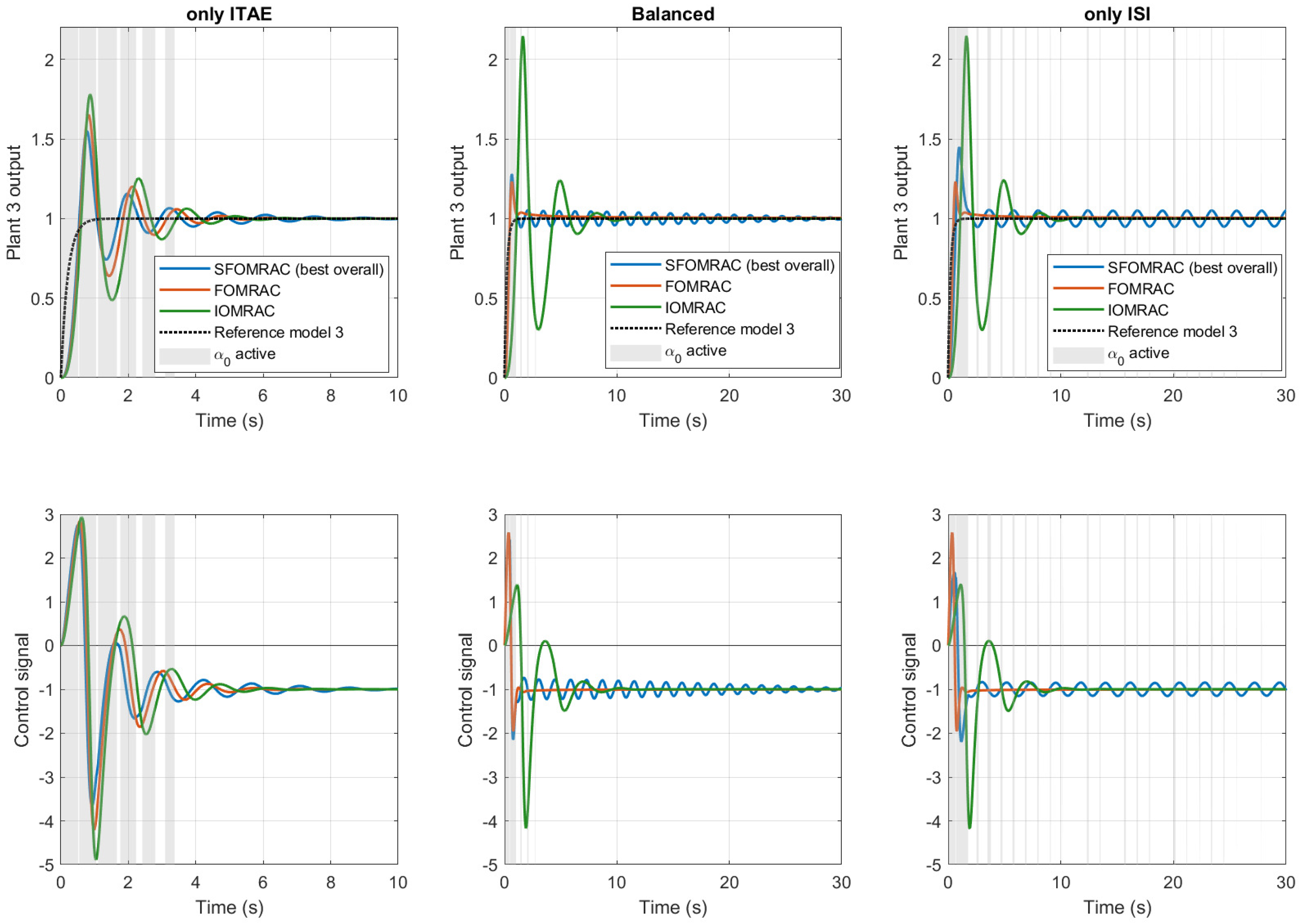
• Exhaustive simulation studies are conducted, and numerical results show that the SFOMRAC allows for obtaining a better balance among performance indicator ITAE (Integral of the Time weighted Absolute value of the Error) and control energy ISI (Integral of the Squared Control Signal) for some switching error levels, leading to an improved control strategy compared to the classical non-switched integer-order (MRAC) and fractional-order (FOMRAC) schemes.

The paper is organized as follows. Section 2 introduces some basic definitions, lemmas and theorems used within the paper. Section 3 presents the control problem, the proposed SFOMRAC scheme and the analytical proof of stability and convergence of the signals in the controlled scheme. Section 4 presents the results of exhaustive simulation studies, using the proposed SFOMRAC scheme for different first order LTI systems, and varying several design parameters in a wide range, leading to discussion and conclusions about their influence in the control energy and the system behavior.

2. Basic Concepts

This section presents definitions, lemmas and theorems that are used within the paper.

2.1. Notation and Basic Definitions

In this note, ${\mathbb{R}}_{>(\ge )0}$ is the set of positive (non-negative) real numbers, and ${\mathbb{R}}^n$ is the Euclidean space of dimension n. For $x\in {\mathbb{R}}^n$ and $A\in {\mathbb{R}}^{n\times n}$, a positive definite matrix, ${\left|x\right|}_A:=x^{\top }Ax$ defines a norm. We extend this definition to matrices, i.e., ${\left|B\right|}_A:=B^{\top }AB$ for $B\in {\mathbb{R}}^{n\times n}$.

2.2. Elements of Fractional Calculus

Fractional calculus is a generalization of traditional calculus by considering integrals and derivatives of orders that can be any real or complex numbers [1]. The Riemann-Liouville fractional integral of a function $f:\mathbb{R}\to \mathbb{R}$ is one of the main concepts of fractional calculus, defined as follows.

Definition 1 

(Riemann–Liouville fractional integral [12]).

$$I_a^{\alpha }f\left(t\right):=\frac{1}{\Gamma \left(\alpha \right)}\underset{a}{\overset{t}{\int }}{\left(t-\tau \right)}^{\alpha -1}f\left(\tau \right)d\tau ,$$

(1)

where $\alpha >0$ and $\Gamma \left(\alpha \right)=\underset{0}{\overset{\infty }{\int }}{t}^{\alpha -1}{e}^{-t}dt$ is the Gamma function [1].

Referring to definitions of fractional derivatives, different alternatives can be found in technical literature. This paper uses the Caputo definition for the fractional derivative, which corresponds to

Definition 2 

(Caputo fractional derivative [12]).

$$D_a^{\alpha }f\left(t\right):=I_a^{m-\alpha }{D}^{m}f\left(t\right),$$

(2)

where $\alpha >0$ and $m=⌈\alpha ⌉$.

2.3. Analytical Tools

Property 1. 

For any continuous function $f:[0,\infty )\to \mathbb{R}$, any real numbers $a,\alpha ,\beta >0$, and for any real number $t>0$, the following holds [12]:

$$\begin{array}{c}\hfill I_a^{\alpha }{I}_a^{\beta }f\left(t\right)=I_a^{\alpha +\beta }f\left(t\right),\end{array}$$

(3)

and

$$\begin{array}{c}\hfill I_a^{\alpha }{D}_a^{\alpha }f\left(t\right)=f\left(t\right)-f\left(a\right).\end{array}$$

(4)

The following result establishes existence and uniqueness in the set of continuous functions for the solutions of a kind of fractional equation.

Theorem 1 

([13]). Consider the system of fractional order integral equations

$$y\left(t\right)=p\left(t\right)+I^{\alpha }\left[f(.,y(.))\right]\left(t\right),$$

(5)

where α is to be seen as a vector with components ${\alpha }_i$, and y, f, p are vectors of components $y_i$, $f_i$, $p_i$, respectively, for $i=1,\dots ,n$. If $p:[0,T]\to {\mathbb{R}}^n$ is a continuous function and $f_i(.,.)$ are continuous functions in their first variable and Lipschitz continuous functions in their second variables for $i=1,\dots ,n$, then

i.

There exists a unique continuous solution $y\in \mathcal{C}[0,T]$ for system (5).

ii.

$y\in \mathcal{C}[0,T]$ is a solution for system (5) for

$$p_i\left(t\right):=\sum _{k=0}^{⌈\alpha ⌉-1}\frac{t_k}{k!}{y}_{i_0}^{\left(k\right)}$$

(6)

if and only if each of its components $y_i$ is a solution to $D^{{\alpha }_i}{y}_i=f_i(t,y)$ with initial condition $y_i^{\left(k\right)}\left(0\right)=y_{i_0}^{\left(k\right)}$ for $k=1,\dots ,⌈\alpha ⌉-1$ and $i=1,\dots ,n$.

Finally, a useful property for the derivative of composite functions is presented.

Theorem 2 

([14]). For a given $x\in {\mathbb{R}}^d$, let $u\in \left\{x\right\}+I_{0+}^{\alpha }\mathcal{C}\left([0,T]\right),{\mathbb{R}}^d$ and $V:{\mathbb{R}}^d\to \mathbb{R}$ satisfies the following conditions

• The function V is convex on ${\mathbb{R}}^d$ and $V\left(0\right)=0$.
• The function V is differentiable on ${\mathbb{R}}^d$.

Then, the following inequality holds for all $t\in [0,T]$:

$$D_{0+}^{\alpha }V\left(u\left(t\right)\right)\le \langle \nabla V\left(u\left(t\right)\right),D_{0+}^{\alpha }u\left(t\right)\rangle .$$

(7)

3. Problem Statement and Proposed Control Scheme

Although most of the real processes that need to be controlled are nonlinear and time varying, linearization around operating points is still widely used to deal with the design of control strategies [15,16]. This is because it is very common for industrial processes to operate in certain regions where their behavior can be approximated as linear and time invariant. For this reason, the development of control strategies for LTI systems is still widely addressed. In what follows, the problem of controlling an LTI system with unknown parameters is presented, together with the proposed switched fractional order controller structure.

3.1. Control Problem

Let us consider a multi-input, multi-output linear time invariant plant described by

$${\dot{x}}_p\left(t\right)=A_p{x}_p\left(t\right)+B_{p}u\left(t\right),x_p\left(0\right)=x_{p_0}\in {\mathbb{R}}^n,$$

(8)

where $A_p\in {\mathbb{R}}^{n\times n}$ and $B_p\in {\mathbb{R}}^{n\times q}$ are unknown constant matrices, $u\in {\mathbb{R}}^q$ is the input of the system and $x_p\in {\mathbb{R}}^n$ is the state, which is assumed to be accessible.

An asymptotically stable reference model is specified by the linear time-invariant system described by

$${\dot{x}}_m\left(t\right)=A_m{x}_m\left(t\right)+B_{m}r\left(t\right),x_m\left(0\right)=x_{m_0}\in {\mathbb{R}}^n,$$

(9)

where $r\in {\mathbb{R}}^q$ is a bounded ${\mathcal{C}}^1$ reference input, $A_m\in {\mathbb{R}}^{n\times n},B_m\in {\mathbb{R}}^{n\times q}$ are known matrices and $A_m$ is a Hurwitz matrix, e.g., a square matrix whose eigenvalues have negative real parts.

The control problem corresponds to defining a control signal u such that $x_p$ asymptotically follows $x_m$ and all the closed-loop signals remain bounded. The reference model of course is a designer choice and will be selected such as its state $x_m\left(t\right)$ will represent the desired trajectory for the plant state $x_p\left(t\right)$.

To ensure the solvability of this problem, we make the following assumptions dealing with the controllability of the system (8). The first one is known as the matching condition [15].

Assumption 1. 

There exist constant matrices $L^{*}\in {\mathbb{R}}^{q\times q}$ and $K^{*}\in {\mathbb{R}}^{q\times n}$ such that

$$B_m=B_p{L}^{*},A_p+B_p{K}^{*}=A_m.$$

(10)

The second one is the generalization of requesting the control direction constant and known.

Assumption 2. 

$L^{*}$ is either positive or negative definite, the sign of which is assumed known and, without loss of generality, taken positive.

Both Assumptions 1 and 2 are standard in the literature [15]. Though our contribution is not to relax them, we indicate that the second can be weakened using Nussbaum gains.

This control problem has been solved in the past using several control strategies, such as direct MRAC, indirect algebraic MRAC, indirect dynamic MRAC, combined MRAC [16], among others. In these cases, the control signal usually uses parameters that are estimated using adaptive laws in the form of integer order differential equations. Fractional order generalizations of some of these control strategies have been proposed as well (see for instance [3]), where the main difference is that adaptive laws are in the form of fractional order differential equations and the tracking error has not been proved to converge to zero without an additional hypothesis on r. More recently, switched fractional order adaptive laws have been proposed as well [11] in an attempt to achieve a better balance among system behavior and control energy, while the error is shown to converge to zero. However, the proposed switching strategy is not practical because it does not depend on a measurable system variable. Also, it imposes some restrictive conditions on the number of switching without deeper analysis. In what follows, an alternative switching strategy is proposed, which aims to overcome those drawbacks.

3.2. Proposed Control Strategy

Let us choose the certainty equivalent control structure defined as

$$u\left(t\right)=K\left(t\right)x_p\left(t\right)+L\left(t\right)r\left(t\right),t\ge 0$$

(11)

with $K,L$ estimations of $K^{*},L^{*}$ adjusted by using the following switched fractional order adaptive law.

$$\begin{array}{ccc}\hfill D_{a\left(t\right)}^{\alpha \left(t\right)}K\left(t\right)& =& -{\gamma }_1{B}_{m}Pe\left(t\right)x_p{\left(t\right)}^{\top },K\left(0\right)=K_0\hfill \\ \hfill D_{a\left(t\right)}^{\alpha \left(t\right)}L\left(t\right)& =& -{\gamma }_2{B}_{m}Pe\left(t\right)r{\left(t\right)}^{\top },L\left(0\right)=L_0\hfill \end{array}$$

(12)

where $e\left(t\right)=x_p\left(t\right)-x_m\left(t\right)$ is the control error, $P\in {\mathbb{R}}^{n\times n}$ is a symmetric positive definite matrix such that $A_m^{T}P+P{A}_m=-Q$, with $Q\in {\mathbb{R}}^{n\times n}$ being an arbitrary positive definite matrix. The existence of such P is ensured by the Hurwitz property of $A_m$. The fractional order $\alpha \left(t\right)$ is varied using the following switched strategy for any $t>0$ with

$$\alpha \left(t\right)=\left\{\begin{array}{ccc}{\alpha }_0\hfill & if& ||e\left(t\right)||>ϵ\mathrm{and}h\left(t\right)\\ \\ 1\hfill & if& \mathrm{otherwise}\end{array}\right.,$$

(13)

where $ϵ>0$ and ${\alpha }_0\in (0,1)$ are designer choices, and it is implicit that the switch occurs whenever $L\in {\mathbb{R}}^{q\times q}$ and $K\in {\mathbb{R}}^{q\times n}$, as, otherwise, the solution is not defined. The function $h(·)$ is a logic function (i.e., taking true/false values) encoding, on the one hand, a hysteresis mechanism to avoid Zeno solutions, and on the other, a mechanism stressing the spirit behind (13), namely, that in disturbed or transient stages ($||e||>ϵ$), the adaptation with ${\alpha }_0$ is needed, and conversely, that when staying close to the aim ($||e||<ϵ$), the lesser should be the need of switching to ${\alpha }_0$.

In detail, by fixing a small enough $\delta >0$, the hysteresis will be implemented by switching from the integer mode to the fractional mode only when $||e\left(t_i\right)||=ϵ+\delta$, while the switching from the fractional mode to the integer mode will occur only when $||e\left(t_j\right)||=ϵ$. For the second mechanism, we define the largest interval of time in which the fractional mode is active at time t as

$$\mathcal{T}\left(t\right):=\underset{j}{max}\left\{\right|t_{j+1}-t_j|:t_{j+1}\le t\&\alpha \left(t_j\right)={\alpha }_0\}.$$

Then, for any $t\in [t_i,t_{i+1})$, we define

$$h\left(t\right)=\left\{\begin{array}{ccc}\mathrm{False}\hfill & if& \left(\begin{array}{c}i>C,||e\left(t\right)||<ϵ+\delta \mathrm{and}\mathcal{T}\left(t\right)\le i·\delta \end{array}\right)\\ \\ \mathrm{True}\hfill & if& \mathrm{otherwise}\end{array}\right.,$$

(14)

where $C\ge 1$ is a designer constant ensuring that both mechanisms are triggered after a finite number C of switches to let the transient be as unaffected as possible. The condition $\mathcal{T}\left(t\right)\le i·\delta$ means that the transitions to the fractional mode remain active as long as the fractional mode is needed, as measured in terms of time quantity $\mathcal{T}$ and relative to a measure of the overall time given by $i·\delta$, where we use the same $\delta$, but it can be chosen differently. Without disturbances and when the number of switching increases (i takes higher values), the condition $\mathcal{T}\left(t\right)\le i·\delta$ should be easier to fulfill and then the switching to the fractional order will stop.

The gains ${\gamma }_{1,2}>0$ are constant in each switching interval and used to manipulate the speed of (12) and to normalize. Specifically, for any $t\in [t_i,t_{i+1})$ and some designer chosen sequence of real numbers ${\left\{{\gamma }_i\right\}}_{i\in \mathbb{N}}$ with $0<{\gamma }_i<{\gamma }_0$,

$${\gamma }_1\left(t\right)=\frac{{\gamma }_i}{1+tr\left[K\left(t_i\right)K{\left(t_i\right)}^{\top }\right]},{\gamma }_2\left(t\right)=\frac{{\gamma }_i}{1+tr\left[L\left(t_i\right)L{\left(t_i\right)}^{\top }\right]}.$$

The differential Equation (12) is understood in the resetting mode; that is, every time a switch occurs, the initial time a of the fractional operator is set equal to the switching time $t_i$. This defines the initial time function $a=a\left(t\right)$ in (12). Moreover, every time a switch occurs, $K\left(t_i\right)=K\left(t_i^{-}\right)$ and $L\left(t_i\right)=L\left(t_i^{-}\right)$ are set, so discontinuities are avoided.

In summary, the control strategy proposed in this paper to control plant (8) is given by (9), (11), (12), (13) and (14).

3.3. Closed-Loop Description

In order to analyze the boundedness of the signals in the control scheme and convergence of the control error to zero, let us derive the set of equations describing the controlled system dynamics.

Since the control error $e\left(t\right)=x_p\left(t\right)-x_m\left(t\right)$, if the parameter error is defined as the difference between the controller estimated parameters and the real unknown controller parameters

$$\begin{array}{ccc}\hfill \tilde{K}\left(t\right)& =& K\left(t\right)-K^{*},\hfill \end{array}$$

(15)

and

$$\begin{array}{ccc}\hfill \tilde{L}\left(t\right)& =& L\left(t\right)-L^{*},\hfill \end{array}$$

(16)

then, subtracting (9) from (8) and using (11), (15) and (16), it can be obtained that

$$\dot{e}=A_{m}e+B_m{L^{*}}^{-1}(\tilde{K}{x}_p+\tilde{L}r),e\left(0\right)=e_0.$$

(17)

Equation (17) describes the evolution of the control error in time. On the other hand, according to (16), it holds that $D^{\alpha \left(t\right)}\tilde{K}=D^{\alpha \left(t\right)}K$, $D^{\alpha \left(t\right)}\tilde{L}=D^{\alpha \left(t\right)}L$ and, consequently, the parameter error evolution in time is described by the differential equation

$$\begin{array}{ccc}\hfill D_{a\left(t\right)}^{\alpha \left(t\right)}\tilde{K}\left(t\right)& =& -{\gamma }_1{B}_{m}Pe\left(t\right)x_p{\left(t\right)}^{\top },K\left(0\right)=K_0\hfill \\ \hfill D_{a\left(t\right)}^{\alpha \left(t\right)}\tilde{L}\left(t\right)& =& -{\gamma }_2{B}_{m}Pe\left(t\right)r{\left(t\right)}^{\top },L\left(0\right)=L_0\hfill \end{array}$$

(18)

together with (13) and (14). Thus, Equations (17) and (18) completely describe the controlled system.

3.4. Main Results

The following result states the boundedness of the signals and convergence of the control error in the control scheme.

Theorem 3. 

Consider system (8) under Assumptions 1 and 2. Then, control (11) guarantees the boundedness of all closed loop signals, and the asymptotic tracking ${lim}_{t\to \infty }(x_p\left(t\right)-x_m\left(t\right))=0$.

Proof of Theorem 3. 

The proof consists of proving several claims, each one revealing technical aspects of the dynamics.

i. There exists $T_i\in {\mathbb{R}}_{\ge 0}\cup \{+\infty \}$ such that the existence and uniqueness of continuous solutions holds on $[t_i,t_i+T_i)$, where $t_i$ is any switching time.

Proof of claim i. 

It is easy to see that the right hand of (17) and (18) is locally Lipschitz continuous (they are multiplications of the variables of the system, and r is bounded). Then, we can find small enough $T_i$ such that the right hand side is Lipschitz continuous when considering that its elements belong to the space of continuous functions. Since in each switching time $t_i$ the solution must be defined according to (13), which means that the initial conditions are component-wise real numbers, the application of Theorem 1 yields the claim by noting that the solutions to (17) and (18) can be written, in its integral form, as in (5) (see [13] for details in the fractional mode). □

ii. The fractional mode, i.e., $\alpha ={\alpha }_0<1$, can only be activated on time intervals of finite lengths.

Proof of claim ii. 

The statement is understood in the interval where the solutions exist. Consider, thus, that the fractional mode is active in the interval $[t_i,t_i+T_i)$ with $T_i\in {\mathbb{R}}_{\ge 0}\cup \{+\infty \}$. Due to part (i), we can work with continuous solutions therein and then apply the properties of Section 2.2. Since (18) works in the resetting mode, the fractional derivatives must be started in each $t_i$. For notation convenience, we set $I_i^{\alpha }=I_{t_i}^{\alpha }$ and $D_i^{\alpha }=D_{t_i}^{\alpha }$.

Applying Theorem 2 on Equations (17) and (18), we obtain

$$\begin{array}{cc}\hfill \frac{d}{dt}\left(e^{\top }Pe\right)& \le -{\lambda }_Q{\left|e\right|}^2+2e^{\top }P{B}_m{L^{*}}^{-1}(\tilde{K}{x}_p+\tilde{L}r)\hfill \\ \hfill \frac{1}{{\gamma }_1}{D}_i^{{\alpha }_0}tr[{\tilde{K}}^{\top }\Gamma \tilde{K}]& \le \frac{1}{{\gamma }_1}2tr[{\tilde{K}}^{\top }\Gamma D_i^{{\alpha }_0}\tilde{K}]\hfill \\ \hfill \frac{1}{{\gamma }_2}{D}_i^{{\alpha }_0}tr[{\tilde{L}}^{\top }\Gamma \tilde{L}]& \le \frac{1}{{\gamma }_2}2tr[{\tilde{L}}^{\top }\Gamma D_i^{{\alpha }_0}\tilde{L}]\hfill \end{array}$$

(19)

where ${\lambda }_Q$ is the smallest eigenvalue of Q and $\Gamma$ is a constant positive definite matrix to be chosen. Using properties of the trace operator, we obtain $e^{\top }P{B}_m{L^{*}}^{-1}\tilde{K}{x}_p=tr\left[x_p^{\top }{\tilde{K}}^{\top }{L^{*}}^{-1}{B}_m^{\top }Pe\right]$$=tr\left[{\tilde{K}}^{\top }{L^{*}}^{-1}{B}_m^{\top }Pe{x}_p^{\top }\right]$ and $e^{\top }P{B}_m{L^{*}}^{-1}\tilde{L}r=tr\left[r^{\top }{\tilde{L}}^{\top }{L^{*}}^{-1}{B}_m^{\top }Pe\right]=tr\left[{\tilde{L}}^{\top }{L^{*}}^{-1}{B}_m^{\top }Pe{r}^{\top }\right]$. The similitude with the right-hand side of (19) suggests the idea of choosing $\Gamma ={L^{*}}^{-1}>0$.

Using this choice and applying Properties 3 and 4 on (19), we obtain for any $t\in [t_i,t_i+T_i)$

$$\begin{array}{cc}\hfill {\left|e\left(t\right)\right|}_P^2-{\left|e\left(t_i\right)\right|}_P^2\le & -I_i^{1-{\alpha }_0}{I}_i^{{\alpha }_0}{\lambda }_Q{\left|e\right|}^2\left(t\right)+I_i^{1-{\alpha }_0}{I}_i^{{\alpha }_0}2tr\left[{\tilde{K}}^{\top }{L^{*}}^{-1}{B}_m^{\top }Pe{x}_p^{\top }\right]+\hfill \\ & +I_i^{1-{\alpha }_0}{I}_i^{{\alpha }_0}2tr\left[{\tilde{L}}^{\top }{L^{*}}^{-1}{B}_m^{\top }Pe{r}^{\top }\right]\left(t\right)\hfill \\ \hfill \frac{1}{{\gamma }_1}tr\left(\right|\tilde{K}{\left(t\right)|}_{\Gamma })-\frac{1}{{\gamma }_1}tr\left(\right|\tilde{K}\left(t_i\right){|}_{\Gamma })\le & -2I_i^{{\alpha }_0}tr\left[{\tilde{K}}^{\top }{L^{*}}^{-1}{B}_m^{\top }Pe{x}_p^{\top }\right]\left(t\right)\hfill \\ \hfill \frac{1}{{\gamma }_2}tr\left[\right|\tilde{L}{\left(t\right)|}_{\Gamma }]-\frac{1}{{\gamma }_2}tr\left[\right|\tilde{L}\left(t_i\right){|}_{\Gamma }]\le & -2I_i^{{\alpha }_0}tr\left[{\tilde{L}}^{\top }{L^{*}}^{-1}{B}_m^{\top }Pe{r}^{\top }\right]\left(t\right).\hfill \end{array}$$

(20)

From this we obtain the following bounds

$$\begin{array}{c}\hfill I_i^{1-{\alpha }_0}{I}_i^{{\alpha }_0}{\lambda }_Q{\left|e\right|}^2\left(t\right)\le \left[\begin{array}{c}|e\left(t_i\right){|}_P^2+I_i^{1-{\alpha }_0}{I}_i^{{\alpha }_0}2tr\left[{\tilde{K}}^{\top }{L^{*}}^{-1}{B}_m^{\top }Pe{x}_p^{\top }\right]\left(t\right)+\hfill \\ \\ +I_i^{1-{\alpha }_0}{I}_i^{{\alpha }_0}2tr\left[{\tilde{L}}^{\top }{L^{*}}^{-1}{B}_m^{\top }Pe{r}^{\top }\right]\left(t\right)\hfill \end{array}\right]\end{array}$$

(21)

$$\begin{array}{c}\hfill \left[\begin{array}{c}{I}_i^{{\alpha }_0}2tr\left[{\tilde{K}}^{\top }{L^{*}}^{-1}{B}_m^{\top }Pe{x}_p^{\top }\right]\left(t\right)+\\ \\ +I_i^{{\alpha }_0}2tr\left[{\tilde{L}}^{\top }{L^{*}}^{-1}{B}_m^{\top }Pe{r}^{\top }\right]\left(t\right)\end{array}\right]\le {\displaystyle \frac{1}{{\gamma }_1}}tr\left[\right|\tilde{K}\left(t_i\right){|}_{\Gamma }]+{\displaystyle \frac{1}{{\gamma }_2}}tr\left[\right|\tilde{L}\left(t_i\right){|}_{\Gamma }],\end{array}$$

(22)

and thus,

$$\begin{array}{cc}\hfill I_i^{1-{\alpha }_0}{I}_i^{{\alpha }_0}{\lambda }_Q{\left|e\right|}^2\left(t\right)& \le |e\left(t_i\right){|}_P^2+I_i^{1-{\alpha }_0}\left(\frac{1}{{\gamma }_1}tr\left[\right|\tilde{K}\left(t_i\right){|}_{\Gamma }]+\frac{1}{{\gamma }_2}tr\left[\right|\tilde{L}\left(t_i\right){|}_{\Gamma }]\right)\left(t\right),\hfill \end{array}$$

(23)

which implies

$$I_i^{1-{\alpha }_0}\left(I_i^{{\alpha }_0}{\lambda }_Q{\left|e\right|}^2-\frac{1}{{\gamma }_1}tr\left[\right|\tilde{K}\left(t_i\right){|}_{\Gamma }]-\frac{1}{{\gamma }_2}tr\left[\right|\tilde{L}\left(t_i\right){|}_{\Gamma }]\right)\le {\left|e\left(t_i\right)\right|}_P^2.$$

(24)

We claim that inequality (24) implies the existence of $\overline{t}<\infty$, $\overline{t}\ge t_i$ such that $||e\left(\overline{t}\right)||=ϵ$. By contradiction and recalling that we are in the fractional mode, if $||e\left(t\right)||>ϵ$ for all $t\ge t_i$, then the left-hand side goes to $+\infty$ since the integrand of $I_i^{1-{\alpha }_0}$ goes to $+\infty$. This contradicts inequality (24). Therefore, the existence of $\overline{t}<\infty$ such that $||e\left(\overline{t}\right)||=ϵ$ is guaranteed, meaning that the integer mode is triggered some finite time after the fractional mode started. This proves claim (ii). □

iii. There is no finite escape time in each mode of operation.

Proof of claim iii. 

We must prove the statement in the fractional mode, as in the integer mode, it can be easily proved by constructing a Lyapunov function $V=e^{\top }Pe+tr[\frac{1}{{\gamma }_1}{\tilde{K}}^{\top }\Gamma \tilde{K}+\frac{1}{{\gamma }_2}{\tilde{L}}^{\top }\Gamma \tilde{L}]$ that holds $\dot{V}\le 0$ from the set of inequalities (19) when evaluating $\alpha =1$. To this aim, we note from part (ii) that after finite time, the switching condition $||e\left(t_{i+1}\right)||=ϵ$ must hold. From part (i), the existence of continuous solutions is guaranteed. Then, e, being continuous and taking bounded values in each extreme, must remain bounded on each subset of the finite length interval $[t_i,t_{i+1}]$. Since $x_p=e+x_m$ and $x_m$ is bounded, $x_p$ also remains bounded on each subset of $[t_i,t_{i+1}]$. Since r is bounded by definition, it follows from (12) that the norm of fractional derivatives of $K,L$ are upper bounded on each subset of $[t_i,t_{i+1}]$. We claim that $K,L$ are component-wise upper and lower bounded by functions that grows or decays at most in order $t^{\alpha }$. Indeed, since it is component-wise and since the norm is bounded, there exists constant $c_1,c_2$ such that

$$D_i^{{\alpha }_0}{k}_{\mu \nu }\le c_1{D}_i^{{\alpha }_0}{l}_{\mu \nu }\le c_2$$

and

$$D_i^{{\alpha }_0}{k}_{\mu \nu }\ge -c_1{D}_i^{{\alpha }_0}{l}_{\mu \nu }\ge -c_2,$$

where $k_{\mu \nu }$ and $l_{\mu \nu }$ are generic components of $K,L$, respectively. Applying the comparison principle for fractional equations (see [14]), we obtain

$$k_{\mu \nu }\left(t\right)\le c_1{(t-t_i)}^{{\alpha }_0}+k_{\mu \nu }\left(t_i\right),l_{\mu \nu }\left(t\right)\le c_2{(t-t_i)}^{{\alpha }_0}+l_{\mu \nu }\left(t_i\right)$$

and

$$k_{\mu \nu }\left(t\right)\ge k_{\mu \nu }\left(t_i\right)-c_1{(t-t_i)}^{{\alpha }_0},l_{\mu \nu }\left(t\right)\ge l_{\mu \nu }\left(t_i\right)-c_2{(t-t_i)}^{{\alpha }_0}.$$

Then, $K,L$ are bounded by well-defined functions on each switching interval of $[t_i,t_{i+1}]$. Therefore, $(e,K,L)$ are defined on the whole $[t_i,t_{i+1}]$, and the claim is proved. □

iv. There exists a finite number of switches, after which the mode becomes integer. In particular, there is no Zeno solution.

Proof of claim iv. 

From part (ii), if the number of switches is finite, then the final mode is necessarily integer and there is no Zeno solution. So, it remains to be proven that the number of switches is finite. To this aim, we claim that the function $\mathcal{T}$ used in (14) is uniformly bounded, meaning that we can find a bound for it that does not depend on the switching interval. Indeed, given relationship (24), we can find an upper bound for $\mathcal{T}$ by setting $\left|e\right(t\left)\right|$ in the lowest value possible at the fractional mode, i.e., $\left|e\right(t\left)\right|=ϵ$, and enlarging the term $\frac{1}{{\gamma }_1}tr\left[\right|\tilde{K}\left(t_i\right){|}_{\Gamma }]+\frac{1}{{\gamma }_2}tr\left[\right|\tilde{L}\left(t_i\right){|}_{\Gamma }$. By the choice of the normalizing factors in ${\gamma }_{1,2}$, the following bounds are obtained

$$\begin{array}{cc}\hfill {\gamma }_{1}tr\left[\right|\tilde{K}\left(t_i\right){|}_{\Gamma }]& \le {\gamma }_0\frac{tr\left[\right|K\left(t_i\right){|}_{\Gamma }+\left|K^{*}{|}_{\Gamma }\right]}{1+tr\left[K\left(t_i\right)K{\left(t_i\right)}^{\top }\right]}\hfill \\ & \le {\gamma }_0(\frac{tr\left[\overline{\gamma }\right|K\left(t_i\right)\left|\right]}{1+tr\left[K\left(t_i\right)K{\left(t_i\right)}^{\top }\right]}+\frac{tr\left[\right|K^{*}{|}_{\Gamma }]}{1+tr\left[K\left(t_i\right)K{\left(t_i\right)}^{\top }\right]})\hfill \\ & \le {\gamma }_0(\overline{\gamma }+|K^{*}{|}_{\Gamma }),\hfill \end{array}$$

where the existence of constant $\overline{\gamma }>0$ in the first inequality is due to the equivalence of matrix norms in finite dimension spaces. Similarly,

$$\begin{array}{c}\hfill {\gamma }_{2}tr\left[\right|\tilde{L}\left(t_i\right){|}_{\Gamma }]\le {\gamma }_0(\overline{\gamma }+|L^{*}{|}_{\Gamma }).\end{array}$$

Since $|e\left(t_i\right){|}_P^2\le {\gamma }_p||e\left(t_i\right)||={\gamma }_p(ϵ+\delta )$ due to the choice of the hysteresis function h and the equivalence of norms to find constant ${\gamma }_p>0$, we conclude that $\mathcal{T}$ is bounded by a constant that does not depend on i. Hence, there exists a large enough i such that $\mathcal{T}\left(t\right)\le i\delta$ for any $t>0$. Again, due to the hysteresis choice, this means that h becomes false after finite switches and the fractional mode is no longer activated. This shows that the number of switches is finite and the claim follows. □

v. All closed-loop signals remain bounded and the tracking error converges to zero.

Proof of claim v. 

From claims (iii) and (iv), it is enough to prove the statement for the integer mode, which is a known fact [16] (e.g., by using V as in the proof of claim (iii), $\dot{V}\le -{\left|e\left(t_J\right)\right|}_P$ and using Barbalat Lemma, where $t_J$ is the time at which the last switch occurred). □

This completes the proof of Theorem 3. □

Remark 1. 

Since $K^{*}$ and $L^{*}$ are unknown, a bound for the total number of switches cannot be known in advance. Moreover, the number of (finite) switches is also unknown, by which such a number can be considered another variable that will be adapted to the specific plant. Therefore, since the switching in (13) is determined by measurable variables, the two issues found in the literature, as described in the third paragraph of the Introduction, have been solved by the proposed solution.

Remark 2. 

Theorem 3 remains true if the adaptive gains are chosen without the normalization factor during a finite amount of switches. This points to having a pure form of the switching law (without the hysteresis mechanism) during the transient stage.

Besides transient effects, the advantages of switching the derivation order are to be found in a large disturbed stage, where the fractional mode operates as per (13). This stage appears naturally when disturbances or unmodelled dynamics affect system (8), which are not explicitly counteracted by the adaptive control design. Since parametric disturbances can be managed in a similar way than before, the natural question is whether we can provide performance guarantees for the general problem of handling non-parametric disturbances.

Consider the modification of (8) given by

$$\begin{array}{cc}\hfill {\dot{x}}_p\left(t\right)& =A_p{x}_p\left(t\right)+B_{p}u\left(t\right)+\nu \left(t\right),\hfill \end{array}$$

where $\nu$ is an unknown bounded time-varying vector function of suited dimensions, with $\left|\nu \right|\le {\nu }_0$ for a real positive number ${\nu }_0$. The same choice of control function (11) leads to the error equation

$$\begin{array}{c}\hfill \dot{e}=A_{m}e+B_m{L^{*}}^{-1}(\tilde{K}{x}_p+\tilde{L}r)+\nu .\end{array}$$

(25)

We look for a modification of the adaptive laws for K, L that preserves the convergence of control error e, already proved when $\nu \equiv 0$ but guarantees a bounded behavior otherwise. The following considerations are in order.

Observation 1. Due to the switching mechanism, it is not enough that both the fractional and the integer modes have a modification that preserve the boundedness when $\nu \ne 0$, in a similar way in that a switching between asymptotically stable systems can give rise to instabilities. One way to circumvent this difficulty is ensuring a global bound for $K,L$, regardless of the initial condition. Since the switching transition always ensures the same bounds for the error e, it is enough that each mode ensures bounded error, with a bound independent of the switching interval, which must be stated only on the fractional order mode due, again, to the switching transition conditions.

Observation 2. Notice that when $\nu \equiv 0$, if upper bounds on $|K^{*}|,|L^{*}|$ are available, then a bound on $\mathcal{T}$, a bound on the maximum number of switches, and upper bounds on $|\tilde{K}|,|\tilde{L}|$ and on $\left|L\right|,\left|K\right|$ could be estimated. Thus, the violation of those bounds would mean that $\nu \ne 0$. The assumption of such a bound is common in the adaptive literature and, in particular, underlies robust techniques and the projective modification of adaptive algorithms. By this fact, no modification is needed until the upper bound is reached, and if the upper bound is reached, it does not make sense that $K,L$ goes out of the region where $K^{*},L^{*}$ lie.

Consider the modification of (12), given by

$$\begin{array}{ccc}\hfill D_{a\left(t\right)}^{\alpha \left(t\right)}K& =& Proj(K,-{\gamma }_1{B}_{m}Pe{x}_p^{\top },F_K)\hfill \\ \hfill D_{a\left(t\right)}^{\alpha \left(t\right)}L& =& Proj(L,-{\gamma }_2{B}_{m}Pe{r}^{\top },F_L),\hfill \end{array}$$

(26)

where $Proj$ is the Projection Operator for matrices as defined in [17] with $F_K=F_K\left(K\right)$ and $F_L=F_L\left(L\right)$, two vectors’ functions, whose components are convex functions $f_i^K$ and $f_j^L$ such that both $f_i^K(·)\le 1$ and $f_j^L(·)\le 1$ defines a bounded set for $i=1,\dots ,n$ and $j=1,\dots ,n$. $a\left(t\right)=t_l$ whenever $t_l$ designs the time such that $K\left(t_l\right)$ or $L\left(t_l\right)$ reaches the boundary $f_i^{K,L}(·)=1$, where the notation $f_{i,j}^{K,L}$ means $f_i^K$ or $f_j^L$. A choice for $F_{K,L}$ is given in Equation (10) in [17].

Since $Proj(K,-{\gamma }_1{B}_{m}Pe{x}_p^{\top },F_K)=-{\gamma }_1{B}_{m}Pe{x}_p^{\top }$ and $D_{a\left(t\right)}^{\alpha \left(t\right)}L=Proj(L,-{\gamma }_2{B}_{m}Pe{r}^{\top },F_L)$$=-{\gamma }_2{B}_{m}Pe{r}^{\top }$ when K and L remains inside $f_{i,j}^{K,L}(·)<0$, if $f_{i,j}^{K,L}$ are chosen such that they contain the estimated bounds when $\nu \equiv 0$, in the sense of Observation 2, the above adaptive laws (26) ensure all previous claims stated when $\nu \equiv 0$ remain true. Moreover, since each $f_{i,j}^{K,L}$ is convex, we can apply Theorem 2 on each of them to obtain a similar expression for $D^{{\alpha }_0}{f}_{i,j}^{K,L}$ as the obtained for ${\dot{f}}_i$ in the proof of Lemma 9 in [17], the difference being only in that equality is now inequality. In particular, since $a\left(t\right)=t_l$ (i.e., the fractional derivative resets its memory each time the boundary $f_{i,j}^{K,L}=1$ is reached for some i), and since $\nabla {f_{i,j}^{K,L}}^{\top }Proj(K,-{\gamma }_1{B}_{m}Pe{x}_p^{\top },F_{K,L})=0$ when $f_{i,j}^{K,L}=1$ (see the proof of Lemma 9 in [17]), $K,L$ cannot escape from region $f_{i,j}^{K,L}\le 1$, which means that $K,L$ remain bounded when $K\left(0\right),L\left(0\right)$ are in $f_i^K\le 1$ and $f_i^L\le 1$. Since the boundary $f_{i,j}^{K,L}=1$ is independent of $K\left(0\right),L\left(0\right)$, we obtain the first part of Observation 1 by noting that the above holds for ${\alpha }_0\in (0,1]$. The second part of Observation 1 is covered by the following result.

Theorem 4. 

Assume that the initial conditions $K\left(0\right),L\left(0\right)$ for (26) are in the region defined by $f_i^K<0$ and $f_j^L<0$ for all $i=1,\dots ,n$ and $j=1,\dots ,n$. By using the adaptive law (26) in the same control structure (11), e remains bounded.

Proof of Theorem 4. 

Following Observation 1, it remains to be proven that e is bounded in the fractional mode. Before that, we prove that no finite escape time exists. Since $K,L$ are bounded and $x_p=e+x_m$, we can bound the error dynamic starting from (25) by

$$\frac{d}{dt}\left(e^{\top }Pe\right)\le -{\lambda }_Q{\left|e\right|}^2+2e^{\top }P{B}_m{L^{*}}^{-1}(\tilde{K}{x}_p+\tilde{L}r)+{\Lambda }_P\left|e\right|{\nu }_0,$$

so that

$$\frac{d}{dt}\left(e^{\top }Pe\right)\le C_1{\left|e\right|}^2+C_2,$$

where ${\Lambda }_P$ is the largest eigenvalue of P, $C_1,C_2$ are constant and we use $2\left|e\right|{\nu }_0\le {\left|e\right|}^2+{\nu }_0$. Then, ${\left|e\right|}^2$ can be bounded by a function depending on the exponential and the integral of an exponential, which means that it would take to $\left|e\right|$ an unbounded interval of time to diverge. In particular, there is no finite escape time for the solutions.

To prove that e is bounded, we recall another property of the projection operator given in Lemma 8 in [17], which is based only on the underlying convexity and not on the dynamics. For any matrix $\Theta$ and ${\Theta }^{*}$ such that $f_i\left({\Theta }^{*}\right)<1$, it holds that

$$\begin{array}{c}\hfill tr[{(\Theta -{\Theta }^{*})}^{\top }Proj(\Theta ,Y,F)-Y]\le 0,\end{array}$$

which implies, from the facts that $\Gamma >0$ and $X^{\top }\Gamma Y\ge {\lambda }_{\Gamma }{X}^{\top }Y$, that

$$\begin{array}{c}\hfill tr[{(\Theta -{\Theta }^{*})}^{\top }\Gamma (Proj(\Theta ,Y,F)-Y)]\le 0.\end{array}$$

The relevance of this property is that since $D^{\alpha }\tilde{K}=\Gamma Proj(K,Y,F_K)$ with $Y=-{\gamma }_1{B}_{m}Pe{x}_p^{\top }$ (and similar for L), and since the trace operator is linear, the two last inequalities in (20) still hold for (26), while the first is modified after (25), namely,

$$\begin{array}{cc}\hfill {\left|e\left(t\right)\right|}_P^2-{\left|e\left(t_i\right)\right|}_P^2& \le \left[\begin{array}{c}-I_i^{1-{\alpha }_0}{I}_i^{{\alpha }_0}{\lambda }_Q{\left|e\right|}^2\left(t\right)+I_k^{1-{\alpha }_0}{I}_k^{{\alpha }_0}2tr\left[{\tilde{K}}^{\top }{L^{*}}^{-1}{B}_m^{\top }Pe{x}_p^{\top }\right]+\hfill \\ \\ +I_k^{1-{\alpha }_0}{I}_k^{{\alpha }_0}2tr\left[{\tilde{L}}^{\top }{L^{*}}^{-1}{B}_m^{\top }Pe{r}^{\top }\right]\left(t\right)+{\int }_{t_i}^t{\Lambda }_P\left|e\right|{\nu }_0\hfill \end{array}\right]\hfill \\ \hfill \frac{1}{{\gamma }_1}tr\left[\right|\tilde{K}{\left(t\right)|}_{\Gamma }]-\frac{1}{{\gamma }_1}tr\left[\right|\tilde{K}\left(t_k\right){|}_{\Gamma }]& \le -2I_k^{{\alpha }_0}tr\left[{\tilde{K}}^{\top }{L^{*}}^{-1}{B}_m^{\top }Pe{x}_p^{\top }\right]\left(t\right)\hfill \\ \hfill \frac{1}{{\gamma }_1}tr\left[\right|\tilde{L}{\left(t\right)|}_{\Gamma }]-\frac{1}{{\gamma }_2}tr\left[\right|\tilde{L}\left(t_k\right){|}_{\Gamma }]& \le -2I_k^{{\alpha }_0}tr\left[{\tilde{L}}^{\top }{L^{*}}^{-1}{B}_m^{\top }Pe{r}^{\top }\right]\left(t\right),\hfill \end{array}$$

(27)

where $t_k$ accounts for the resetting time when K or L reach the boundary, besides the time in which the fractional mode starts.

Let us assume that for switching interval $[t_i,t_{i+1}]$, a time sequence ${\eta }_k$ of a boundary reaching instants exists with ${\eta }_1=t_i$. We must prove that e is bounded, and obviously, the critical case is when $t_{i+1}=\infty$. So, we assume k can go to ∞.

Let $t\in [t_i,t_{i+1}]$ and $\overline{k}$ such that ${\eta }_k\le t$ for any $k\le \overline{k}$. For $\Theta =\tilde{K},\tilde{L}$, let us define

$$I_k^{1-\alpha }\left(\right|\tilde{\Theta }\left({\eta }_{k+1}\right){|}_{\Gamma }^2-|\tilde{\Theta }\left({\eta }_k\right){|}_{\Gamma }^2)={\int }_{{\eta }_k}^{{\eta }_{k+1}}{({\eta }_{k+1}-\tau )}^{\alpha }\left(\right|\tilde{\Theta }\left(\tau \right){|}_{\Gamma }^2-\tilde{\Theta }\left({\eta }_k\right){|}_{\Gamma }^2)d\tau .$$

For each $1\le k<\overline{k}$, let us apply the operator $I_{{\eta }_k}^{1-\alpha }$ on the two last inequalities of (27) and evaluate them at ${\eta }_k$. By adding up and recalling Property 3, we obtain

$$\begin{array}{cc}\hfill {\left|e\left(t\right)\right|}_P^2-{\left|e\left(t_i\right)\right|}_P^2\le & \left[\begin{array}{c}-{\int }_{{\eta }_k}^t{\lambda }_Q{\left|e\right|}^2+2{\int }_{{\eta }_k}^{t}tr\left[{\tilde{K}}^{\top }{L^{*}}^{-1}{B}_m^{\top }Pe{x}_p^{\top }\right]+\\ \\ +2{\int }_{{\eta }_k}^{t}tr\left[{\tilde{L}}^{\top }{L^{*}}^{-1}{B}_m^{\top }Pe{r}^{\top }\right]+{\int }_{t_i}^t{\Lambda }_P\left|e\right|{\nu }_0\end{array}\right]\hfill \end{array}$$

(28)

$$\begin{array}{cc}\hfill {\int }_{{\eta }_k}^{t}2I_k^{{\alpha }_0}tr\left[{\tilde{L}}^{\top }{L^{*}}^{-1}{B}_m^{\top }Pe{r}^{\top }\right]+2I_k^{{\alpha }_0}tr\left[{\tilde{K}}^{\top }{L^{*}}^{-1}{B}_m^{\top }Pe{x}_p^{\top }\right]& \le -\Sigma (t,{\eta }_1)\hfill \end{array}$$

(29)

where $\Sigma (t,{\eta }_1)={\sum }_{k=1}^{\overline{k}}{I}_k^{1-\alpha }\left(\right|\tilde{K}\left({\eta }_{k+1}\right){|}_{\Gamma }^2-|\tilde{K}\left({\eta }_k\right){|}_{\Gamma }^2)+{\sum }_{k=1}^{\overline{k}}{I}_k^{1-\alpha }\left(\right|\tilde{L}\left({\eta }_{k+1}\right){|}_{\Gamma }^2-|\tilde{L}\left({\eta }_k\right){|}_{\Gamma }^2)+(|\tilde{K}\left(t\right){|}_{\Gamma }^2-|\tilde{K}\left({\eta }_{bark}\right){|}_{\Gamma }^2)+(|\tilde{L}\left(t\right){|}_{\Gamma }^2-|\tilde{L}\left({\eta }_{bark}\right){|}_{\Gamma }^2)$.

Then,

$$\begin{array}{cc}\hfill {\left|e\left(t\right)\right|}_P^2+{\int }_{{\eta }_1}^t{\lambda }_Q{\left|e\right|}^2& \le |e\left({\eta }_1\right){|}_P^2+{\int }_{{\eta }_1}^t{\Lambda }_P\left|e\right|{\nu }_0-\Sigma (t,{\eta }_1).\hfill \end{array}$$

(30)

Now if e is unbounded, and since it necessarily needs to take an unbounded interval to diverge, then we have that ${\left|e\left(t\right)\right|}_P^2$ eventually dominates $|e\left({\eta }_1\right){|}_P^2$ and $\int {\lambda }_Q{\left|e\right|}^2$ eventually dominates both $\int {\Lambda }_P\left|e\right|{\nu }_0$ and the sum of $\Sigma (t,{\eta }_1)$ since $\tilde{K},\tilde{L},\nu$ are bounded. This yields a contradiction with the above inequality. Then, e is bounded on the fractional mode, with a bound obtained with the largest possible value for $\left|K\right|,\left|L\right|$ and, hence, is independent of the switching interval. Therefore, e is bounded. □

4. Influence of Controller Parameters in the Resulting Control Energy and System Performance: Simulation Studies

The main goal of this section is to provide simulation studies of how the controller design parameters affect the controlled system performance. That is the reason why these simulation studies consider the simplest application of the proposed control strategy, where the plant to be controlled is a first order single input, single output (SISO) under ideal conditions, e.g., with no disturbances or noise. Specifically, focus is put only on how controller parameters $\alpha$, $\lambda$, $ϵ$ influence the system performance and control energy.

4.1. Performance Indices to Evaluate a Controlled System

Performance of the controlled system is evaluated through the Integral of the Time weighted Absolute value of the control Error ($ITAE$), given by

$$ITAE=\underset{0}{\overset{T}{\int }}t\left|e\right|\left(t\right)dt,$$

(31)

where T corresponds to the simulation time, used in this work as $T=500$ s, while e is the tracking error. This performance index allows for significantly taking into account steady state errors or slow convergence, as well as the initial and usually larger transient errors.

To evaluate the control energy used by the control in the adaptive schemes, the Integral of the Squared Input ($ISI$) is employed, given by

$$ISI=\underset{0}{\overset{T}{\int }}{u}^2\left(t\right)dt,$$

(32)

where $u\left(t\right)$ corresponds to the control signal in (11).

4.2. Simulation Details

For these simulation studies, the plants to be controlled and the reference models were selected as first order LTI systems. Two stable and two unstable plants were used, while the reference models were selected with different convergence speeds, as can be observed in

Table 1. Plants and reference models used in simulation studies.

	${\mathit{A}}_{\mathit{p}}$	${\mathit{B}}_{\mathit{p}}$		${\mathit{A}}_{\mathit{m}}$	${\mathit{B}}_{\mathit{m}}$
Plant 1	−1	1	Reference model 1	−0.5	0.5
Plant 2	−10	10	Reference model 2	−1	1
Plant 3	1	1	Reference model 3	−5	5
Plant 4	10	10	Reference model 4	−10	10

. In all cases, the plant and reference model initial conditions were $x_{p0}=0$ and $x_{m0}=0$, while the reference signal to follow was a unit step.

Fractional order ${\alpha }_0$ for the switched adaptive law was varied in the whole interval ${\alpha }_0\in \left(0,2\right)$. Although the proof of boundedness and convergence in this paper has been given for the interval $(0,1)$ due to difficulties encountered to prove it in $(1,2)$, the results for ${\alpha }_0>1$ are also included here for completeness. Specifically, the fractional orders used in the simulation were

$$\begin{array}{c}\hfill {\alpha }_0=\left\{\begin{array}{c}0.10.20.30.40.50.60.70.80.9\hfill \\ 1.11.21.31.41.51.61.71.81.9\hfill \end{array}\right\}.\end{array}$$

Initial values for the adjustable parameters are $K_0=0$ and $L_0=0$.

The adaptive gain ${\gamma }_0$ was selected in the interval $\gamma \in \left(0,10\right]$ since in previous work [11], it was observed that no significant changes in system behavior and control energy were obtained with $\gamma >10$.

Last but not least, the switching error level $ϵ$ must be chosen. In order to do that, for every set $A_p,B_p,A_m,B_m,\gamma ,{\alpha }_0$ used, the non-switched cases are simulated first. From them, the maximum value for the control error was found ($E_{max}$), defining in that way the interval where the switching error level $ϵ$ would be selected $(0,E_{max})$. After that, the following conditions were established to select the values $ϵ$ to be tested in simulations:

• If the $E_{max}\le 1$, then the set of switching error levels $ϵ$ to be tested in simulations was selected within a 0.025 difference among them in the whole interval $(0,E_{max})$.
• If the $0.1<E_{max}\le 4$, then the set of switching error levels $ϵ$ to be tested in simulations was selected within a 0.05 difference among them in the whole interval $(0,E_{max})$.
• If the $E_{max}>4$, then the set of switching error levels $ϵ$ to be tested in simulations was selected within a 0.125 difference among them in the whole interval $(0,E_{max})$.

Note that using the maximum error values of the non-switched fractional case to select the interval where the parameter $ϵ$ will be tested is made only to have switched controllers whose operation in the fractional mode can be compared to the non-switched fractional order cases. In practice, defining the switching error level can be more challenging. If a model of the system is available, offline optimization can be carried out to find the optimal $ϵ$ to be used, according to a certain metric. If not, one can, for instance, define an admissible error magnitude and use it as the switching error level parameter. This will be strongly dependent on the application and the control goals since that admissible error level will determine how much energy use and non-smooth control signals the designer is willing to tolerate before switching to the fractional order.

Parameters $C,\delta$ of the hysteresis function (14) in these simulation studies were used as $C=100$ and $\delta =0.005$. The implementation and running of exhaustive simulation studies were made using the NInteger Toolbox [18] for Matlab/Simulink, specifically, using the NID block and the Crone approximation for the fractional operator.

4.3. Analysis of the Results Obtained from Simulation Studies

The following analysis is made based on the results obtained from all simulations carried out. The switched strategy proposed in this paper is referred to as SFOMRAC, the classic integer order non-switched scheme is called IOMRAC, while the fractional order non-switched scheme is referred to as FOMRAC.

To analyze system behavior and control energy at the same time, both functionals (31) and (32) need to be combined into one performance index. Thus, the following performance index is used:

$$J=w_1\overline{ISI}+w_2\overline{ITAE},$$

(33)

where $w_1$, $w_2$ are weighting factors that allow for giving more or less importance to $\overline{ISI}$ or $\overline{ITAE}$ in (33), respectively. Since magnitudes of $ITSE$ and $ISI$ are very different, their resulting values were normalized, first, for all plants and reference models, then used in (33). Normalization was carried out using the following expressions:

$$\overline{ISI}={\displaystyle \frac{ISI-min\left(ISI\right)}{max\left(ISI\right)-min\left(ISI\right)}},$$

(34)

$$\overline{ITAE}={\displaystyle \frac{ITAE-min\left(ITAE\right)}{max\left(ITAE\right)-min\left(ITAE\right)}},$$

(35)

where max$\left(ISI\right)$, min$\left(ISI\right)$, max$\left(ITAE\right)$ and min$\left(ITAE\right)$ are the maximum and minimum values of $ISI$ and $ITAE$, respectively.

Table 2. Details of the schemes obtaining the lowest values for functional J for stable plants, using different weighting factors $w_1,w_2$.

Plant 1: Stable with pole in $s=-1$
${\mathit{B}}_{\mathit{m}}$	${\mathit{A}}_{\mathit{m}}$	${\mathit{w}}_{\mathit{1}}$	${\mathit{w}}_{\mathit{2}}$	min  $\mathit{J}$	Controller	$\mathit{\gamma }$	${\mathit{\alpha }}_{\mathbf{0}}$$\mathit{\alpha }$	${\mathit{E}}_{\mathit{max}}$	$\mathit{ϵ}$	$\mathit{ISI}$	$\mathit{ITAE}$
		1	0	0	FOMRAC	1	0.1	-	-	436.156	3435.24
		0	1	0	SFOMRAC	10	0.5	0.0897	0.05	498.243	0.235
0.5	−0.5	0.5	0.5	0.297	SFOMRAC	1	0.1	0.381	0.15	459.518	918.165
		0.3	0.7	0.228	SFOMRAC	1	0.1	0.381	0.30	481.697	177.248
		0.7	0.3	0.263	SFOMRAC	1	0.1	0.381	0.05	444.048	2129.20
		1	0	0	FOMRAC	1	0.1	-	-	437.463	3403.41
		0	1	0	SFOMRAC	10	0.5	0.161	0.05	500.033	0.346
1	−1	0.5	0.5	0.297	SFOMRAC	1	0.1	0.461	0.15	460.725	896.975
		0.3	0.7	0.226	SFOMRAC	1	0.1	0.461	0.30	480.037	219.197
		0.7	0.3	0.264	SFOMRAC	1	0.1	0.461	0.10	445.614	2083.60
		1	0	0	FOMRAC	1	0.1	-	-	438.530	3370.86
		0	1	0	SFOMRAC	10	0.3	0.387	0.05	502.547	0.301
5	−5	0.5	0.5	0.274	SFOMRAC	1	0.1	0.721	0.20	470.487	511.406
		0.3	0.7	0.201	SFOMRAC	1	0.1	0.721	0.30	481.916	192.159
		0.7	0.3	0.258	SFOMRAC	1	0.1	0.721	0.05	447.679	2008.66
		1	0	0	FOMRAC	1	0.1	-	-	438.661	3336.77
		0	1	0	SFOMRAC	10	0.3	0.541	0.05	503.534	0.298
10	−10	0.5	0.5	0.276	SFOMRAC	1	0.1	0.815	0.15	465.228	765.521
		0.3	0.7	0.201	SFOMRAC	1	0.1	0.815	0.30	484.020	157.073
		0.7	0.3	0.259	SFOMRAC	1	0.1	0.815	0.05	448.148	1990.14
Plant 2: Stable with pole in $s=-10$
		1	0	0	FOMRAC	1	0.1	-	-	435.101	3456.47
		0	1	0	SFOMRAC	10	0.9	0.5185	0.05	497.045	0.104
0.5	−0.5	0.5	0.5	0.317	SFOMRAC	1	0.1	0.352	0.15	458.488	895.718
		0.3	0.7	0.249	SFOMRAC	1	0.1	0.352	0.25	475.929	262.677
		0.7	0.3	0.273	SFOMRAC	1	0.1	0.352	0.05	442.999	2123.50
		1	0	0	FOMRAC	1	0.1	-	-	436.386	3418.62
		0	1	0	SFOMRAC	10	0.6	0.588	0.05	498.551	0.049
1	−1	0.5	0.5	0.314	SFOMRAC	1	0.1	0.377	0.15	459.609	879.322
		0.3	0.7	0.244	SFOMRAC	1	0.1	0.377	0.30	479.012	196.760
		0.7	0.3	0.273	SFOMRAC	1	0.1	0.377	0.05	444.543	2077.013
		1	0	0	FOMRAC	1	0.1	-	-	431.396	3390.67
		0	1	0	SFOMRAC	10	0.4	0.157	0.15	499.800	0.008
5	−5	0.5	0.5	0.317	SFOMRAC	1	0.1	0.447	0.15	462.557	788.290
		0.3	0.7	0.243	SFOMRAC	1	0.1	0.447	0.25	475.490	294.819
		0.7	0.3	0.279	SFOMRAC	1	0.1	0.447	0.05	446.567	2002.01
		1	0	0	FOMRAC	1	0.1	-	-	437.528	3387.29
		0	1	0	SFOMRAC	10	0.5	0.311	0.05	499.963	0.009
10	−10	0.5	0.5	0.321	SFOMRAC	1	0.1	0.524	0.15	464.131	735.770
		0.3	0.7	0.243	SFOMRAC	1	0.1	0.524	0.25	477.619	250.128
		0.7	0.3	0.281	SFOMRAC	1	0.1	0.524	0.05	447.013	1982.203

presents the resulting values of J for different weighting factors $w_1,w_2$ for stable plants. The values used for the weighting factors are also included in the table, and it can be observed that they were selected such that the first and second combination corresponds to the lowest $ISI$ and lowest $ITAE$, respectively, while third to fifth combination weights equally or more with one functional than the other. For those cases where the SFOMRAC scheme was the one with the lowest J, the maximum value of the control error ($E_{max}$) has been also included in the table (ninth column) to show how far from that value the switching error level selected for the best behavior was. Based on Table 2, as well as in the detailed results for every simulated case, the following conclusions can be drawn regarding the behavior of $ISI$ and $ITAE$ for stable plants (Plant 1 and 2):

Every time the $ISI$ and $ITAE$ are considered in J, the best resulting controller is a SFOMRAC. This supports the idea of using switched schemes in order to obtain a better balance among system behavior and control energy.

The best resulting controller is a FOMRAC only in those cases where the control energy is the only element taken into account ($w_1=1$ and $w_2=0$). This is also according to what has been reported in previous works, regarding the advantages of using fractional controllers to improve control energy.

Looking at the cases when the control energy is not considered ($w_1=0$ and $w_2=1$), it can be seen that the adaptive gains always take the highest value ($\gamma =10$) and the fractional order takes higher values than when $ISI$ is considered. Also, the values for the fractional order in these cases increase, as the reference model is faster. This is combined in most of the cases with switching error levels that are very small, which implies that the fractional order will be active during almost the whole transient. To have a visual idea of what happens in these cases, plots in the first column of Figure 1 present the plant output and control signal for Plant 1, when Reference Model 3 is used in the SFOMRAC, FOMRAC and IOMRAC with the lowest ITAE, that is, when control energy is not taken into consideration. As can be observed, since the main goal in these cases is prioritizing the ITAE, having higher adaptive gains with fractional orders under 1 in the SFOMRAC will improve the transient, taking advantage of the speed of response obtained with this combination $\gamma ,{\alpha }_0$. Then, once the output is close to the reference model output, SFOMRAC will switch to the integer order case to avoid the slower convergence rate due to the fractional order. Note that due to the overshoot on system output, the fractional order will be active again in the SFOMRAC, which allows for obtaining a very small overshoot, compared to the best non-switched schemes. Although the control energy is not taken into account in this case to select the best behavior, note that the magnitude of the oscillations in the control signal for the SFOMRAC are the lowest among three controllers, which is also an improvement.

On the other hand, every time the control energy is considered ($w_1\ne 0$) in the functional (33), the lowest J is obtained with the lowest adaptive gain tested ($\gamma =1$) and the lowest fractional order tested (${\alpha }_0=0.1$), with the switching error level $ϵ$ being the only difference among cases. Specifically, as the relative importance of ISI increases ($w_1$ increases), the switching error level in the best cases decreases. Plots in the second and third columns of Figure 1, which correspond to cases with $w_1=w_2=0.5$ and $w_1=1$ and $w_2=0$, respectively, also help to understand this behavior. As can be observed, having the lowest fractional order and the lowest adaptive gain in the SFOMRAC allows for having a very slow and smooth control signal, which also produces a very slow system response during transient, taking advantage of the fractional order to improve ISI. After that, the SFOMRAC switches to the integer order case to also improve convergence speed. As the importance of ISI increases (middle to right plots), the lower switching error level allows the SFOMRAC to use the fractional order for a larger time interval, with the non-switched fractional order case (equivalent to zero switching error level) being the one with the lowest ISI.

Moving to the analysis results in

Table 3. Details of the schemes obtaining the lowest values for functional J for unstable plants, using different weighting factors $w_1,w_2$.

Plant 3: Unstable with pole in $s=1$
${\mathit{B}}_{\mathit{m}}$	${\mathit{A}}_{\mathit{m}}$	${\mathit{w}}_{\mathbf{1}}$	${\mathit{w}}_{\mathbf{2}}$	min  $\mathit{J}$	Controller	$\mathit{\gamma }$	${\mathit{\alpha }}_{\mathbf{0}}$$\mathit{\alpha }$	${\mathit{E}}_{\mathit{max}}$	$\mathit{ϵ}$	$\mathit{ISI}$	$\mathit{ITAE}$
		1	0	0	FOMRAC	10	0.7	-	-	496.808	5.841
		0	1	0	FOMRAC	10	0.8	-	-	496.872	2.882
0.5	−0.5	0.5	0.5	0.0001	FOMRAC	10	0.7	-	-	496.808	5.841
		0.3	0.7	0.00014	FOMRAC	10	0.7	-	-	496.808	5.841
		0.7	0.3	0.00006	FOMRAC	10	0.7	-	-	496.808	5.841
		1	0	0	FOMRAC	10	0.7	-	-	498.921	5.706
		0	1	0	FOMRAC	10	0.9	-	-	500.300	2.529
1	−1	0.5	0.5	0.00011	FOMRAC	10	0.7	-	-	498.921	5.706
		0.3	0.7	0.00015	FOMRAC	10	0.7	-	-	498.921	5.706
		0.7	0.3	0.00006	FOMRAC	10	0.7	-	-	498.921	5.706
		1	0	0	SFOMRAC	10	0.5	0.447	0.05	502.681	7.637
		0	1	0	SFOMRAC	10	0.8	0.553	0.05	505.226	1.105
5	−5	0.5	0.5	0.00023	SFOMRAC	10	0.5	0.447	0.05	502.681	7.637
		0.3	0.7	0.00033	SFOMRAC	10	0.5	0.447	0.05	502.681	7.637
		0.7	0.3	0.00014	SFOMRAC	10	0.5	0.447	0.05	502.681	7.637
		1	0	0	SFOMRAC	4	0.5	0.736	0.05	503.248	69.481
		0	1	0	SFOMRAC	10	0.8	0.719	0.05	506.839	0.921
10	−10	0.5	0.5	0.0017	SFOMRAC	6	0.5	0.684	0.05	503.395	14.353
		0.3	0.7	0.0014	SFOMRAC	6	0.5	0.684	0.05	503.395	14.353
		0.7	0.3	0.0015	SFOMRAC	4	0.5	0.736	0.05	503.248	69.481
Plant 4: Unstable with pole in $s=10$
		1	0	0	SFOMRAC	7	0.3	0.053	0.05	497.173	52.706
		0	1	0	SFOMRAC	10	0.8	0.491	0.35	497.227	0.346
0.5	−0.5	0.5	0.5	0.00012	SFOMRAC	10	0.7	0.231	0.2	497.198	0.554
		0.3	0.7	0.00008	SFOMRAC	10	0.7	0.231	0.2	497.198	0.554
		0.7	0.3	0.00016	SFOMRAC	10	0.7	0.231	0.2	497.198	0.554
		1	0	0	SFOMRAC	9	0.3	0.05	0.05	498.704	28.036
		0	1	0	SFOMRAC	10	0.8	0.51	0.5	498.761	0.286
1	−1	0.5	0.5	0.00011	SFOMRAC	10	0.7	0.234	0.2	498.726	0.601
		0.3	0.7	0.00008	SFOMRAC	10	0.7	0.234	0.2	498.726	0.601
		0.7	0.3	0.00014	SFOMRAC	10	0.7	0.234	0.2	498.726	0.601
		1	0	0	SFOMRAC	10	0.2	0.089	0.075	499.862	6.280
		0	1	0	SFOMRAC	10	0.9	0.791	0.75	500.154	0.216
5	−5	0.5	0.5	0.00026	SFOMRAC	10	0.4	0.157	0.15	499.900	1.609
		0.3	0.7	0.00023	SFOMRAC	10	0.4	0.157	0.15	499.900	1.609
		0.7	0.3	0.00025	SFOMRAC	10	0.2	0.089	0.075	499.862	6.280
		1	0	0	SFOMRAC	10	0.2	0.162	0.15	500.00	1.399
		0	1	0	SFOMRAC	10	0.8	0.761	0.75	500.364	0.168
10	−10	0.5	0.5	0.00008	SFOMRAC	10	0.2	0.162	0.15	500.00	1.399
		0.3	0.7	0.00012	SFOMRAC	10	0.2	0.162	0.15	500.00	1.399
		0.7	0.3	0.00005	SFOMRAC	10	0.2	0.162	0.15	500.00	1.399

, corresponding to those cases when plants to be controlled are unstable, it can be observed that some differences arise.

When only $ITAE$ is considered and also when both $ISI$ and $ITAE$ are considered, the SFOMRAC is not always the best controller, as it happened to be for stable plants. As can be observed, for Plant 3 with Reference Models 1 and 2, the controllers with the best ITAE and best combined cases are FOMRAC. In order to explain this issue, let us look at Figure 2, where the cases with the lowest $ITAE$, lowest $ISI$ and balanced case have been plotted for Plant 3 using Reference Model 2. As can be observed from the left plots, where the best $ITAE$ cases are presented, the best IOMRAC ($\gamma =10$) is very oscillatory in the transient stage and convergence also takes a while. Note that this is not an odd issue since controlling unstable plants is usually more challenging than controlling stable plants. Thus, the best SFOMRAC ($\gamma =10$, ${\alpha }_0=0.9$, $ϵ=0.05$) does not have to take advantage of IOMRAC so much since once it switches to ${\alpha }_0=1$, the reset, together with the high adaptive gain, does not allow it to converge quickly but presents oscillations in a time that leads to higher ITAE than the FOMRAC. When both $ISI$ and $ITAE$ are considered, it can be seen from the middle plots that the control signal for the best SFOMRAC has higher initial magnitudes than the control signal for the FOMRAC, which together with the behavior of the system output, makes the FOMRAC to also be the best in these cases.

When only ISI is considered, the FOMRAC does not always result in the lowest J as in the case of stable plants. As can be observed from Table 3, that happened only for Plant 3 when using Reference Models 1 and 2, while for all the other cases considering only $ISI$, the switched scheme resulted with the lowest J. To analyze this behavior, let us observe the last column of Figure 3, where the controllers with the lowest $ISI$ have been used to control Plant 3 with Reference Model 3. As can be observed from Table 3, the SFOMRAC was the controller with the lowest $ISI$. From Figure 3, it can be seen that the control signal for SFOMRAC presents a lower initial overshoot than the control signal for the FOMRAC, but it also remains oscillating around $-1$ during a large time window (not seen in the figure in order to see transient, but it is up to $t=110$ s). These oscillations make the control signal have a lower magnitudes, which adds to the lower $ISI$. Even when the SFOMRAC presented the lowest $ISI$, it must be clarified that the oscillatory behavior of the control signal is usually not desirable in control schemes; thus, from a practical point of view, the FOMRAC would probably be considered the controller with the best control signal.

In summary, when controlling stable plants, the use of switched schemes resulted in better behavior than non-switched schemes every time the system behavior ($ITAE$) and control energy ($ISI$) were considered. When dealing with unstable plants, that was not always the case since the FOMRAC resulted in the best behavior for some combinations of the plant and reference model used. Still, the fractional operator led to better results, which enforces the idea of using these operators in control systems to improve system performance. Nevertheless, the use of switched schemes, where the adaptive gain $\gamma$ can also switch along with the fractional order and different values of ${\alpha }_0$ can be used for every component of the adaptive laws, could lead to even better results for SFOMRAC and are worth further investigation.

5. Conclusions

The design and analysis of an error-based SFOMRAC scheme has been presented in this paper, where the order of the adaptive laws used to estimate the controller parameters switches between a fractional value ${\alpha }_0\in (0,1)$ and 1, according to the value of the control error. The proposed technique has been formulated for LTI systems, with multiple inputs and multiple outputs, also considering the case when system states are affected by a bounded non-parametric disturbance.

Analytical results indicate that the proposed control scheme ensures the boundedness of all closed-loop signals and convergence of the control error to zero, with a robust response to non-parametric disturbances. Furthermore, numerical results in the context of exhaustive simulation studies have shown that when the proposed scheme is used, a better balance among performance indicator ITAE and control energy ISI can be obtained for some switching error level, compared to classical non-switched integer-order and fractional-order adaptive laws.

Future work considers extending the problem to the control of LTI multivariable systems whose states are not all accessible, but only its outputs.

References

1. Kilbas, A.A.; Srivastava, H.M.; Trujillo, J.J. Theory and Applications of Fractional Differential Equations, Volume 204 (North-Holland Mathematics Studies); Elsevier Science Inc.: San Diego, CA, USA, 2006. [Google Scholar]
2. Ladaci, S.; Loiseau, J.J.; Charef, A. Fractional order adaptive high-gain controllers for a class of linear systems. Commun. Nonlinear Sci. Numer. Simul. 2008, 13, 707–714. [Google Scholar] [CrossRef]
3. Vinagre, B.; Petrás, I.; Podlubny, I.; Chen, Y. Using fractional order adjustment rules and fractional order reference models in model-reference adaptive control. Nonlinear Dyn. 2002, 29, 269–279. [Google Scholar] [CrossRef]
4. Suárez, J.; Vinagre, B.; Chen, Y. A fractional adaptation scheme for lateral control of an AGV. J. Vib. Control 2008, 14, 1499–1511. [Google Scholar] [CrossRef]
5. Lee, C.; Chang, F. Fractional-order PID controller optimization via improved electromagnetism-like algorithm. Expert Syst. Appl. 2010, 37, 8871–8878. [Google Scholar] [CrossRef]
6. Basilio, J.; Oliveira, T.; Ribeiro, J.; Cunha, A. Evaluation of Fractional-Order Sliding Mode Control applied to an energy harvesting system. In Proceedings of the 16th International Workshop on Variable Structure Systems, Rio de Janeiro, Brazil, 11–14 September 2022. [Google Scholar]
7. Aguila-Camacho, N.; Duarte-mermoud, M.A. Improving the control energy in model reference adaptive controllers using fractional adaptive laws. IEEE/CAA J. Autom. Sin. 2016, 3, 332–337. [Google Scholar] [CrossRef]
8. Afghoul, H.; Krim, F.; Chikouche, D.; Beddar, A. Robust switched fractional controller for performance improvement of single phase active power filter under unbalanced conditions. Front. Energy 2016, 10, 203–212. [Google Scholar] [CrossRef]
9. Afghoul, H.; Krim, F.; Beddar, A.; Houabes, M. Switched fractional order controller for grid connected wind energy conversion system. In Proceedings of the 5th International Conference on Electrical Engineering, Boumerdes, Algeria, 29–31 October 2017. [Google Scholar]
10. Beddar, A.; Bouzekri, H. Design and real-time implementation of hybrid fractional order controller for grid connected wind energy conversion system. Int. J. Model. Identif. Control 2018, 19, 315–326. [Google Scholar] [CrossRef]
11. Aguila-Camacho, N.; García-Bustos, J.E.; Castillo-López, E.I.; Gallegos, J.A.; Travieso-Torres, J.C. Switched Fractional Order Model Reference Adaptive Control for First Order Plants: A Simulation-Based Study. J. Dyn. Syst. Meas. Control-Trans. ASME 2022, 144, 044502. [Google Scholar] [CrossRef]
12. Diethelm, K. The Analysis of Fractional Differential Equations: An Application-Oriented Exposition Using Operators of Caputo Type; Springer: Berlin, Germany, 2004. [Google Scholar]
13. Gallegos, J.; Aguila-Camacho, N.; Duarte-Mermoud, M. Smooth Solutions to mixed-order fractional differential systems with applications to stability analysis. J. Integral Equations Appl. 2019, 31, 59–84. [Google Scholar] [CrossRef]
14. Tuan, H.; Trinh, H. Stability of fractional-order nonlinear systems by Lyapunov direct method. IET Control. Theory Appl. 2018, 12, 2417–2422. [Google Scholar] [CrossRef]
15. Tao, G. Adaptive Control Design and Analysis; John Wiley & Sons: Hoboken, NJ, USA, 2003. [Google Scholar]
16. Narendra, K.; Annaswamy, A. Stable Adaptive Systems; Dover Publications: Mineola, NY, USA, 2005. [Google Scholar]
17. Lavretsky, E.; Gibson, T.E. Projection Operator in Adaptive Systems. arXiv 2012, arXiv:1112.4232. [Google Scholar]
18. Valerio, D.; Da Costa, J.S. Ninteger: A non-integer control toolbox for MatLab. In Proceedings of the 1st International Conference on Fractional Differentiation and its Applications (ICFDA), Bordeaux, France, 19–21 July 2004. [Google Scholar]
Figure 1. Evolution of plant output and control signal for Plant 1 when controlled using the SFOMRAC, FOMRAC and IOMRAC, with the best results for three different scenarios, using Reference Model 3.
Fractalfract 08 00109 g001
Figure 2. Evolution of plant output and control signal for Plant 3 when controlled using the SFOMRAC, FOMRAC and IOMRAC, with the best results for three different scenarios, using Reference Model 2.
Fractalfract 08 00109 g002
Figure 3. Evolution of the plant output and control signal for Plant 3 when controlled using the SFOMRAC, FOMRAC and IOMRAC, with the best results for three different scenarios, using Reference Model 3.
Fractalfract 08 00109 g003