A Novel Hybrid Crossover Dynamics of Monkeypox Disease Mathematical Model with Time Delay: Numerical Treatments

Abstract

In this paper, we improved a mathematical model of monkeypox disease with a time delay to a crossover model by incorporating variable-order and fractional differential equations, along with stochastic fractional derivatives, in three different time intervals. The stability and positivity of the solutions for the proposed model are discussed. Two numerical methods are constructed to study the behavior of the proposed models. These methods are the nonstandard modified Euler Maruyama technique and the nonstandard Caputo proportional constant Adams-Bashfourth fifth step method. Many numerical experiments were conducted to verify the efficiency of the methods and support the theoretical results. This study’s originality is the use of fresh data simulation techniques and different solution methodologies.

1. Introduction

The virus that causes monkeypox was first discovered in 1958 as a rare form of zoonotic sickness. This virus was originally found in central Africa in 1970 and is closely related to the variola virus, which causes smallpox. Fever, rash, and lymphadenopathy are typical symptoms; severe instances can also include secondary bacterial infections, encephalitis, pneumonitis, and sight-threatening keratitis. Pregnant women, children, and those with impaired immune systems are among the groups most at risk of developing more severe forms of the disease [1].

Numerous theoretical and mathematical studies have been conducted to study the dynamics of monkeypox disease [2,3,4,5,6,7,8,9]. In [2], the authors created and analyzed a deterministic mathematical model for the monkeypox virus. The model is demonstrated to undergo backward bifurcation, in which the locally stable disease-free equilibrium coexists with an endemic equilibrium. Furthermore, they identify the conditions under which the model’s disease-free equilibrium is globally asymptotically stable. In [6], the authors created a mathematical model for the dynamics of monkeypox virus transmission with control strategies of combined vaccination and therapy interventions. The authors used traditional methodologies to establish two equilibria for the model: disease-free and endemic. In [7], the authors propose a mathematical model to understand the dynamics of Monkeypox 2022, which considers two mechanisms of transmission: horizontal human dissemination and cross-infection between animals and people. Due to a considerable lack of understanding of how the virus spreads and the effect of external perturbations, the model is extended to a probabilistic formulation using Lévy jumps. The suggested model is a two-block compartmental system with stochastic differential equations. Based on some assumptions and nonstandard analytical methodologies, two essential asymptotic features are demonstrated: Monkeypox 2022 eradication and continuation in the mean. In [9], the authors show that there are three equilibriums: disease-free, completely endemic, and previously disregarded semi-endemic. The disease exists solely among humans. Semi-endemic equilibrium has serious consequences.

Fractional calculus has grown in importance during the past several years in fields such as electrical engineering, chemistry, economics, control theory, mechanics, and image and signal processing. Fractional-order calculus is as old as classical calculus; however, it has only been recently used in mathematics [10,11,12,13]. A hybrid fractional operator is built in [14]. Compared to Caputo’s fractional derivative operator, this new operator is more general. It is a linear combination of the Riemann Liouville integral and Caputo fractional derivative. The generalized fractional mathematical models are supposed to be helpful for modeling purposes in epidemiology. Its key benefits are that it captures factuality, captures memory effects, is multistage, and offers superior data fitting. When compared to integer-order models, which either overlook or make it difficult to account for the system’s memory and hereditary properties, fractional epidemic models provide a powerful tool for doing so. Additionally, the fractional version offers one more degree of freedom than the integer model when it comes to data fitting. A fractional order system provides several advantages, such as the most accurate data fitting, its memory, and its ability to choose the fractional ordered value that will most accurately characterize a model in the real world. Due to hereditary characteristics, the fractional derivatives models are additionally strengthened and, therefore, better suited for illustrating a real-life phenomenon [15,16].

Some real-world problems have complicated behaviors, so, in recent years, piecewise calculus has been developed to more accurately depict these issues. Crossover behaviors manifest in diverse real-world scenarios, including infectious diseases, heat flow, fluid dynamics, and complex advection problems [17,18,19]. Notably, recent research suggests that differential equations incorporating piecewise formulations provide a more accurate representation of these processes compared to traditional fractional order or integer order equations. It is noteworthy that the notion of piecewise derivatives aligns closely with the concept of short memory in fractional calculus. In this context, significant recent contributions have been made, with references to notable works such as [20,21,22,23,24].

Mathematical modeling of infectious diseases is an essential tool for understanding and studying the mechanism of the spread of diseases in the human population and predicting the future course of an outbreak [25]. By introducing lag factors into the system of differential equations, some models have considered including delay factors. Further details can be found in references such as [26,27,28,29,30,31].

This paper aims to extend the monkeypox disease model by introducing a novel hybrid piecewise fractional-variable order, fractional-stochastic variable order, and fractional Brownian motion (FBM) model with time delay. This mathematical model, presented for the first time, incorporates delay factors into the system of differential equations, aligning the monkeypox model more closely with real events. The stability of the proposed model was studied. We developed new numerical algorithms. Specifically, the modified nonstandard Euler Maruyama approach was employed to solve the fractional stochastic model, while the Caputo proportional constant nonstandard Adams-Bashfourth method of the fifth step was used to solve the hybrid variable order derivative and fractional deterministic model. Numerous numerical experiments were conducted to substantiate the theoretical findings.

The structure of this paper is as follows: Section 2 revisits essential definitions from variable-order fractional calculus. In Section 3, we propose a new generalized crossover monkeypox system with a time delay and a hybrid fractional derivative model with a time delay. The analysis of the stability of the model is provided in Section 4. Section 5 presents the solutions for the considered system using the fifth Adams-Bashforth iterative technique. In Section 6, numerical simulations are conducted to validate the outcomes obtained in the preceding sections. The conclusion remarks are presented in Section 7.

2. Fundamental Definitions

We show several key definitions of the variable order fractional in the following part, which will be applied to the rest of this paper.

Definition 1.

The left and right (L-R) sides of the Riemann-Liouville integral of a variable order fractional, $f(t)$, are a continuous function [32]:

$$\begin{array}{c}\hfill { }_a{I}_t^{{ }^{\alpha (t)}}f(t)={(\Gamma (\alpha (t)))}^{-1}\left[{\int }_a^{t}f(s){(-s+t)}^{\alpha (t)-1}ds\right],t>a,\end{array}$$

(1)

$$\begin{array}{c}\hfill { }_t{I}_b^{{ }^{\alpha (t)}}f(t)={(\Gamma (\alpha (t)))}^{-1}\left[{\int }_t^b{(-s+t)}^{\alpha (t)-1}f(s)ds\right],t<b,\end{array}$$

(2)

$\alpha (t)\in \mathbb{C},$ and $0<\alpha (t)<1,$ $\Re (\alpha (t))>0,$ $-\infty <a<b<+\infty .$

Definition 2.

Both the right and left (R-L) sides the Caputo derivatives of a variable order fractional for a function, $f(t)$, of order $\alpha (t)$, $f\in A{C}^n[a,b]$, respectively, are as follows [32]:

$$\begin{array}{cc}\hfill {(}^C{D}_{b-}^{\alpha (t)}f)(x)& ={(}_t^C{D}_b^{\alpha (t)}f)(t)=\frac{{(-1)}^n}{\Gamma (n-\alpha (t))}{\int }_t^b{(s-t)}^{-(1-n+\alpha (t))}{f}^n(s)ds,t<b.\hfill \end{array}$$

(3)

$$\begin{array}{cc}\hfill {(}^C{D}_{a+}^{\alpha (t)}f)(t)& ={(}_a^C{D}_t^{\alpha (t)}f)(t)=\left({\int }_a^t\frac{f^n(s)}{{(t-s)}^{1-n+\alpha (t)}}ds\right){(\Gamma (-\alpha (t)+n))}^{-1},t>a,\hfill \end{array}$$

(4)

and $\Re (\alpha (t))\notin {\mathbb{N}}_0,$ $n=[\Re (\alpha (t))]+1$, $-\infty <a<b<+\infty$, $\alpha (t)\in \mathbb{C}.$

Definition 3.

As defined in [14,33], the constant proportional Caputo variable order fractional operator (CPC) is defined as

$$\begin{array}{cc}\hfill { }_0^{CPC}{D}_t^{\alpha (t)}y(t)& =\left({\int }_0^t{(t-s)}^{-\alpha (t)}(y(s)K_1(\alpha (t))+K_0(\alpha )y^{\prime }(s))ds\right){(\Gamma (1-\alpha (t)))}^{-1}\hfill \\ \hfill & =K_1{(\alpha (t))}_0^{RL}{I}_t^{1-\alpha (t)}y(t)+K_0{(\alpha (t))}_0^C{D}_t^{\alpha (t)}y(t),\hfill \end{array}$$

(5)

where Q is a constant, $K_0(\alpha (t))=\alpha (t)Q^{(1-\alpha (t))}$, and $K_1(\alpha (t))=(1-\alpha (t))Q^{\alpha (t)}$.

3. The Hyprid Picewise Fractional-Variable Order for a Fractional Stochastic Monkeypox Disease Model with Time Delay

In the following, by utilizing the idea of a piecewise differential equation system, we expanded the mathematical model of monkeypox disease [2] to a hybrid piecewise fractional-variable order fractional stochastic monkeypox disease model with time delay. The delay term indicates the transmission of monkeypox disease. The Riemann-Liouville variable order fractional integral and variable-order fractional derivative are combined linearly to form the CPC variable order operator. The deterministic model is extended to be fractional using a CPC variable order operator in the range of $0<t\le t_1$ and a CPC variable order operator in the range of $t_1<t\le t_2$, and a stochastic differential equation (SDE) is extended in the range of $t_2<t\le T_f.$ In order to be compatible with the physical model problem, a new parameter, $\zeta$, is given. Additionally, by adding an auxiliary parameter called $\zeta$ to the variable order fractional model, we prevent dimensional incompatibilities [34,35]. The resulting system can be written as follows:

$$\begin{array}{c}\hfill \left\{\begin{array}{cc}{\zeta }^{\alpha -1}{ }_0^{CPC}{D}_t^{\alpha }{\mathcal{S}}_{\mathcal{H}}\hfill & =A_H-\frac{(b_1+b_2)e^{-\varpi \tau }{\mathcal{I}}_{\mathcal{H}}(t-\tau ){\mathcal{S}}_{\mathcal{H}}(t-\tau )}{{\mathcal{N}}_{\mathcal{H}}}+v{\mathcal{Q}}_{\mathcal{H}}-m_H{\mathcal{S}}_{\mathcal{H}},\hfill \\ {\zeta }^{\alpha -1}{ }_0^{CPC}{D}_t^{\alpha }{\mathcal{E}}_{\mathcal{H}}\hfill & =\frac{(b_1+b_2)e^{-\varpi \tau }{\mathcal{I}}_{\mathcal{H}}(t-\tau ){\mathcal{S}}_{\mathcal{H}}(t-\tau )}{{\mathcal{N}}_{\mathcal{H}}}-(a_1+a_2+m_H){\mathcal{E}}_{\mathcal{H}},0<t\le t_1,\hfill \\ {\zeta }^{\alpha -1}{ }_0^{CPC}{D}_t^{\alpha }{\mathcal{I}}_{\mathcal{H}}\hfill & =a_1{\mathcal{E}}_{\mathcal{H}}-(m_H+d_H+r){\mathcal{I}}_{\mathcal{H}},\hfill \\ {\zeta }^{\alpha -1}{ }_0^{CPC}{D}_t^{\alpha }{\mathcal{Q}}_{\mathcal{H}}\hfill & =a_2{\mathcal{E}}_{\mathcal{H}}-(v+u+m_H+d_H){\mathcal{Q}}_{\mathcal{H}},\hfill \\ {\zeta }^{\alpha -1}{ }_0^{CPC}{D}_t^{\alpha }{\mathcal{R}}_{\mathcal{H}}\hfill & =r{\mathcal{I}}_{\mathcal{H}}+u{\mathcal{Q}}_{\mathcal{H}}-m_H{\mathcal{R}}_{\mathcal{H}},\hfill \\ {\zeta }^{\alpha -1}{ }_0^{CPC}{D}_t^{\alpha }{\mathcal{S}}_{\mathcal{R}}\hfill & =A_R-\frac{b_3{\mathcal{S}}_{\mathcal{R}}{\mathcal{I}}_{\mathcal{R}}}{{\mathcal{N}}_{\mathcal{R}}}-m_R{\mathcal{S}}_{\mathcal{R}},\hfill \\ {\zeta }^{\alpha -1}{ }_0^{CPC}{D}_t^{\alpha }{\mathcal{E}}_{\mathcal{R}}\hfill & =\frac{b_3{\mathcal{S}}_{\mathcal{R}}{\mathcal{I}}_{\mathcal{R}}}{{\mathcal{N}}_{\mathcal{R}}}-(a_3+m_R){\mathcal{E}}_{\mathcal{R}},\hfill \\ {\zeta }^{\alpha -1}{ }_0^{CPC}{D}_t^{\alpha }{\mathcal{I}}_{\mathcal{R}}\hfill & =a_3{\mathcal{E}}_{\mathcal{H}}-(d_R+m_R){\mathcal{I}}_{\mathcal{R}},\hfill \end{array}\right.\end{array}$$

(6)

with the initial conditions

$$\begin{array}{c}{\mathcal{E}}_{\mathcal{H}}(t_0)=e_{H_0}\ge 0,{\mathcal{S}}_{\mathcal{H}}(t_0)=s_{H_0}\ge 0,{\mathcal{I}}_{\mathcal{H}}(t_0)=i_{H_0}\ge 0,\hfill \\ {\mathcal{R}}_{\mathcal{H}}(t_0)=r_{H_0}\ge 0,{\mathcal{S}}_{\mathcal{R}}(t_0)=s_{r_0}\ge 0,{\mathcal{E}}_{\mathcal{R}}(t_0)=e_{R_0}\ge 0,\hfill \\ {\mathcal{I}}_{\mathcal{R}}(t_0)=i_{R_0}\ge 0,{\mathcal{Q}}_{\mathcal{H}}(t_0)=q_{H_0}\ge 0.\hfill \end{array}$$

(7)

In $t_2\ge t>t_1,$ the model can be represented in the following way:

$$\begin{array}{c}\hfill \left\{\begin{array}{cc}{\zeta }^{\alpha (t)-1}{ }_0^{CPC}{D}_t^{\alpha (t)}{\mathcal{S}}_{\mathcal{H}}\hfill & =A_H-\frac{(b_1+b_2)e^{-\varpi \tau }{\mathcal{I}}_{\mathcal{H}}(t-\tau ){\mathcal{S}}_{\mathcal{H}}(t-\tau )}{{\mathcal{N}}_{\mathcal{H}}}+v{\mathcal{Q}}_{\mathcal{H}}-m_H{\mathcal{S}}_{\mathcal{H}},\hfill \\ {\zeta }^{\alpha (t)-1}{ }_0^{CPC}{D}_t^{\alpha (t)}{\mathcal{E}}_{\mathcal{H}}\hfill & =\frac{(b_1+b_2)e^{-\varpi \tau }{\mathcal{I}}_{\mathcal{H}}(t-\tau ){\mathcal{S}}_{\mathcal{H}}(t-\tau )}{{\mathcal{N}}_{\mathcal{H}}}-(a_1+a_2+m_H){\mathcal{E}}_{\mathcal{H}},t_2\ge t>t_1,\hfill \\ {\zeta }^{\alpha (t)-1}{ }_0^{CPC}{D}_t^{\alpha (t)}{\mathcal{I}}_{\mathcal{H}}\hfill & =a_1{\mathcal{E}}_{\mathcal{H}}-(m_H+d_H+r){\mathcal{I}}_{\mathcal{H}},\hfill \\ {\zeta }^{\alpha (t)-1}{ }_0^{CPC}{D}_t^{\alpha (t)}{\mathcal{Q}}_{\mathcal{H}}\hfill & =a_2{\mathcal{E}}_{\mathcal{H}}-(v+u+m_H+d_H){\mathcal{Q}}_{\mathcal{H}},\hfill \\ {\zeta }^{\alpha (t)-1}{ }_0^{CPC}{D}_t^{\alpha (t)}{\mathcal{R}}_{\mathcal{H}}\hfill & =r{\mathcal{I}}_{\mathcal{H}}+u{\mathcal{Q}}_{\mathcal{H}}-m_H{\mathcal{R}}_{\mathcal{H}},\hfill \\ {\zeta }^{\alpha (t)-1}{ }_0^{CPC}{D}_t^{\alpha (t)}{\mathcal{S}}_{\mathcal{R}}\hfill & =A_R-\frac{b_3{\mathcal{S}}_{\mathcal{R}}{\mathcal{I}}_{\mathcal{R}}}{{\mathcal{N}}_{\mathcal{R}}}-m_R{\mathcal{S}}_{\mathcal{R}},\hfill \\ {\zeta }^{\alpha (t)-1}{ }_0^{CPC}{D}_t^{\alpha (t)}{\mathcal{E}}_{\mathcal{R}}\hfill & =\frac{b_3{\mathcal{S}}_{\mathcal{R}}{\mathcal{I}}_{\mathcal{R}}}{{\mathcal{N}}_{\mathcal{R}}}-(a_3+m_R){\mathcal{E}}_{\mathcal{R}},\hfill \\ {\zeta }^{\alpha (t)-1}{ }_0^{CPC}{D}_t^{\alpha (t)}{\mathcal{I}}_{\mathcal{R}}\hfill & =a_3{\mathcal{E}}_{\mathcal{H}}-(d_R+m_R){\mathcal{I}}_{\mathcal{R}},\hfill \end{array}\right.\end{array}$$

(8)

$$\begin{array}{cc}\hfill {\mathcal{S}}_{\mathcal{H}}(t_1)& =s_{H_1}\ge 0,{\mathcal{E}}_{\mathcal{H}}(t_1)=e_{H_1}\ge 0,{\mathcal{I}}_{\mathcal{H}}(t_1)=i_{H_1}\ge 0,{\mathcal{Q}}_{\mathcal{H}}(t_1)=q_{H_1}\ge 0,\hfill \\ \hfill & {\mathcal{R}}_{\mathcal{H}}(t_1)=r_{H_1}\ge 0,{\mathcal{S}}_{\mathcal{R}}(t_1)=s_{r_1}\ge 0,{\mathcal{E}}_{\mathcal{R}}(t_1)=e_{R_1}\ge 0,{\mathcal{I}}_{\mathcal{R}}(t_1)=i_{R_1}\ge 0.\hfill \end{array}$$

(9)

In $T_f\ge t>t_2,$ the model can be represented in the following way:

$$\begin{array}{c}\hfill \left\{\begin{array}{cc}d{\mathcal{S}}_{\mathcal{H}}\hfill & =(A_H-\frac{(b_1+b_2)e^{-\varpi \tau }{\mathcal{I}}_{\mathcal{H}}(t-\tau ){\mathcal{S}}_{\mathcal{H}}(t-\tau )}{{\mathcal{N}}_{\mathcal{H}}}+v{\mathcal{Q}}_{\mathcal{H}}-m_H{\mathcal{S}}_{\mathcal{H}})dt+{\sigma }_1{\mathcal{S}}_{\mathcal{H}}(t)d{B}_1^{H^{*}},\hfill \\ d{\mathcal{E}}_{\mathcal{H}}\hfill & =\frac{(b_1+b_2)e^{-\varpi \tau }{\mathcal{I}}_{\mathcal{H}}(t-\tau ){\mathcal{S}}_{\mathcal{H}}(t-\tau )}{{\mathcal{N}}_{\mathcal{H}}}-(a_1+a_2+m_H){\mathcal{E}}_{\mathcal{H}})dt+{\sigma }_2{\mathcal{E}}_{\mathcal{H}}(t)d{B}_2^{H^{*}},T_f\ge t>t_2,\hfill \\ d{\mathcal{I}}_{\mathcal{H}}\hfill & =(a_1{\mathcal{E}}_{\mathcal{H}}-(m_H+d_H+r){\mathcal{I}}_{\mathcal{H}})dt+{\sigma }_3{\mathcal{I}}_{\mathcal{H}}(t)d{B}_3^{H^{*}},\hfill \\ d{\mathcal{Q}}_{\mathcal{H}}\hfill & =(a_2{\mathcal{E}}_{\mathcal{H}}-(v+u+m_H+d_H){\mathcal{Q}}_{\mathcal{H}})dt+{\sigma }_4{\mathcal{Q}}_{\mathcal{H}}(t)d{B}_4^{H^{*}},\hfill \\ d{\mathcal{R}}_{\mathcal{H}}\hfill & =(r{\mathcal{I}}_{\mathcal{H}}+u{\mathcal{Q}}_{\mathcal{H}}-m_H{\mathcal{R}}_{\mathcal{H}})dt+{\sigma }_5{\mathcal{E}}_{\mathcal{H}}(t)d{B}_5^{H^{*}},\hfill \\ d{\mathcal{S}}_{\mathcal{R}}\hfill & =(A_R-\frac{b_3{\mathcal{S}}_{\mathcal{R}}{\mathcal{I}}_{\mathcal{R}}}{{\mathcal{N}}_{\mathcal{R}}}-m_R{\mathcal{S}}_{\mathcal{R}})dt+{\sigma }_6{\mathcal{S}}_{\mathcal{R}}(t)d{B}_6^{H^{*}},\hfill \\ d{\mathcal{E}}_{\mathcal{R}}\hfill & =(\frac{b_3{\mathcal{S}}_{\mathcal{R}}{\mathcal{I}}_{\mathcal{R}}}{{\mathcal{N}}_{\mathcal{R}}}-(a_3+m_R){\mathcal{E}}_{\mathcal{R}})dt+{\sigma }_7{\mathcal{E}}_{\mathcal{R}}(t)d{B}_7^{H^{*}},\hfill \\ d{\mathcal{I}}_{\mathcal{R}}\hfill & =(a_3{\mathcal{E}}_{\mathcal{H}}-(d_R+m_R){\mathcal{I}}_{\mathcal{R}})dt+{\sigma }_8{\mathcal{I}}_{\mathcal{R}}(t)d{B}_8^{H^{*}},\hfill \end{array}\right.\end{array}$$

(10)

$$\begin{array}{cc}\hfill {\mathcal{S}}_{\mathcal{H}}(t_2)& =s_{H_2}\ge 0,{\mathcal{E}}_{\mathcal{H}}(t_2)=e_{H_2}\ge 0,{\mathcal{I}}_{\mathcal{H}}(t_2)=i_{H_2}\ge 0,{\mathcal{Q}}_{\mathcal{H}}(t_2)=q_{H_2}\ge 0,\hfill \\ \hfill & {\mathcal{R}}_{\mathcal{H}}(t_2)=r_{H_2}\ge 0,{\mathcal{S}}_{\mathcal{R}}(t_2)=s_{r_2}\ge 0,{\mathcal{E}}_{\mathcal{R}}(t_2)=e_{R_2}\ge 0,{\mathcal{I}}_{\mathcal{R}}(t_2)=i_{R_2}\ge 0,\hfill \end{array}$$

(11)

Refer to

Table 1. The variables in the system (6) [2].

The Variable	Description
${\mathcal{S}}_{\mathcal{H}}$	Susceptible people
${\mathcal{E}}_{\mathcal{H}}$	Exposed people
${\mathcal{I}}_{\mathcal{H}}$	Infectious people
${\mathcal{Q}}_{\mathcal{H}}$	People in isolation
${\mathcal{R}}_{\mathcal{H}}$	Recovered individuals
${\mathcal{S}}_{\mathcal{R}}$	Susceptible rodent
${\mathcal{E}}_{\mathcal{R}}$	Exposed rodent
${\mathcal{I}}_{\mathcal{R}}$	Infectious rodent
${\mathcal{N}}_{\mathcal{R}}$	The population of rodent
$N_H$	The population of humans

for the definitions of the variables used in the model. The recruitment rates of rodents and humans are denoted by the parameters $A_R$ and $A_H$, respectively. The contact rate between people and rats is $b_1$; the contact rate between humans is $b_2$; and the contact rate between rodents and humans is $b_3$. $a_1$ represents the rate of human transmission from exposure to the infectious class; $a_2$ represents the rate of suspected case identification; and $a_3$ represents the rate of rodent transmission from exposure to an infectious class. The variable u denotes the rate of transmission from isolation to the recovered class, and the variable v reflects the percentage of humans not detected following diagnosis. The recovery rate is indicated by the parameter r. Moreover, $m_R$ and $m_H$ represent the natural death rates of rats and humans, respectively. $d_R$ and $d_H$ represent the disease-induced death rate for rats and humans, respectively.

4. Theoretical Analysis of the Model

4.1. Positivity

Lemma 1.

If the initial conditions (${\mathcal{E}}_{\mathcal{H}}(0),$ ${\mathcal{S}}_{\mathcal{H}}(0),$ ${\mathcal{S}}_{\mathcal{R}}(0),$ ${\mathcal{Q}}_{\mathcal{H}}(0),$ ${\mathcal{R}}_{\mathcal{H}}(0),$ ${\mathcal{E}}_{\mathcal{R}}(0),$ ${\mathcal{I}}_{\mathcal{R}}(0)$), ${\mathcal{I}}_{\mathcal{H}}(0)$ belong to the non-negative real space, ${\mathbb{R}}_{+}^8$, then for any $t\ge 0$, the solution of the considered model is non-negative.

Proof. 

By examining the initial equation in the given model (6), we obtain

$${\zeta }^{\alpha -1}{ }_0^{CPC}{D}_t^{\alpha }{\mathcal{S}}_{\mathcal{H}}{|}_{{\mathcal{S}}_{\mathcal{H}}=0}=A_H+v{\mathcal{Q}}_{\mathcal{H}},$$

$${ }_0^{CPC}{D}_t^{\alpha }{\mathcal{S}}_{\mathcal{H}}{|}_{{\mathcal{S}}_{\mathcal{H}}=0}={\zeta }^{1-\alpha }(A_H+v{\mathcal{Q}}_{\mathcal{H}})\ge 0,$$

Similarly

$${ }_0^{CPC}{D}_t^{\alpha }{\mathcal{E}}_{\mathcal{H}}{|}_{{\mathcal{E}}_{\mathcal{H}}=0}={\zeta }^{1-\alpha }\left(\frac{(b_1+b_2)e^{-\varpi \tau }{\mathcal{I}}_{\mathcal{H}}(t-\tau ){\mathcal{S}}_{\mathcal{H}}(t-\tau )}{({\mathcal{S}}_{\mathcal{H}}+{\mathcal{I}}_{\mathcal{H}}+{\mathcal{Q}}_{\mathcal{H}}+{\mathcal{R}}_{\mathcal{H}})}\right)\ge 0,$$

$${ }_0^{CPC}{D}_t^{\alpha }{\mathcal{I}}_{\mathcal{H}}{|}_{{\mathcal{I}}_{\mathcal{H}}=0}={\zeta }^{1-\alpha }(a_1{\mathcal{E}}_{\mathcal{H}})\ge 0,$$

$${ }_0^{CPC}{D}_t^{\alpha }{\mathcal{Q}}_{\mathcal{H}}{|}_{{\mathcal{Q}}_{\mathcal{H}}=0}={\zeta }^{1-\alpha }(a_2{\mathcal{E}}_{\mathcal{H}})\ge 0,$$

$${ }_0^{CPC}{D}_t^{\alpha }{\mathcal{R}}_{\mathcal{H}}{|}_{{\mathcal{R}}_{\mathcal{H}}=0}={\zeta }^{1-\alpha }(r{\mathcal{I}}_{\mathcal{H}}+u{\mathcal{Q}}_{\mathcal{H}})\ge 0,$$

$${ }_0^{CPC}{D}_t^{\alpha }{\mathcal{S}}_{\mathcal{R}}{|}_{{\mathcal{S}}_{\mathcal{R}}=0}={\zeta }^{1-\alpha }(A_R)\ge 0,$$

$${ }_0^{CPC}{D}_t^{\alpha }{\mathcal{E}}_{\mathcal{R}}{|}_{{\mathcal{E}}_{\mathcal{R}}=0}={\zeta }^{1-\alpha }\left(\frac{b_3{\mathcal{S}}_{\mathcal{R}}{\mathcal{I}}_{\mathcal{R}}}{({\mathcal{S}}_{\mathcal{R}}+{\mathcal{I}}_{\mathcal{R}})}\right)\ge 0,$$

$${ }_0^{CPC}{D}_t^{\alpha }{\mathcal{I}}_{\mathcal{R}}{|}_{{\mathcal{I}}_{\mathcal{R}}=0}={\zeta }^{1-\alpha }(a_3{\mathcal{E}}_{\mathcal{H}})\ge 0.$$

Hence, all solutions to the model (6) are non-negative. In the same way, we can prove the positivism of the model (8).  □

4.2. The Equilibrium Points

The disease-free equilibrium (DFE) point F is easily determined by setting all state variables to zero except the susceptible state variable.

Therefore, $F=({\tilde{S}}_H,{\tilde{E}}_H,{\tilde{I}}_H,{\tilde{Q}}_H,{\tilde{R}}_H,{\tilde{S}}_R,{\tilde{E}}_R,{\tilde{I}}_R)=$ $(\frac{A_H}{m_H},0,0,0,0,\frac{A_R}{m_R},0,0).$ The endemic equilibrium is characterized by $E=({\breve{S}}_H,{\breve{E}}_H,{\breve{I}}_H,{\breve{Q}}_H,{\breve{R}}_H,{\breve{S}}_R,{\breve{E}}_R,{\breve{I}}_R),$

$${\breve{S}}_H=\frac{A_H{P}_1{P}_2}{m_H{P}_1{P}_3-a_2{\upsilon }_H+P_1{P}_3{\upsilon }_H},$$

$${\breve{E}}_H=\frac{P_3{\upsilon }_H{A}_H}{m_H{P}_1{P}_3-a_2{\upsilon }_H\upsilon +P_1{P}_3{\upsilon }_H},$$

$${\breve{I}}_H=\frac{P_3{a}_1{\upsilon }_H{A}_H}{P_2(m_H{P}_1{P}_3-a_2{\upsilon }_H\upsilon +P_1{P}_3{\upsilon }_H)},$$

$${\breve{Q}}_H=\frac{a_2{\upsilon }_H{A}_H}{m_H{P}_1{P}_3-a_2{\upsilon }_H\upsilon +P_1{P}_3{\upsilon }_H},$$

$${\breve{R}}_H=\frac{(a_{1}r{P}_3+a_2{P}_{2}u){\upsilon }_H{A}_H}{m_H{P}_2(m_H{P}_1{P}_3-a_2{\upsilon }_H+P_1{P}_3{\upsilon }_H)},$$

$${\breve{S}}_R=\frac{A_R}{m_R+{\upsilon }_R},$$

$${\breve{E}}_R=\frac{A_R}{P_4(m_R+{\upsilon }_R)},$$

$${\breve{I}}_R=\frac{{\upsilon }_R{a}_3{A}_R}{P_1{P}_5(m_R+{\upsilon }_R)},$$

where $P_1=a_1+a_2+m_H,$ $P_2=m_H+d_H+r,$ $P_3=\upsilon +u+d_H+m_H,$ $P_4=m_R+a_3,$ $P_5=m_R+d_R,$ ${\upsilon }_H=\frac{b_1{\breve{I}}_R+b_2{\breve{I}}_H}{N_H},$ ${\upsilon }_H=\frac{b_3{\breve{I}}_R}{N_R}.$ The basic reproduction number’s value ($R_0$) is provided by

$$R_0=\frac{a_1{b}_2{e}^{-\varpi \tau }}{(a_1+a_2+m_H)(m_H+d_H+r)}.$$

Theorem 1.

If $R_0$ is less than 1, the DFE in the given system is locally asymptotically stable. Conversely, for $R_0$ greater than 1, the DFE is unstable.

Proof. 

Compute the Jacobian matrix for the considered model at DFE as follows:

$$J(F)=\left(\begin{array}{cccccccc}-m_H& 0& -\frac{(b_1+b_2)m_H{e}^{-\varpi \tau }}{A_H}& \upsilon & 0& 0& 0& 0\\ 0& -(a_1+a_2+m_H)& \frac{(b_1+b_2)m_H{e}^{-\varpi \tau }}{A_H}& 0& 0& 0& 0& 0\\ 0& a_1& -(m_H+d_H+r)& 0& 0& 0& 0& 0\\ 0& a_2& 0& -(\upsilon +u+m_H+d_H)& 0& 0& 0& 0\\ 0& 0& r& u& -m_H& 0& 0& 0\\ 0& 0& 0& 0& 0& -m_R& 0& -\frac{b_3{m}_R}{A_R}\\ 0& 0& 0& 0& 0& 0& -(a_3+m_R)& \frac{b_3{m}_R}{A_R}\\ 0& 0& 0& 0& 0& 0& a_3& -(d_R+m_R)\end{array}\right).$$

In order to obtain the eigenvalues, we must calculate the following characteristic equation:

$$|J-\eta I|=0.$$

By solving the characteristic equation, we obtained the following eigenvalues: ${\eta }_1=-m_H,$ ${\eta }_2=-(\upsilon +u+m_H+d_H),$ ${\eta }_3=-m_H,$ ${\eta }_4=-m_R,$ and

$$|J-\eta I|=\left(\begin{array}{cccc}-(a_1+a_2+m_H)-\eta & \frac{(b_1+b_2)m_H{e}^{-\varpi \tau }}{A_H}& 0& 0\\ a_1& -(m_H+d_H+r)-\eta & 0& 0\\ 0& 0& -(a_3+m_R)-\eta & \frac{b_3{m}_R}{A_R}\\ 0& 0& a_3& -(d_R+m_R)-\eta \end{array}\right).$$

We have the following eigenvalues:

$${\eta }_5=\frac{(d_R+m_R)}{2}-\frac{(a_3+m_R)}{2}-$$

$$\frac{{({(a_3+m_R)}^2+2(a_3+m_R)(d_R+m_R)+{(d_R+m_R)}^2+4a_3\frac{b_3{m}_R}{A_R})}^{0.5}}{2},$$

$${\eta }_6=\frac{(d_R+m_R)}{2}-\frac{(a_3+m_R)}{2}+$$

$$\frac{{({(a_3+m_R)}^2+2(a_3+m_R)(d_R+m_R)+{(d_R+m_R)}^2+4a_3\frac{b_3{m}_R}{A_R})}^{0.5}}{2},$$

$${\eta }_7=-\frac{(a_1+a_2+m_H)}{2}-\frac{(m_H+d_H+r)}{2}-$$

$$\frac{{({(a_1+a_2+m_H)}^2+2(a_1+a_2+m_H)(m_H+d_H+r)+{(m_H+d_H+r)}^2+4a_1\frac{(b_1+b_2)m_H{e}^{-\varpi \tau }}{A_H})}^{0.5}}{2},$$

$${\eta }_8=-\frac{(a_1+a_2+m_H)}{2}-\frac{(m_H+d_H+r)}{2}+$$

$$\frac{{({(a_1+a_2+m_H)}^2+2(a_1+a_2+m_H)(m_H+d_H+r)+{(m_H+d_H+r)}^2+4a_1\frac{(b_1+b_2)m_H{e}^{-\varpi \tau }}{A_H})}^{0.5}}{2}.$$

We note that all eigenvalues are non-positive when $R_0<1.$ Thus, the DFE is locally asymptotically stable.  □

5. Numerical Methods for Crossover Models

In this section, we introduce numerical techniques to solve (6)–(11) numerically. Our approach to solving the following linear crossover (fractional-variable order deterministic stochastic) model is as follows:

$$\begin{array}{c}\hfill \begin{array}{cc}\hfill {(}_0^{CPC}{D}_t^{\alpha }y)(t)=& {\rho }_{0}y(t)+{\rho }_{1}y(t-\Delta t),0<t\le t_1,0<\alpha \le 1,\hfill \\ \hfill y(t)=& \Psi (t),t\in [-\tau ,0],y(0)=y_0\hfill \end{array}\end{array}$$

(12)

$$\begin{array}{c}\hfill \begin{array}{cc}\hfill {(}_0^{CPC}{D}_t^{\alpha (t)}y)(t)=& {\rho }_{0}y(t)+{\rho }_{1}y(t-\Delta t),t_1<t\le t_2,0<\alpha (t)\le 1,\hfill \\ \hfill y(T_1)=y_1\end{array}\end{array}$$

(13)

$$\begin{array}{c}\hfill \begin{array}{cc}\hfill y(t)=& ({\rho }_{0}y(t)+{\rho }_{1}y(t-\Delta t))dt+\sigma y(t)d{B}^{H^{*}}(t),t_2<t\le T,\hfill \\ \hfill y(T_2)=y_2,\end{array}\end{array}$$

(14)

such that ${\rho }_0<0,{\rho }_1<{\rho }_0$, and $\Psi (t)$ are continuous and bounded functions, $B(t)$ describes the standard Brownian motion, and $\sigma$ denotes the intensity of the stochastic environment.

The following relation can be written as

$$\begin{array}{cc}\hfill { }_0^{CPC}{D}_t^{\alpha }y(t)& ={(\Gamma (1-\alpha ))}^{-1}{\int }_0^t{(t-s)}^{-\alpha }(y^{\prime }(s)K_0(\alpha )+K_1(\alpha )y(s))ds,\hfill \\ \hfill & =K_1{(\alpha )}_0^{RL}{I}_t^{1-\alpha }y(t)+K_0{(\alpha )}_0^C{D}_t^{\alpha }y(t),\hfill \\ \hfill & =K_1{(\alpha )}_0^{RL}{D}_t^{\alpha -1}y(t)+K_0{(\alpha )}_0^C{D}_t^{\alpha }y(t),\hfill \end{array}$$

(15)

where $K_1(\alpha )$ and $K_0(\alpha )$ are completely reliant on $alpha$ alone. The non-standard finite difference approach (NSFDM), described by Mickens in [36], is more accurate and dependable than the standard finite difference method (SFDM). Using the discretization nonstandard finite difference Grünwald−Letnikov method, we can discretize (15) as follows:

$$\begin{array}{cc}\hfill { }_0^{CPC}{D}_t^{\alpha }{y(t)|}_{t=t^{n_1}}& =\frac{K_1(\alpha )}{{(\Theta (\Delta t))}^{\alpha -1}}\left(y_{n_1+1}+{\displaystyle \sum _{i=1}^{1+n_1}}{y}_{n_1+1-i}{\omega }_i\right)\hfill \\ & +\frac{K_0(\alpha )}{{(\Theta (\Delta t))}^{\alpha }}\left(-{\displaystyle \sum _{i=1}^{1+n1}}{\mu }_i{y}_{n1+1-i}-q_{n_1+1}{y}_0+y_{n_1+1}\right).\hfill \end{array}$$

(16)

Now, we introduce an approximation of the fifth step of nonstandard Adams-Bashfourth with the discretization of CPC to solve (12) this approach, which is called the constant proportional Caputo nonstandard Adams-Bashfourth method of the fifth step (CPC-NAB5SM):

$$\begin{array}{c}\frac{K_1(\alpha )}{{(\Theta (\Delta t))}^{\alpha -1}}\left(y_{n_1+5}+{\displaystyle \sum _{i=1}^{n_1+5}}{\omega }_i{y}_{n_1+5-i}\right)+\frac{K_0(\alpha )}{{(\Theta (\Delta t))}^{\alpha }}\left(y_{n_1+5}-{\displaystyle \sum _{i=1}^{n_1+5}}{\mu }_i{y}_{n_1+5-i}-q_{n_1+5}{y}_0\right)\hfill \\ =\frac{1901}{720}{\rho }_0{y}^{n_1+4}-\frac{2774}{720}{\rho }_0{y}^{n_1+3}+\frac{2616}{720}{\rho }_0{y}^{n_1+2}-\frac{1274}{720}{\rho }_0{y}^{n_1+1}+\frac{521}{720}{\rho }_0{y}^{n_1}\hfill \\ +\frac{1901}{720}{\rho }_1{y}^{(n_1+4)-⋋}-\frac{2774}{720}{\rho }_1{y}^{(n_1+3)-⋋}+\frac{2616}{720}{\rho }_1{y}^{(n_1+2)-⋋}-\frac{1274}{720}{\rho }_1{y}^{(n_1+1)-⋋}\hfill \\ +\frac{521}{720}{\rho }_1{y}^{n_1-⋋}.\hfill \end{array}$$

(17)

The explicit solution can be expressed as follows:

$$\begin{array}{cc}\hfill y_{n_1+5}=& ((\frac{K_1(\alpha )}{{(\Theta (\Delta t))}^{\alpha -1}}\left({\displaystyle \sum _{i=1}^{n_1+5}}{\omega }_i{y}_{n_1+5-i}\right)+\frac{K_0(\alpha )}{{(\Theta (\Delta t))}^{\alpha }}\left({\displaystyle \sum _{i=1}^{n_1+5}}{\mu }_i{y}_{n_1+5-i}+q_{n_1+5}{y}_0\right)\hfill \\ & -\frac{1901}{720}{\rho }_0{y}^{n_1+4}+\frac{2774}{720}{\rho }_0{y}^{n_1+3}-\frac{2616}{720}{\rho }_0{y}^{n_1+2}+\frac{1274}{720}{\rho }_0{y}^{n_1+1}-\frac{521}{720}{\rho }_0{y}^{n_1}\hfill \\ & -\frac{1901}{720}{\rho }_1{y}^{(n_1+4)-⋋}+\frac{2774}{720}{\rho }_1{y}^{(n_1+3)-⋋}-\frac{2616}{720}{\rho }_1{y}^{(n_1+2)-⋋}+\frac{1274}{720}{\rho }_1{y}^{(n_1+1)-⋋}\hfill \\ & -\frac{521}{720}{\rho }_1{y}^{n_1-⋋})/\left(\frac{K_1(\alpha )}{{(\Theta (\Delta t))}^{\alpha -1}}+\frac{K_0(\alpha )}{{(\Theta (\Delta t))}^{\alpha }}\right).\hfill \end{array}$$

(18)

In order to solve (18), we need four points; we can obtain these points from the first step, second step, third step, and fourth step of the Adams-Bashfourth technique with the discretization of the CPC operator. We can obtain the CPC-NAB1SM as follows:

$$\begin{array}{cc}\hfill y_{n_1+1}=& ({(\Theta (\Delta t))}^{-\alpha +1}{K}_1(\alpha )\left({\displaystyle \sum _{i=1}^{1+n_1}}{y}_{n_1+1-i}{\omega }_i\right)\hfill \\ & +{(\Theta (\Delta t))}^{-\alpha }{K}_0(\alpha )\left({\displaystyle \sum _{i=1}^{1+n_1}}{y}_{n_1+1-i}{\mu }_i+q_{n_1+1}{y}_0\right)\hfill \\ & -{\rho }_0{y}^{n_1}-{\rho }_1{y}^{n_1-⋋})/\left(\frac{K_1(\alpha )}{{(\Theta (\Delta t))}^{\alpha -1}}+\frac{K_0(\alpha )}{{(\Theta (\Delta t))}^{\alpha }}\right),\hfill \end{array}$$

(19)

as well as CPC-NAB2SM, which is

$$\begin{array}{cc}\hfill y_{n_1+2}=& ({(\Theta (\Delta t))}^{-\alpha +1}{K}_1(\alpha ))\left({\displaystyle \sum _{i=1}^{2+n_1}}{y}_{2+n_1-i}{\omega }_i\right)\hfill \\ & +K_0(\alpha ){(\Theta (\Delta t))}^{-\alpha }\left({\displaystyle \sum _{i=1}^{2+n_1}}{\mu }_i{y}_{n_1+2-i}+q_{n_1+2}{y}_0\right)\hfill \\ & -\frac{3}{2}({\rho }_0{y}^{n_1+1}+{\rho }_1{y}^{n_1+1-⋋})-\frac{1}{2}({\rho }_0{y}^{n_1}+{\rho }_1{y}^{n_1-⋋})\hfill \\ & /\left({(\Theta (\Delta t))}^{-\alpha +1}{K}_1(\alpha )+{(\Theta (\Delta t))}^{-\alpha }{K}_0(\alpha )\right).\hfill \end{array}$$

(20)

Additionally, CPC-NAB3SM is given as

$$\begin{array}{cc}\hfill y_{n_1+3}=& ({(\Theta (\Delta t))}^{-\alpha +1}{K}_1(\alpha )\left({\displaystyle \sum _{i=1}^{3+n_1}}{y}_{n_1-i+3}{\omega }_i\right)\hfill \\ & +\frac{K_0(\alpha )}{{(\Theta (\Delta t))}^{\alpha }}\left({\displaystyle \sum _{i=1}^{n_1+3}}{\mu }_i{y}_{n_1+3-i}+q_{n_1+3}{y}_0\right)\hfill \\ & -\frac{23}{12}({\rho }_0{y}^{n_1+2}+{\rho }_1{y}^{n_1+2-⋋})+\frac{16}{12}({\rho }_0{y}^{n_1+1}+{\rho }_1{y}^{n_1+1-⋋})\hfill \\ & -\frac{5}{12}({\rho }_0{y}^{n_1}+{\rho }_1{y}^{n_1-⋋}))/\left(\frac{K_1(\alpha )}{{(\Theta (\Delta t))}^{\alpha -1}}+\frac{K_0(\alpha )}{{(\Theta (\Delta t))}^{\alpha }}\right).\hfill \end{array}$$

(21)

CPC-NAB4SM is presented as

$$\begin{array}{cc}\hfill y_{n_1+4}=& ({(\Theta (\Delta t))}^{-\alpha +1}{K}_1(\alpha )\left({\displaystyle \sum _{i=1}^{4+n_1}}{y}_{n_1+4-i}{\omega }_i\right)\hfill \\ & +\frac{K_0(\alpha )}{{(\Theta (\Delta t))}^{\alpha }}\left({\displaystyle \sum _{i=1}^{n_1+4}}{\mu }_i{y}_{n_1+4-i}+q_{n_1+4}{y}_0\right)\hfill \\ & -\frac{55}{24}({\rho }_0{y}^{n_1+3}+{\rho }_1{y}^{n_1+3-⋋})+\frac{59}{24}({\rho }_0{y}^{n_1+2}+{\rho }_1{y}^{n_1+2-⋋})\hfill \\ & -\frac{37}{24}({\rho }_0{y}^{n_1+1}+{\rho }_1{y}^{n_1+1-⋋})+\frac{9}{24}({\rho }_0{y}^{n_1}+{\rho }_1{y}^{n_1-⋋}))\hfill \\ & /\left(\frac{K_1(\alpha )}{{(\Theta (\Delta t))}^{\alpha -1}}+\frac{K_0(\alpha )}{{(\Theta (\Delta t))}^{\alpha }}\right).\hfill \end{array}$$

(22)

Now, by using (19)–(22), We’ll get the following $y(1),y(2),y(3),$ and $y(4)$ points. We solve (12) using these points and (18), where ${\omega }_i={\omega }_{i-1}(1-\alpha i^{-1}),$ ${\omega }_0=1,$ $n_1(\Theta (\Delta t))=t^{n_1},T_1{N}_n^{-1}=\Delta t,$ $N_n$ is a natural number, $\alpha ={\mu }_1,$ ${\mu }_i={(-1)}^{i-1}\left({ }_i^{\alpha }\right),$ $q_i={(\Gamma (1-\alpha ))}^{-1}{i}^{\alpha (t)},$ and $i=1,2,\dots ,n_1+1.$ Let [37]

$$(\Gamma {(-\alpha +1)}^{-1}=q_1>\dots >q_{i+1}>q_i>0$$

$$0<{\mu }_{i+1}<{\mu }_i<\dots <{\mu }_1=\alpha <1.$$

Remark 1.

If $K_0(\alpha )=1$ and $K_1(\alpha )=0$ in (18), then the discretization of the nonstandard Adams-Bashfourth technique of the fifth step with the discretization of the Caputo operator (C- NAB5M) is obtained.

In order to solve (13), we use CPC-NAB5SM as follows:

$$\begin{array}{cc}\hfill & \frac{K_1(\alpha (t_{n_2}))}{{(\Theta (\Delta t))}^{\alpha (t_{n_2})-1}}\left(y_{n_1+5}+{\displaystyle \sum _{i=n_1+1}^{n_2+5}}{\omega }_i{y}_{n_2+5-i}\right)+\frac{K_0(\alpha (t_{n_2}))}{{(\Theta (\Delta t))}^{\alpha (t_{n_2})}}\left(y_{n_2+5}-{\displaystyle \sum _{i=n_1+1}^{n_2+5}}{\mu }_i{y}_{n_2+5-i}-q_{n_2+5}{y}_0\right)\hfill \\ & =\frac{1901}{720}{\rho }_0{y}^{n_2+4}-\frac{2774}{720}{\rho }_0{y}^{n_2+3}+\frac{2616}{720}{\rho }_0{y}^{n_2+2}-\frac{1274}{720}{\rho }_0{y}^{n_2+1}+\frac{521}{720}{\rho }_0{y}^{n_2}\hfill \\ & +\frac{1901}{720}{\rho }_1{y}^{(n_2+4)-⋋}-\frac{2774}{720}{\rho }_1{y}^{(n_2+3)-⋋}+\frac{2616}{720}{\rho }_1{y}^{(n_2+2)-⋋}-\frac{1274}{720}{\rho }_1{y}^{(n_2+1)-⋋}\hfill \\ & +\frac{521}{720}{\rho }_1{y}^{n_2-⋋}.\hfill \end{array}$$

(23)

The explicit solution can be expressed as follows:

$$\begin{array}{cc}\hfill y_{n_2+5}=& ((\frac{K_1(\alpha (t_{n_2}))}{{(\Theta (\Delta t))}^{\alpha (t_{n_2})-1}}\left({\displaystyle \sum _{i=n_1+1}^{n_2+5}}{\omega }_i{y}_{n_2+5-i}\right)+\frac{K_0(\alpha (t_{n_2}))}{{(\Theta (\Delta t))}^{\alpha (t_{n_2})}}\left({\displaystyle \sum _{i=n_1+1}^{n_2+5}}{\mu }_i{y}_{n_2+5-i}+q_{n_2+5}{y}_0\right)\hfill \\ & -\frac{1901}{720}{\rho }_0{y}^{n_2+4}+\frac{2774}{720}{\rho }_0{y}^{n_2+3}-\frac{2616}{720}{\rho }_0{y}^{n_2+2}+\frac{1274}{720}{\rho }_0{y}^{n_2+1}-\frac{521}{720}{\rho }_0{y}^{n_2}\hfill \\ & -\frac{1901}{720}{\rho }_1{y}^{(n_2+4)-⋋}+\frac{2774}{720}{\rho }_1{y}^{(n_2+3)-⋋}-\frac{2616}{720}{\rho }_1{y}^{(n_2+2)-⋋}+\frac{1274}{720}{\rho }_1{y}^{(n_2+1)-⋋}\hfill \\ & -\frac{521}{720}{\rho }_1{y}^{n_2-⋋})/\left(\frac{K_1(\alpha (t_{n_2}))}{{(\Theta (\Delta t))}^{\alpha (t_{n_2})-1}}+\frac{K_0(\alpha (t_{n_2}))}{{(\Theta (\Delta t))}^{\alpha (t_{n_2})}}\right).\hfill \end{array}$$

(24)

In this work, we extended NMEMM to solve the stochastic differential equations driven by FBM (14) as follows [38]:

$$\begin{array}{cc}\hfill y^{n_3+1}=& y^{n_3}+({\rho }_0{y}^{n_3}+{\rho }_1{y}^{n_3-⋋})\Theta (\Delta t)+y^{n_3}\Delta B^{n3}\hfill \\ & +0.5y^{n_3}\Theta {(\Delta t)}^{2H^{*}},T_2\ge t>T,n_3=n_3+1,\dots ,\kappa .\hfill \end{array}$$

(25)

5.1. Algorithm to Solve (12)–(14)

This algorithm consists of the following steps:

• Step 1. Let $\tau >0,$ if $0<t\le t_1,$ start with the initial condition $(S_H(t_0),E_H(t_0),I_H(t_0),Q_H$ $(t_0),R_H(t_0),S_R(t_0),E_R(t_0),I_R(t_0)).$
• Step 2. By using (19)–(22), we obtain the following $y(1),y(2),y(3),$ and $y(4)$ points. Use these points to solve the system (12), and use the CPC-NAB5SM method (17).
• Step 3. If $t_1<t\le t_2,$ start with the end point in step 2 and use it as an initial condition for the system (13).
• Step 4. Solve the system (13) by using the CPC-NAB5SM method (18).
• Step 5. If $t_2<t\le T_f,$ start with the end point in step 4 and use it as an initial condition for the system (10).
• Step 6. Solve the system (14) by using NMEMM (25).
• Step 7. Output the current values as solutions if the values of the variables in this iteration and the last iteration are negligibly close. Return to Step 2 if values are not close.

5.2. Stability of CPC-NAB5SM

The stability of the introduced schemes (17) was studied by considering the model test problems of the fractional order delay differential equation.

Let $y(t_{n_1})=y_{n_1}$ be the approximate solution of Equation (12); then, by using CPC-NAB5SM with the relation (5), we rewrite Equation (12) in the following form:

$$\begin{array}{cc}\hfill y_{n_1+5}=& ((\frac{K_1(\alpha )}{{(\Theta (\Delta t))}^{\alpha -1}}\left({\displaystyle \sum _{i=1}^{n_1+5}}{\omega }_i{y}_{n_1+5-i}\right)+\frac{K_0(\alpha )}{{(\Theta (\Delta t))}^{\alpha }}\left({\displaystyle \sum _{i=1}^{n_1+5}}{\mu }_i{y}_{n_1+5-i}+q_{n_1+5}{y}_0\right)\hfill \\ & -\frac{1901}{720}{\rho }_0{y}^{n_1+4}+\frac{2774}{720}{\rho }_0{y}^{n_1+3}-\frac{2616}{720}{\rho }_0{y}^{n_1+2}+\frac{1274}{720}{\rho }_0{y}^{n_1+1}-\frac{521}{720}{\rho }_0{y}^{n_1}\hfill \\ & -\frac{1901}{720}{\rho }_1{y}^{(n_1+4)-⋋}+\frac{2774}{720}{\rho }_1{y}^{(n_1+3)-⋋}-\frac{2616}{720}{\rho }_1{y}^{(n_1+2)-⋋}+\frac{1274}{720}{\rho }_1{y}^{(n_1+1)-⋋}\hfill \\ & -\frac{521}{720}{\rho }_1{y}^{n_1-⋋})/\left(\frac{K_1(\alpha )}{{(\Theta (\Delta t))}^{\alpha -1}}+\frac{K_0(\alpha )}{{(\Theta (\Delta t))}^{\alpha }}\right).\hfill \end{array}$$

(26)

we have

$$1/\left(\frac{K_1(\alpha )}{{(\Theta (\Delta t))}^{\alpha -1}}+\frac{K_0(\alpha )}{{(\Theta (\Delta t))}^{\alpha }}\right)<1,$$

$$y_{n+5}\le y_{n-4}\le y_{n-3}\le ...\le y_1\le y_0.$$

So, the proposed scheme is stable.

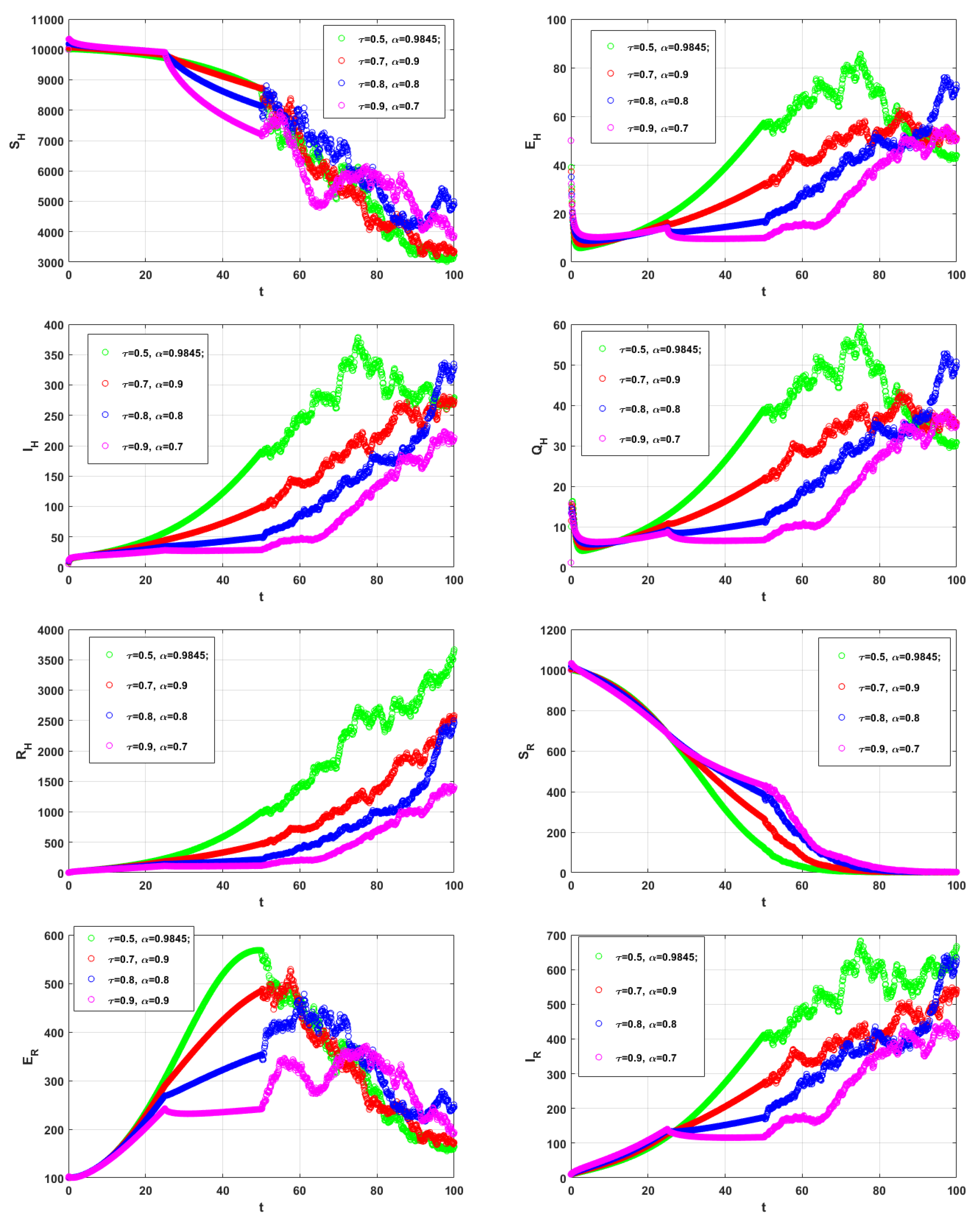
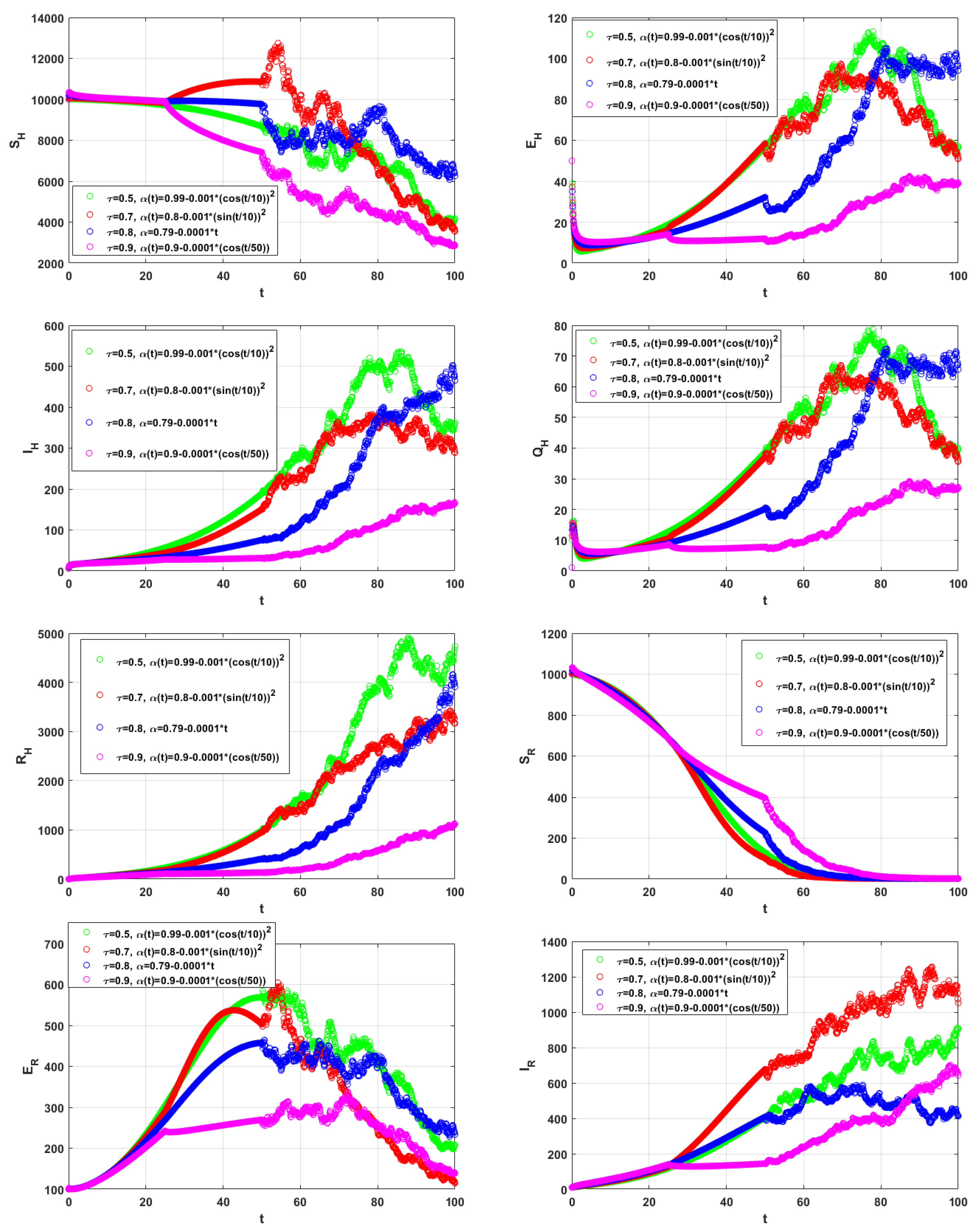
6. Numerical Simulations

In this section, we try to validate the analytical expressions obtained in the previous sections and the reported experimental results. For numerical and computational purposes, we employ the following parameters: $A_H=1/(79\times 365),$ $A_R=0.60822,$ $b_1=0.011503,$ $b_2=0.747322,$ $b_3=0.321102,$ $a_1=0.423890,$ $a_2=1.797575,$ $a_3=0.025289,$ $v=1.575454,$ $u=0.999763,$ $r=0.067689,$ $m_H=1/(79\times 365),$ $m_R=(1/(5\times 365)),$ $d_H=0.015016,$ $d_R=0.000025.$

Real data from the United States were used to estimate and fit the parameter values. These data are available in [2]. Moreover, the initial values are given as follows: ${\mathcal{E}}_{\mathcal{R}}(0)=100,$ ${\mathcal{I}}_{\mathcal{R}}(0)=10,$ ${\mathcal{E}}_{\mathcal{H}}(0)=50,$ ${\mathcal{R}}_{\mathcal{H}}(0)=0,$ ${\mathcal{S}}_{\mathcal{R}}(0)=1000,$ ${\mathcal{I}}_{\mathcal{H}}(0)=5.86,$ ${\mathcal{Q}}_{\mathcal{H}}(0)=1.14,$ ${\mathcal{S}}_{\mathcal{H}}(0)=\mathrm{10,000},$ $T_f=100,$ $t_2=50,$ and $t_1=25.$ Before these points, the dynamics exhibit multiplicity in their behavior. This prompts us to examine and forecast the progression of the disease from its onset to its conclusion, providing the opportunity to observe various behaviors ranging from crossover to stochastic processes. The behavior of the solutions of the piecewise monkeypox model Equations (6)–(11) using CPC-AB5SM (18), (24), and NMEM (25), where $\Theta (\Delta t)=1-e^{-\Delta t}$ with various values of $\alpha ,H^{*},\tau$, and $\alpha (t)$ are shown in Figure 1, Figure 2 and Figure 3.

Figure 4 shows the comparison between the real data from the United States (13 June to 16 September 2022), with a 7-day moving average fitted, and the results we obtained from using the proposed method for the crossover model presented.

Figure 1 illustrates how the solutions of the proposed model change with different values of $H^{*}$, $\alpha =0.9845,$ $\alpha (t)=0.99-0.0001t,$ and $\tau =0.9.$ We noted that the behavior of the crossover system changed after $T_2=50.$

Figure 2 illustrates the behavior of the solution of (6)–(11) for different values of $\tau$ and $\alpha ,$ $H^{*}=0.8,$ $\alpha (t)=0.99-0.0001t.$ We noted that before these points, $T_f=100$, $t_2=50$, and $t_1=25,$ The solutions display diversity in their behavior.

Figure 3 shows the simulation for (6)–(10), and different values of $\tau ,$ $\alpha (t),$ and $\alpha =0.8,$ $H^{*}=0.8.$ We noted that the behavior of the crossover system clearly changed before $t_2=50$ and $T_f=100,$ and did not change before $t_1=25.$ The simulation revealed various deep insights into the model, which was beneficial from both biological and mathematical viewpoints.

7. Conclusions

A novel crossover monkeypox disease model with time delay was developed. Three different models of variable order, fractional order, and fractional stochastic derivatives are defined in three intervals of time. CPC-NAB5SM (17) and NMEMM (25) were constructed to study the behavior of these models with time delay, including Brownian motion into stochastic differential equations, which provided vital insights into the unpredictable nature of disease progression.

Our numerical experiments demonstrate the efficacy of these methods and provide strong empirical support for our theoretical findings. Perhaps most importantly, our findings have opened up new avenues for understanding the monkeypox pandemic.

The concept of piecewise derivatives guides us in analyzing and predicting the evolution of the disease from inception to conclusion, providing the opportunity to observe different behaviors, ranging from crossover to stochastic processes. Additionally, the incorporation of piecewise differential operators constructed with fractional and variable-order operators, such as the CPC operator with stochastic derivatives, has broadened the horizons for readers across different disciplines. These operators enable the capture of various behaviors at different time intervals. Consequently, researchers can effectively model real-world problems by employing this operator, enhancing their understanding of complex phenomena.

References

1. Özköse, F.; Yılmaz, S.; Yavuz, M.; Öztürk, İ.; Şenel, M.T.; Bağcı, B.Ş.; Doğan, M.; Önal, Ö. A Fractional Modeling of Tumor-Immune System Interaction Related to Lung Cancer with Real Data. Eur. Phys. J. Plus. 2022, 137, 40. [Google Scholar] [CrossRef]
2. Peter, O.J.; Kumar, S.; Kumari, N.; Oguntolu, F.A.; Oshinubi, K.; Musa, R. Transmission dynamics of Monkeypox virus: A mathematical modelling approach. Model. Earth Syst. Environ. 2022, 8, 3423–3434. [Google Scholar] [CrossRef] [PubMed]
3. Breman, J.G. Monkeypox: An emerging infection for humans. Emerg. Infect. 2000, 4, 45–67. [Google Scholar]
4. Riopelle, J.C.; Munster, V.J.; Port, J.R. Atypical and unique transmission of monkeypox virus during the 2022 outbreak: An overview of the current state of knowledge. Viruses 2022, 14, 2012. [Google Scholar] [CrossRef]
5. Kumar, N.; Acharya, A.; Gendelman, H.E.; Byrareddy, S.N. The 2022 outbreak and the pathobiology of the monkeypox virus. J. Autoimmun. 2022, 131, 102855. [Google Scholar] [CrossRef]
6. Usman, S.; Adamu, I.I. Modeling the transmission dynamics of the monkeypox virus infection with treatment and vaccination interventions. J. Appl. Math. Phys. 2017, 5, 2335. [Google Scholar] [CrossRef]
7. Khan, A.; Sabbar, Y.; Din, A. Stochastic modeling of the Monkeypox epidemic with cross-infection hypothesis in a highly disturbed environment. Math. Biosci. Eng. 2022, 19, 13560–13581. [Google Scholar] [CrossRef] [PubMed]
8. Grant, R.; Nguyen, L.B.L.; Breban, R. Modelling human-to-human transmission of monkeypox. Bull. World Health Organ. 2020, 98, 638. [Google Scholar] [CrossRef]
9. Bankuru, S.V.; Kossol, S.; Hou, W.; Mahmoudi, P.; Rycht, J.; Taylor, D. A game-theoretic model of Monkeypox to assess vaccination strategies. PeerJ 2020, 8, e9272. [Google Scholar] [CrossRef]
10. Syam, M.I.; Al-Refai, M. Fractional differential equations with Atangana-Baleanu fractional derivative: Analysis and applications. Chaos Solitons Fractals 2019, 2, 100013. [Google Scholar] [CrossRef]
11. Sweilam, N.H.; L-Mekhlafi, S.M.A.; Baleanu, D. A hybrid stochastic fractional order Coronavirus (2019-nCov) mathematical model. Chaos Solitons Fractals 2021, 145, 110762. [Google Scholar] [CrossRef]
12. Agarwal, P.; Baleanu, D.; Chen, Y.-Q.; Momani, S.; Machado, J.A.T. Fractional Calculus; Springer: Singapore, 2019. [Google Scholar]
13. Salahshour, S.; Ahmadian, A.; Senu, N.; Baleanu, D.; Agarwal, P. On analytical solutions of the fractional differential equation with uncertainty: Application to the Basset problem. Entropy 2015, 17, 885–902. [Google Scholar] [CrossRef]
14. Baleanu, D.; Fernandez, A.; Akgül, A. On a fractional operator combining proportional and classical differintegrals. Mathematics 2020, 8, 360. [Google Scholar] [CrossRef]
15. Li, B.; Zhang, T.; Zhang, C. Investigation of financial bubble mathematical model under fractal-fractional Caputo derivative. Fractals 2023, 31, 2350050-31. [Google Scholar] [CrossRef]
16. Li, B.; Eskandari, Z. Dynamical analysis of a discrete-time SIR epidemic model. J. Frankl. Inst. 2023, 360, 7989–8007. [Google Scholar] [CrossRef]
17. Shah, K.; Abdeljawad, T.; Ali, A. Mathematical analysis of the Cauchy type dynamical system under piecewise equations with Caputo fractional derivative. Chaos Solitons Fractals 2022, 161, 112356. [Google Scholar] [CrossRef]
18. Shah, K.; Abdeljawad, T.; Alrabaiah, H. On coupled system of drug therapy via piecewise equations. Fractals 2022, 30, 2240206. [Google Scholar] [CrossRef]
19. Shah, K.; Naz, H.; Abdeljawad, T.; Abdalla, B. Study of fractional order dynamical system of viral infection disease under piecewise derivative. CMES 2023, 136, 921–941. [Google Scholar] [CrossRef]
20. Atangana, A.; Araz, S.İ. New concept in calculus: Piecewise differential and integral operators. Chaos Solitons Fractals 2021, 145, 110638. [Google Scholar] [CrossRef]
21. Atangana, A.; Araz, S.İ. Modeling third waves of COVID-19 spread with piecewise differential and integral operators: Turkey, spain and czechia. Results Phys. 2021, 29, 104694. [Google Scholar] [CrossRef]
22. Sweilam, N.H.; Al-Mekhlafi, S.M.; Hassan, S.M.; Alsenaideh, N.R.; Radwan, A.E. Numerical treatments for some stochastic-deterministic chaotic systems. Results Phys. 2022, 38, 105628. [Google Scholar] [CrossRef]
23. Atangana, A.; Araz, S.İ. Deterministic-Stochastic modeling: A new direction in modeling real world problems with crossover effect. Math. Biosci. Eng. 2022, 19, 3526–3563. [Google Scholar] [PubMed]
24. Atangana, A.; Koca, I. Modeling the spread of Tuberculosis with piecewise differential operators. Comput. Model. Eng. Sci. 2022, 131, 787–814. [Google Scholar] [CrossRef]
25. Zhang, T.; Li, Z. Analysis of COVID-19 epidemic transmission trend based on a time 190 delayed dynamic model. Commun. Pure Appl. Anal. 2021, 22, 1–18. [Google Scholar] [CrossRef]
26. Devipriya, R.; Dhamodharavadhani, S.; Selvi, S. SEIR Model for COVID-19 epidemic using delay differential equation. J. Physics 2021, 1767, 012005. [Google Scholar] [CrossRef]
27. Kiselev, I.N.; Akberdin, I.R.; Kolpakov, F.A. A Delay Differential Equation Approach to Model the COVID-19 Pandemic. medRxiv 2021. [Google Scholar] [CrossRef]
28. Ebraheem, H.K.; Alkhateeb, N.; Badran, H.; Sultan, E. Delayed dynamics of SIR model for 205 COVID-19. OPen J. Model. Simulation 2021, 9, 146–158. [Google Scholar] [CrossRef]
29. Rihan, F.A.; Alsakaji, H.J.; Rajivganthi, C. Stochastic SIRC epidemic model with time-delay for COVID-19. Adv. Differ. Equations 2020, 502, 2020. [Google Scholar] [CrossRef]
30. Nastasi, G.; Perrone, C.; Taffara, S.; Vitanza, G. A time-delayed deterministic model for the spread of COVID-19 with calibration on a real dataset. Mathematics 2022, 10, 661. [Google Scholar] [CrossRef]
31. Khan, A.; Ikram, R.; Din, A.; Humphries, U.W.; Akgul, A. Stochastic COVID-19 SEIQ epidemic model with time-delay. Results Phys. 2021, 30, 104775. [Google Scholar] [CrossRef]
32. Podlubny, I. Fractional Differential Equations; Academic Press: New York, NY, USA, 1999. [Google Scholar]
33. Sweilam, N.H.; Al-Mekhlafi, S.M.; Ajami, T.M. Optimal control of hybrid variable-order fractional coronavirus (2019-nCov) mathematical model; numerical treatments. Ecol. Complexity 2022, 49, 100983. [Google Scholar] [CrossRef]
34. Gómez-Aguilar, J.F.; Rosales-García, J.J.; Bernal-Alvarado, J.J.; Córdova-Fraga, T.; Guzmán-Cabrera, R. Fractional mechanical oscillators. RevisaMex Fis. 2012, 58, 348–352. [Google Scholar]
35. Ullah, M.Z.; Baleanu, D. A new fractional SICA model and numerical method for the transmission of HIV/AIDS. Math Meth. Appl. Sci. 2021, 44, 8648–8659. [Google Scholar] [CrossRef]
36. Mickens, R. Nonstandard Finite Difference Models of Differential Equations; World Scientific: Singapore, 1994. [Google Scholar]
37. Scherer, R.; Kalla, S.; Tang, Y.; Huang, J. The Grünwald-Letnikov method for fractional differential equations. Comput. Math. Appl. 2011, 62, 902–917. [Google Scholar] [CrossRef]
38. Hu, Y.; Liu, Y.; Nualart, D. Modified Euler approximation scheme for stochastic differential equations driven by fractional Brownian motions. arXiv 2013, arXiv:1306.1458vl. [Google Scholar]
Figure 1. Simulation for (6)–(10), and different values of H * ,   α = 0.9845 ,   α ( t ) = 0.99 0.0001 t ,   τ = 0.9   σ 1 = 0.05 ,   σ 2 = 0.04 ,   σ 3 = 0.01 ,   σ 4 = 0.05 ,   σ 5 = 0.04 ,   σ 6 = 0.01 ,   σ 7 = 0.05 ,   σ 8 = 0.04 .
Fractalfract 08 00185 g001
Figure 2. Simulation for (6)–(10), and different values of τ and α ,   H * = 0.8 ,   α ( t ) = 0.99 0.0001 t ,   σ 1 = 0.05 ,   σ 2 = 0.04 ,   σ 3 = 0.01 ,   σ 4 = 0.05 ,   σ 5 = 0.04 ,   σ 6 = 0.01 ,   σ 7 = 0.05 ,   σ 8 = 0.04 .
Fractalfract 08 00185 g002
Figure 3. Simulation for (6)–(10), and different values of τ ,   α ( t ) , and α = 0.8 ,   H * = 0.8 ,   α ( t ) = 0.99 0.0001 t ,   σ 1 = 0.05 ,   σ 2 = 0.04 ,   σ 3 = 0.01 ,   σ 4 = 0.05 ,   σ 5 = 0.04 ,   σ 6 = 0.01 ,   σ 7 = 0.05 ,   σ 8 = 0.04 .
Fractalfract 08 00185 g003
Figure 4. Monkeypox data from the United States (13 June to 16 September 2022), with a 7-day moving average fitted.
Fractalfract 08 00185 g004