Abstract
In this paper, a fractional-order control method based on the twin-delayed deep deterministic policy gradient (TD3) algorithm in reinforcement learning is proposed. A fractional-order disturbance observer is designed to estimate the disturbances, and the radial basis function network is selected to approximate system uncertainties in the system. Then, a fractional-order sliding-mode controller is constructed to control the system, and the parameters of the controller are tuned using the TD3 algorithm, which can optimize the control effect. The results show that the fractional-order control method based on the TD3 algorithm can not only improve the closed-loop system performance under different operating conditions but also enhance the signal tracking capability.
1. Introduction
Fractional-order calculus stands out for its flexible description of the behavior of nonlocal and non-Markovian dynamics, providing a rich mathematical tool for modeling complex systems. Its main applications include the modeling of nonlinear and nonsmooth system dynamics [1], the simulation of multiscale complex systems [2], the analysis of non-Markovian processes [3], as well as in the fields of signal processing, control systems and financial modeling [4]. In the field of control, fractional-order control has been combined with many traditional control schemes, such as fractional-order PID control [5], fractional-order robust control [6], and fractional-order sliding-mode control [7]; these fractional-order control methods have been developed in depth at the theoretical level to form a sound theoretical system and have achieved extensive and powerful results in practical applications.
As a traditional control strategy, fractional-order sliding-mode control is able to cope with the nonlinearity and uncertainty of the system more flexibly [8,9,10]. However, with the increase in system complexity and nonlinearity, choosing the optimal values of controller parameters often becomes a great difficulty [11]. Faced with this problem, different scholars have used a variety of optimization algorithms over the years, such as early adaptive control [12], the particle swarm algorithm [13], the genetic algorithm [14], and the wolf-pack algorithm [15]. These algorithms have had some success, but as technology advances, they struggle to handle increasingly complex problems.
In recent years, with the continuous development of artificial intelligence technology, more and more advanced algorithms have been applied to the control field [16]. Among them, reinforcement learning algorithms based on neural networks are increasingly becoming a focus of research because their flexibility and adaptability make them more adaptable to complex environments [17,18,19,20,21,22,23]. Reinforcement learning efficiently masters system dynamics by learning through the interaction of an agent with the environment [24]. This approach transforms the system control problem into a process in which the agent learns the optimal control strategy through continuous trial and error [25], and it can also learn without prior knowledge of the system model [26,27], which offers a flexible approach for real-time controller parameter optimization. Specifically, under the framework of reinforcement learning, the intelligent body adjusts the control strategy according to feedback signals by interacting with the environment and gradually optimizes the controller parameters [28,29]. This learning approach is more adaptive, especially in the face of a high-order system complexity, significant nonlinearities, and rapid changes in dynamic characteristics, where traditional static parameter optimization methods may appear to be inadequate [30]. Therefore, reinforcement learning provides a more intelligent solution for controller parameter optimization, which is expected to show more significant performance improvements in practical applications.
In this paper, a fractional-order control method based on TD3 reinforcement learning is proposed to optimize the parameters. A fractional-order disturbance observer is designed for estimating the disturbance signals present in the system, while an RBF network is designed for approximating the possible uncertainties in the system, and finally, a fractional-order sliding-mode controller is designed for controlling the system. For the parameter optimization part, it is performed by the TD3 reinforcement learning algorithm, which consists of six deep neural network networks designed to inhibit the bootstrap phenomenon in the reinforcement learning algorithm [31], so that the output of the network can converge to the optimal solution quickly. On this theoretical basis, a valve-controlled hydraulic system is selected for design and simulation in Matlab/Simulink to verify the effectiveness of the method proposed in this paper, and at the same time, in order to reflect the advantages and disadvantages of the proposed method, a series of comparative experiments are designed.
In summary, the main work of this paper can be succinctly summarized in the following three areas:
- i.
- The fractional-order disturbance observer is designed to estimate the system disturbance signal, and the RBF network is selected to approximate the uncertainties of the system; then, a fractional-order sliding-mode controller is designed to control the system according to the estimated value of the disturbance observer;
- ii.
- The TD3 algorithm is introduced to optimize the parameters of the controller, and an improved loss function is designed to improve the learning performance of the algorithm, accelerate the convergence of the network output, and optimize the control effect;
- iii.
- It is verified through simulation that not only the control effect of the proposed method is better than the selected comparison control method, but that its also has a great robustness and generalization capability.
This paper is organized as follows. Section 2 introduces the proposed fractional-order control method, including the system state equation generalization and the designed fractional-order disturbance observer with an RBF network structure, based on which the fractional-order sliding-mode controller is designed. Section 3 introduces the fundamentals of the TD3 algorithm [32] and defines the reward function and loss function used. Section 4 demonstrates the stability of the designed method to verify its theoretical correctness. In Section 5, the proposed method is simulated in Matlab/Simulink using a valve-controlled hydraulic system as a model, and a series of control simulations are performed to verify the practical feasibility of the proposed method. Finally, conclusions and future work are presented.
2. Design of Fractional-Order Control Method
In this section, the fractional-order control part of the proposed method is accomplished for a system generalization including a fractional-order disturbance observer, an RBF network, and a fractional-order sliding-mode controller.
For a common system, the equation of state can be expressed as
where x is the system state, and ; A is the system parameter matrix, , B is the control matrix, and ; u is the control signal, , is the output matrix, is the disturbance signal, and is the uncertainty of system.
In this paper, the Riemann–Liouville fractional-order calculus formula is defined as [33]:
where represents the differential, , represents the Gamma function, n represents the smallest integer larger than , usually taken as 1, and a, x represents the lower and upper limits of the integral.
For the disturbance signal, the fractional-order disturbance observer is given by
where z is the disturbance observer auxiliary vector, L is the gain matrix, is the Hurwitz matrix with n distinct eigenvalues, is the estimate of the disturbance, and is an estimate of the model uncertainty.
Theorem 1.
Assume that the disturbance is bounded and its derivative is also bounded, which means that , . Define the estimation error of the disturbance . Based on the structure of the designed disturbance observer, the estimation error of the disturbance is bounded when the system uncertainty estimation error is bounded, which means that , where ξ is a very small constant greater than zero.
Proof.
Define ; then, M is a Hurwitz matrix with n distinct eigenvalues, so there exists an invertible matrix X such that . Therefore, there exists a positive constant such that , where [34]. Differentiating the estimation error for the disturbance yields the following equation:
It can be obtained that . The subsequent proof is given in the stability analysis on . □
For the model uncertainty that may exist in the system, a radial basis function (RBF) network is used for approximation. The network structure of an RBF has the ability for high-speed learning, the ability to approximate a nonlinear function, which improves the model’s fitting ability, and it can adapt to a variety of complex input–output mapping, so it is very flexible in practical applications. Moreover, compared with other types of neural networks, the RBF network structure is relatively simple, which makes it easy to realize and adjust [35]. The structure of the RBF network used in this paper is shown in Figure 1.
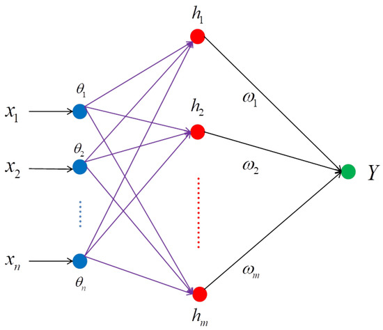
Figure 1.
Structure of the RBF network.
The input–output relationship for each layer can be expressed as an input layer, , an implicit layer, , and an output layer, , where is the Euclidean paradigm, H is an implicit layer function vector , is the center vector, is the width of the radial basis function, and is the ith set of column vectors of the weight matrix W from the implicit layer to the output layer, which means that , where i is the number of neurons in the input and output layer, and j is the number of neurons in the hidden layer.
Defining the optimal weights vector as , the system uncertainty part function can be expressed as [36]
where is the smallest approximation error of the RBF network, , is the arithmetic function from the input layer to the output of the implicit layer; since the system uncertainty is bounded, there exists an upper bound for , which means that .
Defining the estimate of the RBF network for the system uncertainty as , the estimation error can be written as [36]
where satisfies , with a bounded constant.
Based on the fractional-order disturbance observer’s estimate of the disturbance signal and the RBF network’s estimate of the system’s uncertainty , the sliding-mode surface of the fractional-order sliding-mode controller is given by
where e is the system tracking error, , determined by the desired output and the actual output y of the system, and are positive real numbers, and is the order of the fractional-order differentiation.
Deriving the sliding-mode surface and taking the sliding-mode convergence law as , where and k are the sliding-mode convergence law parameters and , and substituting into (1), the control law can be obtained by
Substituting the disturbance signal estimator of (3) with the system uncertainty estimator yields the following final control law:
3. TD3 Algorithm Based on Fractional-Order Control Method
In this section, a TD3 algorithm based on the designed fractional-order control method is proposed, and we design the reward function and loss function of the TD3 algorithm based on the proposed fractional-order control method, which in turn makes it effective for the optimization of the parameters of the fractional-order control method.
As a kind of reinforcement learning algorithm, the basic principle of the TD3 algorithm is also composed of a critic and an actor, two kinds of networks of the agent and the environment for the interactive operation. More specifically, Figure 2 shows the agent interacting with the environment to obtain the state and rewards , the output of the action at moment t, and the update of the two kinds of networks within the agent is based on the loss function.
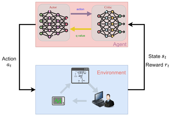
Figure 2.
The relationship between environment and agent.
In this paper, the state of the environment is set as the error signal for each state of the system, which means that , and the reward signal is set to the negative of the weighted sum of the absolute values of the error signals for each state of the system, which means , where denotes the weight of the ith error signal in the reward function, which needs to be set according to the actual situation; the action of the actor network’s output are the parameters of the fractional-order controller which should be optimized.
In the reinforcement learning algorithm, the Bellman equation is defined as [37]
where denotes the reward acquired by the intelligence in the environment, is a value function that represents the sum of the rewards that the intelligence expects to acquire in a continuous process after moment t, and where denotes the discount rate.
For both sides of (9), the expectation based on the state S and action A at a moment can be obtained, and the value function of the action at that moment can be obtained by
In the reinforcement learning algorithm, the estimation of the value function of the action is carried out through the critic network, so there is a certain bias, at which point the Bellman equation’s equal sign does not hold. Defining the difference between the left and right sides of (10) as the temporal-difference error (TD error) , it can be written as [38]
where is the parameter of the critic network at moment t.
In order to solve the bootstrapping of the overestimation in traditional reinforcement learning algorithms, the TD3 algorithm adopts two sets of critic networks and target critic networks with identical structure and parameters; the corresponding network outputs are called Critic1 network , Critic2 network , Target Critic1 network , and Target Critic2 network . The algorithm adopts the strategy of smoothing regularization to reduce the estimation error, adding a noise signal to the action output from the actor network, so that the target value can be expressed as [31]
The agent in the TD3 algorithm stores each state transfer pair in the replay buffer during each interaction with the environment, and since in the process of learning by the intelligent body, the selection of the experience should be considered to prioritize the learning value, in this paper, a nonuniform sampling was designed as
where denotes the probability of drawing a state transfer pair corresponding to reward , is a parameter that controls the shape of the distribution, and n denotes the total number of samples in the replay buffer.
Based on the sampling probability in (13), N samples are taken from the replay buffer and the loss function of the critic network is constructed using the mean squared error (MSE), which can be written as
For the actor network, in order to maximize the future expected return of the current strategy, which means that , and in order to improve the explorability of the action space, the loss function was designed as
where is the parameter of the actor network, is a measure of uncertainty in the distribution of strategies, and is the weight parameter for that item.
For both critic network and actor network parameters , are updated using the gradient descent method, which can be expressed as [31]
where and are the learning rate of the critic network and actor network.
For the target network parameter, a soft update is performed by introducing the update shift of the network parameter, which means [31]:
Finally, the TD3 algorithm uses lagged updating for the actor network, which means that the actor network is updated once when the critic network is updated multiple times. Based on the above description, a structure of a fractional-order control method based on the TD3 algorithm is proposed, and the corresponding pseudocode is shown in Algorithm 1.
| Algorithm 1 FOCS pseudocode based on the TD3 algorithm |
| Initialize critic networks and and actor network with |
| random parameters , , |
| Initialize target networks , , |
| Initialize replay buffer |
| for to do |
| Output action based on current parameters , , |
| Take for FOCS, observe the error , calculate r, and observe new state |
| Store the transfer pair in |
| if n is the number of transfer pair in replay buffer . |
| Sample N transfer pairs and calculate the loss function of critic network |
| Update by |
| if Critic network after d updates |
| Calculate the loss function of critic network |
| Update by |
| Update target network by |
| end if |
| end if |
| end for |
4. Stability Analysis
In this section, the stability of the proposed control method is substantiated through a detailed proof, emphasizing the theoretical feasibility of the proposed approach.
For the proposed fractional-order disturbance observer, the Lyapunov function is defined as
The derivation of (18) and substitution into (1), (3), and (5) yield
where is the largest eigenvalue of M which is a Hurwitz matrix so it can be obtained that . In order to make the estimation error of the fractional-order disturbance observer for the disturbance signal stable, M should satisfy .
In order to keep the approximation error of the designed RBF network for the system uncertainty within a certain range, the adaptive law of the RBF network weights and the implicit layer function update law are taken as
where is the designed positive-definite diagonal matrix, are the designed parameters of the adaptive law, s and are the sliding-mode surface and the parameter which was designed in (6), and H is the implicit layer function vector.
For the proposed RBF network, the Lyapunov function is defined as
Based on the designed sliding-mode surface function, define the Lyapunov function
Deriving equation (23) and substituting the system state equation shown in (1) with the control law shown in (8) yield
To prove the overall stability of the original system with the addition of a fractional-order control method, define the Lyapunov function
5. Simulation Result
In this section, in order to validate the effectiveness of the proposed methodology, a valve-controlled hydraulic system is selected as the object of study to design a series of simulations. Firstly, to verify the online learnability of the TD3 algorithm, three rounds of training states during the training process are selected for the comparison. Secondly, the control effect is verified for the optimized fractional-order control method of the TD3 algorithm by employing the prescribed performance fractional-order sliding-mode controller (PPC-FOSMC), an unoptimized fractional-order sliding-mode controller (FOSMC), and a sliding-mode controller (SMC). Furthermore, the antidisturbance is proved for the proposed method, and the simulation verification is carried out for different input signals and disturbance signals. The results show that the fractional-order control method based on the TD3 algorithm not only has good online learning ability and generalization ability but also has a better control effect than the traditional FOSMC, SMC, and PPC-FOSM. Finally, in order to verify that the designed method can still maintain a better control effect under noise disturbance, a Gaussian noise is selected as the disturbance signal to simulate using the online learning method.
5.1. Simulation Results of System Online Learning
A valve-controlled hydraulic system is a third-order system [39] which can be described approximately as
where denotes the position, velocity, and acceleration, respectively, u denotes the control input, and y denotes the output of the position. The state matrix, input matrix, disturbance matrix, and output matrix , and C are, respectively,
where , , , , and the values of the parameters of the valve-controlled hydraulic system are shown in Table 1.

Table 1.
Parameters of the valve-controlled hydraulic system.
The disturbance signal during the TD3 training was set to be , the system uncertainty was , and the system expected the output position signal to be ; the training parameters are shown in Table 2.

Table 2.
Parameters of the TD3 algorithm.
Learning to train the system with the above parameters, the episode rewards and average rewards obtained after 1900 episodes are shown in Figure 3a, and Figure 3b–d show the state of the system for the selected episode 1, episode 500, and episode 1826. It can be noticed that in the first 420 episodes, the episode reward fluctuates a lot, and after episode 420, the episode reward and the average reward stabilize for the first time, but at that point, the network still cannot achieve a particularly good training effect. From episode 630 to episode 1300, the agent further explores the action space, and after episode 1300, the episode reward and average reward converge to more optimal values, corresponding to the system state. It can be found that the position and velocity signals of the system corresponding to episode 1 have the worst tracking performance with both large errors and desired signals, while the acceleration signals have the worst tracking performance with more noise. Compared to episode 1, episode 500’s systematic position signal can already track the desired signal at the 0.8th second but with a small error, the velocity signal can track the desired signal after 2 s but with a small noise in between, and the acceleration signal can only track the desired signal after the 4th second. Finally, compared to the previous two, episode 1826 is definitely the best performer, with the position signal tracking the desired signal in the first 0.1 s with very little error, and the velocity signal tracking the desired signal with little error after that, despite oscillating in the first 0.1 s, and with the acceleration signal tracking the desired signal after oscillating in the first 0.4 s with an acceptable error.
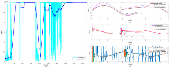
Figure 3.
Episode reward and average reward with the training results of the 1826th episode: (a) episode reward and average reward of 1900 episodes, (b) the 1st, 500th, and 1826th episode’s position and expected position signals; (c) the 1st, 500th, and 1826th episode’s speed and expected signals; (d) the 1st, 500th, 1826th episode’s acceleration and expected signals.
In order to better visually represent the training state of set 1826, the system’s individual signals and desired signals and their errors at that point in time are shown in Figure 4. It can be seen that the position, velocity, and acceleration signals of the system have good tracking performance, and the errors are all within a small range. The same is true for the estimation of disturbance signals.
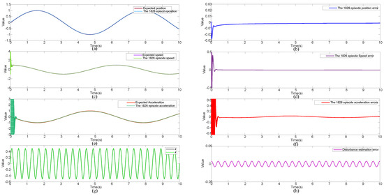
Figure 4.
The 1st, 500th, and 1826th episode’s system signal and expected signals with the error: (a) position signal and expected signal, (b) position tracking error, (c) speed signal and expected signal, (d) speed tracking error, (e) acceleration signal and expected signal, (f) acceleration tracking error, (g) estimation of the disturbance signal and the actual signal, (h) estimation error of the disturbance signal.
5.2. Simulation Results of TD3-FOCS
For the online learning results of the valve-controlled hydraulic fractional-order control method, the training results of the 1826th episode are shown in Figure 5 with , , selected as the controller parameters, and the parameters of FODOB and the RBF network were set to , , and , which is a single-unit diagonal matrix for the subsequent comparative simulation experiments; the simulation time was set to 100 s, and the final results are shown in Figure 6.
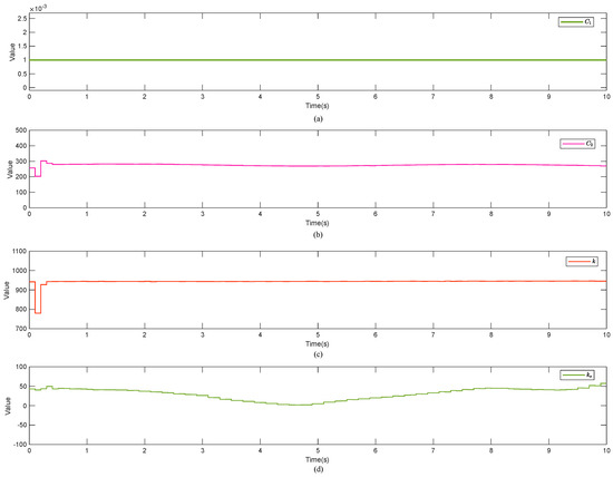
Figure 5.
Training results of the 1826th episode: (a) parameter , (b) parameter , (c) parameter k, (d) parameter .
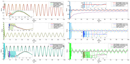
Figure 6.
TD3-optimized fractional-order control vs. unoptimized control method’s system signals and expected signals and their errors: (a) position signal and expected signal, (b) position tracking error, (c) speed signal and expected signal, (d) speed tracking error, (e) acceleration signal and expected signal, (f) acceleration tracking error.
As can be seen from Figure 6, for the position signal, the proposed TD3-FOSMC had the fastest convergence speed (first 0.03 s) and maintained the final steady-state error in the range of (−0.001, +0.001), which was the best among the experimental results. For the velocity signal, it also had the fastest convergence speed (first 0.25 s) and maintained the final steady-state error in the range of , which was the best performance among all the experimental methods. For acceleration signals, although the prescribed performance of the fractional-order sliding-mode controller ended up with a smaller error range, the convergence time was greater than the proposed TD3-FOSMC, which converged in the first 0.3 s. Combining all the above control effects, it can be concluded that the proposed TD3-FOSMC has a better speed and stability.
5.3. Simulation Results of Different Control Signals and Disturbance Signals
In order to demonstrate the robustness and versatility of the method, two control signals (a triangular wave composite signal and a step signal) and two disturbance signals (a strong sine wave signal disturbance and a triangular wave composite signal) were selected for the simulation verification. This allowed a more comprehensive assessment of the method’s antidisturbance performance under different control and disturbance conditions, thus demonstrating the effectiveness of the method in mitigating the effects of an external disturbance in a variety of practical situations.
As observed in Figure 7, the simulation results revealed the capability of accurately tracking the desired signal under the influence of a triangular wave composite signal and a strong sine wave signal disturbance. Specifically, the position signal achieved tracking within a remarkably short duration of 0.07 s, with very small overshoots (less than 1%) in the first 0.02 s, and the final steady-state error confined to a narrow range of (−0.001, 0.001). In the first 0.3 s, the velocity signal had large to small fluctuations in the range of (−3.7, 6); after that, it achieved synchronization with the desired signal and kept the steady-state error within the range of (−0.01, 0.01). On the other hand, the acceleration signal fluctuated in the range of (−12, 12) for the first 0.5 s and was after synchronized with the desired signal and kept the steady-state error within the range of (−0.25, 0.25). The results show that despite the large overshoot in the system response for the different input signals and disturbance signals, the system still had good stability and fast performance.
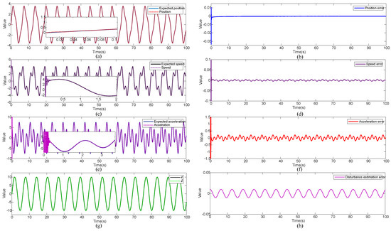
Figure 7.
Simulation results of triangular wave composite signals and strongly interfering sine wave signals: (a) position signal and expected signal, (b) position tracking error, (c) speed signal and expected signal, (d) speed tracking error, (e) acceleration signal and expected signal, (f) acceleration tracking error, (g) estimation of the disturbance signal and actual signal, (h) estimation error of the disturbance signal.
Analyzing the results shown in Figure 8, when subjected to a step signal and a strong triangular wave composite signal disturbance during the simulation, the obtained results exhibited a marginally reduced performance compared to the previous scenario. Taking the simulation time of 10 s as an example, it can be found that for the position, velocity, and acceleration signals, there were large fluctuations in the first 1 s, and their stabilization time was slowing down sequentially. For the position signal, there were fluctuations within the range of (5, 15) within the first 0.3 s; after that, it could track the desired signal, and the final steady-state error was limited to the range of (0, 0.004). The velocity signal exhibited fluctuations within the range of (−10, 10) during the first 0.5 s, after which it synchronized with the desired signal, and the final steady-state error was constrained to (−0.002, 0). For the acceleration signal, fluctuations within the range of (−20, 20) occurred during the initial 0.8 s, following which it converged to the desired value. The final steady-state error remained confined to a smaller range of (−0.0001, 0.0001). Despite a slight decrease in performance, the results underscore the method’s ability to maintain effective control even in the presence of challenging input signals and disturbance conditions.
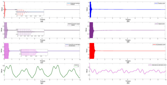
Figure 8.
Simulation results of step signals and triangular wave composite signal: (a) position signal and expected signal, (b) position tracking error, (c) speed signal and expected signal, (d) speed tracking error, (e) acceleration signal and expected signal, (f) acceleration tracking error, (g) estimation of the disturbance signal and actual signal, (h) estimation error of the disturbance signal.
5.4. Simulation Results under Noise Disturbance
The control performance is illustrated for the method under noise disturbance. The noise disturbance signal was selected with a mean value of zero, a variance of five, and a frequency of 10 Hz, and the simulation verification was carried out by using the online learning of the agent. The results are shown in Figure 9.
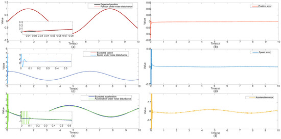
Figure 9.
Simulation results under noise disturbance: (a) position signal and expected signal, (b) position tracking error, (c) speed signal and expected signal, (d) speed tracking error, (e) acceleration signal and expected signal, (f) acceleration tracking error.
Analyzing Figure 9, it can be seen that the position signal exhibited minimal susceptibility form the noise disturbance signal, with an overshoot of less than 3% observed only within the initial 0.03 s. Subsequently, the position signal could track the desired signal, and the final steady-state error could be maintained within the range of (−0.001, 0). The velocity signal demonstrated minimal susceptibility to noise disturbances, with oscillations confined to the range of (−1.6, 4.7) within the initial 0.08 s. Following that period, the signal could adeptly track the desired trajectory, and the final steady-state error could satisfy the narrow bounds of (−0.0015, 0.0015). Comparing with the earlier online learning outcomes, the performance of the acceleration signal was degraded under the noise signal. The acceleration signal was oscillatory within the range of (−6, 6) during the initial 0.15 s. Despite these challenges, it could approximately track the desired signal. However, due to the influence of noise, it maintained a final steady-state error within the range of (−0.13, 0.13). Thus, based on the analysis above, the proposed control method could achieve the control of system within the bounded range under the noise signal.
6. Conclusions
In this paper, a fractional-order control method based on the TD3 algorithm was introduced. A fractional-order disturbance observer was designed to estimate the system’s disturbance signal, and an RBF network was selected to approximate the uncertainties in the system, and the fractional-order sliding-mode control method was also adopted to design the controller. A valve-controlled hydraulic system was simulated and validated in Matlab/Simulink using the agent online learning and the optimization parameters. Different control signals and disturbance signals were used in the optimized fractional-order control system. The results showed that the limitations of this method mainly lay in the difficulty of setting up the training environment comprehensively. Despite some shortcomings, the proposed method was generally fast and had good antidisturbance ability.
Author Contributions
Conceptualization, G.J. and S.S.; methodology, G.J. and Z.A.; software, G.J. and D.S.; validation, G.J. and D.S.; formal analysis, G.J. and Z.A.; writing—original draft preparation, G.J.; writing—review and editing, G.J. and S.S.; supervision, S.S.; funding acquisition, S.S. All authors have read and agreed to the published version of the manuscript.
Funding
This research was funded by the Fund of Science and Technology on Space Intelligent Control Laboratory Foundation (grant number HTKJ2023KL502002); the China Postdoctoral Science Foundation (grant number 2020M681587); the Jiangsu Province Postdoctoral Science Foundation (grant number 2020Z112).
Data Availability Statement
Data are contained within the article.
Conflicts of Interest
The authors declare no conflicts of interest.
References
- Spanos, P.D.; Malara, G. Nonlinear vibrations of beams and plates with fractional derivative elements subject to combined harmonic and random excitations. Probabilistic Eng. Mech. 2020, 59, 142–149. [Google Scholar] [CrossRef]
- Magin, R.L. Fractional calculus models of complex dynamics in biological tissues. Comput. Math. Appl. 2010, 36, 1586–1593. [Google Scholar] [CrossRef]
- Atangana, A. Non validity of index law in fractional calculus: A fractional differential operator with Markovian and non-Markovian properties. Phys. A Stat. Mech. Its Appl. 2018, 505, 688–706. [Google Scholar] [CrossRef]
- Gonzalez, E.A.; Petráš, I. Advances in fractional calculus: Control and signal processing applications. In Proceedings of the 2015 16th International Carpathian Control Conference (ICCC), Szilvasvarad, Hungary, 27–30 May 2015; pp. 147–152. [Google Scholar] [CrossRef]
- Warrier, P.; Shah, P. Optimal Fractional PID Controller for Buck Converter Using Cohort Intelligent Algorithm. Appl. Syst. Innov. 2021, 4, 50. [Google Scholar] [CrossRef]
- Razzaghian, A. A fuzzy neural network-based fractional-order Lyapunov-based robust control strategy for exoskeleton robots: Application in upper-limb rehabilitation. Math. Comput. Simul. 2022, 193, 567–583. [Google Scholar] [CrossRef]
- Fei, J.; Wang, Z.; Pan, Q. Self-Constructing Fuzzy Neural Fractional-Order Sliding Mode Control of Active Power Filter. IEEE Trans. Neural Netw. Learn. Syst. 2023, 34, 10600–10611. [Google Scholar] [CrossRef]
- Jakovljević, B.; Pisano, A.; Rapaić, M.R.; Usai, E. On the sliding-mode control of fractional-order nonlinear uncertain dynamics. Int. J. Robust Nonlinear Control 2016, 24, 782–798. [Google Scholar] [CrossRef]
- Mirrezapour, S.Z.; Zare, A.; Hallaji, M. A new fractional sliding mode controller based on nonlinear fractional-order proportional integral derivative controller structure to synchronize fractional-order chaotic systems with uncertainty and disturbances. J. Vib. Control 2022, 28, 773–785. [Google Scholar] [CrossRef]
- Deepika, D. Hyperbolic uncertainty estimator based fractional-order sliding mode control framework for uncertain fractional-order chaos stabilization and synchronization. ISA Trans. 2022, 123, 76–86. [Google Scholar] [CrossRef] [PubMed]
- Delavari, H.; Ghaderi, R.; Ranjbar, A.; Momani, S. Fuzzy fractional-order sliding mode controller for nonlinear systems. Commun. Nonlinear Sci. Numer. Simul. 2010, 15, 963–978. [Google Scholar] [CrossRef]
- Sun, G.; Ma, Z. Practical tracking control of linear motor with adaptive fractional-order terminal sliding mode control. IEEE/ASME Trans. Mechatron. 2017, 22, 2643–2653. [Google Scholar] [CrossRef]
- Djari, A.; Bouden, T.; Boulkroune, A. Design of fractional-order sliding mode controller (FSMC) for a class of fractional-order non-linear commensurate systems using a particle swarm optimization (PSO) Algorithm. J. Control Eng. Appl. Inform. 2014, 16, 46–55. [Google Scholar]
- Karthikeyan, A.; Rajagopal, K. Chaos control in fractional-order smart grid with adaptive sliding mode control and genetically optimized PID control and its FPGA implementation. Complexity 2017, 2017, 3815146. [Google Scholar] [CrossRef]
- Han, S. Modified grey-wolf algorithm optimized fractional-order sliding mode control for unknown manipulators with a fractional-order disturbance observer. IEEE Access 2020, 8, 18337–18349. [Google Scholar] [CrossRef]
- Salman, G.A.; Jafar, A.S.; Ismael, A.I. Application of artificial intelligence techniques for LFC and AVR systems using PID controller. Int. J. Power Electron. Drive Syst. 2019, 10, 1694. [Google Scholar] [CrossRef]
- Perrusquía, A.; Yu, W. Identification and optimal control of nonlinear systems using recurrent neural networks and reinforcement learning: An overview. Neurocomputing 2021, 438, 145–154. [Google Scholar] [CrossRef]
- Liu, Y.J.; Zhao, W.; Liu, L.; Li, D.; Tong, S.; Chen, C.P. Adaptive neural network control for a class of nonlinear systems with function constraints on states. IEEE Trans. Neural Netw. Learn. Syst. 2023, 34, 2732–2741. [Google Scholar] [CrossRef] [PubMed]
- Chen, Z.; Niu, B.; Zhang, L.; Zhao, J.; Ahmad, A.M.; Alassafi, M.O. Command filtering-based adaptive neural network control for uncertain switched nonlinear systems using event-triggered communication. Int. J. Robust Nonlinear Control 2022, 32, 6507–6522. [Google Scholar] [CrossRef]
- Katz, S.M.; Corso, A.L.; Strong, C.A.; Kochenderfer, M.J. Verification of image-based neural network controllers using generative models. J. Aerosp. Inf. Syst. 2022, 19, 574–584. [Google Scholar] [CrossRef]
- Kiumarsi, B.; Vamvoudakis, K.G.; Modares, H.; Lewis, F.L. Optimal and autonomous control using reinforcement learning: A survey. IEEE Trans. Neural Netw. Learn. Syst. 2017, 29, 2042–2062. [Google Scholar] [CrossRef]
- Duraisamy, P.; Nagarajan Santhanakrishnan, M.; Rengarajan, A. Design of deep reinforcement learning controller through data-assisted model for robotic fish speed tracking. J. Bionic Eng. 2023, 20, 953–966. [Google Scholar] [CrossRef]
- Wei, C.; Xiong, Y.; Chen, Q.; Xu, D. On adaptive attitude tracking control of spacecraft: A reinforcement learning based gain tuning way with guaranteed performance. Adv. Space Res. 2023, 71, 4534–4548. [Google Scholar] [CrossRef]
- Barto, A.G. Reinforcement learning. In Neural Systems for Control; Academic Press: Cambridge, MA, USA, 1997; pp. 7–30. [Google Scholar]
- Nian, R.; Liu, J.; Huang, B. A review on reinforcement learning: Introduction and applications in industrial process control. Comput. Chem. Eng. 2020, 139, 106886. [Google Scholar] [CrossRef]
- Zhu, Y.; Zhao, D.; Li, X. Using reinforcement learning techniques to solve continuous-time non-linear optimal tracking problem without system dynamics. IET Control Theory Appl. 2016, 10, 1339–1347. [Google Scholar] [CrossRef]
- Syafiie, S.; Tadeo, F.; Martinez, E. Model-free learning control of neutralization processes using reinforcement learning. Eng. Appl. Artif. Intell. 2007, 20, 767–782. [Google Scholar] [CrossRef]
- Dogru, O.; Velswamy, K.; Ibrahim, F.; Wu, Y.; Sundaramoorthy, A.S.; Huang, B.; Xu, S.; Nixon, M.; Bell, N. Reinforcement learning approach to autonomous PID tuning. Comput. Chem. Eng. 2022, 161, 107760. [Google Scholar] [CrossRef]
- Taherian, S.; Kuutti, S.; Visca, M.; Fallah, S. Self-adaptive torque vectoring controller using reinforcement learning. In Proceedings of the 2021 IEEE International Intelligent Transportation Systems Conference (ITSC), Indianapolis, IN, USA, 19–22 September 2021; IEEE: Piscataway, NJ, USA, 2021; pp. 172–179. [Google Scholar]
- Yan, L.; Webber, J.L.; Mehbodniya, A.; Moorthy, B.; Sivamani, S.; Nazir, S.; Shabaz, M. Distributed optimization of heterogeneous UAV cluster PID controller based on machine learning. Comput. Electr. Eng. 2022, 101, 108059. [Google Scholar] [CrossRef]
- Wu, J.; Wu, Q.J.; Chen, S.; Pourpanah, F.; Huang, D. A-TD3: An Adaptive Asynchronous Twin Delayed Deep Deterministic for Continuous Action Spaces. IEEE Access 2022, 10, 128077–128089. [Google Scholar] [CrossRef]
- Dankwa, S.; Zheng, W. Twin-delayed ddpg: A deep reinforcement learning technique to model a continuous movement of an intelligent robot agent. In Proceedings of the 3rd International Conference on Vision, Image and Signal Processing, Vancouver, BC, Canada, 26–28 August 2019; pp. 1–5. [Google Scholar]
- Li, C.; Qian, D.; Chen, Y.Q. On Riemann-Liouville and caputo derivatives. Discret. Dyn. Nat. Soc. 2011, 2011, 562494. [Google Scholar] [CrossRef]
- Walsh, G.C.; Ye, H.; Bushnell, L.G. Stability analysis of networked control systems. IEEETrans. Control Syst. Technol. 2002, 10, 438–446. [Google Scholar] [CrossRef]
- Er, M.J.; Wu, S.; Lu, J.; Toh, H.L. Face recognition with radial basis function (RBF) neural networks. IEEE Trans. Neural Netw. 2002, 13, 697–710. [Google Scholar] [PubMed]
- Fei, J.; Wang, H.; Fang, Y. Novel neural network fractional-order sliding-mode control with application to active power filter. IEEE Trans. Syst. Man, Cybern. Syst. 2021, 52, 3508–3518. [Google Scholar] [CrossRef]
- Fei, Y.; Yang, Z.; Chen, Y.; Wang, Z. Exponential bellman equation and improved regret bounds for risk-sensitive reinforcement learning. Adv. Neural Inf. Process. Syst. 2021, 34, 20436–20446. [Google Scholar]
- Doya, K. Reinforcement learning in continuous time and space. Neural Comput. 2000, 12, 219–245. [Google Scholar] [CrossRef]
- Duan, Z.; Sun, C.; Li, J.; Tan, Y. Research on servo valve-controlled hydraulic motor system based on active disturbance rejection control. Meas. Control. 2024, 57, 113–123. [Google Scholar] [CrossRef]
Disclaimer/Publisher’s Note: The statements, opinions and data contained in all publications are solely those of the individual author(s) and contributor(s) and not of MDPI and/or the editor(s). MDPI and/or the editor(s) disclaim responsibility for any injury to people or property resulting from any ideas, methods, instructions or products referred to in the content. |
© 2024 by the authors. Licensee MDPI, Basel, Switzerland. This article is an open access article distributed under the terms and conditions of the Creative Commons Attribution (CC BY) license (https://creativecommons.org/licenses/by/4.0/).