Article

An Efficient Cubic B-Spline Technique for Solving the Time Fractional Coupled Viscous Burgers Equation

1
Department of Mathematics, University of Sargodha, Sargodha 40100, Pakistan
2
Center of Excellence in Theoretical and Computational Science (TaCS-CoS), Faculty of Science, King Mongkut’s University of Technology Thonburi (KMUTT), 126 Pracha-Uthit Road, Bang Mod, Thung Khru, Bangkok 10140, Thailand
3
Department of Physics, College of Science, Taibah University, Al-Madinah Al-Munawarah 41477, Saudi Arabia
4
Theoretical Physics Group, Faculty of Science, Mansoura University, Mansoura 35516, Egypt
5
Department of Mathematics, College of Science, Taibah University, Al-Madinah Al-Munawarah 41477, Saudi Arabia
6
Department of Mathematics, Faculty of Science, Mansoura University, Mansoura 35516, Egypt
*
Author to whom correspondence should be addressed.
Fractal Fract. 2024, 8(2), 93; https://doi.org/10.3390/fractalfract8020093
Submission received: 7 September 2023 / Revised: 8 January 2024 / Accepted: 20 January 2024 / Published: 31 January 2024

Abstract

:
The second order Burger’s equation model is used to study the turbulent fluids, suspensions, shock waves, and the propagation of shallow water waves. In the present research, we investigate a numerical solution to the time fractional coupled-Burgers equation (TFCBE) using Crank–Nicolson and the cubic B-spline (CBS) approaches. The time derivative is addressed using Caputo’s formula, while the CBS technique with the help of a θ -weighted scheme is utilized to discretize the first- and second-order spatial derivatives. The quasi-linearization technique is used to linearize the non-linear terms. The suggested scheme demonstrates unconditionally stable. Some numerical tests are utilized to evaluate the accuracy and feasibility of the current technique.

1. Introduction

The second order viscous Coupled Burgers equations (VCBEs) are considered for numerical solution in this article. This model is used to study physical phenomena such as turbulent fluids, fluid suspensions, shock waves, arising in gas dynamics, the propagation of shallow water waves, continuous stochastic processes, flow theory, and chromatography [1,2,3,4,5]. The non-linear VCBEs are defined as follows:
U t ( x , t ) U x x ( x , t ) + α 1 ( U ( x , t ) V ( x , t ) ) x + γ U ( x , t ) U x ( x , t ) = 0 , a x b , t [ 0 , T ] , V t ( x , t ) V x x ( x , t ) + α 2 ( V ( x , t ) U ( x , t ) ) x + γ V ( x , t ) V x ( x , t ) = 0 , a x b , t [ 0 , T ] ,
with initial conditions (ICs)
U ( x , 0 ) = ϕ 1 ( x ) , V ( x , 0 ) = ϕ 2 ( x ) , a x b
and boundary conditions (BCs)
U ( a , t ) = φ 1 ( t ) , V ( a , t ) = ψ 1 ( t ) , U ( b , t ) = φ 2 ( t ) , V ( b , t ) = ψ 2 ( t ) , t [ 0 , T ]
where α 1 and α 2 are system parameters, which represent the diffusion and interaction of two fluids, respectively, and γ is a constant.
Fractional calculus involves the study of non-integer order derivatives and integrals [6,7,8]. The nonlinear TFCBE with different parameters is defined as follows:
λ U ( x , t ) t λ 2 U ( x , t ) x 2 + α 1 ( U ( x , t ) V ( x , t ) ) x + γ U ( x , t ) U ( x , t ) x = Q 1 , λ V ( x , t ) t λ 2 V ( x , t ) x 2 + α 2 ( U ( x , t ) V ( x , t ) ) x + γ V ( x , t ) V ( x , t ) x = Q 2 , x [ a , b ] , t [ 0 , T ] , λ ( 0 , 1 ) ,
with ICs:
U ( x , 0 ) = ϕ 1 ( x ) , V ( x , 0 ) = ϕ 2 ( x ) ,
the BCs:
U ( a , t ) = φ 1 ( t ) , U ( b , t ) = φ 2 ( t ) , V ( a , t ) = ψ 1 ( t ) , V ( b , t ) = ψ 2 ( t ) ,
where λ is the fractional parameter, λ U ( x , t ) t λ is the time fractional derivative (FD) in the Caputo sense, and U ( x , t ) x = U x ( x , t ) and 2 U ( x , t ) t 2 = U x x ( x , t ) are first- and second-order spatial derivatives, respectively. This model represents the time fractional coupled-Burgers equation (TFCBE) in Caputo’s sense that satisfies the mathematical model accurately and represents the real-world system. These equations are well defined and capture the memory in time direction. The velocity profiles of two distinct fluids are denoted as U ( x , t ) and V ( x , t ) . There are numerous methods to deal with the FD. Usually, the Caputo FD is used to acquire the appropriate real world physical models. In this paper, Caputo’s FD of the function is employed to discretize the temporal derivative. The Caputo FD of the function U ( x , t ) with order λ ( 0 , 1 ) is given as follows:
λ U ( x , t ) t λ = 1 Γ ( 1 λ ) 0 t U ( x , κ ) κ d κ ( t κ ) λ , 0 < λ < 1 , U ( x , t ) t , λ = 1 ,
where the Euler’s Gamma function is represented by Γ .
Numerous approaches have been developed to deal with the initial and boundary value problems. Chen et al. [9] represented an approximate solution to coupled Burgers equations (CBEs) with FD using the Adomian decomposition method (ADM). Khan et al. [10] studied the Burgers and a system of Burgers equations using the homotopy perturbation method (HPM). They also solved these problems using a generalized differential transform method (GDTM) involving the Caputo time FD. CBEs have been solved by Prakash et al. [11] via a time fractional variational iteration approach. They compared their results with other methods, namely the HPM, the ADM, and the generalized differential transformation method (GDTM). The CBEs have also been solved using the q-homotopy analysis transform method by Singh et al. [12]. Aminikhah and Malekzadeh [13] developed a new HPM, in order to calculate the system of the CBEs and temporal FD that is used with the Caputo formula. In [14], a reduced differential transform method, the Laplace ADM, and the Laplace-variational iteration scheme have been utilized to investigate a solution to the CBEs. Albuohimad and Adibi proposed a solution to the CBEs using the hybrid spectral exponential Chebyshev method (HSECM), and the FD derivative was discretized utilizing the finite difference method (FDM) [15]. Sulaiman investigated the system of viscous Burgers equations using the Atangana–Baleanu FD to obtain a numerical simulation in [16]. A system Burgers equation was estimated using the generalized differential transform method (DTM) and the Caputo derivative (CD), employed to solve the temporal FD in [17]. Ozdemir et al. [18] calculated approximate solutions to Burgers equations by proposing Gegenbauer wavelets-based computational methods with TFD. Abazari and Borhanifar [19] developed an approximate solution to the CBEs through a differential transformation method. They also compared their approximate results with three different methods, namely the variational iteration, HPM, and analysis techniques. Mittal and Arora [20] investigated a system of viscous Burgers equations, discretized the scheme using the CBS collocation, and investigated the stability of the scheme. Shukla et al. [21] used a modified CBS to study the two-dimensional nonlinear VCBEs and found approximate solutions using the differential quadrature method. Kumar and Arora [22] employed approximate solutions to the coupled Klein Gordon equation and a system of Burgers equations through a reduced differential transformation scheme. Srivastava et al. [23] used the implication logarithmic FDM to present an approximation of a solution to the nonlinear CBEs. Mittal and Tripathi [24] investigated an approximate solution to a system of Burgers equation with the help of a modified spline. Sarboland and Aminataei [25] solved the nonlinear CBEs through a multiquadric quasi-interpolation scheme. Salih et al. [26] proposed a numerical solution to CBEs with Dirichlet’s boundary conditions by using trigonometric spline functions. He and Tang [27] developed a lattice Boltzmann to find a numerical solution to CBEs. Chuathong and Kaennakham [28] suggested a collocation method to determine approximate solutions to CBEs. Jima et al. [29] presented an approximated solution using a differential quadrature method. In [30], the authors presented a Chebyshev wavelets method to investigate a CBE. Guo-Cheng et al. [31] discussed the concept of short memory fractional differential equations with impulses and provided exact solutions for linear cases. Dubey et al. [32] presented a computational algorithm called a local fractional natural homotopy analysis method to solve local fractional coupled Helmholtz and CBEs in fractal media. They also discussed the uniqueness, convergence, and error analysis of the solutions obtained using the method. Numerical simulations on the Cantor set validate the effectiveness of the proposed method. WANG [33] proposed a new fractal modified equal width-Burgers equation (MEWBE) with the local fractional derivative using a Mittag–Leffler function.
Spline interpolation is a valuable method for approximating mathematical functions with a piecewise smooth curve. Specifically, B-spline interpolation utilizes a type of piecewise polynomial that exhibits high localization. There is no study on the implementation of cubic B-spline for the TFCBEs. Inspired by the success of the spline in the numerical solution to integer-order differential equations and fractional order differential equations, the main aim of this study is to investigate the numerical solution to TFCBEs by using cubic B-spline functions. They have been employed by several researchers for solving fractional partial differential equations. The novelty of the proposed work is to discretize the first-order time fractional derivative in the Caputo sense with a first-order Crank–Nicholson finite difference scheme, while the CBS functions are used to discretize the spatial derivatives for coupled equations. It can be easily seen that the work done in this paper provides a more accurate numerical solution to the proposed problem because we use a combination of a Crank–Nicholson finite difference scheme and CBS functions with the help of a θ -weighted scheme. This first-order time fractional derivative discretization in the Caputo sense for coupled equations has never been used, as far as we are aware, for the case of first-order TFCBEs. The superiority of the proposed method is to provide a numerical solution in a piecewise cubic function with the smoothness of C 2 continuity at each joint point of solution.
The paper is structured as follows: Section 2 describes the CBS functions at different knots. Section 3 and Section 4 present the discretization of the fractional derivative and the procedure of the proposed numerical technique, respectively. Section 5 discusses the stability of the suggested technique. The conclusion of the study is presented in Section 6.

2. B-Spline Approximation

Let a = x 0 < x 1 . . . x N 1 < x N = b be the spatial domain on the interval [ a , b ] . In the present section, cubic B-spline approximation for U ( x , t ) and V ( x , t ) is constructed. We define the partition into equivalent sub-intervals of length h = b a N , where x i = a + i h , where i = 0 , 1 , 2 , 3 , . . . , N . The cubic B-spline can be defined as follows:
B i ( x ) = 1 6 h 3 ( x x i 2 ) 3 , x [ x i 2 , x i 1 ] , h 3 3 ( x x i 1 ) 3 + 3 h ( x x i 1 ) 2 + 3 h 2 ( x x i 1 ) , x [ x i 1 , x i ] , h 3 3 ( x i + 1 x ) 3 + 3 h ( x i + 1 x ) 2 + 3 h 2 ( x i + 1 x ) , x [ x i , x i + 1 ] , ( x i + 2 x ) 3 , x [ x i + 1 , x i + 2 ] , 0 , Otherwise .
The B-spline { B 1 , B 0 , . . . , B N , B N + 1 } establishes a basis over the assumed domain. The values of B i ( x ) at the different knots are given in Table 1.
The solution to Equation (4) is considered a linear combination of the CBS by joining the N + 1 number of control points with lines from μ 1 ( t ) to μ N + 1 ( t ) and ν 1 ( t ) to ν N + 1 ( t ) [34]. Our approach for the TFCBE with CBS is to seek as approximate solutions U ( x , t ) and V ( x , t ) in the following form [35]:
U ( x , t ) = i = 1 N + 1 μ i ( t ) B i ( x ) , V ( x , t ) = i = 1 N + 1 ν i ( t ) B i ( x ) ,
where μ i ( t ) and ν i ( t ) are control points (or de Boor points), which depend on time and are to be computed at each time level for the approximate solution. B i ( x ) represents the CBS basis functions defined in (8). They are piecewise CBS functions with geometric properties like C 2 continuity, non-negativity, and partition of unity [36]. The approximations at each sub-interval [ x i , x i 1 ] contain B i 1 ( x ) , B i ( x ) , B i + 1 ( x ) non-zero basis functions.

3. Discretization

The forward FDM is applied to discretize the Caputo time FD. Consider t k = k τ , where k = 0 , 1 , . . . , m and the step size is τ = T m . The Caputo time FD can be described as follows at point t = t k :
λ U ( x , t k + 1 ) t λ = 1 Γ ( 1 λ ) 0 t U ( x , σ ) σ d κ ( t k + 1 σ ) λ = 1 Γ ( 1 λ ) p = 0 k t p t p + 1 U ( x , σ ) σ d κ ( t k + 1 σ ) λ = 1 Γ ( 1 λ ) p = 0 k U ( x , t p + 1 ) U ( x , t p ) τ p τ ( p + 1 ) τ d κ ( t k + 1 κ ) λ + Z τ k + 1 = 1 Γ ( 1 λ ) p = 0 k U ( x , t 1 p + k ) U ( x , t k p ) τ p τ ( p + 1 ) τ d ϖ ϖ λ + Z τ k + 1 = 1 Γ ( 1 λ ) p = 0 k U ( x , t 1 p + k ) U ( x , t k p ) τ λ [ ( p + 1 ) λ + 1 p λ + 1 ] + Z τ k + 1 .
Equation (10) becomes
λ U ( x , t σ + 1 ) t λ = 1 Γ ( 2 λ ) p = 0 k Y p U ( x , t 1 p + k ) U ( x , t k p ) τ λ + Z τ k + 1 ,
where Y p = ( p + 1 ) λ + 1 p λ + 1 , and the truncation error is Z τ k + 1 , which is bounded, i.e., | Z τ k + 1 | θ τ 2 λ [37]. The coefficients Y p preserve the following properties [38]:
  • Y 0 = 1 ,
  • Y 0 > Y 1 > Y 2 > . . . > Y p , Y p 0 a s p ,
  • Y p > 0 f o r p = 0 , 1 , . . . k , and
  • p = 0 k ( Y p Y p + 1 ) + Y k + 1 = ( 1 Y 1 ) + p = 1 k 1 ( Y p Y p + 1 ) + Y k = 1 .

4. Numerical Technique

The θ -weighted scheme [39,40] for the system (4) at the t k + 1 t h time level is defined as
( U t ) j k θ p j k + 1 = ( 1 θ ) p j k , ( V t ) j k θ q j k + 1 = ( 1 θ ) q j k ,
where
p j k = ( U x x ) j k γ ( U U x ) j k α 1 [ ( U V x ) j k + ( U x V ) j k ] , q j k = ( V x x ) j k γ ( V V x ) j k α 1 [ ( V U x ) j k + ( V x U ) j k ] .
It is noted that, when θ = 0 , the above scheme becomes explicit; when θ = 1 , it reduces to an implicit scheme; when θ = 1 / 2 , it reduces to a Crank–Nicolson scheme. Using (11) and the θ -weighted scheme (12) on the spatial derivative, Equation (4) then becomes
1 Γ ( 2 λ ) p = 0 k Y p U j k p + 1 U j k p τ λ θ [ ( U x x ) j k + 1 γ ( U U x ) j k + 1 α 1 [ ( U V x ) j k + 1 + ( U x V ) j k + 1 ] ] = ( 1 θ ) [ ( U x x ) j k γ ( U U x ) j k α 1 [ ( U V x ) j k + ( U x V ) j k ] ] + Q 1 ,
1 Γ ( 2 λ ) p = 0 k Y p V j k p + 1 V j k p τ λ θ [ ( V x x ) j k + 1 γ ( V V x ) j k + 1 α 2 [ ( V U x ) j k + 1 + ( V x U ) j k + 1 ] ] = ( 1 θ ) [ ( V x x ) j k γ ( V V x ) j k α 2 [ ( V U x ) j k + ( V x U ) j k ] ] + Q 2 ,
The quasi-linearization technique [41] at the ( k + 1 ) t h stage is defined as
( U U x ) j k + 1 = U j k ( U x ) j k + 1 ( U U x ) j k + U j k + 1 ( U x ) j k , ( V V x ) j k + 1 = V j k ( V x ) j k + 1 ( V V x ) j k + V j k + 1 ( V x ) j k , ( U V x ) j k + 1 = U j k ( V x ) j k + 1 ( U V x ) j k + U j k + 1 ( V x ) j k , ( V U x ) j k + 1 = V j k ( U x ) j k + 1 ( V U x ) j k + V j k + 1 ( U x ) j k .
Using the quasi-linearization technique (15), the non-linear terms in Equations (13) and (14) are linearized as
1 Γ ( 2 λ ) p = 0 k Y p U j k p + 1 U j k p τ λ θ [ ( U x x ) j k + 1 γ [ U j k ( U x ) j k + 1 ( U U x ) j k + U j k + 1 ( U x ) j k ] α 1 [ U j k ( V x ) j k + 1 ( U V x ) j k + U j k + 1 ( V x ) j k + ( U x V ) j k + 1 ] ] = ( 1 θ ) [ ( U x x ) j k γ ( U U x ) j k α 1 ( ( U V x ) j k + ( U x V ) j k ) ] + Q 1 ,
1 Γ ( 2 λ ) p = 0 k Y p V j k p + 1 V j k p τ λ θ [ ( V x x ) j k + 1 γ [ U j k ( V x ) j k + 1 ( U V x ) j k + U j k + 1 ( V x ) j k ] α 2 [ V j k ( U x ) j k + 1 ( V U x ) j k + V j k + 1 ( U x ) j k + ( V x U ) j k + 1 ] ] = ( 1 θ ) [ ( V x x ) j k γ ( V V x ) j k α 2 ( ( V U x ) j k + ( V x U ) j k ) ] + Q 2 ,
After some simplification of Equations (16) and (17), we obtain
1 Γ ( 2 λ ) p = 0 k Y p U j k p + 1 U j k p τ λ θ ( U x x ) j k + 1 + θ [ γ ( U x ) j k + α 1 ( V x ) j k ] U j k + 1 + θ [ γ U j k + α 1 V j k ] ( U x ) j k + 1 + α 1 θ [ U j k ( V x ) j k + 1 + ( U x ) j k V j k + 1 ] = ( 1 θ ) ( U x x ) j k γ ( 1 2 θ ) ( U U x ) j k α 1 ( 1 2 θ ) ( U V x ) j k α 1 ( 1 2 θ ) ( U x V ) j k + Q 1 ,
1 Γ ( 2 λ ) p = 0 k Y p V j k p + 1 V j k p τ λ θ ( V x x ) j k + 1 + θ [ γ ( V x ) j k + α 2 ( U x ) j k ] V j k + 1 + θ [ γ V j k + α 2 U j k ] ( V x ) j k + 1 + α 2 θ [ V j k ( U x ) j k + 1 + ( V x ) j k U j k + 1 ] = ( 1 θ ) ( V x x ) j k γ ( 1 2 θ ) ( V V x ) j k α 2 ( 1 2 θ ) ( V U x ) j k α 2 ( 1 2 θ ) ( V x U ) j k + Q 2 ,
The Crank–Nicolson approach is used because it is an unconditionally stable scheme and provides a more reasonable accuracy [42] than other finite difference schemes. Equations (18) and (19) provide the following relations:
η 1 Y 0 U j k + 1 1 2 ( U x x ) j k + 1 + γ 1 2 U j k + 1 + γ 2 2 ( U x ) j k + 1 + α 1 2 [ γ 3 ( V x ) j k + 1 + γ 4 V j k + 1 ] = 1 2 ( U x x ) j k η 1 p = 1 k Y p ( U j k p + 1 U j k p ) + ( Q 1 ) j k + 1 ,
η 1 Y 0 V j k + 1 1 2 ( V x x ) j k + 1 + γ 1 2 V j k + 1 + γ 2 2 ( V x ) j k + 1 + α 2 2 [ γ 3 ( U x ) j k + 1 + γ 4 U j k + 1 ] = 1 2 ( V x x ) j k η 1 p = 1 k Y p ( V j k p + 1 V j k p ) + ( Q 2 ) j k + 1 ,
where
  • η 1 = 1 τ λ Γ ( 2 λ ) ,
  • γ 1 = γ ( U x ) j k + α 1 ( V x ) j k = γ ( V x ) j k + α 2 ( U x ) j k ,
  • γ 2 = γ U j k + α 1 V j k = γ V j k + α 2 U j k , and
  • γ 3 = U j k = V j k and γ 3 = ( U x ) j k = ( V x ) j k .
  • The boundary conditions are utilized to obtain a numerical solution to the proposed problem. Four extra linear equations are designed, as follows:
( U ) 0 k + 1 = φ 1 ( t k + 1 ) , ( U ) n k + 1 = φ 1 ( t k + 1 ) , ( V ) 0 k + 1 = ψ 1 ( t k + 1 ) , a n d ( V ) n k + 1 = ψ 1 ( t k + 1 ) .
The initial conditions are listed below:
( U x ) m k + 1 = ϕ 1 ( t m ) , m = 0 , M ( U ) m k + 1 = ϕ 1 ( t m ) , m = 0 , 1 , 2 , . . . , M ( V x ) m k + 1 = ϕ 2 ( t m ) , m = 0 , M ( V ) m k + 1 = ϕ 2 ( t m ) , m = 0 , 1 , 2 , . . . , M .
Equations (20) and (21) can be written in matrix form as follows:
A C k + 1 = C k B + D [ η 1 Y k μ 0 + p = 0 k 1 ( Y p Y p + 1 ) μ p s + η 1 Y k ν 0 + p = 0 k 1 ( Y p Y p + 1 ) ν p s ] + q k + 1 .
where C k + 1 = [ μ 1 k + 1 , μ 0 k + 1 , . . . μ M + 1 k + 1 , ν 1 k + 1 , ν 0 k + 1 , . . . ν M + 1 k + 1 ] T and C k = [ μ 1 k , μ 0 k , . . . μ M + 1 k , ν 1 k , ν 0 k , . . . ν M + 1 k ] T .
After some simplification, we obtain
A C k + 1 = F .
where A represents the square matrix of order ( 2 M + 6 ) × ( 2 M + 6 ) , and F is the column vector of order ( 2 M + 6 ) .
A = A 1 B 1 B 1 A 1 , B = A 2 B 2 B 2 A 2 ,
D = A 3 B 2 B 2 A 3 , q k + 1 = q 1 q 2 .
where
A 1 = 1 6 4 6 1 6 p 1 p 2 p 1 p 1 p 2 p 1 p 1 p 2 p 1 p 1 p 2 p 1 1 6 4 6 1 6 , B 1 = 0 0 0 p 3 p 4 p 3 p 3 p 4 p 3 p 3 p 4 p 3 p 3 p 4 p 3 0 0 0 ,
A 2 = 0 0 0 p 5 p 6 p 5 p 5 p 6 p 5 p 5 p 6 p 5 p 5 p 6 p 5 0 0 0 , B 2 = 0 0 0 0 0 0 0 0 0 0 0 0 0 0 0 0 0 0 ,
A 3 = 0 0 0 1 6 4 6 1 6 1 6 4 6 1 6 1 6 4 6 1 6 1 6 4 6 1 6 0 0 0 , q 1 = φ 1 k + 1 ( Q 1 ) 0 k + 1 ( Q 1 ) 1 k + 1 ( Q 1 ) N 1 k + 1 ( Q 1 ) N k + 1 φ 2 k + 1 , q 2 = ϕ 1 k + 1 ( Q 2 ) 0 k + 1 ( Q 2 ) 1 k + 1 ( Q 2 ) N 1 k + 1 ( Q 2 ) N k + 1 ϕ 2 k + 1 ,
where
  • p 1 = η 1 Y 0 6 1 2 h 2 + 1 12 γ 1 1 4 h γ 2 ,
  • p 1 = 2 η 1 Y 0 3 1 h 2 + 1 3 γ 1 ,
  • p 3 = α 2 ( γ 3 2 h + γ 4 6 ) ,
  • p 4 = α 2 ( γ 3 2 h + 2 γ 4 3 ) ,
  • p 5 = 1 2 h 2 + η 1 Y 0 6 , and
  • p 6 = 1 h 2 + 2 η 1 Y 0 3 .

Algorithm

Describe the model of TFCBEs.
Use quasi-linearization technique to linearize the problem.
Use the Caputo FD and the CBS functions to discretize the presented problem.
Obtain the system of order ( 2 M + 6 ) × ( 2 M + 6 ) .
For each time step, solve the above system using Wolfram Mathematica 11.

5. Stability Analysis

A stability analysis is introduced to affirm that the scheme does not amplify errors. The numerical error and stability of the numerical scheme are strongly related. If problems committed during one computing time step do not result in additional errors as the computations proceed, then the finite difference scheme is stable. When errors in a scheme do not change as calculations are performed, it is said to be unconditionally stable [42]. The principle of stability is connected to computation technique errors that do not rise as the method progresses [43]. In this section, we will utilize the Fourier series scheme to assess the stability of the suggested methodology [44,45]. In order to perform Fourier stability analysis, a temporary freeze is applied to the non-linear terms. As a result, we have frozen U and V as constants ω 1 and ω 2 , respectively [46]. Only linear equations are appropriate for stability analysis. The following equation is constructed by substituting an approximation of Equation (18):
η 1 Y 0 U j k + 1 1 2 ι = 0 M D j ι 2 U ι k + 1 + 1 2 ( η ω 1 + α 1 ω 2 ) ι = 0 M D j ι 1 U ι k + 1 + α 1 ω 1 2 ι = 0 M D j ι 1 V ι k + 1 = 1 2 ( η ω 1 + α 1 ω 2 ) ι = 0 M D j ι 1 U ι k α 1 ω 1 2 ι = 0 M D j ι 1 V ι k + 1 2 ι = 0 M D j ι 2 U ι k + η 1 Y 0 U j k η 1 p = 1 k Y p [ U j k s + 1 U j k s ] + Q 1 .
Let U ˜ j k and V ˜ j k be the estimated solution to (24), and errors μ j k and ν j k can be presented as
μ j k = U j k U ˜ j k , ν j k = V j k V ˜ j k , k = 0 , 1 , . . . M , j = 0 , 1 , . . . N 1
Corresponding vectors are as follows:
μ k = [ μ 1 k , μ 2 k , . . . μ N 1 k ] T , ν k = [ ν 1 k , ν 2 k , . . . ν N 1 k ] T .
We analyze the stability of the scheme given in (24), and the source term is considered to be zero. We obtain the round-off error equation as follows:
1 2 h 2 ζ 4 h + η 1 Y 0 6 μ j 1 k + 1 + 2 η 1 Y 0 3 + 1 h 2 μ j k + 1 + 1 2 h 2 + ζ 4 h + η 1 Y 0 6 μ j 1 k + 1 α 1 ω 1 4 h ν j 1 k + 1 + α 1 ω 1 4 h ν j + 1 k + 1 = 1 2 h 2 + ζ 4 h + η 1 Y 0 6 μ j 1 k + 2 η 1 Y 0 3 1 h 2 μ j k + 1 + 1 2 h 2 ζ 4 h + η 1 Y 0 6 μ j + 1 k + 1 + α 1 ω 1 4 h ν j 1 k α 1 ω 1 4 h ν j + 1 k + η 1 p = 1 k Y p 1 6 μ j 1 k p + 1 μ j 1 k p + 2 3 μ j k p + 1 μ j k p + 1 6 μ j + 1 k p + 1 μ j + 1 k p ,
where ζ = ( η ω 1 + α 1 ω 2 ) .
Grid functions are defined as follows:
μ k ( x ) = μ j k , x j h 2 < x x j + h 2 , 0 , 0 < x h 2   o r   L h 2 < x L , , ν k ( x ) = ν j k , x j h 2 < x x j + h 2 , 0 , 0 < x h 2   o r   L h 2 < x L ,
Fourier expansion for μ k ( x ) and ν k ( x ) can be represented as
μ k ( x ) = p = X k ( p ) e i 2 π p x / L , ν k ( x ) = p = Y k ( p ) e i 2 π p x / L ,
where X k ( p ) = 1 L 0 L μ k ( x ) e i 2 π p x / L d x and Y k ( p ) = 1 L 0 L ν k ( x ) e i 2 π p x / L d x .
The Parseval equation is given as [47]:
0 L μ k ( x ) 2 d x = p = X k ( p ) 2 , 0 L ν k ( x ) 2 d x = p = Y k ( p ) 2 ,
Applying the Parseval equality [48], which is
0 L μ k ( x ) 2 d x = j = 1 M 1 h μ j k 2 , 0 L ν k ( x ) 2 d x = j = 1 M 1 h ν j k 2 ,
we have
μ k 2 2 = = X k ( ) 2 , ν k 2 2 = = Y k ( ) 2 .
Now we suppose the solution in the form of Fourier series analysis, described as follows:
μ j k = X k e i ψ x j h , ν j k = Y k e i ψ x j h ,
where ψ x = ( 2 π / L ) . Substituting the above relations into (24), we obtain
η 1 Y 0 3 cos ( ψ x h ) 1 h 2 cos ( ψ x h ) + 2 η 1 Y 0 3 + 1 h 2 X k + 1 + ι ˙ ζ 2 h sin ( ψ x h ) X k + 1 + ι ˙ α 1 ω 1 2 h sin ( ψ x h ) Y k + 1 = η 1 Y 0 3 cos ( ψ x h ) + 1 h 2 cos ( ψ x h ) + 2 η 1 Y 0 3 1 h 2 X k ι ˙ ζ 2 h sin ( ψ x h ) X k ι ˙ α 1 ω 1 2 h sin ( ψ x h ) Y k + η 1 p = 1 k ( X k p + 1 X k p ) 1 3 cos ( ψ x h ) + 2 3 .
Set
A = η 1 Y 0 3 cos ( ψ x h ) 1 h 2 cos ( ψ x h ) + 2 η 1 Y 0 3 + 1 h 2 , B = ζ 2 h sin ( ψ x h ) , C = α 1 ω 1 2 h sin ( ψ x h ) , D = cos ( ψ x h ) .
We have
A X k + 1 + ι ˙ ( B X k + 1 + C Y k + 1 ) = ( A + ι ˙ B ) X k ι ˙ C Y k + η 1 3 p = 1 k ( X k p + 1 X k p ) D + 2
( A + ι ˙ B ) X k + 1 + ι ˙ C Y k + 1 = ( A + ι ˙ B ) X k ι ˙ C Y k + η 1 3 p = 1 k ( X k p + 1 X k p ) D + 2
( A + ι ˙ B ) X k + 1 = ( A + ι ˙ B ) X k ι ˙ C ( Y k + 1 + Y k ) + η 1 3 p = 1 k ( X k p + 1 X k p ) D + 2
Then
| X k + 1 | X k + ι ˙ C A + ι ˙ B ( Y k + 1 + Y k ) + 1 A + ι ˙ B η 1 3 p = 1 k ( X k p + 1 X k p ) D + 2 .
Theorem 1.
Let X k be the solution to (32). Then E k is the positive constant, and we have
X k E k X 0 , k = 1 , 2 , 3 , . . . , N 1 .
Proof. 
Using mathematical induction, let k = 1 in Equation (33) yield
| X 1 | X 0 + ι ˙ C A + ι ˙ B ( Y 1 + Y 0 ) .
Using the convergence of the series on the right-hand side of Equation (33),
Y k P 1 X 0 , k = 0 , 1 , 2 , . . . , N 1 ,
where P 1 is a positive constant. Equation (35) becomes
X 1 X 0 + P 1 ( X 0 ) ( 1 + P 1 ) X 0 E 1 X 0 ,
where E 1 = 1 + P 1 . Now, suppose that
X k E k X 0 , k = 1 , 2 , . . . , N 2 .
Using Equation (36), Equation (33) yields
X k + 1 E k X 0 + G E 1 X 0 + H p = 1 k ( X 0 X 0 ) D + 2 E k + 1 X 0 ,
where G = ι ˙ C A + ι ˙ B , and H 1 A + ι ˙ B .
Remark 1.
Similar to the above, positive constants I k are such that
Y k I k Y 0 , k = 1 , 2 , . . . , N 1 .
Theorem 2.
The FD scheme (20) and (21) are unconditionally stable for λ ϵ ( 0 , 1 ) .
Proof. 
According to Theorem 1 and Remark 1, we obtain
μ k 2 2 = = X k ( ) 2 = E k 2 X 0 ( ) 2 = E k 2 μ 0 2 2 , ν k 2 2 = = Y k ( ) 2 = I k 2 Y 0 ( ) 2 = I k 2 ν 0 2 2 ,
U k u k ˜ 2 2 E k U 0 u 0 ˜ 2 2 , V k v k ˜ 2 2 I k V 0 v 0 ˜ 2 2 ,
Hence, the proposed scheme is unconditionally stable. □

6. Numerical Results

In this segment, we describe two examples to illustrate the performance of the scheme (18) and (19). Results are obtained by using the cubic B-spline. Absolute errors are calculated using the L and L 2 errors, i.e.,
L = U ( x r , t ) u ˜ ( x r , t ) = max 0 r N U ( x r , t ) u ˜ ( x r , t ) ,
and
L 2 = U ( x r , t ) u ˜ ( x r , t ) 2 = ( h i = 0 N U ( x r , t ) u ˜ ( x r , t ) 2 ) 1 2 .
where u ˜ ( x r , t ) is an approximate solution.
Example 1.
Consider the TFCBE in the Caputo sense, when γ = 1000 and α 1 = α 2 = 0.001 ,
λ U t λ 2 U x 2 + γ U U x + α 1 ( U V ) x = Q 1 λ V t λ 2 V x 2 + γ V V x + α 2 ( U V ) x = Q 2 a x b , 0 t T , 0 < λ < 1
where BCs and ICs are u ( 0 , t ) = u ( 1 , t ) = 0 v ( 0 , t ) = v ( 1 , t ) = 0 and u ( x , 0 ) = 0 v ( x , 0 ) = 0 , respectively.
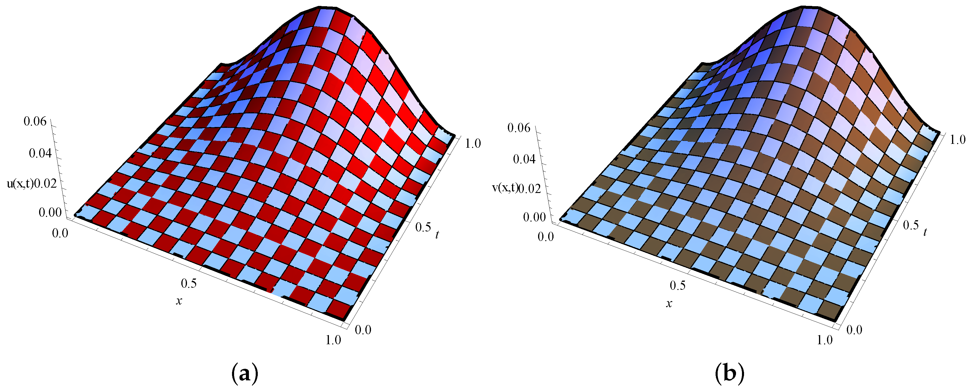
The exact solutions are U ( x , t ) = V ( x , t ) = x 2 ( x 1 ) 2 t 2 [48]. In Table 2, the computational results exhibit the value of U ( x , t ) and V ( x , t ) at different stages of x, for Example 1. In Table 3 and Table 4, the L of U ( x , t ) are estimated on λ = 0.1 , 0.3 and 0.5 for different values of N and provide an analysis of the convergence order between stages. In Table 5, L and an order of convergence assessment are conducted for U ( x , t ) at different values of τ when λ = 0.1 , 0.005 .
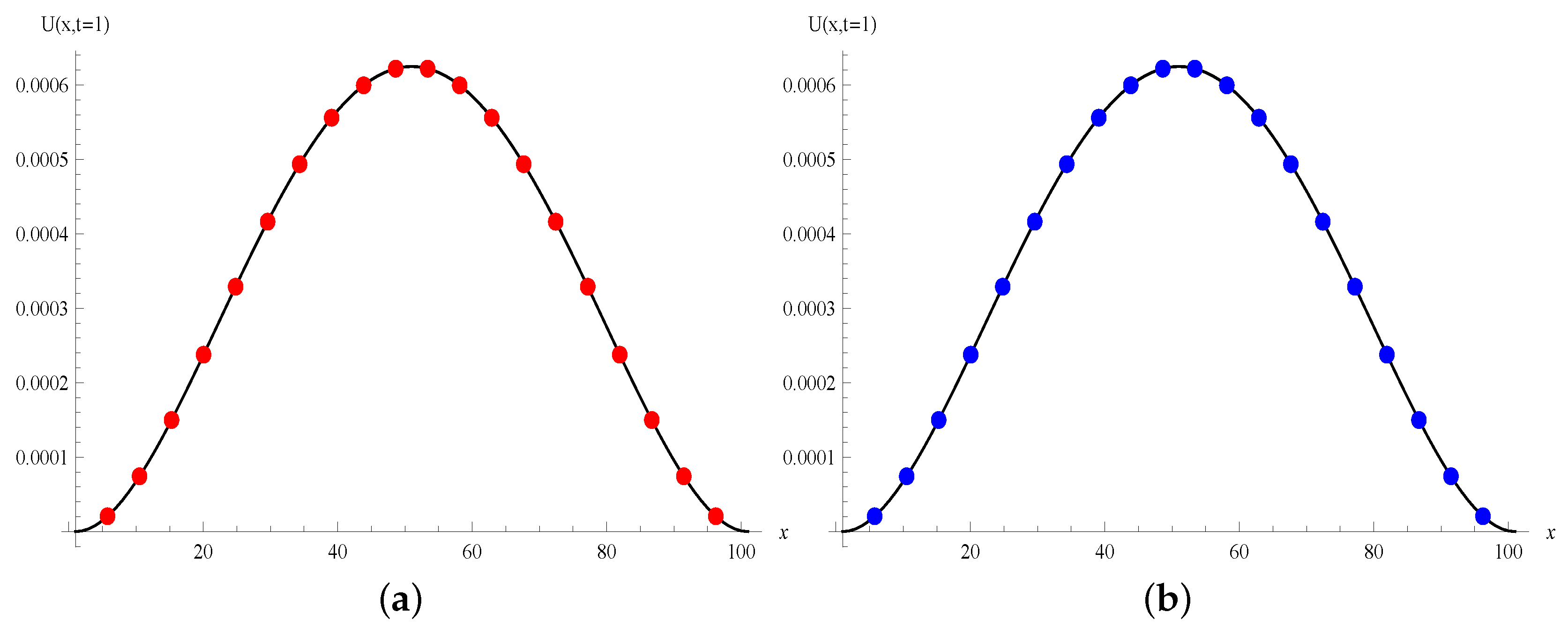
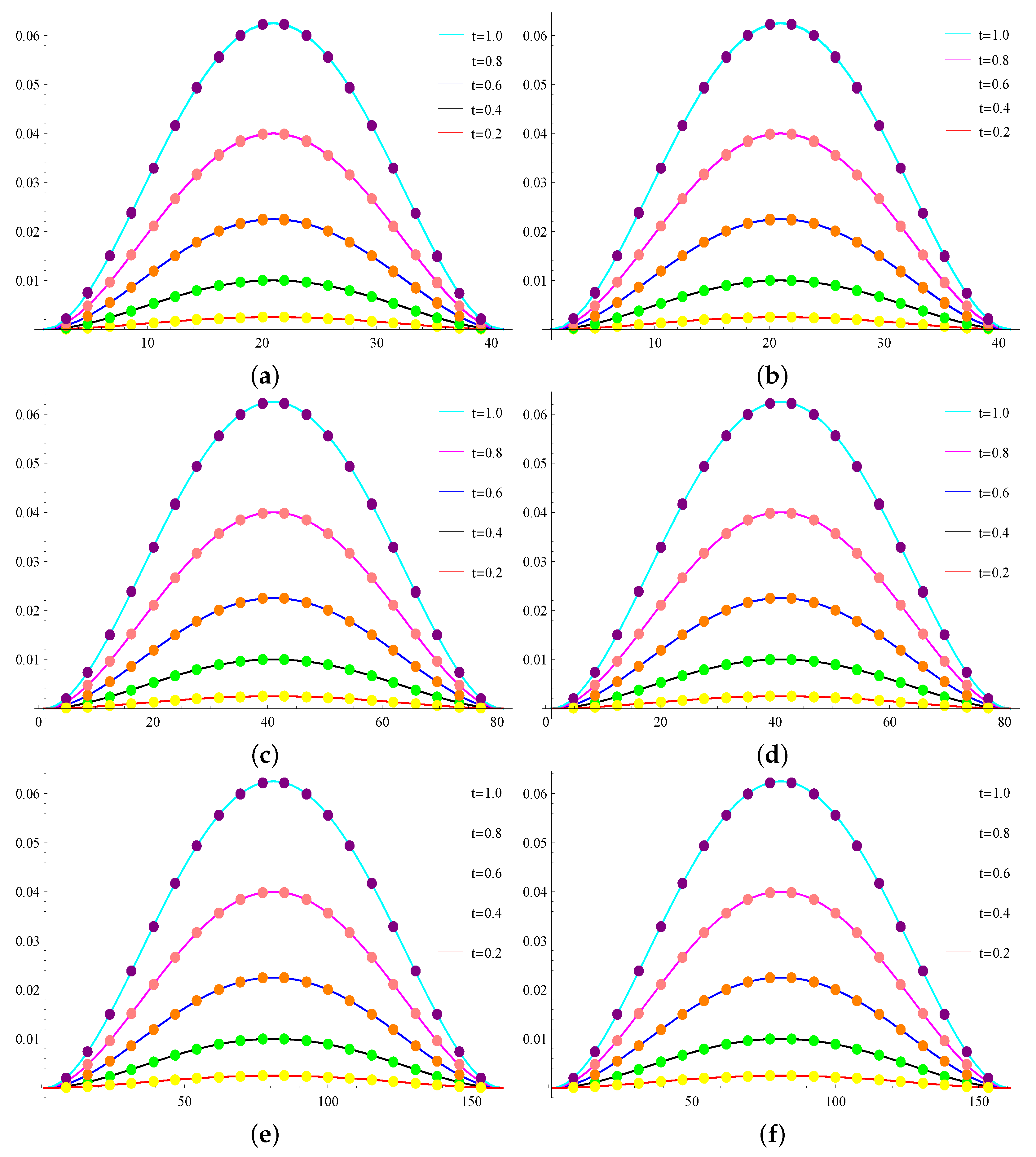
Figure 1 shows the exact 3D solution, while Figure 2 represents the comparison of 2D exact and approximate values U and V using N = 100 , Δ t = 0.001 , and λ = 0.1 . The convergence of the exact and approximate solutions is illustrated in Figure 3 at different time stages for Example 1. In Figure 4, the graphs display the function error for different values of N and λ .
In Figure 4, graphs show the error function (EF) for different value of N and λ .
Example 2.
Consider the TFCBE in the Caputo sense, when γ = 1000 and α 1 = α 2 = 0.001 ,
λ U t λ 2 U x 2 + γ U U x + α 1 ( U V ) x = Q 1 λ V t λ 2 V x 2 + γ V V x + α 2 ( U V ) x = Q 2 a x b , 0 t T , 0 < λ < 1
where BCs and ICs are u ( 0 , t ) = v ( o , t ) = t 2 u ( 1 , t ) = v ( 1 , t ) = t 2 e and u ( x , 0 ) = 0 v ( x , 0 ) = 0 , respectively.
The exact solutions are U ( x , t ) = V ( x , t ) = t 2 e x . For Example 2, Table 6 displays the computational results showing the values of the function at various stages, while Table 7 represents the behaviour of the error norm for different values of k at λ = 0.1 and 0.05 .
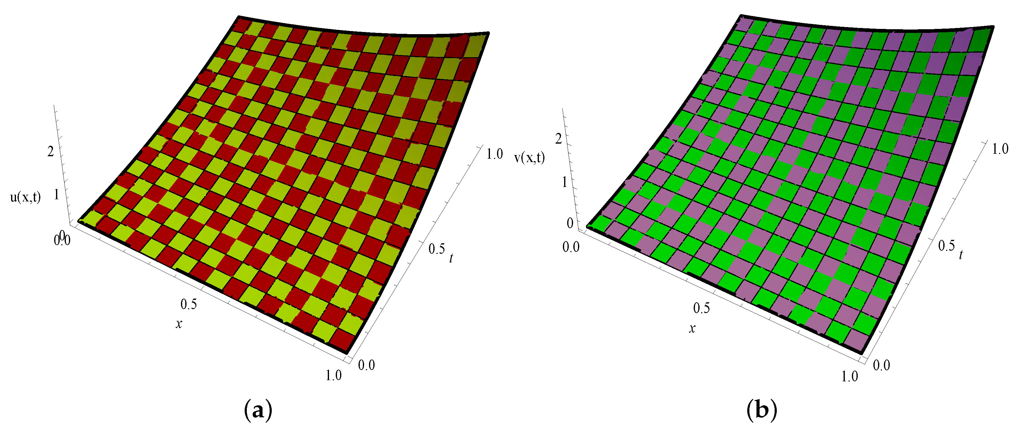
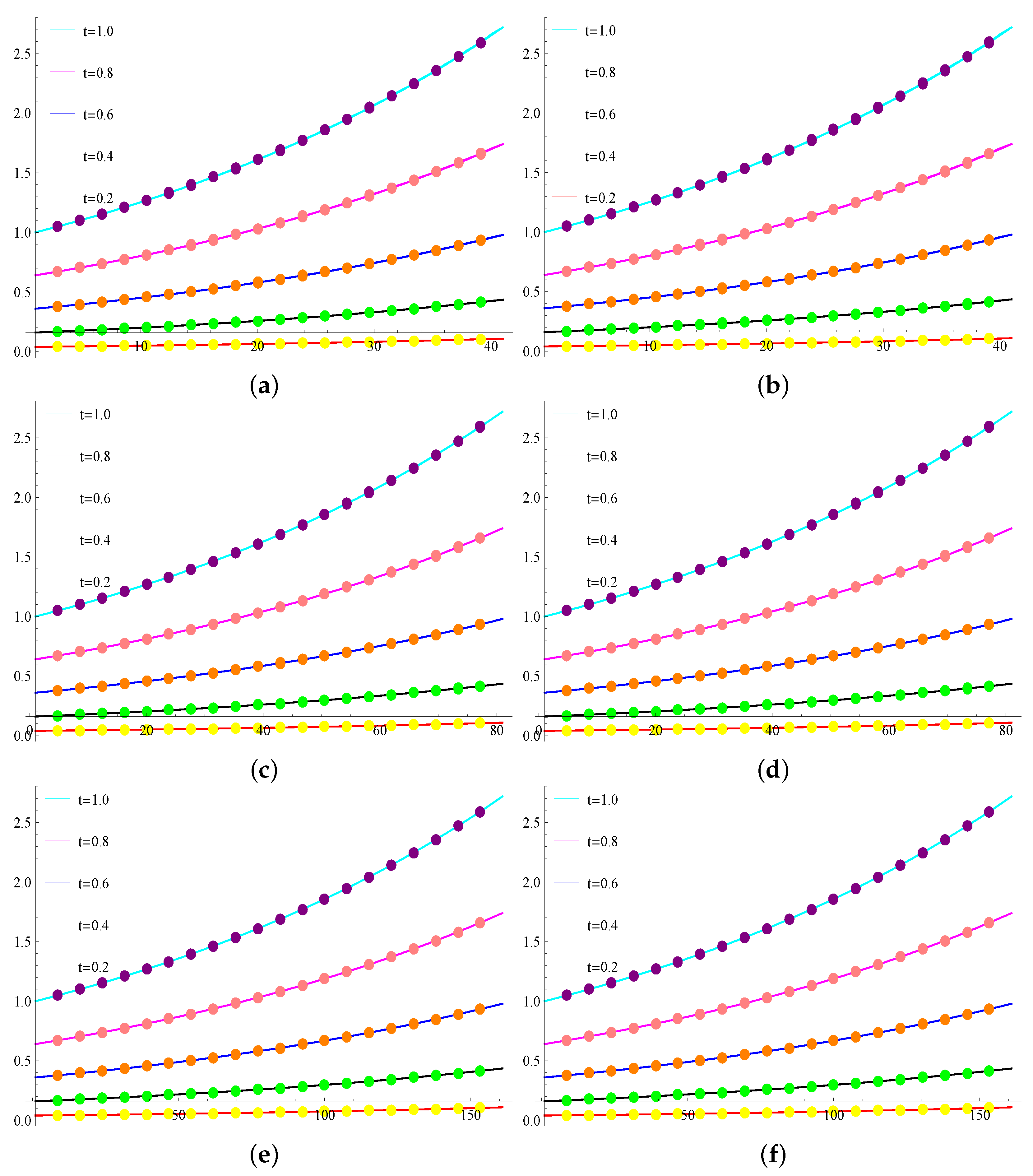
Figure 5 shows the exact 3D solution, while Figure 6 represents the comparison of the exact and approximate 2D solutions for U and V using N = 100 , Δ t = 0.001 , and λ = 0.1 . For Example 2, Figure 7 illustrates the convergence of the exact and approximate solution at different stages. In Figure 8, the graphs display the function error for different values of N and λ .

7. Conclusion Remarks

In the conducted research, we have developed the efficient approximate method for TFCBEs. It is used to study turbulent fluids, suspensions, and the propagation of shallow water waves. Here, we obtain a approximate solution for TFCBEs using the CBS and Crank–Nicolson method. The time FD has been discretized using Caputo’s formula. The numerical algorithm shows that the system is unconditionally stable. The numerical order of convergence has also been determined. Two numerical test problems have been considered in order to evaluate the effectiveness of the delivered method. The results presented in the tables and graphs demonstrate the applicability and accuracy of the presented technique. Approximated values have been compared with exact values, and their errors have been determined. The numerical results were calculated using Mathematica 12.3, and our method yielded acceptable outcomes.

Author Contributions

Conceptualization, U.G., M.A. and T.A.; Funding acquisition, E.K.E.-S., M.A.E.A. and N.F.A.; Investigation, U.G., M.A. and T.A.; Methodology, U.G., M.A. and T.A.; Project administration, E.K.E.-S., M.A.E.A. and N.F.A.; Resources, M.A.; Software, U.G., M.A., M.A.E.A. and N.F.A.; Supervision, M.A.; Validation, U.G., M.A., T.A., E.K.E.-S., M.A.E.A. and N.F.A.; Writing—original draft, U.G., M.A., T.A., E.K.E.-S., M.A.E.A. and N.F.A.; Writing—review & editing, U.G., E.K.E.-S., M.A.E.A. and N.F.A. All authors have read and agreed to the published version of the manuscript.

Funding

The Deputyship for Research & Innovation in the Ministry of Education in Saudi Arabia funded this research work through project number 445-9-492.

Data Availability Statement

Data are contained within the article.

Acknowledgments

The authors extend their appreciation to the Deputyship for Research & Innovation, Ministry of Education in Saudi Arabia for funding this research work (project number 445-9-492). The authors are also grateful to the anonymous referees for their valuable suggestions, which significantly improved this manuscript.

Conflicts of Interest

The authors declare no conflict of interest.

References

  1. Burgers, J.M. A mathematical model illustrating the theory of turbulence. Adv. Appl. Mechanics. 1948, 1, 171–199. [Google Scholar]
  2. Cole, J.D. On a quasi-linear parabolic equation occurring in aerodynamics. Q. Appl. Math. 1951, 9, 225–236. [Google Scholar] [CrossRef]
  3. Esipov, S.E. Coupled Burgers equations: A model of polydispersive sedimentation. Phys. Rev. E 1995, 52, 3711. [Google Scholar] [CrossRef] [PubMed]
  4. Nee, J.; Duan, J. Limit set of trajectories of the coupled viscous Burgers equations. Appl. Math. Lett. 1998, 11, 57–61. [Google Scholar] [CrossRef]
  5. Logan, J.D. An Introduction to Nonlinear Partial Differential Equations; John Wiley & Sons: Hoboken, NJ, USA, 2008; Volume 89. [Google Scholar]
  6. Caputo, M.; Fabrizio, M. A new definition of fractional derivative without singular kernel. Prog. Fract. Differ. Appl. 2015, 1, 113. [Google Scholar]
  7. Li, C.; Zeng, F. Numerical Methods for Fractional Calculus; CRC Press: New York, NY, USA, 2015. [Google Scholar]
  8. Gorenflo, R.; Mainardi, F. Fractional Calculus: Integral and Differential Equations of Fractional Order; Springer: Vienna, Austria, 1997; pp. 223–276. [Google Scholar]
  9. Chen, Y.; An, L.H. Numerical solutions of coupled Burgers equations with time and space-fractional derivatives. Appl. Math. Comput. 2008, 200, 87–95. [Google Scholar] [CrossRef]
  10. Khan, N.A.; Ara, H.; Mahmood, A. Numerical solutions of time-fractional Burgers equations. Int. J. Numer. Methods Heat Fluid Flow 2012, 22, 175–193. [Google Scholar]
  11. Prakash, A.; Kumar, M.; Sharma, K.K. Numerical method for solving fractional coupled Burgers equations. Int. J. Numer. Methods Heat Fluid Flow 2015, 260, 314–320. [Google Scholar] [CrossRef]
  12. Singh, J.; Kumar, D.; Swroop, R. Numerical solution of time- and space-fractional coupled Burgers’ equations via homotopy algorithm. Alex. Eng. J. 2016, 55, 1753–1763. [Google Scholar] [CrossRef]
  13. Aminikhah, H.; Malekzadeh, N. An efficient method for systems of variable coefficient Coupled Burgers’ equation with time-fractional derivative. Sci. World J. 2013, 2013, 687695. [Google Scholar] [CrossRef]
  14. Ahmed, H.F.; Baghat, M.S.M.; Zaki, M. Analytical approaches to space and time fractional coupled Burgers’ equations. Pramana 2019, 92, 38. [Google Scholar] [CrossRef]
  15. Albouhimad, B.; Adibi, H. On a hybrid spectral exponential Chebyshev method for time-fractional coupled Burgers equations on a semi-infinite domain. Adv. Differ. Equ. 2017, 2017, 85. [Google Scholar] [CrossRef]
  16. Sulaiman, T.A.; Yavuz, M.; Bulut, H.; Baskonus, H.M. Investigation of the fractional coupled viscous Burgers; equation involving Mittag-Leffler kernel. Stat. Mech. Its Appl. 2019, 527, 121–126. [Google Scholar] [CrossRef]
  17. Liu, J.; Hou, G. Numerical solutions of the space and time fractional coupled Burgers equations by generalized differential transform method. Appl. Math. Comput. 2011, 217, 7001–7008. [Google Scholar] [CrossRef]
  18. Ozdemir, N.; Secer, A.; Bayram, M. The gegenbauer wavelets-based computational methods for the coupled system of Burgers equations with time fractional derivative. Mathematics 2019, 7, 486. [Google Scholar] [CrossRef]
  19. Abazari, R.; Borhanifar, A. Numerical study of the solution of the burgers and coupled burgers equations by a differential transformation method. Comput. Appl. 2010, 59, 2711–2722. [Google Scholar] [CrossRef]
  20. Mittal, R.; Arora, G. Numerical solution of the coupled viscous burgers equation. Commun. Nonlinear Sci. Numer. Simul. 2011, 16, 1304–1313. [Google Scholar] [CrossRef]
  21. Shukla, H.; Tamsir, M.; Srivastava, V.K.; Kumar, J. Numerical solution of two dimensional coupled viscous burger equation using modified cubic b-spline differential quadrature method. AIP Adv. 2014, 4, 117134. [Google Scholar] [CrossRef]
  22. Kumar, A.; Arora, R. Solutions of the coupled system of burgers equations and coupled klein-gordon equation by rdt method. Int. J. Adv. Appl. Math. Mech. 2013, 1, 103–115. [Google Scholar]
  23. Srivastava, V.K.; Tamsir, M.; Awasthi, M.K.; Singh, S. One dimensional coupled burgers equation and its numerical solution by an implicit logarithmic finite difference method. AIP Adv. 2014, 4, 037119. [Google Scholar] [CrossRef]
  24. Mittal, R.; Tripathi, A. A collocation method for numerical solutions of coupled burgers equations. Int. J. Comput. Methods Eng. Sci. Mech. 2014, 15, 457–471. [Google Scholar] [CrossRef]
  25. Sarboland, M.; Aminataei, A. An efficient numerical scheme for coupled nonlinear burgers equations. Appl. Math. Inf. Sci. 2015, 9, 245–255. [Google Scholar] [CrossRef]
  26. Salih, H.M.; Tawfiq, L.N.M.; Yahya, Z.R. Numerical solution of the coupled viscous burgers equation via cubic trigonometric b-spline approach. Math Stat. 2016, 2, MSOA-2-011. [Google Scholar]
  27. He, Y.; Tang, X. Numerical simulations of a family of the coupled viscous burgers equation using the lattice Boltzmann method3. J. Stat. Mech. Theory Exp. 2016, 2016, 023208. [Google Scholar] [CrossRef]
  28. Chuathong, N.; Kaennakham, S. Numerical solution to coupled burgers equations by gaussian based hermite collocation scheme. J. Appl. Math. 2018, 2018, 3416860. [Google Scholar] [CrossRef]
  29. Jima, M.; Shiferaw, A.; Tsegaye, A. Numerical solution of the coupled viscous burgers equation using differential quadrature method based on fourier expansion basis. Appl. Math. 2018, 9, 821. [Google Scholar] [CrossRef]
  30. Oruc, O.; Bulut, F.; Esen, A. Chebyshev wavelet method for numerical solutions of coupled burgers equation. Hacet. J. Math. Stat. 2019, 48, 1–16. [Google Scholar]
  31. Wu, G.C.; Zeng, D.Q.; Baleanu, D. Fractional impulsive differential equations: Exact solutions, integral equations and short memory case. Fract. Calc. Appl. Anal. 2019, 22, 180–192. [Google Scholar] [CrossRef]
  32. Dubey, V.P.; Singh, J.; Alshehri, A.M.; Dubey, S.; Kumar, D. Analysis of local fractional coupled Helmholtz and coupled Burgers’ equations in fractal media. AIMS Math. 2022, 7, 8080–8111. [Google Scholar] [CrossRef]
  33. Wang, K.J. New exact solutions of the local fractional modified equal width-Burgers equation on the Cantor sets. FRACTALS (Fractals) 2023, 31, 1–9. [Google Scholar] [CrossRef]
  34. Nazir, T.; Abbas, M.; Iqbal, M.K. New cubic B-spline approximation technique for numerical solutions of coupled viscous Burgers equations. Eng. Comput. 2021, 38, 83–106. [Google Scholar] [CrossRef]
  35. De Boor, C.; De Boor, C. A Practical Guide to Splines; Springer: New York, NY, USA, 1978; Volume 27, p. 325. [Google Scholar]
  36. Koch, P.E.; Lyche, T.; Neamtu, M.; Schumaker, L.L. Control curves and knot insertion for trigonometric splines. Adv. Comput. Math. 1995, 3, 405–424. [Google Scholar] [CrossRef]
  37. Lin, Y.; Xu, C. Finite difference/spectral approximations for the timefractional diffusion equation. J. Comput. Phys. 2007, 2225, 1533–1552. [Google Scholar] [CrossRef]
  38. Sayevand, K.; Yazdani, A.; Arjang, F. Cubic B-spline collocation method and its application for anomalous fractional diffusion equations in transport dynamic systems. J. Vib. Control 2016, 22, 2173–2186. [Google Scholar] [CrossRef]
  39. Ru, J.G.Y. B-Spline for Initial and Boundary Value Problems. Ph.D. Thesis, Universiti Sains Malaysia, Penang, Malaysia, 2012. [Google Scholar]
  40. Abbas, M.; Majid, A.A.; Md. Ismail, A.I.; Rashid, A. Numerical method using cubic B-spline for a strongly coupled reaction-diffusion system. PLoS ONE 2014, 9, e83265. [Google Scholar] [CrossRef]
  41. Rubin, S.G.; Graves, R.A.; Arjang, F. A Cubic Spline Approximation for Problems in Fluid Mechanics; NASA TR R-436; NASA: Washington, DC, USA, 1975.
  42. Smith, G.D. Numerical Solution of Partial Differential Equations: Finite Difference Methods; Oxford University Press: Oxford, UK, 1985. [Google Scholar]
  43. Akram, T.; Abbas, M.; Ali, A.; Iqbal, A.; Baleanu, D. A numerical approach of a time fractional reaction–diffusion model with a non-singular kernel. Symmetry 2020, 12, 1653. [Google Scholar] [CrossRef]
  44. Akram, T.; Abbas, M.; Ali, A. A numerical study on time fractional fisher equation using an extended cubic b-spline approximation. J. Math. Comput. Sci. 2021, 22, 85–96. [Google Scholar] [CrossRef]
  45. Iqbal, M.k.; Abbas, M.; Nazir, T.; Ali, N. Application of new quintic polynomial b-spline approximation for numerical investigation of kuramoto-sivashinsky equation. Adv. Differ. Equ. 2020, 2020, 558. [Google Scholar] [CrossRef]
  46. Siddiqi, S.S.; Arshed, S. Quintic B-spline for the numerical solution of the good Boussinesq equation. J. Egypt. Math. Soc. 2014, 22, 209–213. [Google Scholar]
  47. Poulin, J.R. Calculating Infinite Series Using Parseval’s Identity; The University of Maine: Orono, ME, USA, 2020. [Google Scholar]
  48. Taghipour, M.; Aminikhah, H. A B-Spline Quasi Interpolation Crank–Nicolson Scheme for Solving the Coupled Burgers Equations with the Caputo–Fabrizio Derivative. Math. Probl. Eng. 2021, 2021, 8837846. [Google Scholar] [CrossRef]
Figure 1. Exact 3D solutions for Example 1. (a) For U; (b) For V.
Fractalfract 08 00093 g001
Figure 2. For Example 1, Comparison between 2D Exact and Approximate solution. (a) For U, (b) For V.
Fractalfract 08 00093 g002
Figure 3. For Example 1, Exact and Approximate solutions at different time stages. (a) N = 40 , Δ t = 1 / 32 and λ = 0.1 of U, (b) N = 40 , Δ t = 1 / 32 and λ = 0.1 of V, (c) N = 80 , Δ t = 1 / 64 and λ = 0.5 of U, (d) N = 80 , Δ t = 1 / 64 and λ = 0.5 of V, (e) N = 160 , Δ t = 1 / 132 and λ = 0.9 of U, (f) N = 160 , Δ t = 1 / 132 and λ = 0.9 of V.
Fractalfract 08 00093 g003
Figure 4. Error graph at different stages for Example 1. (a) EF for U, when λ = 0.1 and Δ t = 1 / 1000 . (b) EF for V, when λ = 0.1 and Δ t = 1 / 1000 . (c) EF for U, when N = 100 and Δ t = 1 / 100 . (d) EF for V, when N = 100 and Δ t = 1 / 100 .
Fractalfract 08 00093 g004
Figure 5. Exact 3D solutions for Example 2. (a) For U; (b) For V.
Fractalfract 08 00093 g005
Figure 6. For Example 2 Comparison between Exact and Approximate 2D solution. (a) For U; (b) For V.
Fractalfract 08 00093 g006
Figure 7. For Example 2, exact and approximate solutions at different time stages. (a) N = 40 , Δ t = 1 / 32 , and λ = 0.1 of U. (b) N = 40 , Δ t = 1 / 32 , and λ = 0.1 of V. (c) N = 80 , Δ t = 1 / 64 , and λ = 0.9 of U. (d) N = 80 , Δ t = 1 / 64 , and λ = 0.9 of V. (e) N = 160 , Δ t = 1 / 132 , and λ = 0.5 of U. (f) N = 160 , Δ t = 1 / 132 , and λ = 0.5 of V.
Fractalfract 08 00093 g007
Figure 8. Error graph of function at different stages for Example 2. (a) EF for U, when Δ t = 1 / 512 and λ = 0.1 . (b) EF for V, when Δ t = 1 / 512 and λ = 0.1 . (c) EF for U, when N = 100 and Δ t = 1 / 100 . (d) EF for V, when N = 100 and Δ t = 1 / 100 .
Fractalfract 08 00093 g008
Table 1. B i ( x ) , B i ( x ) , and B i ( x ) at the knots.
x i + 1 x i x i 1 Else
B i ( x ) 1 / 6 2 / 3 1 / 6 0
B i ( x ) 1 / 2 h 0 1 / 2 h 0
B i ( x ) 1 / h 2 2 / h 2 1 / h 2 0
Table 2. Absolute error of U ( x , t ) and V ( x , t ) at λ = 0.3 for Example 1, when Δ t = 1 1000 , and N = 100.
For U ( x , t ) For V ( x , t )
x ExactApproximatedErrorApproximatedError
SolutionSolutionSolution
0.1 0.00810.00809927.95989 × 10   7 0.00809927.95986 × 10   7
0.2 0.02560.02559918.90499 × 10   7 0.02559918.90497 × 10   7
0.3 0.04410.04409919.17458 × 10   7 0.04409919.17457 × 10   7
0.4 0.05760.05759901.01942 × 10   6 0.05759901.01942 × 10   6
0.5 0.06250.06249871.27097 × 10   6 0.06249871.27097 × 10   6
0.6 0.05760.05759821.82313 × 10   6 0.05759821.82313 × 10   6
0.7 0.04410.04409673.31485 × 10   6 0.04409673.31485 × 10   6
0.8 0.02560.02559109.02991 × 10   6 0.02559109.02991 × 10   6
0.9 0.00810.00808621.38116 × 10   5 0.00808621.38116 × 10   5
Table 3. Absolute error and order of convergence of U ( x , t ) when λ = 0.1 , 0.3 , 0.5 and Δ t = 0.001 for Example 1.
h L Order L Order L Order
λ = 0 . 1 λ = 0 . 3 λ = 0 . 5
1 / 20 3.39429 × 10   4 3.39353 × 10   4 3.39557 × 10   4
1 / 40 8.88467 × 10   5 1.933728.88382 × 10   5 1.933538.88819 × 10   5 1.93369
1 / 80 2.22587 × 10   5 1.996952.22520 × 10   5 1.997252.22364 × 10   5 1.99897
1 / 160 5.59571 × 10   6 1.991985.58911 × 10   6 1.993245.55831 × 10   6 2.00021
1 / 320 1.41227 × 10   6 1.986321.40599 × 10   6 1.984611.37167 × 10   6 2.01871
Table 4. Absolute error and order of convergence of U ( x , t ) when λ = 0.7 , 0.8 , 0.9 and Δ t = 0.001 for Example 1.
h L Order L Order L Order
λ = 0 . 7 λ = 0 . 8 λ = 0 . 9
1 / 20 3.39995 × 10   4 3.40177 × 10   4 3.40102 × 10   4
1 / 40 8.88670 × 10   5 1.935798.86860 × 10   5 1.939518.81345 × 10   5 1.94819
1 / 80 2.20861 × 10   5 2.008512.18047 × 10   5 2.024072.11294 × 10   5 2.06046
1 / 160 5.37405 × 10   6 2.039065.06770 × 10   6 2.105244.36195 × 10   6 2.27621
1 / 320 1.17911 × 10   6 2.188318.66987 × 10   7 2.547251.63195 × 10   6 1.88726
Table 5. Absolute error and order of convergence of U ( x , t ) when λ = 0.1 , 0.05 and N = 512 for Example 1.
τ L Order L Order
λ = 0 . 1 λ = 0 . 05
1 / 16 4.41715 × 10   4 4.41624 × 10   4
1 / 32 1.14146 × 10   4 1.952241.14119 × 10   4 1.95228
1 / 64 2.89674 × 10   5 1.978382.89596 × 10   5 1.97843
1 / 128 7.26223 × 10   6 1.995957.26003 × 10   6 1.99599
Table 6. Absolute error of U ( x , t ) and V ( x , t ) , when λ = 0.1 , Δ t = 0.001 , and N = 100 , for Example 2.
For U ( x , t ) For V ( x , t )
x ExactApproximatedErrorApproximatedError
SolutionSolutionSolution
0.1 1.105171.105172.99571 × 10   7 1.105172.99571 × 10   7
0.2 1.221401.221406.01967 × 10   7 1.221406.01967 × 10   7
0.3 1.349861.349869.10470 × 10   7 1.349869.10470 × 10   7
0.4 1.491821.491831.22815 × 10   6 1.491831.22815 × 10   6
0.5 1.648721.648721.55804 × 10   6 1.648721.55804 × 10   6
0.6 1.822121.822121.90185 × 10   6 1.822121.90185 × 10   6
0.7 2.013752.013752.25080 × 10   6 2.013752.25080 × 10   6
0.8 2.225542.225542.53167 × 10   6 2.225542.53167 × 10   6
0.9 2.718282.718282.35147 × 10   6 2.718282.35147 × 10   5
Table 7. Absolute error and order of convergence of U ( x , t ) when λ = 0.1 , 0.05 and N = 512 for Example 2.
τ L Order L Order
λ = 0 . 1 λ = 0 . 05
1 / 64 1.63599 × 10   3 1.63597 × 10   3
1 / 128 4.10724 × 10   4 1.993924.10713 × 10   4 2.01259
1 / 256 1.01791 × 10   4 2.012561.01786 × 10   4 2.01259
1 / 512 2.42205 × 10   5 2.071312.42145 × 10   5 2.07159
Disclaimer/Publisher’s Note: The statements, opinions and data contained in all publications are solely those of the individual author(s) and contributor(s) and not of MDPI and/or the editor(s). MDPI and/or the editor(s) disclaim responsibility for any injury to people or property resulting from any ideas, methods, instructions or products referred to in the content.