Article

The Application of Fractional Derivative Viscoelastic Models in the Finite Element Method: Taking Several Common Models as Examples

1
National Engineering Laboratory of Highway Maintenance Technology, Changsha University of Science & Technology, Changsha 410114, China
2
Xinjiang Key Laboratory of Green Construction and Smart Traffic Control of Transportation Infrastructure, Xinjiang University, Urumqi 830017, China
3
Key Laboratory of Special Environment Road Engineering of Hunan Province, Changsha University of Science & Technology, Changsha 410114, China
*
Author to whom correspondence should be addressed.
Fractal Fract. 2024, 8(2), 103; https://doi.org/10.3390/fractalfract8020103
Submission received: 11 January 2024 / Revised: 1 February 2024 / Accepted: 2 February 2024 / Published: 7 February 2024
(This article belongs to the Section Engineering)

Abstract

:
This paper aims to incorporate the fractional derivative viscoelastic model into a finite element analysis. Firstly, based on the constitutive equation of the fractional derivative three-parameter solid model (FTS), the constitutive equation is discretized by using the Grünwald–Letnikov definition of the fractional derivative, and the stress increment and strain increment relationship and Jacobian matrix are obtained by using the difference method. Subsequently, we degrade the model to establish stress increment and strain increment relationships and Jacobian matrices for the fractional derivative Kelvin model (FK) and fractional derivative Maxwell model (FM). Finally, we further degrade the fractional derivative viscoelastic model to derive stress increment and strain increment relationships and Jacobian matrices for a three-component solid model and Kelvin and Maxwell models. Based on these developments, a UMAT subroutine is implemented in ABAQUS 6.14 finite element software. Three different loading modes, including static load, dynamic load, and mobile load, are analyzed and calculated. The calculations primarily involve a convergence analysis, verification of numerical solutions, and comparative analysis of responses among different viscoelastic models.

1. Introduction

The fractional derivative viscoelastic model has been extensively studied and proven to require only a few parameters for the constitutive modeling of viscoelastic materials, enabling an accurate description of material mechanical properties across a wide frequency range. Compared with traditional viscoelastic models, this approach offers enhanced precision in characterizing the viscoelastic behavior of materials. Ronald L. Bagley et al. [1] have highlighted the suitability of fractional derivatives in describing the dynamic frequency response process of viscoelastic materials. The solution to fractional calculus is more intricate than integral calculus, primarily influenced by two factors. Firstly, unlike integral calculus, fractional calculus necessitates storing historical data throughout the entire calculation period. As time progresses, the accumulation of historical information leads to an increase in computational workload. Secondly, as time passes, controlling discrete errors becomes progressively challenging and results in a growing deviation between calculated results and accurate values [2]. Due to the continuous advancement and refinement of viscoelastic constitutive theory, numerical calculation methods, and computer hardware, the finite element method has been widely applied in the mechanical analysis of viscoelastic structures [3,4]. It is necessary to store the stress–strain history at each Gaussian point to implement a fractional derivative viscoelastic model [5]. One approach is to utilize a Common Block (CB) in Fortran programming, which allows for information exchange between program units by storing each strain–stress component at every increment. However, after conducting trial calculations, it was discovered that the CB storage capacity is limited to 2 GB. Alternatively, historical stress–strain data can be stored in a TXT file; however, this method results in slower program execution speed. Compared with these two methods, there is a preference for storing historical stress–strain data in CB due to its advantages. The storage size mainly depends on the number of incremental steps and the number of Gaussian points (which correlates with grid quantity).
Numerous scholars have extensively researched the numerical computation of fractional derivative viscoelastic models. J. Padovan [6] investigated various finite element implementation methods for differential operators, deriving implicit, explicit, and predictive correction transient algorithms for viscoelastic finite element simulation based on numerical labels assigned to fractional order operators. R.C. Koeller [7] investigated fractional derivative viscoelastic models for genetic integrals and derived creep and relaxation functions for various fractional calculus models. Mikael Enelund et al. [8] employed the fractional derivative viscoelastic model of genetic integration in a finite element analysis. They expanded the constitutive model to encompass the three-dimensional stress states of isotropic materials. Gioacchino Alotta et al. [5,9] introduced the numerical computation of a series of isotropic three-dimensional fractional derivative viscoelastic constitutive models using user-defined material subroutines in ABAQUS software. Li Zhuo et al. [10] presented the finite element formulation for the viscoelastic fractional derivative and employed a modal analysis to decouple the equation of motion. The time-domain and frequency-domain responses of the decoupled single-degree-of-freedom system were computed using the Laplace transform and its inverse counterpart. Using the fractional derivative Kelvin model, Liu Linchao et al. [11] formulated the fractional derivative dynamic finite element equation of a viscoelastic damper subjected to external forces. They obtained the numerical solution through Newmark’s numerical integration method. It has been demonstrated that Zhang and Shimizu’s fractional derivative numerical integration method satisfies the requirements of accuracy, convergence, and stability. Yin Hua et al. [12] incorporated the fractional derivative three-element model into the finite element model. Using this constitutive relationship, they derived the finite element scheme for analyzing viscoelastic structural dynamics. Additionally, a numerical algorithm based on fractional derivative equations was employed to obtain the numerical solution of the finite element scheme, with a focus on investigating the dynamic viscoelastic response of two-dimensional asphalt pavement structures. Hiroshi Nasuno et al. [13] proposed a fractional derivative finite deformation theory and nonlinear finite element method to assess the dynamic characteristics of viscoelastic bodies employed for vibration reduction. They developed a nonlinear finite element calculation program for evaluating the vibration characteristics of viscoelastic products. Masataka Fukunaga et al. developed a fractional derivative constitutive model [14], and commercial finite element (FE) software was employed to solve the dynamic problem associated with gel-like materials. Ana Cristina Galucio et al. [15] proposed a finite element formula for a transient dynamic analysis of sandwich beams containing embedded viscoelastic materials based on fractional derivative constitutive equations. The sandwich configuration consists of a viscoelastic core (based on Timoshenko theory) sandwiched between an elastic surface (based on the Euler–Bernoulli hypothesis). The viscoelastic model used to describe core behavior is a four-parameter fractional derivative. Silvio Sorrentino et al. [16] proposed a method to reduce computational complexity when employing the fractional derivative Kelvin Voigt model for a finite element analysis of vibrating linear systems, which can be extended to other linear models involving fractional derivatives. The computation is optimized by transforming the high-dimensional principal feature problem into two lower-dimensional standard-related feature problems. Fernando Cortés et al. [17] proposed a finite element formulation designed explicitly for a transient dynamic analysis of free-layer damping plates, wherein the viscoelastic behavior of the damping layer is modeled using a fractional derivative. The efficacy of this approach was experimentally validated. Giuseppe Catania et al. [18] proposed a compression technique based on the computation of two reduced-size feature problems, utilizing either the fractional Zener model or the fractional standard linear entity model as rheological models, which are also applicable for designing linear models with varying fractional orders. Marcin Kamiński et al. [19] employed the stochastic finite element method (SFEM) to investigate the natural vibration characteristics of a thin Kirchhoff Love plate supported by a time-fractional viscoelastic medium, where the mechanical behavior of the support was described using the Riemann–Liouville fractional derivative. Alba Sofi [20] investigated the time-domain response calculation of nonlinear beams incorporating fractional derivative elements subjected to moving loads. It proposed an innovative fractional integration technique, the Improved Pseudo-force method (IPFM), for solving a specific class of nonlinear fractional differential equations with time-varying generalized coordinates. Giovanni Malara et al. [21] investigated the problem of efficiently computing the nonlinear response of a rod with a fractional derivative constitutive model under random excitation. They proposed an approximate analytical solution based on statistical linearization technology and developed a boundary element-based method (BEM) to estimate the response statistics of the rod numerically. Boonme Chinnaboon et al. [22] proposed an analytical model based on the fractional derivative Kelvin Voigt model of orthotropic plates. They investigated the influence of viscoelastic foundation parameters and the ratio of the elastic modulus on the bending response of the foundation. Xu-bing Xu et al. [23] proposed the fractional derivative Merchant (FDM) model for Shanghai Marine soil, developed a finite element program in ABAQUS to implement the FDM model, and utilized the program to conduct creep test simulations. By analyzing the triaxial creep and shear test results of deep artificial frozen soil, Dongwei Li et al. [24] established a fractional derivative constitutive model for deep frozen soil based on the Nishihara model. They developed the corresponding constitutive finite element model. The user subroutine of ADINA commercial finite element software was employed to simulate the artificial freezing curtain in a deep coal mine, and the numerical simulation results exhibited excellent agreement with field-measured data. The dynamic modulus and semi-circular bending test of an asphalt mixture were numerically simulated using the fractional Zener model (FZM) and the improved fractional Zener model (MFZM) in ABAQUS software by Qipeng Zhang et al. [25]. The experimental results exhibited excellent agreement with the simulation results obtained from MFZM. Yin Hua et al. [26] developed a two-dimensional finite element model of asphalt pavement structure based on the fractional derivative viscoelastic model of an asphalt mixture. They conducted a numerical analysis of the interaction between the vehicle and asphalt pavement coupling system.
In this paper, we derive the stress–strain relationship of the fractional derivative Kelvin model, fractional derivative Maxwell model, and fractional derivative three-element model (i.e., four-parameter model). Additionally, we obtain the relationship between stress and strain and the Jacobian matrix under a three-dimensional stress state. Subsequently, we develop a UMAT subroutine using the finite element software ABAQUS. As a typical viscoelastic material, the rubber-modified asphalt mixture has prominent time–temperature characteristics in its dynamic modulus. Existing classical viscoelastic models cannot sufficiently characterize the time–temperature characteristics of the material. Research has found that the fractional derivative model can better describe the time–temperature characteristics of the material with fewer parameters, making it easy to analyze and calculate. This article takes a rubber-modified asphalt mixture as an example and conducts finite element calculations. Firstly, a convergence analysis is conducted for static, dynamic, and moving loads based on the fractional derivative three-element model. Next, we apply this model to degenerate into an integer solution three-element model and verify its numerical solution. Finally, different types of classical and fractional derivative viscoelastic models are employed to analyze and calculate three separate finite element models: static, dynamic, and moving.

2. Finite Element Method

2.1. Fractional Derivative Viscoelastic Model

Existing literature shows that when calculating fractional derivatives, all scholars decompose and calculate fractional stress, strain, and other variables using the Grunwald–Letnikov definition:
D α x t = lim h 0 h α j = 1 N + 1 λ j x t + h j h
of which λ 1 = 1 , λ j + 1 = j 1 α λ j / j , h = t / N .
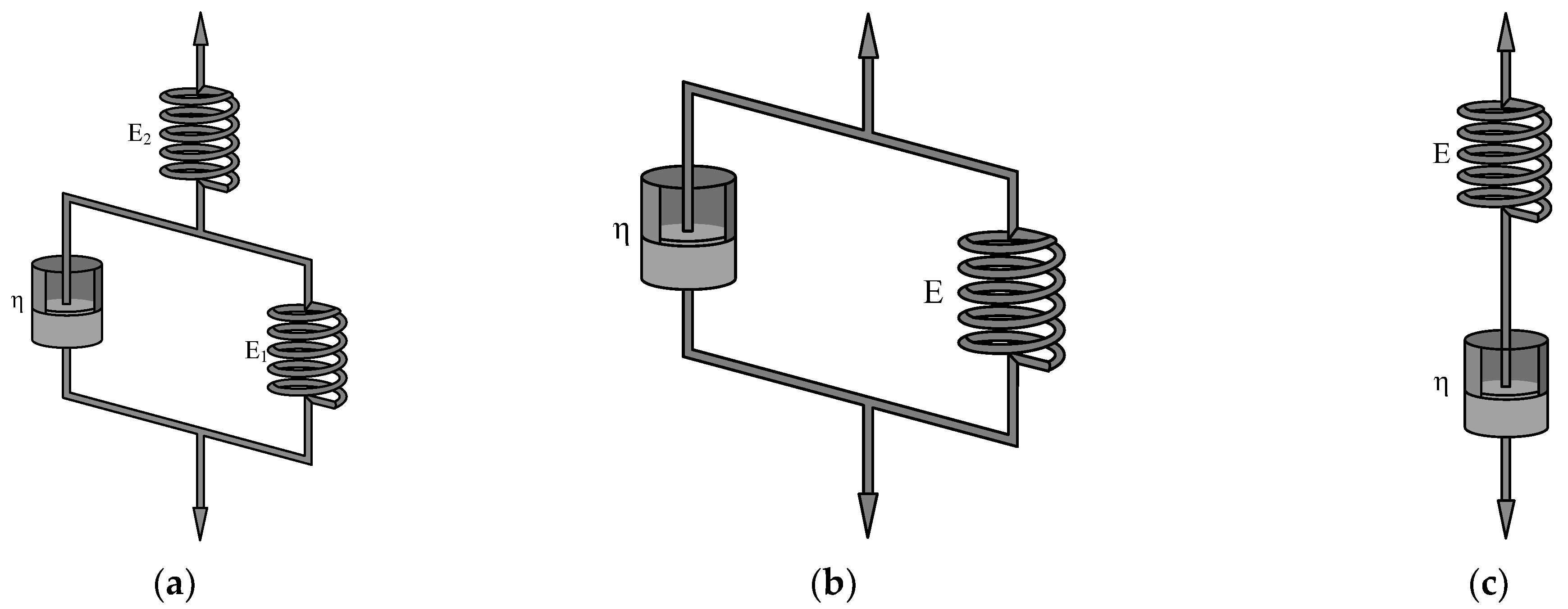
The FTS model, the FK model, and the FM model are depicted in Figure 1. These models comprise springs and Abel’s clay pots.
To realize the correspondence between the finite element solution and the theoretical solution, the finite element constitutive equation is defined from the Jacobian matrix of the theoretical solution. For the isotropic FTS, the constitutive relationship is as follows:
1 + η / E 1 + E 2 d α σ i i = E 2 E 1 + η d α ε i i / E 1 + E 2 / 1 + μ + 3 μ E 2 E 1 + η d α ε h / E 1 + E 2 / 1 + μ / 1 2 μ 1 + η / E 1 + E 2 d α σ i j = E 2 E 1 + η d α ε i j / E 1 + E 2 / 1 + μ
of which ε h = ε 11 + ε 22 + ε 33 / 3 , i , j = 1 , 2 , 3 i j , E1 and E2 are spring parameters, and η and α are Abel’s parameters.
Starting from the Grünwald–Letnikov definition of the fractional derivative, the above formula is expanded as follows:
σ i i N h = A ε i i N h + B ε h N h + C m = 2 N + 1 λ m ε i i N h + h m h + D m = 2 N + 1 λ m ε h N h + h m h E m = 2 N + 1 λ m σ i i N h + h m h σ i j N h = A ε i j N h + C m = 2 N + 1 λ m ε i j N h + h m h E m = 2 N + 1 λ m σ i j N h + h m h
of which A = E 2 E 1 h α + η / 1 + μ / E 1 + E 2 h α + η B = 3 μ E 2 E 1 h α + η / 1 2 μ / 1 + μ / E 1 + E 2 h α + η C = E 2 η / 1 + μ / E 1 + E 2 h α + η D = 3 μ E 2 η / 1 2 μ / 1 + μ / E 1 + E 2 h α + η E = η / E 1 + E 2 h α + η .
When calculating statics or implicit dynamics, the shear strain is the engineering shear strain, which can be written as
σ i i N h = A ε i i N h + B ε h N h + C m = 2 N + 1 λ m ε i i N h + h m h + D m = 2 N + 1 λ m ε h N h + h m h E m = 2 N + 1 λ m σ i i N h + h m h σ i j N h = A γ i j N h / 2 + C m = 2 N + 1 λ m γ i j N h + h m h / 2 E m = 2 N + 1 λ m σ i j N h + h m h
According to Equation (4), the relationship between the stress increment and strain increment can be obtained as follows:
Δ σ i i = A Δ ε i i + B Δ ε h + C m = 2 N + 1 λ m ε i i N + 1 h + h m h ε i i N h + h m h + D m = 2 N + 1 λ m ε h N + 1 h + h m h ε h N h + h m h E m = 2 N + 1 λ m σ i i N + 1 h + h m h σ i i N h + h m h Δ σ i j = A Δ γ i j / 2 + C m = 2 N + 1 λ m γ i j N + 1 h + h m h γ i j N h + h m h / 2 E m = 2 N + 1 λ m σ i j N + 1 h + h m h σ i j N h + h m h
According to formula (5), its Jacobian matrix can be obtained as follows:
c 11 = c 22 = c 33 = 1 μ E 2 E 1 h α + η / 1 + μ / 1 2 μ / E 1 + E 2 h α + η c 12 = c 13 = c 23 = μ E 2 E 1 h α + η / 1 + μ / 1 2 μ / E 1 + E 2 h α + η c 44 = c 55 = c 66 = E 2 E 1 h α + η / 2 / 1 + μ / E 1 + E 2 h α + η
FK and FM can be obtained by degenerating FTS.
When E 2 , the FTS degenerates into FK; the relation between the stress increment, strain increment, and the Jacobian matrix is shown as follows:
Δ σ i i = A Δ ε i i + B Δ ε h + C m = 2 N + 1 λ m ε i i N + 1 h + h m h ε i i N h + h m h + D m = 2 N + 1 λ m ε h N + 1 h + h m h ε h N h + h m h Δ σ i j = A Δ γ i j / 2 + C m = 2 N + 1 λ j γ i j N + 1 h + h m h γ i j N h + h m h / 2
of which A = E 1 h α + η / 1 + μ / h α , B = 3 μ E 1 h α + η / 1 2 μ / 1 + μ / h α C = η / 1 + μ / h α , D = 3 μ η / 1 2 μ / 1 + μ / h α .
c 11 = c 22 = c 33 = 1 μ E 1 h α + η / 1 + μ / 1 2 μ / h α c 12 = c 13 = c 23 = μ E 1 h α + η / 1 + μ / 1 2 μ / h α c 44 = c 55 = c 66 = E 1 h α + η / 2 / 1 + μ / h α
When E 1 = 0 , the FTS degenerates into the FM; the relationship between the stress increment and strain increment and the Jacobian matrix is shown as follows:
Δ σ i i = A Δ ε i i + B Δ ε h + A m = 2 N + 1 λ m ε i i N + 1 h + h m h ε i i N h + h m h + B m = 2 N + 1 λ m ε h N + 1 h + h m h ε h N h + h m h C m = 2 N + 1 λ m σ i i N + 1 h + h m h σ i i N h + h m h Δ σ i j = A Δ γ i j / 2 + A m = 2 N + 1 λ m γ i j N + 1 h + h m h γ i j N h + h m h / 2 C m = 2 N + 1 λ m σ i j N + 1 h + h m h σ i j N h + h m h
of which A = E 2 η / 1 + μ / E 2 h α + η , B = 3 μ E 2 η / 1 2 μ / 1 + μ / E 2 h α + η C = η / E 2 h α + η .
Its Jacobian matrix is
c 11 = c 22 = c 33 = 1 μ E 2 η / 1 + μ / 1 2 μ / E 2 h α + η c 12 = c 13 = c 23 = μ E 2 η / 1 + μ / 1 2 μ / E 2 h α + η c 44 = c 55 = c 66 = E 2 η / 2 / 1 + μ / E 2 h α + η

2.2. Classical Viscoelastic Model

The three-parameter solid model and the Kelvin and Maxwell models are depicted in Figure 2. These models comprise springs and Newtonian clay pots. In the case of the Abel clay pot, it degenerates to a Newtonian clay pot when α = 1.
For FTS, when the fractional order α = 1, the model degenerates into the three-parameter solid model, whose constitutive relation is as follows:
1 + η / E 1 + E 2 d σ i i = E 2 E 1 + η d ε i i / E 1 + E 2 / 1 + μ + 3 μ E 2 E 1 + η d ε h / E 1 + E 2 / 1 + μ / 1 2 μ 1 + η / E 1 + E 2 d σ i j = E 2 E 1 + η d γ i j / E 1 + E 2 / 1 + μ / 2
According to Equation (11), the relationship between the stress increment and strain increment can be obtained as follows:
Δ σ i i = A Δ ε i i + B Δ ε h + C ε i i + D ε h E σ i i Δ σ i j = A Δ γ i j / 2 + C γ i j / 2 E σ i j
of which A = E 2 E 1 Δ t + 2 η / 1 + μ / E 1 + E 2 Δ t + 2 η B = 3 μ E 2 E 1 Δ t + 2 η / 1 + μ / 1 2 μ / E 1 + E 2 Δ t + 2 η C = 2 E 1 E 2 Δ t / 1 + μ / E 1 + E 2 Δ t + 2 η D = 6 Δ t μ E 1 E 2 / 1 + μ / 1 2 μ / E 1 + E 2 Δ t + 2 η E = 2 E 1 + E 2 Δ t / E 1 + E 2 Δ t + 2 η .
Its Jacobian matrix is
c 11 = 1 μ E 2 E 1 Δ t + 2 η / 1 + μ / 1 2 μ / E 1 + E 2 Δ t + 2 η c 12 = E 2 E 1 Δ t + 2 η / 1 + μ / 1 2 μ / E 1 + E 2 Δ t + 2 η c 44 = E 2 E 1 Δ t + 2 η / 2 / 1 + μ / E 1 + E 2 Δ t + 2 η
When E 2 , the three-parameter solid model degenerates into the Kelvin model; the relationship between the stress increment and strain increment and the Jacobian matrix is shown as follows:
Δ σ i i = A Δ ε i i + B Δ ε h + C ε i i + D ε h E σ i i Δ σ i j = A Δ γ i j / 2 + C γ i j / 2 E σ i j
of which A = E 1 Δ t + 2 η / 1 + μ / Δ t , B = 3 μ E 1 Δ t + 2 η / 1 + μ / 1 2 μ / Δ t C = 2 E 1 / 1 + μ , D = 6 μ E 1 / 1 + μ / 1 2 μ , E = 2 .
Its Jacobian matrix is
c 11 = 1 μ E 1 Δ t + 2 η / 1 + μ / 1 2 μ / Δ t c 12 = μ E 1 Δ t + 2 η / 1 + μ / 1 2 μ / Δ t c 44 = E 1 Δ t + 2 η / 2 / 1 + μ / Δ t
When E1 = 0, the three-parameter solid model degenerates into the Maxwell model; the relationship between the stress increment and strain increment and the Jacobian matrix is shown as follows:
Δ σ i i = A Δ ε i i + B Δ ε h C σ i i Δ σ i j = A Δ γ i j / 2 C σ i j
of which A = 2 E 2 η / 1 + μ / E 2 Δ t + 2 η , B = 6 μ E 2 η / 1 + μ / 1 2 μ / E 2 Δ t + 2 η C = 2 E 2 Δ t / E 2 Δ t + 2 η .
Its Jacobian matrix is
c 11 = 2 1 μ E 2 η / 1 2 μ / E 2 Δ t + 2 η c 12 = 2 μ E 2 η / 1 + μ / 1 2 μ / E 2 Δ t + 2 η c 44 = E 2 η / 1 + μ / E 2 Δ t + 2 η

2.3. Linear Elasticity Model

For FTS, when the fractional order α = 0 , the model degenerates into a linear elasticity model, whose constitutive relation is
1 + η / E 1 + E 2 σ i i = E 2 E 1 + η ε i i / E 1 + E 2 / 1 + μ + 3 μ E 2 E 1 + η ε h / E 1 + E 2 / 1 + μ / 1 2 μ 1 + η / E 1 + E 2 σ i j = E 2 E 1 + η ε i j / E 1 + E 2 / 1 + μ
The elastic modulus is E 2 E 1 + η / E 1 + E 2 + η , and the Poisson’s ratio is μ .
Similarly, the FK and FM are degraded, and the degradation results are shown in Table 1.
The UMAT subroutine of ABAQUS can program the constitutive model of fractional derivative viscoelastic and classical viscoelastic models.

3. Finite Element Calculation under Static Load

This paper uses the general finite element software ABAQUS for simulation calculation, and ABAQUS external user subroutine UMAT realizes the constitutive relationship.
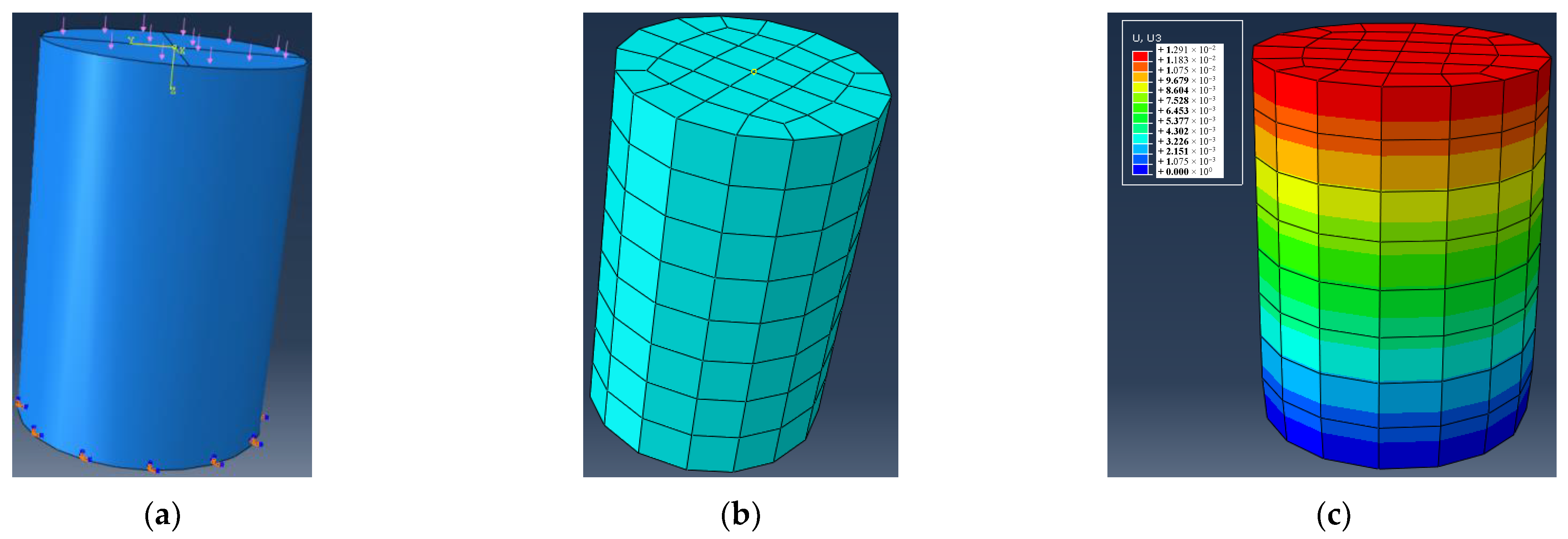
The first step is to determine the size of each component, and the component uses a cylindrical specimen with a diameter of 50 mm × 150 mm. The second step is to determine the structural parameters of the model. The third step is to assemble the components. The fourth step is to set the analysis step, and the viscosity analysis step is adopted in Model 1. The fifth step is load application. A 0.1 MPa uniform load is applied on the cylindrical specimen’s top surface, the cylinder’s bottom is a fixed constraint, and the side is accessible. The sixth step is grid division. The cylinder specimen and the global size of the grid are 20 mm. The finite element calculation model is shown in Figure 3.

3.1. Convergence Analysis

FTS was used to analyze the convergence of the numerical solution. E1 was assumed to be 1560 MPa, μ was assumed to be 0.3, E2 = n1E1, η = n2E1. The influence of time step values on the convergence of the numerical solution under different values of n1 and n2, the fractional order, and calculation time was studied.
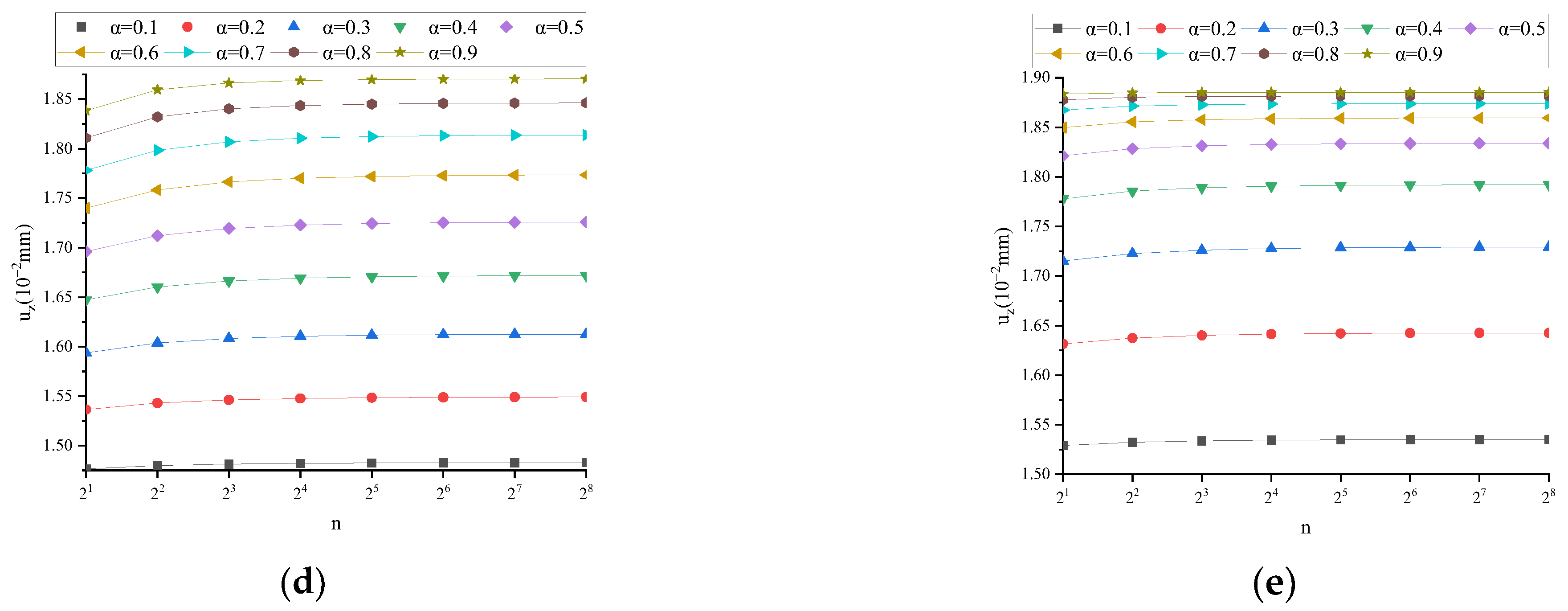
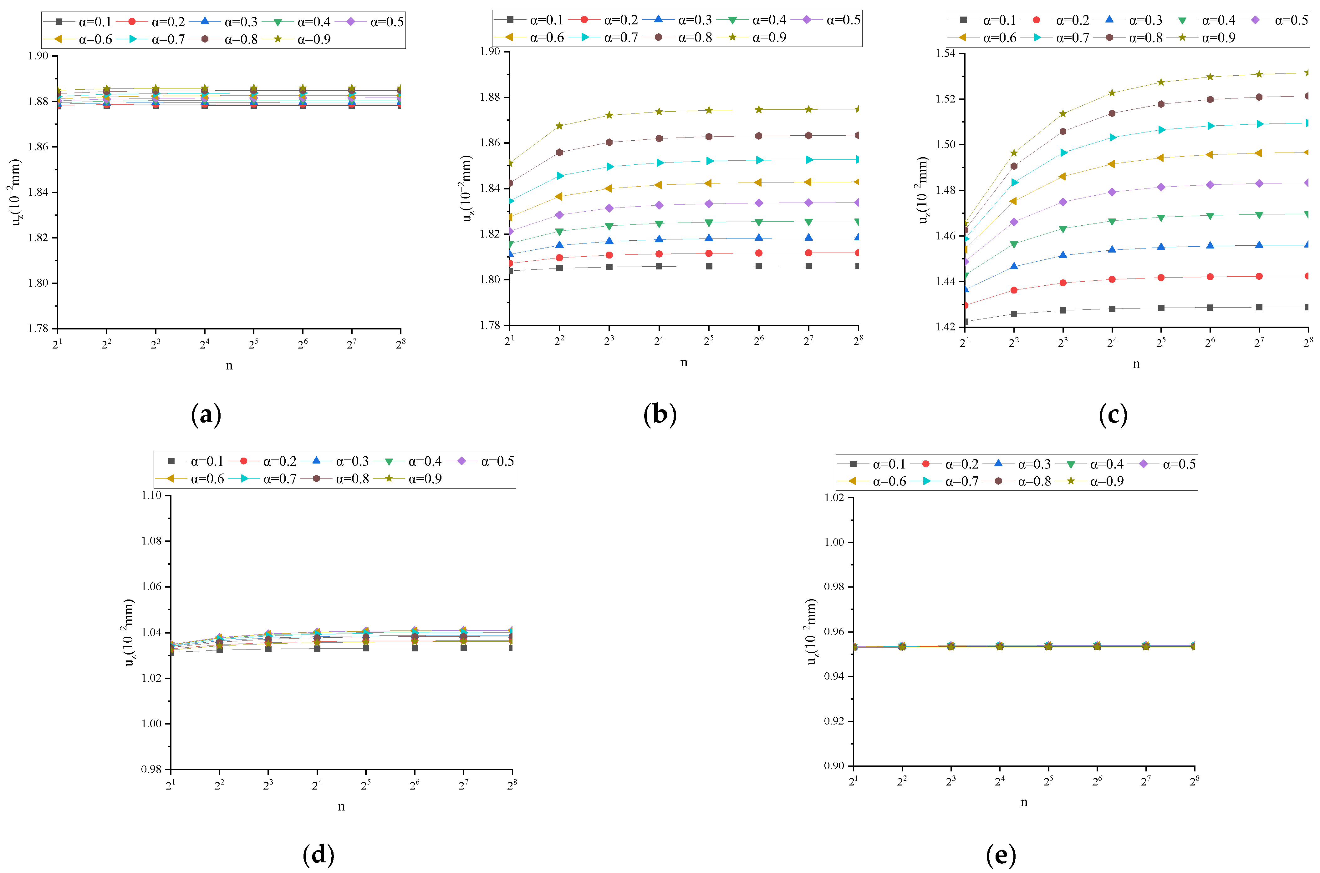
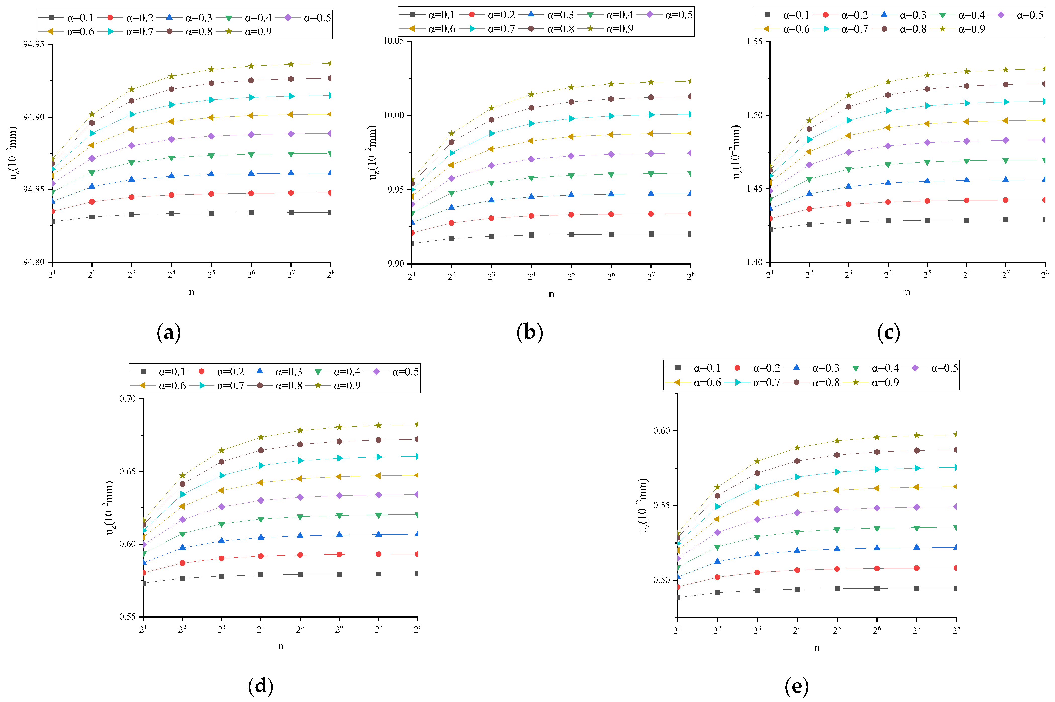
Assuming n1 = 1 and n2 = 1, the vertical displacement of the center of the upper surface of the specimen (uz) in different schedules is calculated. The calculation results are shown in Figure A1. The longitudinal coordinates are of uniform length, the total length is 0.4 × 10⁻² mm, and the scale is 0.05 × 10⁻² mm. As can be seen from Figure A1, when t = 1 s and α = 0.9, it is the most unfavorable state of convergence, and h = t/32 can meet the convergence of two decimal places. Assume n1 = 1 and t = 1 s, and calculate uz different n2 values. The calculation results are shown in Figure A2. The longitudinal coordinates are of uniform length, the total length is 0.12 × 10⁻² mm, and the scale is 0.02 × 10⁻² mm. Figure A2 shows that when n2 = 1 and α = 0.9, it is the most unfavorable state for convergence, and h = t/32 can satisfy convergence to two decimal places. Assuming that n2 = 1 and t = 1 s, uz is calculated under different values of n1. The calculation results are shown in Figure A3. The vertical coordinates are of uniform length, the total length is 0.15 × 10⁻² mm, and the scale is 0.05 × 10⁻² mm. From Figure A3, it can be seen that the value of n1 has almost no effect on convergence. According to the above convergence analysis and calculation results, when t = 1 s and n2 = 1, it is the most unfavorable convergence state, and the larger the α value, the more damaging the convergence. When α = 0.9 and h = t/32, it can meet the intersection after two decimal places. Therefore, when h ≤ t/32 is used for calculating under static load, the results converge when α ≤ 0.9 and other parameters are arbitrary.

3.2. Numerical Solution Verification

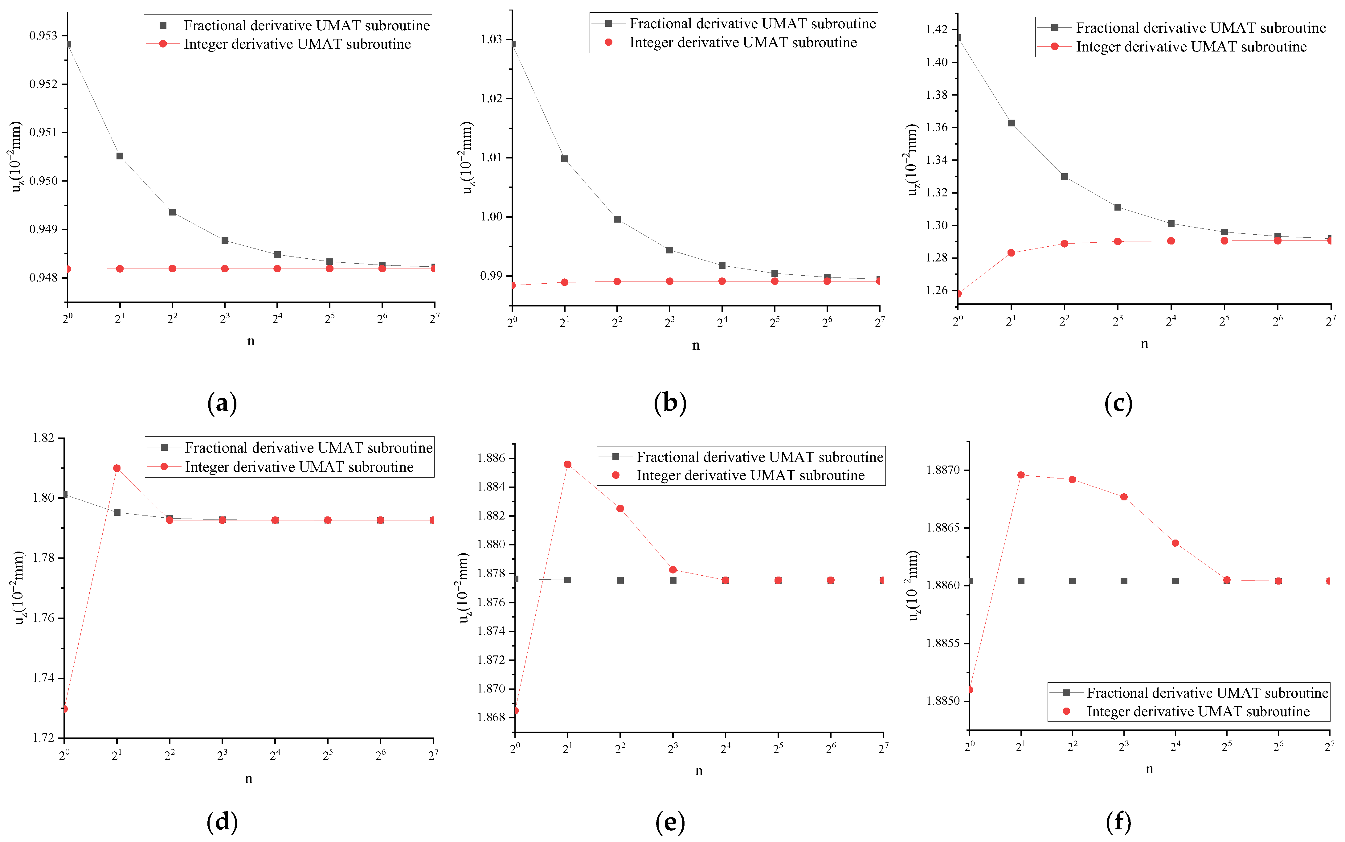
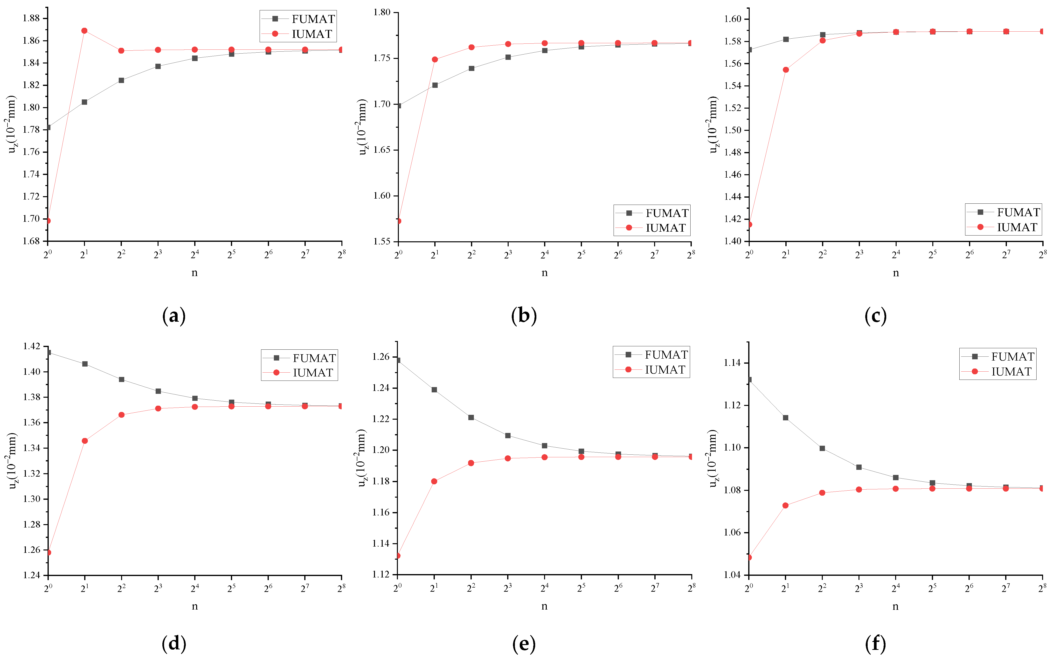
When the fractional derivative UMAT subroutine (FUMAT) α = 1, the calculated results are mutually verified with the integer order UMAT subroutine (IUMAT). Taking uz as an example, the results are shown in Figure 4.
From Figure 4, it can be seen that for the subroutines at the center position of the surface of the cylinder calculated with FUMAT and IUMAT at six different time points, as the number of incremental steps increases, the results calculated with the two tend to be consistent.
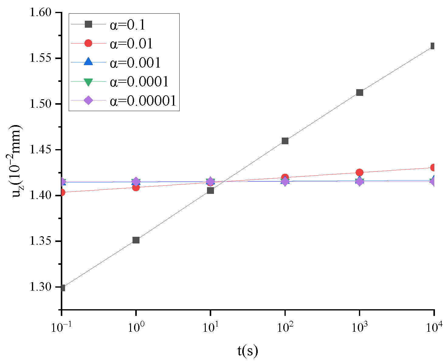
From the definition of the fractional derivative, α cannot be equal to 0. When α tends to 0, taking uz as an example, the calculation results of the fractional derivative viscoelastic and elastic models are shown in Figure 5, and the time step h = 0.01 t is taken. When α = 0, the fractional derivative viscoelastic model degenerates into a linear elasticity model with an elastic modulus of 1040 MPa and Poisson’s ratio of 0.3. In this case, uz = 0.0141523 mm.
Figure 5 shows that when α approaches 0, the vertical displacement time history curve tends toward a straight line, uz = 0.0141523 mm.
When α = 1 and tends to 0, the uz of FTS is consistent with the uz of the three-parameter solid model and linear elasticity model, which proves that the computed results of fractional derivative viscoelasticity in this paper are correct.

3.3. Finite Element Analysis under Several Fractional Derivative and Classical Viscoelastic Models

The dynamic modulus tests of three types of graded rubber-modified asphalt mixtures were conducted using MTS equipment, yielding the dynamic modulus values at various temperatures (15 °C, 30 °C, 45 °C, 60 °C) and loading frequencies (0.1 Hz, 0.5 Hz, 1 Hz, 5 Hz, 10 Hz, 25 Hz). A sigmoid function was employed to establish the primary curve for the dynamic modulus. The dynamic modulus principal curves of rubber-modified asphalt mixtures with three different gradations were fitted using various viscoelastic and fractional derivative viscoelastic models under varying temperatures, and the corresponding fitting results are presented in Table 2 and Table 3.

3.3.1. Several Classical Viscoelastic Models

Taking ARHM-13 as an example, the mechanical response of several classical viscoelastic models is calculated, and the incremental step h is t/50. The uz is shown in Figure 6.
Figure 6 shows that for the Maxwell model, uz tends to infinity as time increases, resulting in distortion. For the classic Kelvin model, when the calculation time is minimal, uz is much smaller than the calculation results of the other two models. Through the comparison of calculation results, it was found that a three-parameter solid model can better describe uz.

3.3.2. Several Fractional Derivative Viscoelastic Models

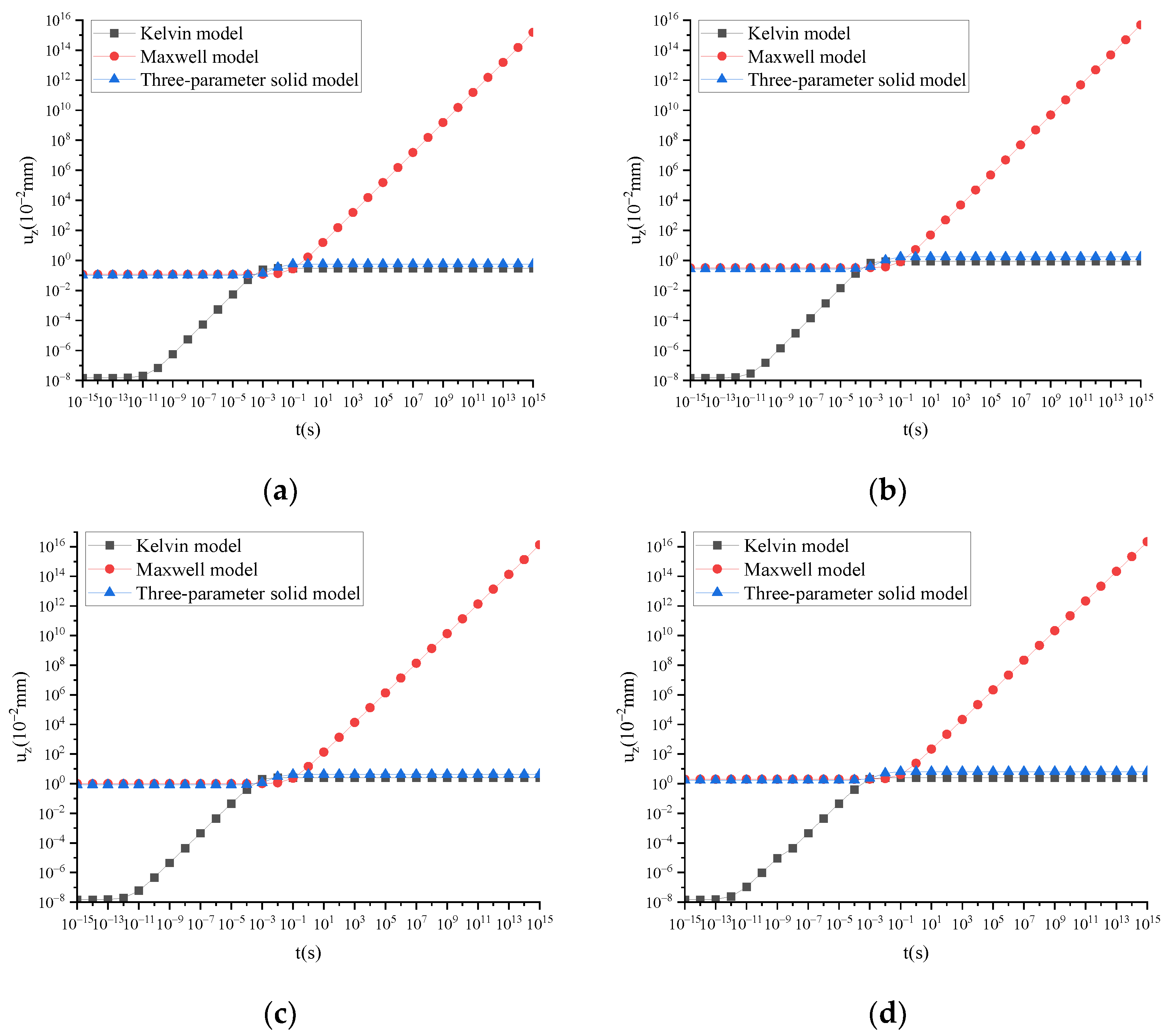
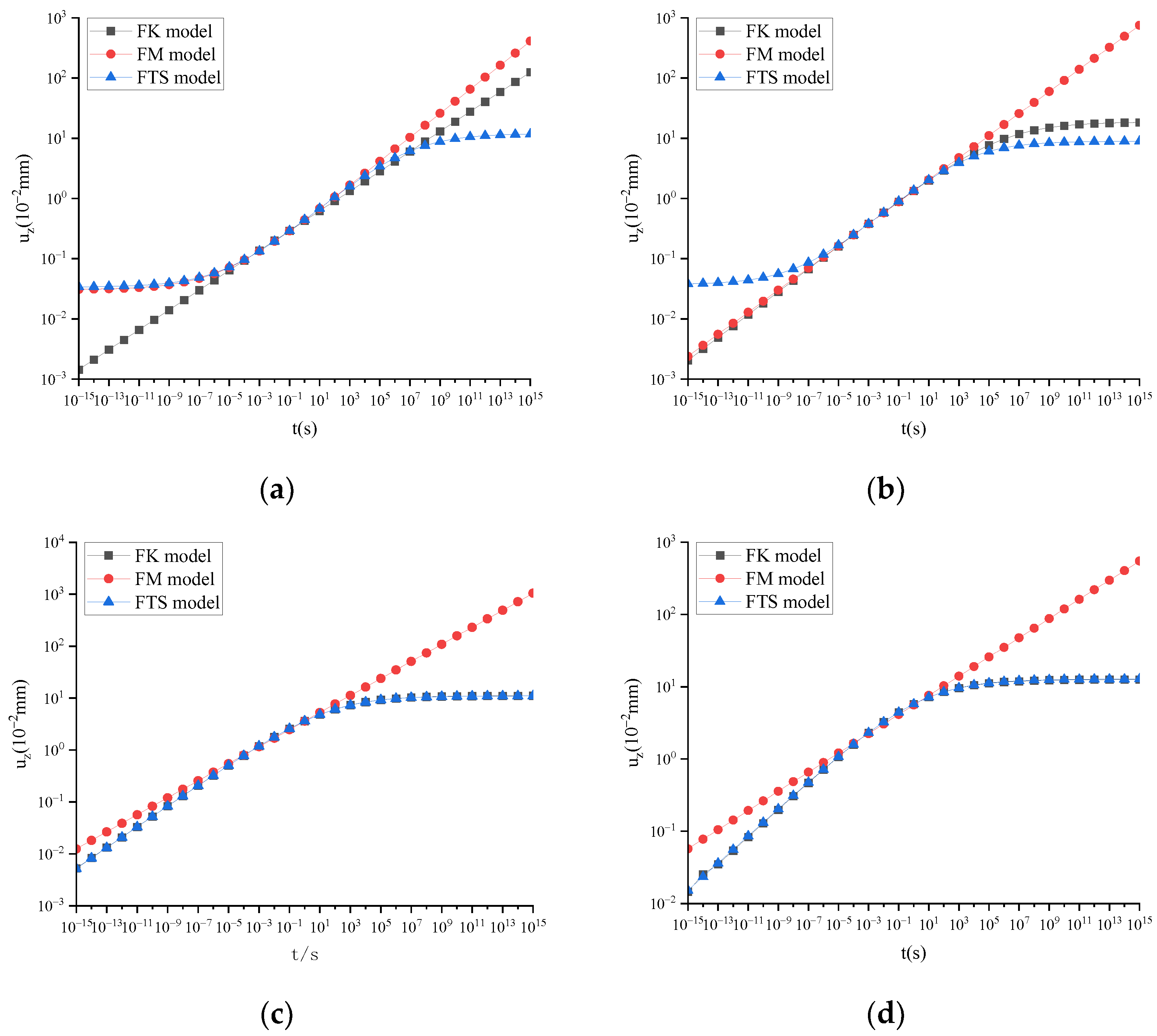
Taking ARHM-13 as an example, the mechanical response of several fractional derivative viscoelastic models is calculated, and the incremental step h is t/50. The uz of several fractional derivative viscoelastic models under different temperatures is shown in Figure 7.
Figure 7 shows that uz tends to infinity for the FM as time increases, resulting in distortion. For the FK, when the calculation time is minimal, uz tends to be 0. Through the comparison of calculation results, it was found that FTS can better describe uz.

3.3.3. FTS and Three-Parameter Solid Model

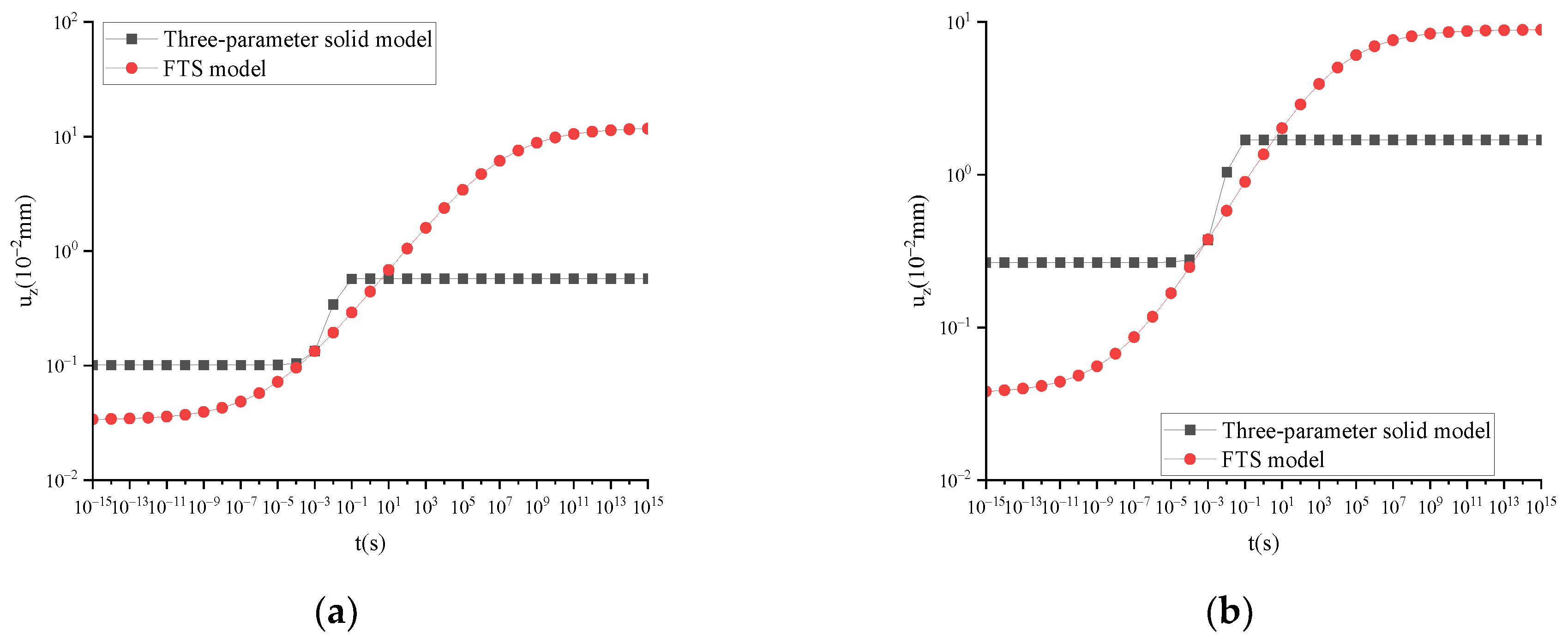
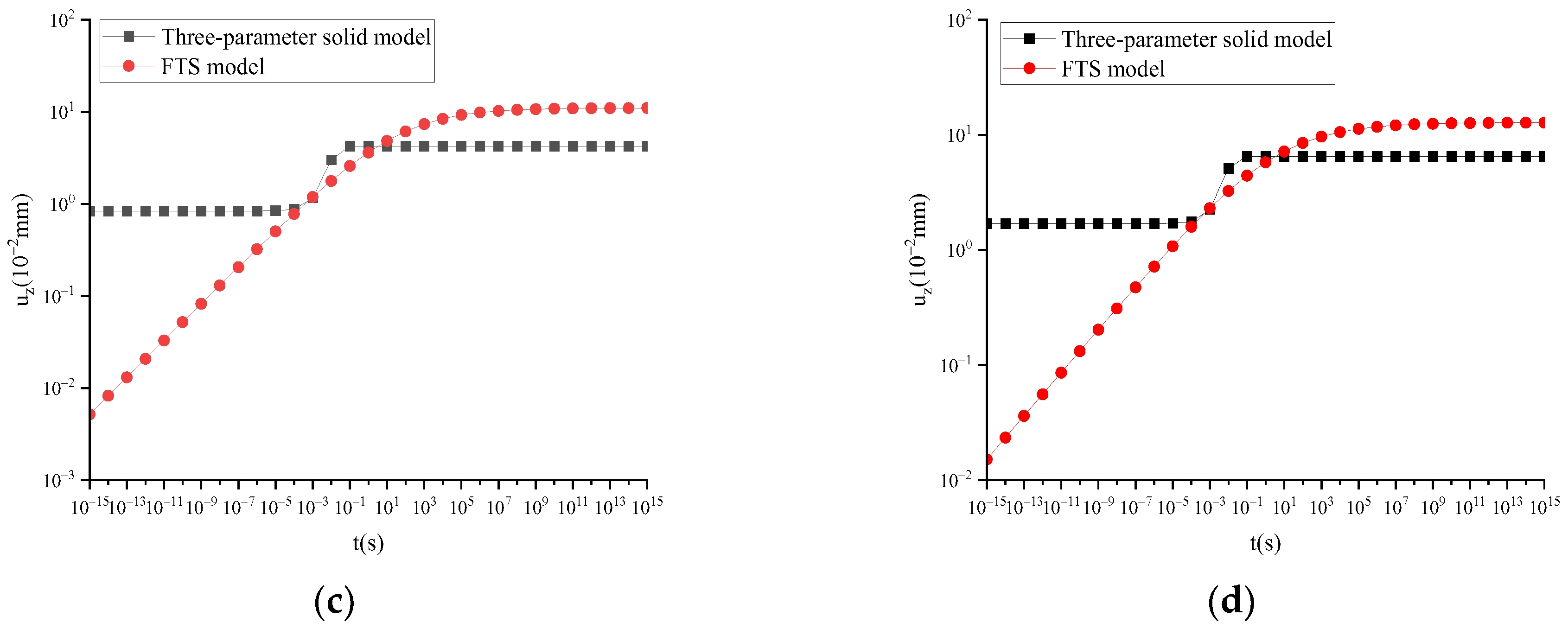
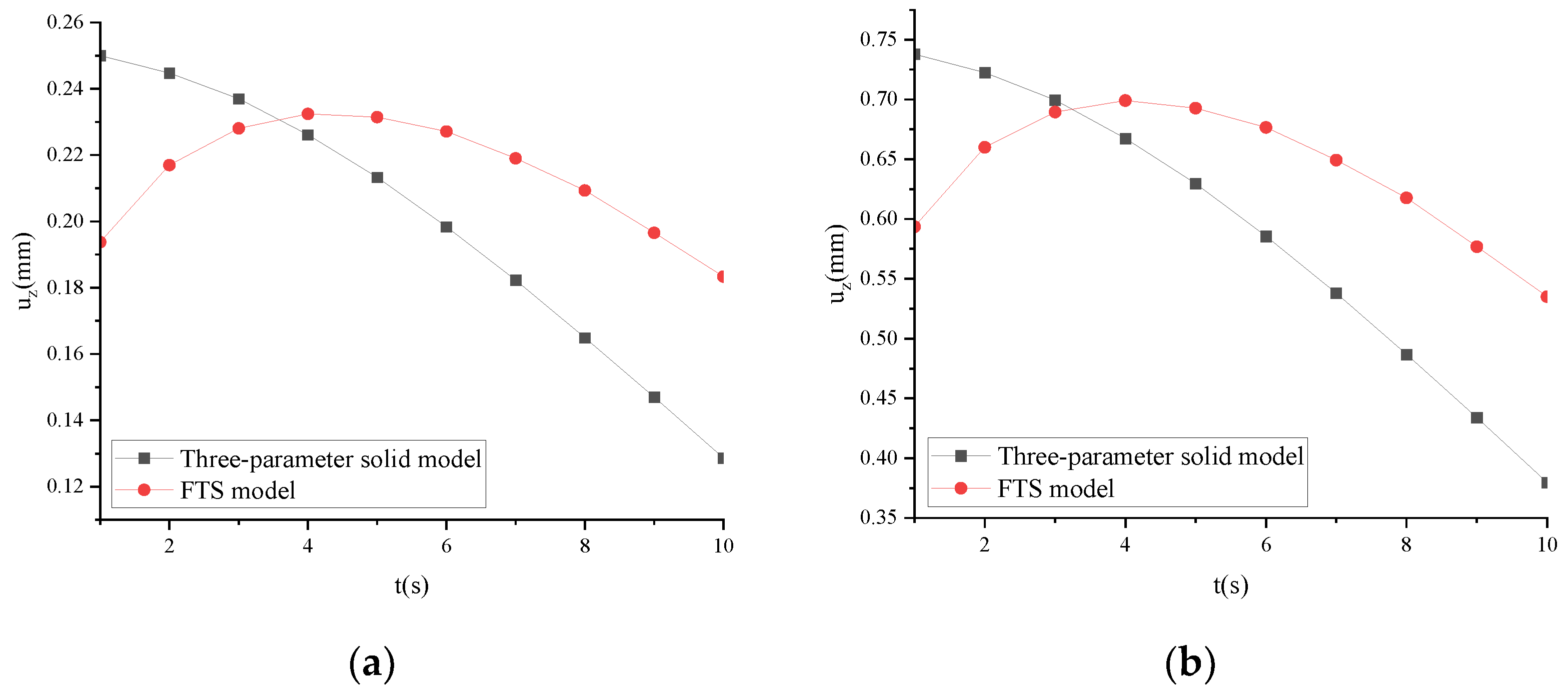
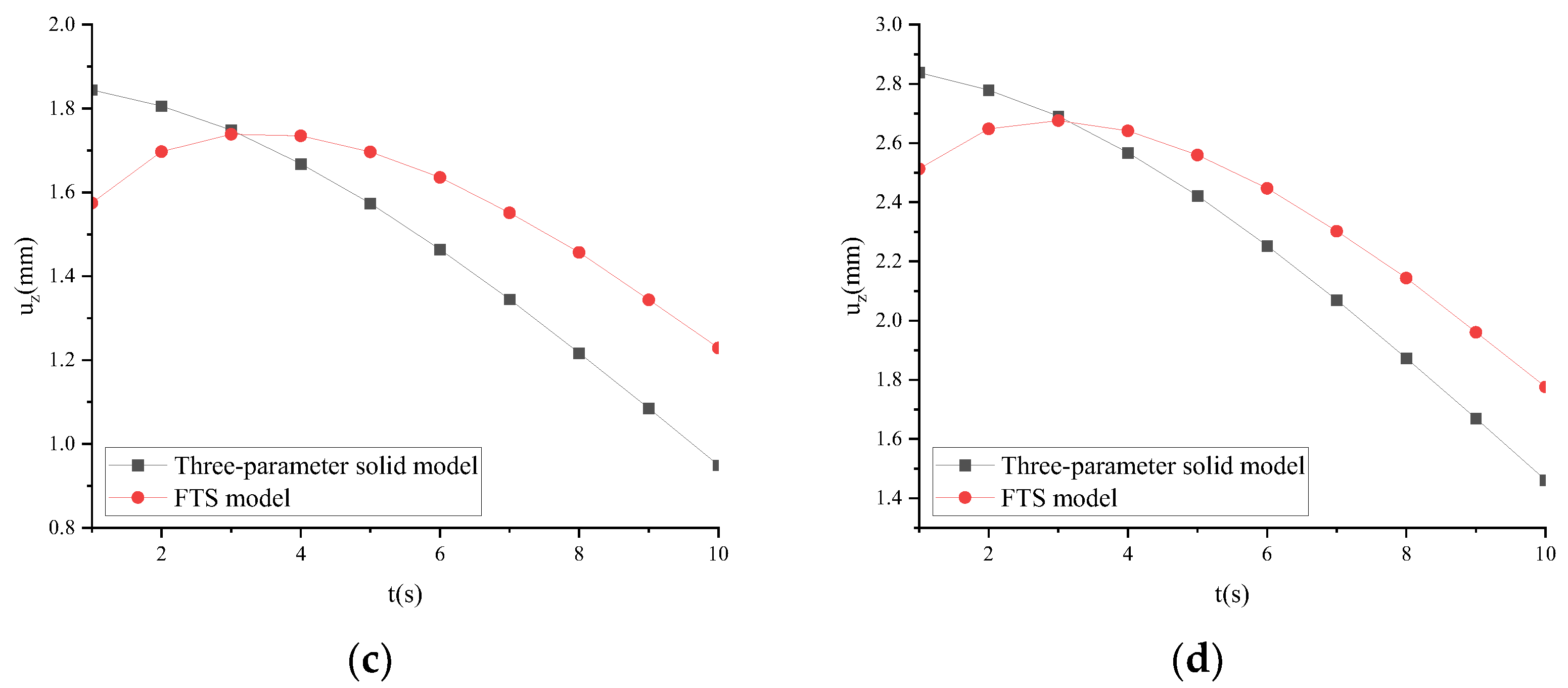
Taking ARHM-13 as an example, the mechanical response of the three-parameter solid model and FTS is calculated, and the incremental step h is t/50. The uz of the three-parameter solid model and FTS under different temperatures is shown in Figure 8.
Figure 8 shows that the vertical displacement curve of the surface center of FTS over time is smoother compared to the three-parameter solid model, which can better describe the displacement characteristics over time and is closer to the actual situation.

3.3.4. FTS under Different Temperatures

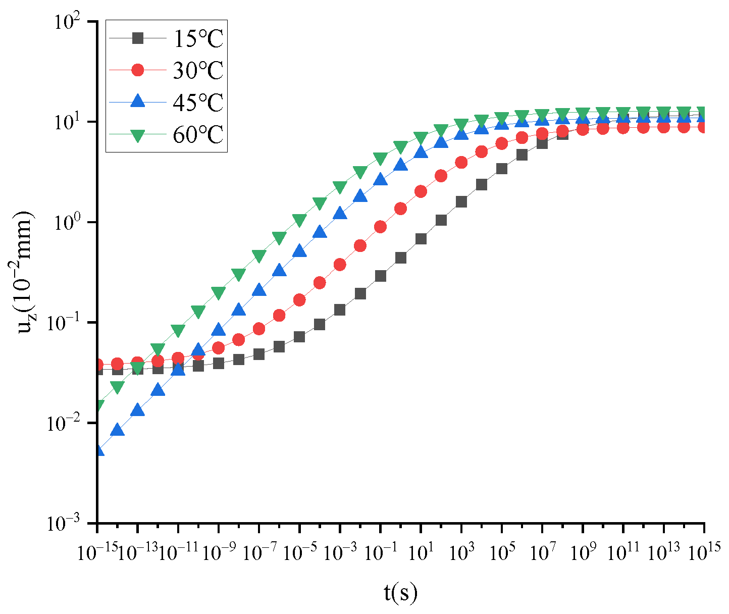
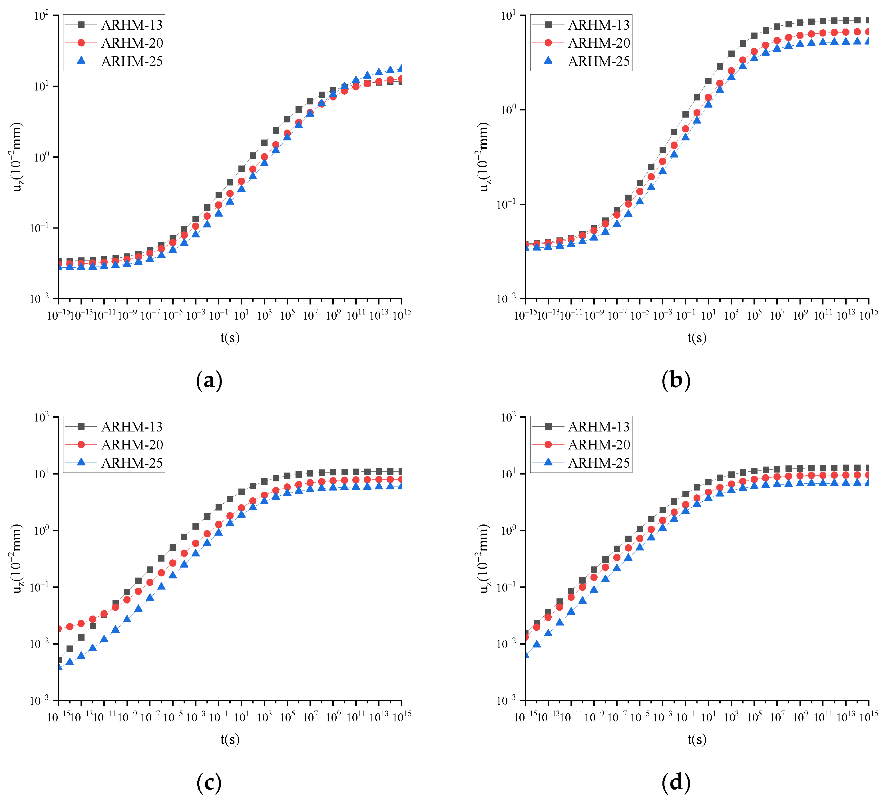
The uz of FTS under different temperatures changes with time, as shown in Figure 9.
The uz increases with temperature in the time interval of 10−10~108 s, as depicted in Figure 9. This observation aligns with the general characteristics of viscoelastic materials, where material stiffness decreases with increasing temperature. However, for t ≤ 10−11 s or t ≥ 109 s, a further increase in temperature no longer leads to an increase in uz. These findings indicate that while FTS provides a better description of viscoelastic properties in rubber-modified asphalt mixtures, subtle differences between this model and the actual constitutive behavior still exist, rendering its application limited across all time domains. Inaccurate results are obtained when calculating extremely small or large timescales.

3.3.5. FTS under Different Gradations

The uz of FTS under different gradations is shown in Figure 10.
The results depicted in Figure 10 demonstrate that within 10−15 s~1015 s, when the temperature reaches or exceeds 30 °C, uz follows a trend of ARHM-25 > ARHM-20 > ARHM-13 as time progresses. Considering the specific applicability range of FTS in the time domain, during the time interval of 10−10~108 s and under all four temperatures, an increasing temporal trend is observed for uz with ARHM-25 > ARHM-20 > ARHM-13.

4. Finite Element Calculation under Dynamic Load

The model described in Section 4.2 is employed, except that a half-sine wave load is utilized instead. Furthermore, the operating area remains consistent with the static load condition. The mathematical expression for the load is presented as follows:
F = p sin 2 π f t
In the formula, p is the load amplitude, 0.1 MPa is taken in this article, and f is the load frequency, 0 t 1 / 2 π f .

4.1. Convergence Analysis

FTS is used to analyze the convergence of the numerical solution. According to the convergence analysis conclusion in Section 2, the convergence is the most unfavorable when n1 = 1. Given that E1 = E2 = 1560 MPa, η = 1560 MPa/s, and μ is 0.3, the influence of the time step on the convergence of numerical solutions under different load frequencies, fractional order, and calculation time is studied.
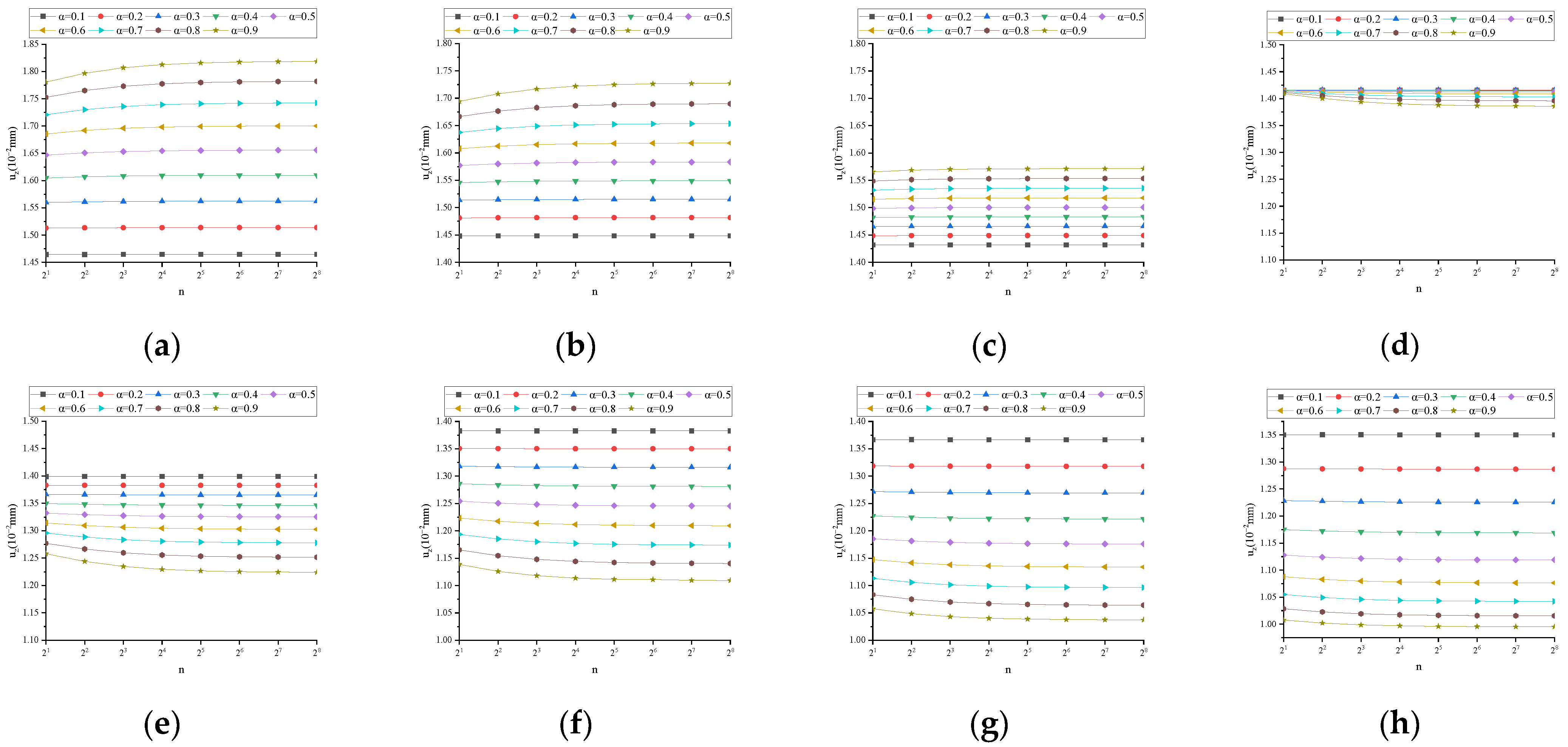
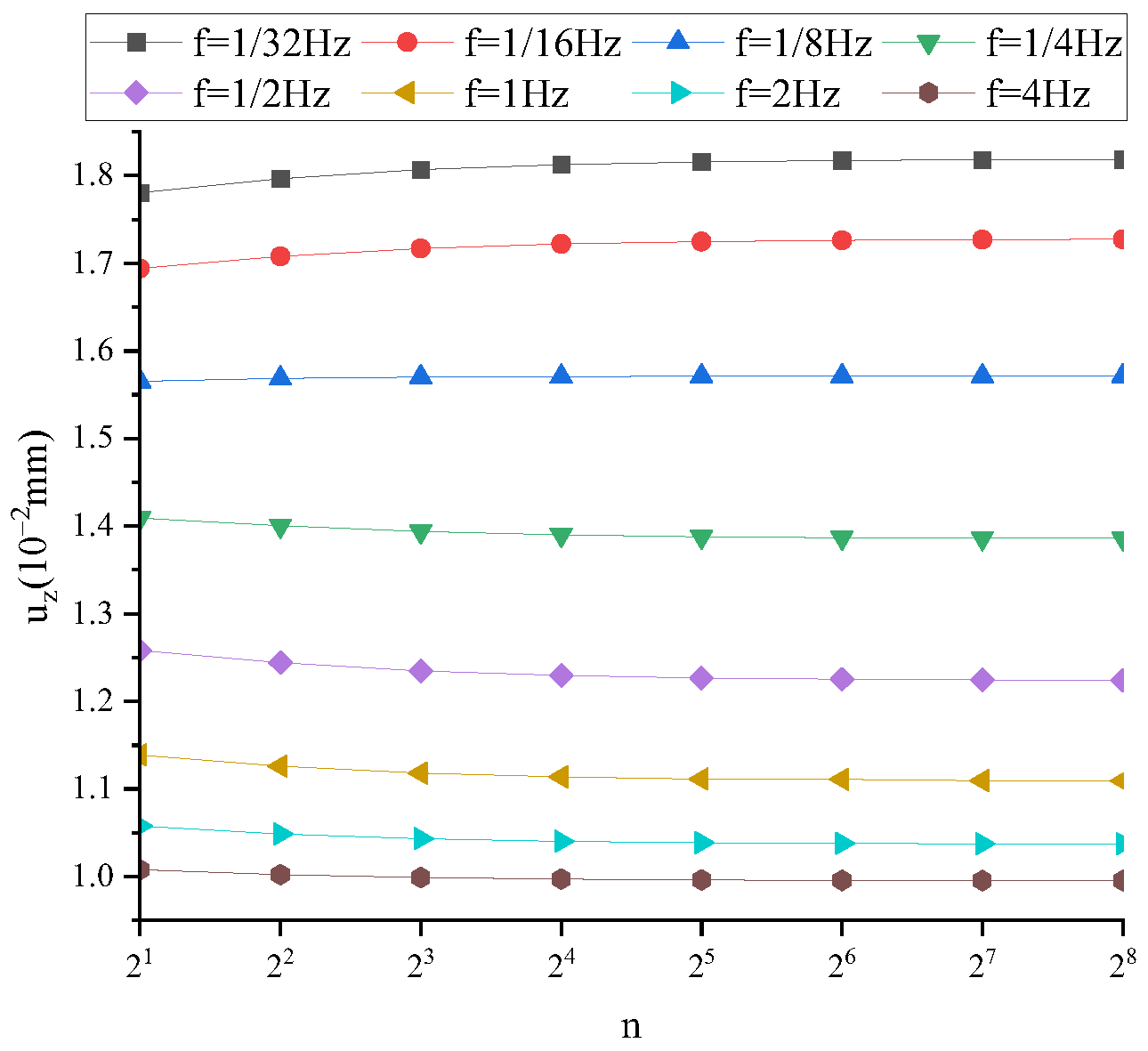
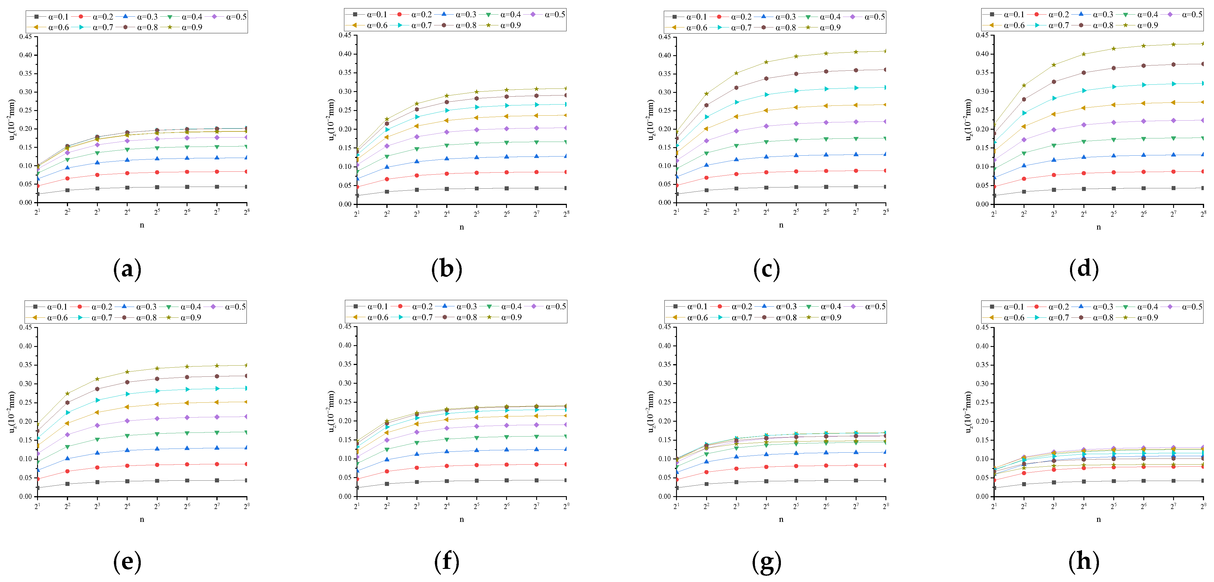
Calculate uz at t = T/4 under different frequency conditions. The calculation results are shown in Figure A4, with a uniform length on the vertical axis and a total length of 0.4 × 10⁻² mm, with a scale of 0.05 × 10⁻² mm. From Figure A4, it can be seen that α = 0.9, which is the most unfavorable state for convergence. When t = T/4 and α = 0.9, uz under different frequency conditions is shown in Figure A5. As can be seen from Figure A5, when h = t/32, convergence after two decimal places can be satisfied. Calculate uz at t = T/2 under different frequency conditions. The calculation results are shown in Figure A6, with a uniform length on the vertical axis and a total length of 0.45 × 10⁻² mm, with a scale of 0.05 × 10⁻² mm. From Figure A6, it can be seen that when α = 0.9, it is the most unfavorable state for convergence. When t = T/2 and α = 0.9, uz under different frequency conditions is shown in Figure A7. From Figure A7, it can be seen that when h = t/128, convergence to two decimal places can be achieved.

4.2. Numerical Solution Verification

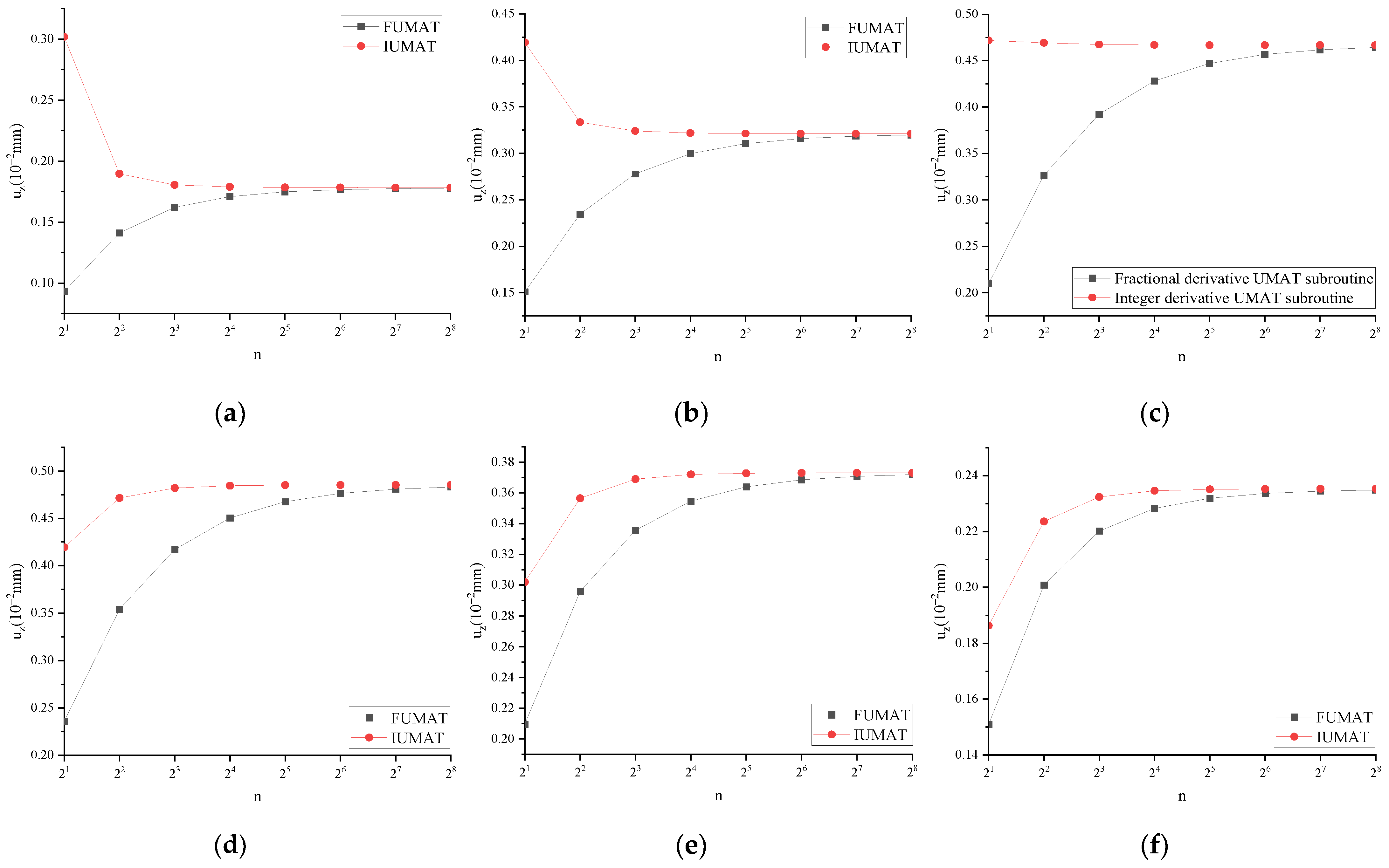
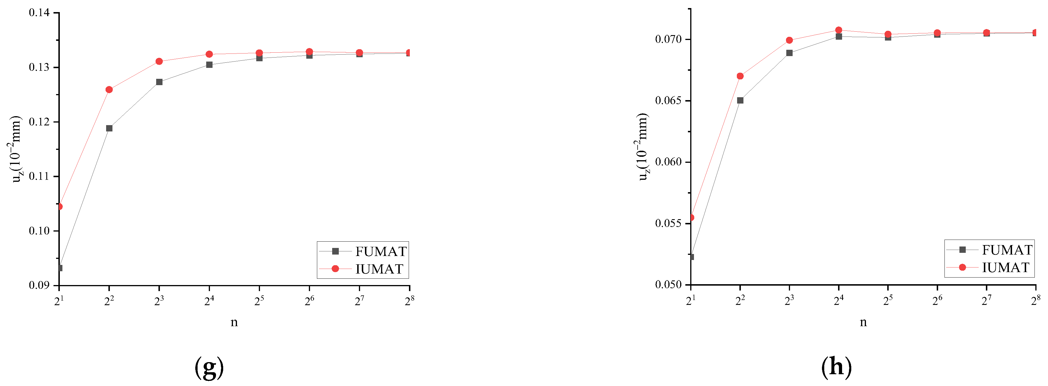
For FUMAT, when α = 1, the calculation results are mutually verified with IUMAT. Taking uz at t = T/4 as an example, the results are shown in Figure 11.
The results from Figure 11 demonstrate that uz, calculated using both FUMAT and IUMAT, tends to exhibit consistency with increasing incremental steps under eight different frequency conditions at t = T/4.
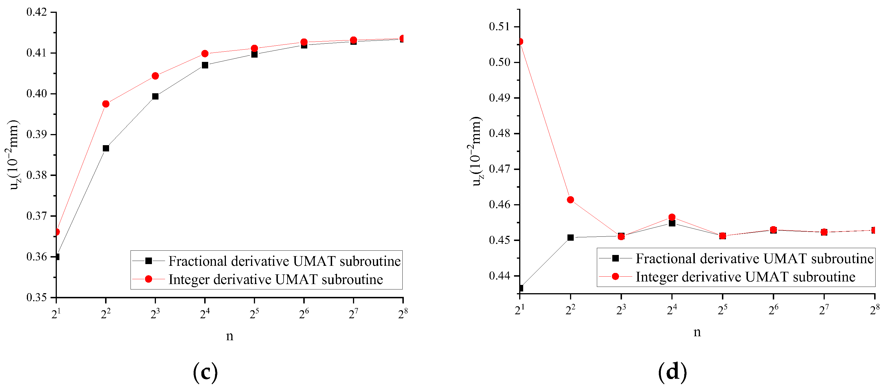
For FUMAT, the calculation results were mutually verified with IUMAT. Taking uz at that time, t = T/4, as an example, the results are shown in Figure 12.
The results from Figure 12 demonstrate that uz, calculated using both FUMAT and IUMAT, tends to exhibit consistency with increasing incremental steps under eight different frequency conditions at t = T/2.
From the definition of the fractional derivative, α cannot be equal to 0. When α tends to 0, taking uz as an example, the calculation results of the fractional derivative viscoelastic and elastic models are shown in Table 4 and Table 5, with the time step h = 0.01 t. When α = 0, the fractional derivative viscoelastic constitutive model degenerates into a linear elasticity model with an elastic modulus of 1040 MPa and Poisson’s ratio of 0.3.
Table 4 and Table 5 show that the closer α approaches 0, the more uz tends toward linear elasticity model calculation results.
When α = 1 and tends to 0, the calculated results are consistent with those of the linear elasticity model and three-parameter solid model, which proves that the results of fractional derivative viscoelastic constitutive calculation in this paper are correct.

4.3. Finite Element Analysis under Several Fractional Derivative and Classical Viscoelastic Models

4.3.1. Several Classical Viscoelastic Models

Taking ARHM-13 as an example, the mechanical response of several classical viscoelastic models is calculated, f = 10 Hz, and the incremental step h is t/128. The uz of several classical viscoelastic models under different temperatures is shown in Figure 13.
Figure 13 shows that the peak value of uz is as follows: three-parameter solid model > Kelvin model > Maxwell model. The occurrence time of the peak value of uz is as follows: three-parameter solid model > Maxwell model > Kelvin model. At the end of load loading, uz is as follows: three-parameter solid model > Maxwell model > Kelvin model.

4.3.2. Several Fractional Derivative Viscoelastic Models

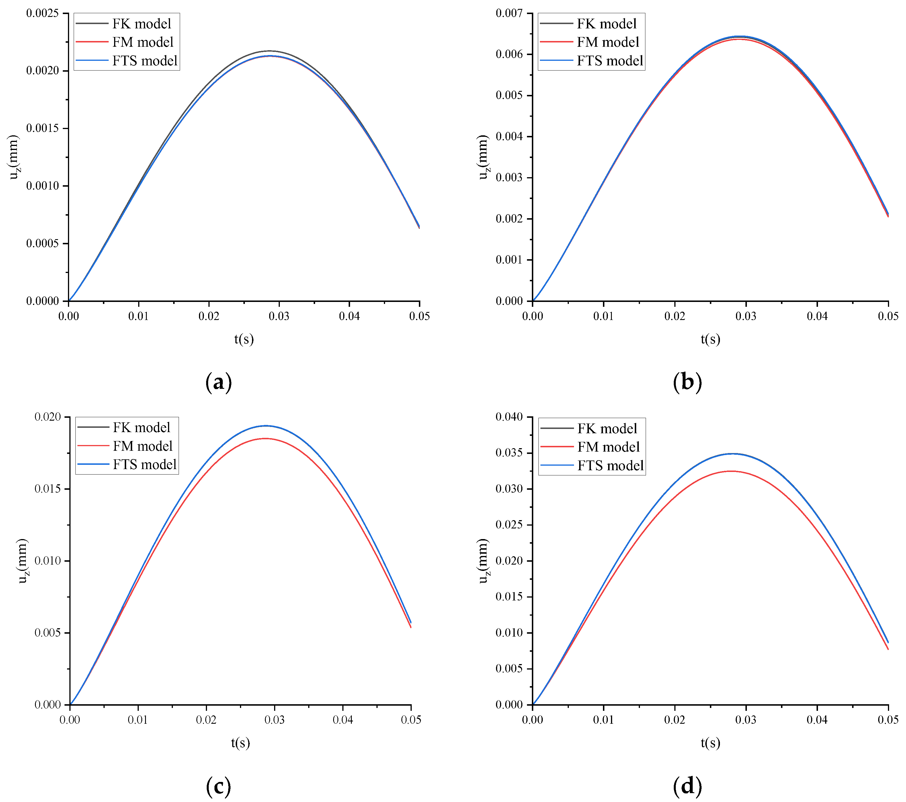
Taking ARHM-13 as an example, the mechanical response of several fractional derivative viscoelastic models is calculated, and the incremental step h is t/128. The uz of several fractional derivative viscoelastic models under different temperatures is shown in Figure 14.
Figure 14 shows that when T = 15 °C, the displacement time curves of the FM and FTS tend to be consistent. The time displacement curve of the FK is higher than that of the FM and FTS. When T ≥ 30 °C, the time displacement curves of the FK and FTS tend to be consistent, and their displacement time curves are higher than those of the fractional order Maxwell model. The higher the temperature is, the more significant the difference is.

4.3.3. FTS and Three-Parameter Solid Model

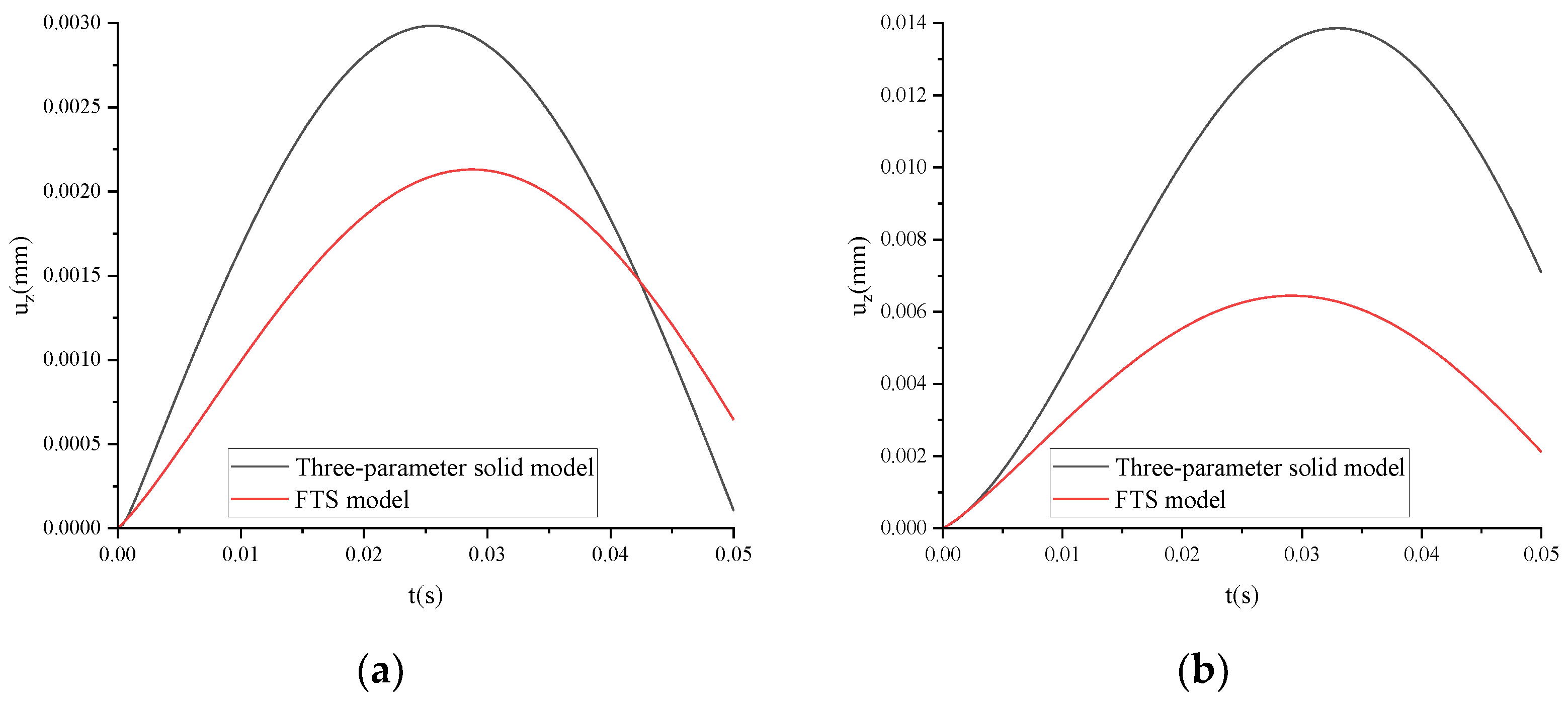
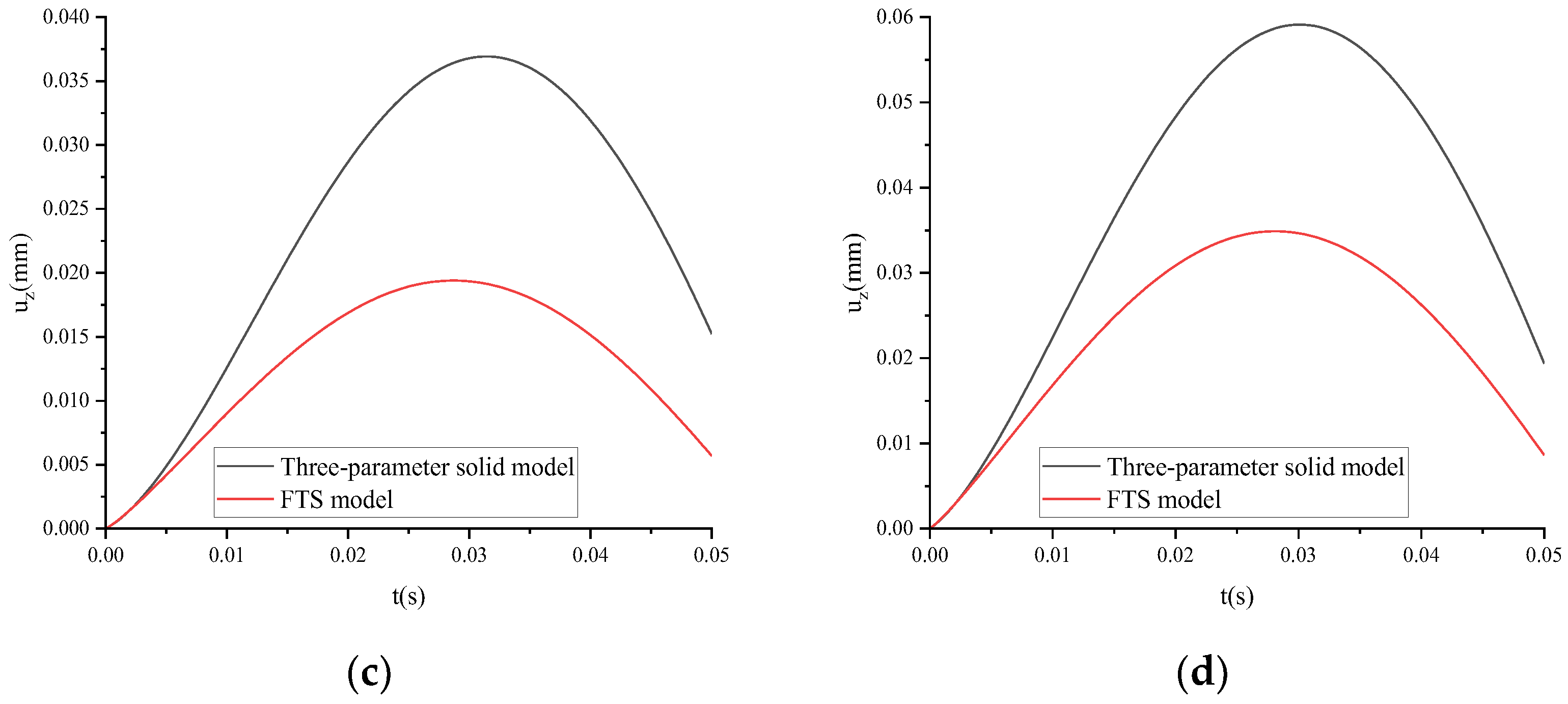
Taking ARHM-13 as an example, the mechanical response of the three-parameter solid model and FTS is calculated, and the incremental step h is t/128. uz of the three-parameter solid model and FTS under different temperatures is shown in Figure 15.
From Figure 15, it can be seen that the peak value of uz is as follows: the three-parameter solid model > FTS. When the peak value of uz occurs at T = 15 °C, FTS > three-parameter solid model; when T ≥ 30 °C, the three-parameter solid model > FTS. At the end of load loading, uz, when T = 15 °C, is as follows: FTS > three-parameter solid model. When T ≥ 30 °C, the three-parameter solid model > FTS.

4.3.4. FTS under Different Temperatures

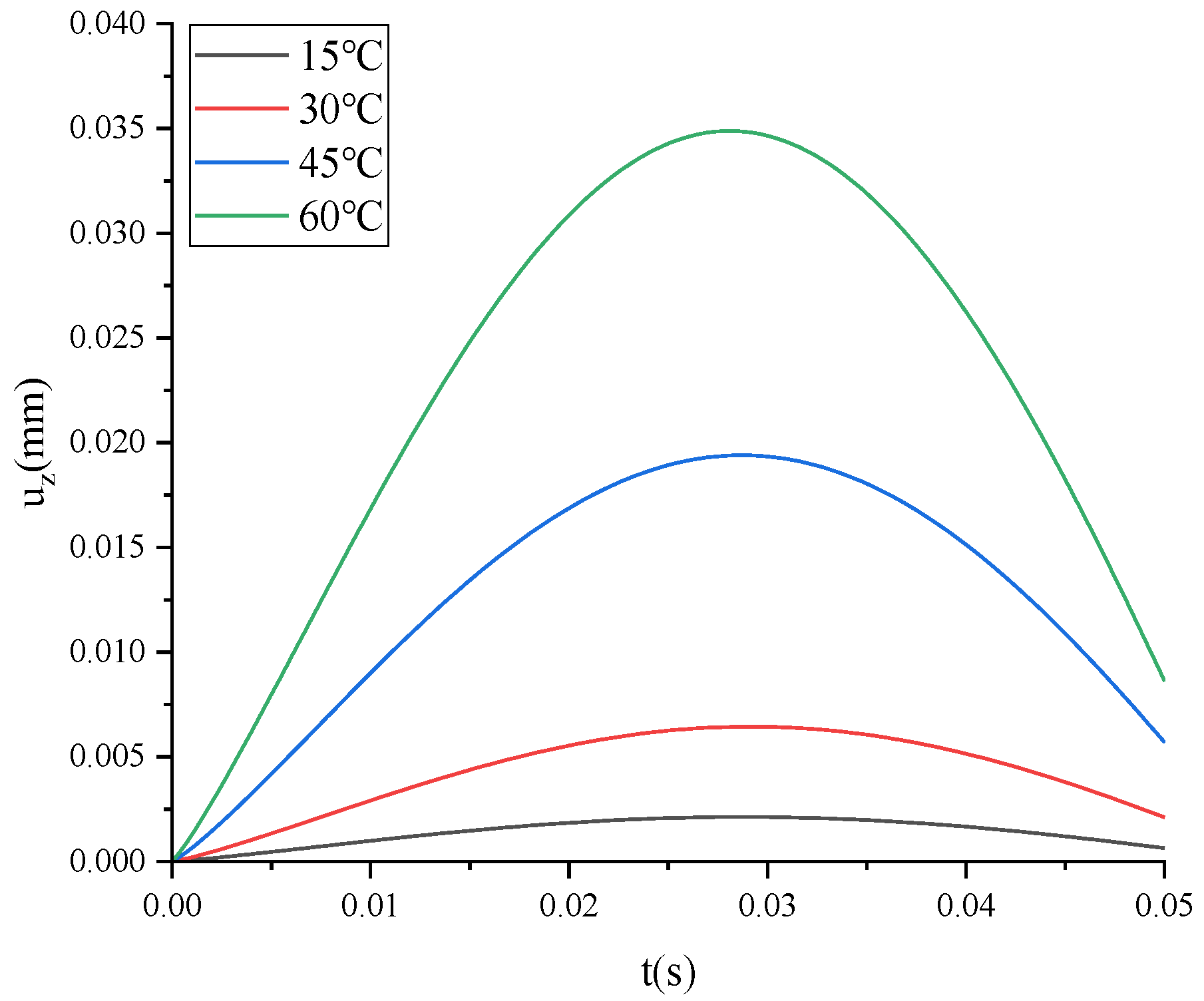
uz of FTS under different temperatures changes with time, as shown in Figure 16.
As shown in Figure 16, the higher the temperature, the larger the peak value of uz, and the later the peak value of uz. At the end of loading, the higher the temperature is, the greater uz is.

4.3.5. FTS under Different Gradations

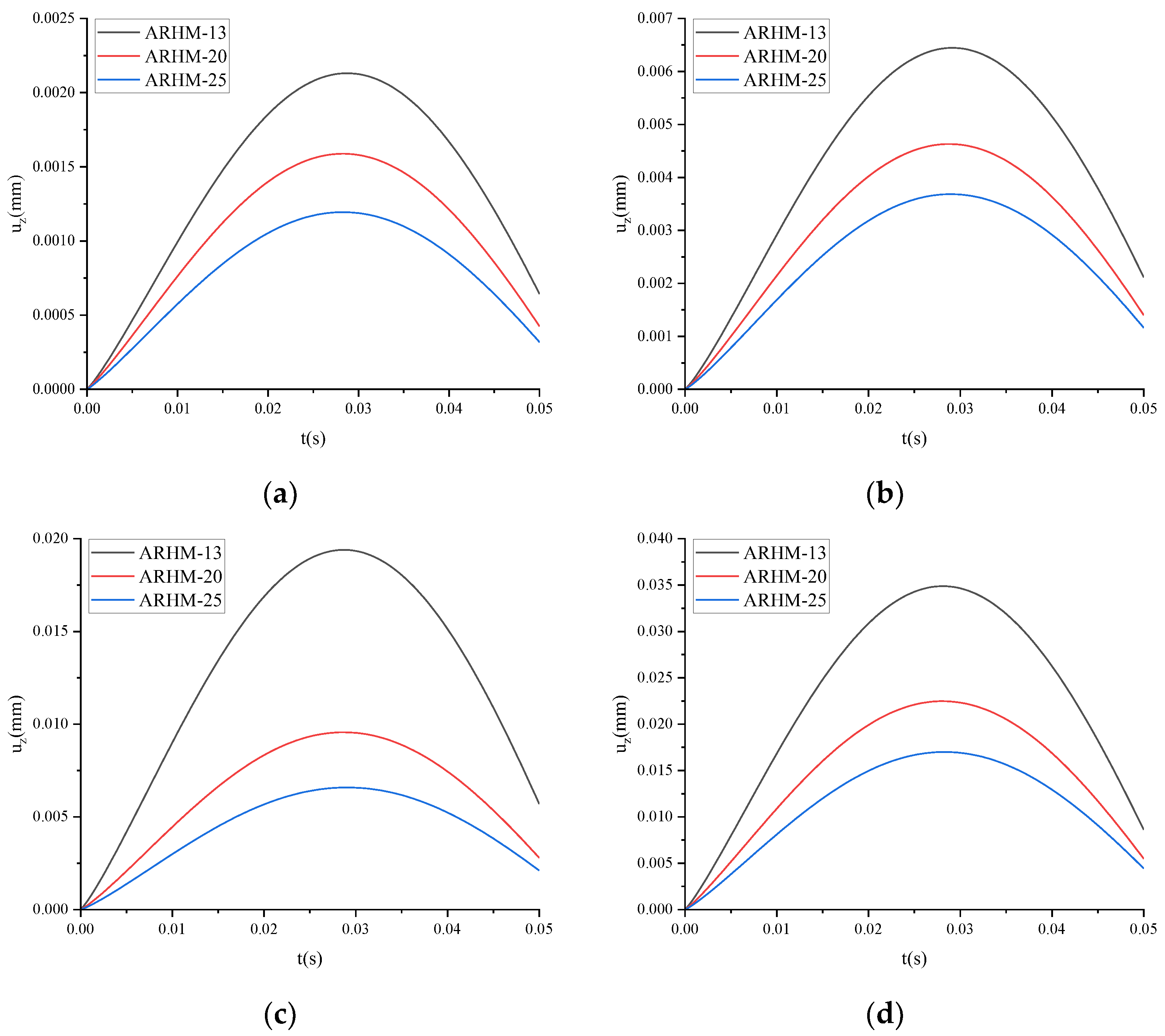
uz of the FTS under different gradations is shown in Figure 17.
As can be seen from Figure 17, the peak value of uz, the time when the peak value of uz occurs, and uz at the end of loading are as follows: ARHM-13 > ARHM-20 > ARHM-25.

5. Finite Element Calculation under Moving Load

The first step is to determine the size of each component. The component is a beam specimen with a length of 1000 mm, a width of 100 mm, and a height of 100 mm. The second step is to determine the structural parameters of the model. The third step is to assemble the components. The fourth step is to set the analysis step, and the model adopts the viscosity analysis step. The fifth step is load application. The moving load of a 100 mm × 100 mm square with the size of 0.1 MPa is applied to the beam specimen’s top surface. The velocity remains constant. The beam specimen and the two ends of the beam specimen are fixed constraints. The sixth step is grid division. The global grid size used for the cylinder specimen is 50 mm. The finite element calculation model is shown in Figure 18.

5.1. Convergence Analysis

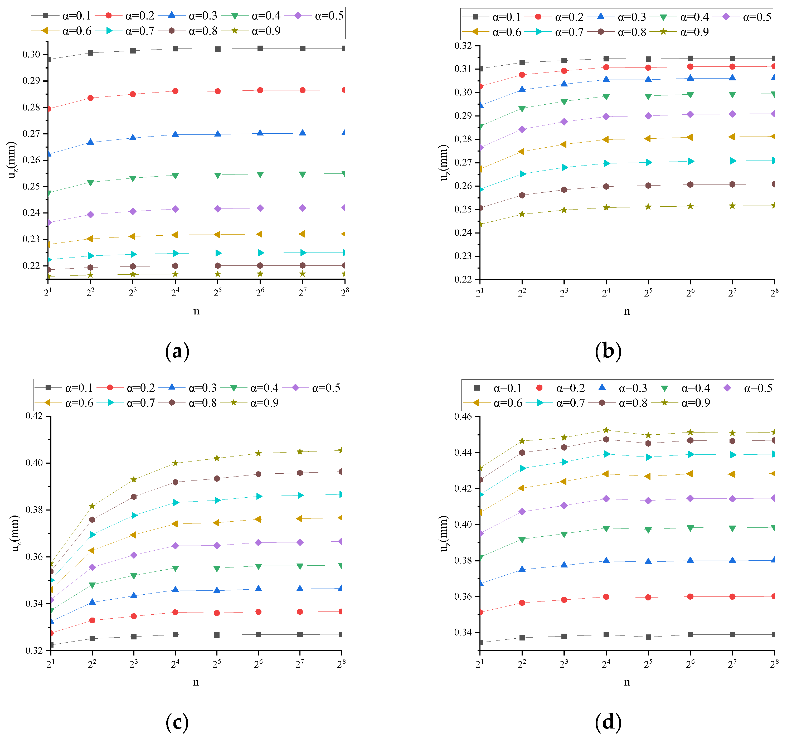
The convergence analysis of numerical solutions was conducted using FTS. From the convergence analysis conclusion in Section 2, it can be seen that the convergence is most unfavorable when n1 = 1. Assume that E1 = E2 = 1560 MPa, η = 1560 MPa/s, μ = 0.3. Taking the example of moving a load to a distance of 1/4 of the beam span from the edge, this study investigates the convergence of vertical displacement at the center of the bottom surface (ω). Under different working conditions, ω is shown in Figure A8. Figure A8 shows that when v = 250 mm/s and t = 1 s, it is the most unfavorable state for convergence; h = t/256 can satisfy convergence to two decimal places. Like under static load, when t = 1 s, it is the most unfavorable state for convergence.

5.2. Numerical Solution Verification

For FUMAT, when α = 1, the calculation results are mutually verified with IUMAT. Taking ω as an example, ω under different working conditions of FUMAT and IUMAT subroutines is shown in Figure 19.
Figure 19 shows that for ω of FUMAT and IUMAT under four different operating conditions, the results calculated with the two subroutines tend to be consistent with the increase in incremental steps.
From the definition of the fractional derivative, α cannot be equal to 0. When α tends to 0, taking ω as an example, the calculation results of the fractional derivative viscoelastic and elastic models are shown in Table 6, and the time step h = t/256 is taken. When α = 0, the fractional derivative viscoelastic constitutive model degenerates into a linear elasticity model with an elastic modulus of 1040 MPa and Poisson’s ratio of 0.3.
As can be seen from Table 6, when α tends to 0, ω tends to be the calculation result of the linear elasticity model.
When α is equal to 1 and tends to 0, the calculated results are consistent with those of the linear elasticity model and three-parameter solid model, which proves that the calculated results of fractional derivative viscoelasticity in this paper are correct.

5.3. Finite Element Analysis under Several Fractional Derivative and Classical Viscoelastic Models

5.3.1. Several Classical Viscoelastic Models

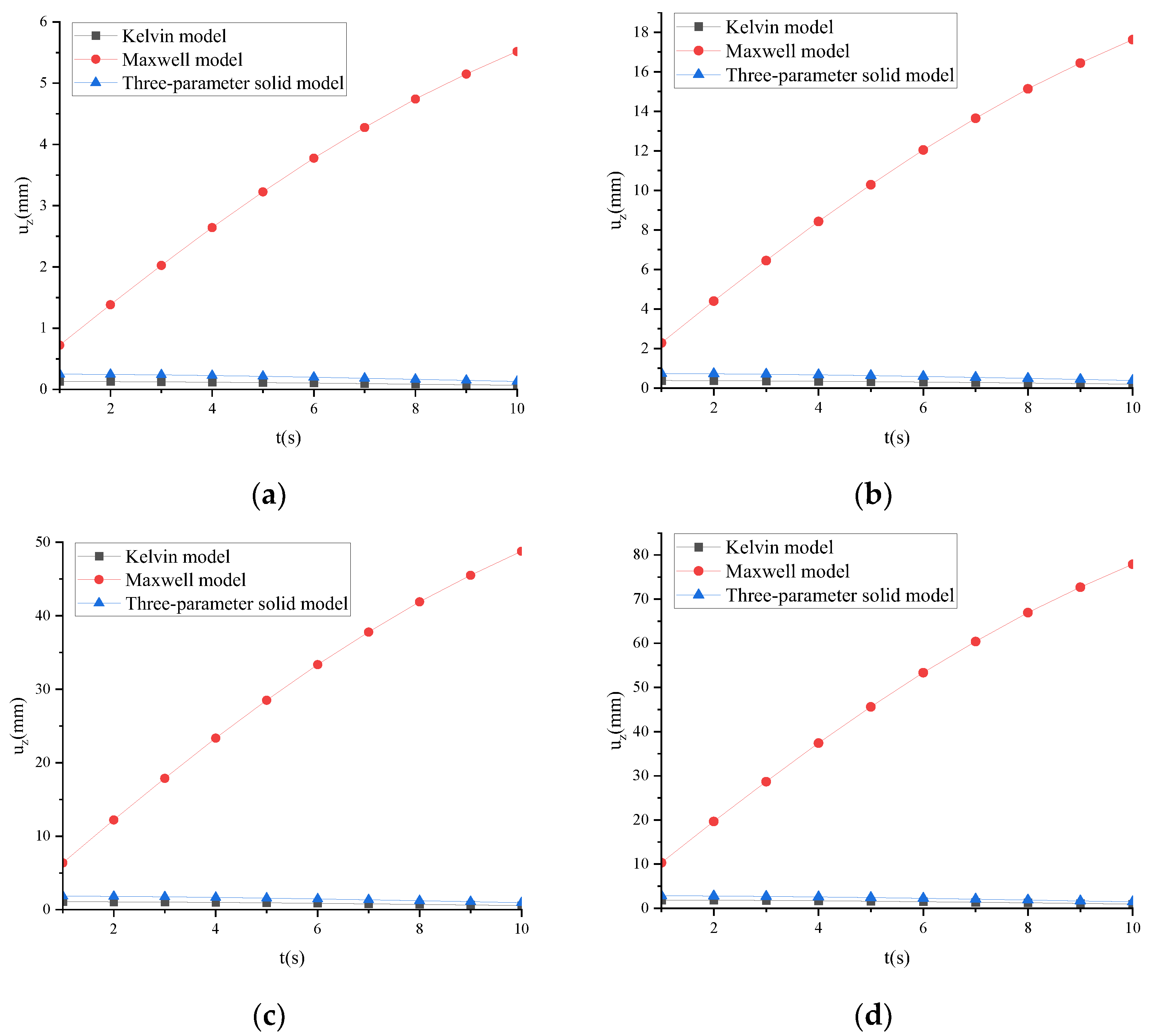
Taking ARHM-13 as an example, the mechanical response of several classical viscoelastic models is calculated, and the incremental step h is t/256. v = 25 mm/s and t = 10 s. ω of several classical viscoelastic models under different temperatures is shown in Figure 20.
Figure 20 shows that as the loading time increases, for the Maxwell model, ω increases linearly with time, resulting in distorted results. The Kelvin model and the three-parameter solid model show that ω slowly decreases with time, and the displacement is relatively small. Compared with the Maxwell model, they can better describe the actual state of the beam.

5.3.2. Several Fractional Derivative Viscoelastic Models

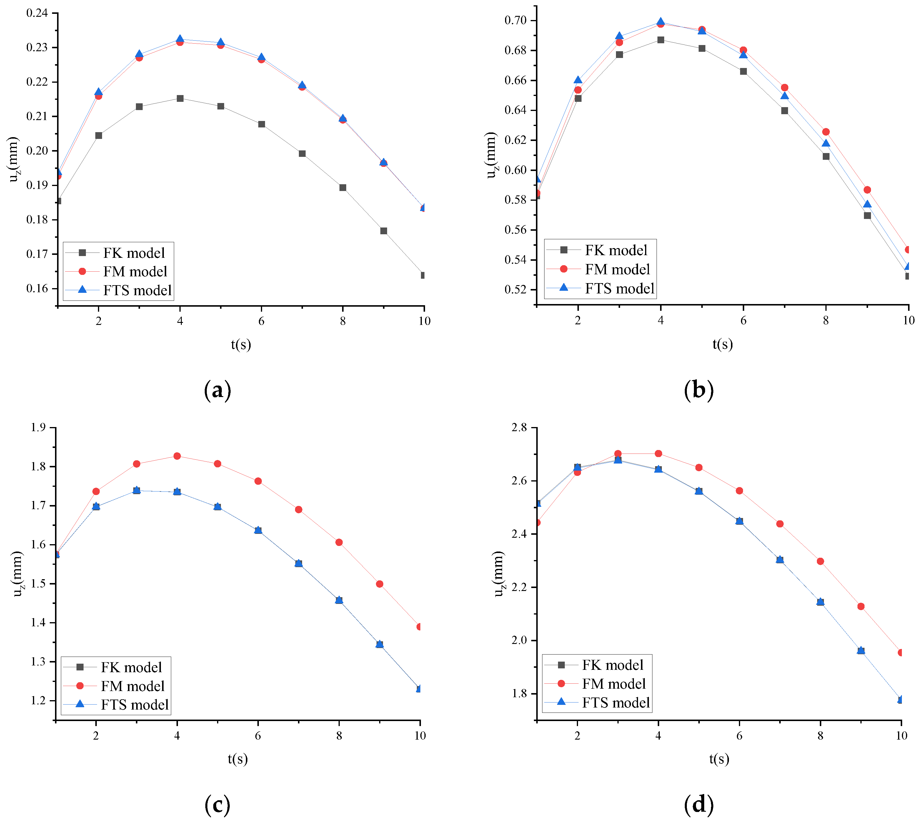
Taking ARHM-13 as an example, the mechanical response of several fractional derivative viscoelastic models is calculated, and the incremental step h is t/256. v = 25 mm/s and t = 10 s. ω of several fractional derivative viscoelastic models under different temperatures is shown in Figure 21.
Figure 21 shows that when T ≤ 30 °C, the results of FM and FTS are closer, and the lower the temperature, the closer the two results are. When T ≥ 45 °C, the FK is closer to FTS.

5.3.3. FTS and Three-Parameter Solid Model

Taking ARHM-13 as an example, the mechanical response of the three-parameter solid model and FTS is calculated, and the incremental step h is t/256. v = 25 mm/s and t = 10 s. ω of the three-parameter solid model and FTS under different temperatures is shown in Figure 22.
Figure 22 shows that in the initial stage of load action, ω is as follows: three-parameter solid model > FTS. As the action time increases, ω is as follows: FTS > three-parameter solid model.

5.3.4. FTS under Different Temperatures

ω of FTS under different temperatures is shown in Figure 23.
As can be seen from Figure 23, ω is as follows: 60 °C > 45 °C > 30 °C > 15 °C. The higher the temperature is, the more obvious ω is.

5.3.5. FTS under Different Gradations

ω of FTS under different gradations is shown in Figure 24.
As can be seen from Figure 24, the vertical displacement in the middle of the beam span is as follows: ARHM-13 > ARHM-20 > ARHM-25. The maximum time of vertical displacement is about 4 s.

6. Conclusions

The present study presents a methodology for implementing the computation of a three-dimensional fractional derivative viscoelastic model within the finite element framework, utilizing the commercial finite element software ABAQUS external subprogram UMAT. Three distinct loading conditions, namely static load, dynamic load, and mobile load, are individually analyzed and computed. Furthermore, classical and fractional derivative viscoelastic rubber-modified asphalt mixture models are examined and calculated. The key findings are as follows:
(1) In the convergence analysis of static load, dynamic load, and mobile load models in this paper, when the fractional order is 0.1 ≤ α ≤ 0.9, the incremental step h is set as t/32, t/128, and t/256, respectively, to satisfy the two-digit convergence requirements. The selection of the incremental step depends on various factors, including the model type, load characteristics, and fractional order. During calculation, a trial method can be employed to determine an appropriate value for h while ensuring computational accuracy. It is advisable to use a more giant incremental step whenever possible to reduce computational workload.
(2) FK and Kelvin models are fundamentally solid, which may introduce inaccurate calculation results when the computation time is short. Similarly, the FM and Maxwell models are essentially liquid models, which can also lead to distortions in calculation results when the computation time is extended. FTS possesses the combined advantages of FK and FM, enabling an accurate depiction of material viscoelastic characteristics across a broad time spectrum.
(3) In current pavement mechanics calculations, the mechanical analysis of an asphalt mixture commonly relies on either the linear elasticity model or the classical viscoelasticity model, resulting in disparities between calculated results and real-world scenarios. Therefore, it is imperative to comprehensively consider the fractional derivative viscoelastic characteristics of an asphalt mixture during calculations.
(4) This article’s simulation method applies to viscoelastic materials with the dynamic modulus varying with load frequency and temperature, similar to asphalt mixtures. Different viscoelastic materials may be suitable for different fractional derivative viscoelastic models, which requires obtaining the fractional derivative viscoelastic model used through experiments and a constitutive analysis. The method in this article can be referred to for an analysis and calculation.
(5) Due to the limited computing storage space of ABAQUS, implementing the fractional derivative viscoelastic model in a finite element analysis requires that the stress and strain data generated during calculations should be at most 2 GB. This limitation imposes constraints on the model’s size and the number of incremental steps. Consequently, implementing a multi-grid, multi-incremental step fractional derivative viscoelastic finite element model becomes challenging within this framework. However, future computer computing power advancements and commercial finite element software updates are expected to facilitate such implementations.

Author Contributions

Conceptualization: S.L.; methodology: G.Z.; validation: G.Z. and N.Z.; formal analysis: S.L. and G.Z.; investigation: S.L. and N.Z.; resources: N.Z.; data creation: S.L. and G.Z.; writing: N.Z. and G.Z.; writing—review and editing: N.Z. and G.Z.; visualization: N.Z. and G.Z.; supervision: N.Z.; project administration: G.Z.; funding acquisition: S.L. All authors have read and agreed to the published version of the manuscript.

Funding

This work was supported by National Natural Science Foundation of China (52225806 and 52078063) and Open Fund of Key Laboratory of Special Environment Road Engineering of Hunan Province (kfj230602).

Data Availability Statement

The data analyzed in this study are subject to the following licenses/restrictions: the first author can receive the restrictions. Requests to access these datasets should be directed to [email protected].

Conflicts of Interest

Authors declare no conflicts of interest.

Appendix A

Figure A1. uz (n1 = 1, n2 = 1): (a) t = 0.01 s; (b) t = 0.1 s; (c) t = 1 s; (d) t = 10 s; (e) t = 100 s.
Fractalfract 08 00103 g0a1aFractalfract 08 00103 g0a1b
Figure A2. uz (n1 = 1, t = 1 s): (a) n2 = 0.01; (b) n2 = 0.1; (c) n2 = 1; (d) n2 = 10; (e) n2 = 100.
Fractalfract 08 00103 g0a2
Figure A3. uz (n2 = 1, t = 1 s): (a) n1 = 0.01; (b) n1 = 0.1; (c) n1 = 1; (d) n1 = 10; (e) n1 = 100.
Fractalfract 08 00103 g0a3
Figure A4. uz under different frequency conditions at time t = T/4: (a) f = 1/32 Hz; (b) f = 1/16 Hz; (c) f = 1/8 Hz; (d) f = 1/4 Hz; (e) f = 1/2 Hz; (f) f = 1 Hz; (g) f = 2 Hz; (h) f = 4 Hz.
Fractalfract 08 00103 g0a4
Figure A5. uz under different frequency conditions (t = T/4, α = 0.9).
Fractalfract 08 00103 g0a5
Figure A6. uz under different frequency conditions at time t = T/2: (a) f = 1/32 Hz; (b) f = 1/16 Hz; (c) f = 1/8 Hz; (d) f = 1/4 Hz; (e) f = 1/2 Hz; (f) f = 1 Hz; (g) f = 2 Hz; (h) f = 4 Hz.
Fractalfract 08 00103 g0a6
Figure A7. uz under different frequency conditions (t = T/2, α = 0.9).
Fractalfract 08 00103 g0a7
Figure A8. ω under different working conditions: (a) v = 25,000 mm/s, t = 0.01 s; (b) v = 2500 mm/s, t = 0.1 s; (c) v = 250 mm/s, t = 1 s; (d) v = 25 mm/s, t = 10 s.
Fractalfract 08 00103 g0a8

References

  1. Bagley, R.L.; Torvik, J. Fractional Calculus—A Different Approach to the Analysis of Viscoelastically Damped Structures. AIAA J. 2012, 21, 741–748. [Google Scholar] [CrossRef]
  2. Li, G. Quasi-Static and Dynamical Analysis for Viscoelastic Structures with Fractional Derivative Constitutive Relation. Ph.D. Thesis, Shanghai University, Shanghai, China, 2001. [Google Scholar]
  3. Zhu, Y.; Hu, Y.; Cheng, C. DQM for Dynamic Responses of Fluid-Saturated Porous Elastic Column. Chin. J. Comput. Mech. 2010, 27, 868–873. [Google Scholar]
  4. Zhao, F.; Wang, Z.; Zhang, J. The Stability of Visco-elastic Pipes Conveying Fluid Based on the WDQ Method. Chin. J. Comput. Mech. 2011, 28, 584–589. [Google Scholar] [CrossRef]
  5. Alotta, G.; Barrera, O.; Cocks, A.; Di Paola, M. The Finite Element Implementation of 3D Fractional Viscoelastic Constitutive Models. Finite Elem. Anal. Des. 2018, 146, 28–41. [Google Scholar] [CrossRef]
  6. Padovan, J. Computational Algorithms for FE Formulations Involving Fractional Operators. Comput. Mech. 1987, 2, 271–287. [Google Scholar] [CrossRef]
  7. Koeller, R.C. Applications of Fractional Calculus to the Theory of Viscoelasticity. J. Appl. Mech. 1984, 51, 299–307. [Google Scholar] [CrossRef]
  8. Enelund, M.; Josefson, B.L. Time-Domain Finite Element Analysis of Viscoelastic Structures with Fractional Derivatives Constitutive Relations. AIAA J. 1997, 35, 1630–1637. [Google Scholar] [CrossRef]
  9. Alotta, G.; Barrera, O.; Cocks, A.C.F.; Paola, M.D. On the Behavior of a Three-Dimensional Fractional Viscoelastic Constitutive Model. Meccanica 2017, 52, 2127–2142. [Google Scholar] [CrossRef]
  10. Li, Z.; Xu, B. Finite Element Method for Viscoelastic Fractional Derivative Model. Eng. Mech. 2001, 18, 40–44. [Google Scholar] [CrossRef]
  11. Liu, L.; Yan, Q.; Huang, X.; Yao, Q.; Zhang, W. Dynamic FE Equation and Its Numerical Solution of Fractional Derivative Viscoelastic Damper. China Rubber Ind. 2006, 53, 271–275. [Google Scholar] [CrossRef]
  12. Yin, H.; Chen, N. Finite Element Method for Viscoelastic Fractional Derivative Model. Chin. J. Comput. Mech. 2012, 29, 966–971. [Google Scholar]
  13. Nasuno, H.; Shimizu, N.; Fukunaga, M. Fractional Derivative Finite Deformation Theory and Nonlinear Finite Element Method in Viscoelasticity: Formulation of Damping Matrix and Equations of Motion (Mechanical Systems). Trans. Jpn. Soc. Mech. Eng. 2010, 76, 1996–2005. [Google Scholar] [CrossRef]
  14. Fukunaga, M.; Fujikawa, M.; Shimizu, N. Three-Dimensional Finite Element Simulations on Impact Responses of Gels with Fractional Derivative Models. J. Comput. Nonlinear Dyn. 2019, 14, 041011. [Google Scholar] [CrossRef]
  15. Galucio, A.C.; Deü, J.-F.; Ohayon, R. Finite Element Formulation of Viscoelastic Sandwich Beams Using Fractional Derivative Operators. Comput. Mech. 2004, 33, 282–291. [Google Scholar] [CrossRef]
  16. Sorrentino, S.; Fasana, A. Finite Element Analysis of Vibrating Linear Systems with Fractional Derivative Viscoelastic Models. J. Sound Vib. 2007, 299, 839–853. [Google Scholar] [CrossRef]
  17. Cortés, F.; Brun, M.; Elejabarrieta, M.J. A Finite Element Formulation for the Transient Response of Free Layer Damping Plates Including Fractional Derivatives. Comput. Struct. 2023, 282, 107039. [Google Scholar] [CrossRef]
  18. Catania, G.; Fasana, A.; Sorrentino, S. Finite element analysis of vibrating non-homogeneous beams with fractional derivative viscoelastic models. IFAC Proc. Vol. 2006, 39, 280–285. [Google Scholar] [CrossRef]
  19. Kamiński, M.; Guminiak, M.; Lenartowicz, A.; Łasecka-Plura, M.; Przychodzki, M.; Sumelka, W. Stochastic Nonlinear Eigenvibrations of Thin Elastic Plates Resting on Time-Fractional Viscoelastic Supports. Probabilistic Eng. Mech. 2023, 74, 103522. [Google Scholar] [CrossRef]
  20. Sofi, A. Nonlinear Vibrations of Beams with Fractional Derivative Elements Crossed by Moving Loads. Int. J. Non-Linear Mech. 2023, 159, 104567. [Google Scholar] [CrossRef]
  21. Malara, G.; Pomaro, B.; Spanos, P.D. Nonlinear Stochastic Vibration of a Variable Cross-Section Rod with a Fractional Derivative Element. Int. J. Non-Linear Mech. 2021, 135, 103770. [Google Scholar] [CrossRef]
  22. Chinnaboon, B.; Panyatong, M.; Chucheepsakul, S. Orthotropic Plates Resting on Viscoelastic Foundations with a Fractional Derivative Kelvin-Voigt Model. Compos. Struct. 2023, 322, 117400. [Google Scholar] [CrossRef]
  23. Xu, X.-B.; Cui, Z.-D. Investigation of a Fractional Derivative Creep Model of Clay and Its Numerical Implementation. Comput. Geotech. 2020, 119, 103387. [Google Scholar] [CrossRef]
  24. Li, D.; Zhang, C.; Ding, G.; Zhang, H.; Chen, J.; Cui, H.; Pei, W.; Wang, S.; An, L.; Li, P.; et al. Fractional Derivative-Based Creep Constitutive Model of Deep Artificial Frozen Soil. Cold Reg. Sci. Technol. 2020, 170, 102942. [Google Scholar] [CrossRef]
  25. Zhang, Q.; Gu, X.; Dong, Q.; Liang, J. Modified Fractional-Zener Model—Numerical Application in Modeling the Behavior of Asphalt Mixtures. Constr. Build. Mater. 2023, 388, 131690. [Google Scholar] [CrossRef]
  26. Yin, H.; Li, Y. Interaction in a Vehicle Asphalt Pavement Coupled System. J. Vib. Shock 2013, 32, 107–112. [Google Scholar] [CrossRef]
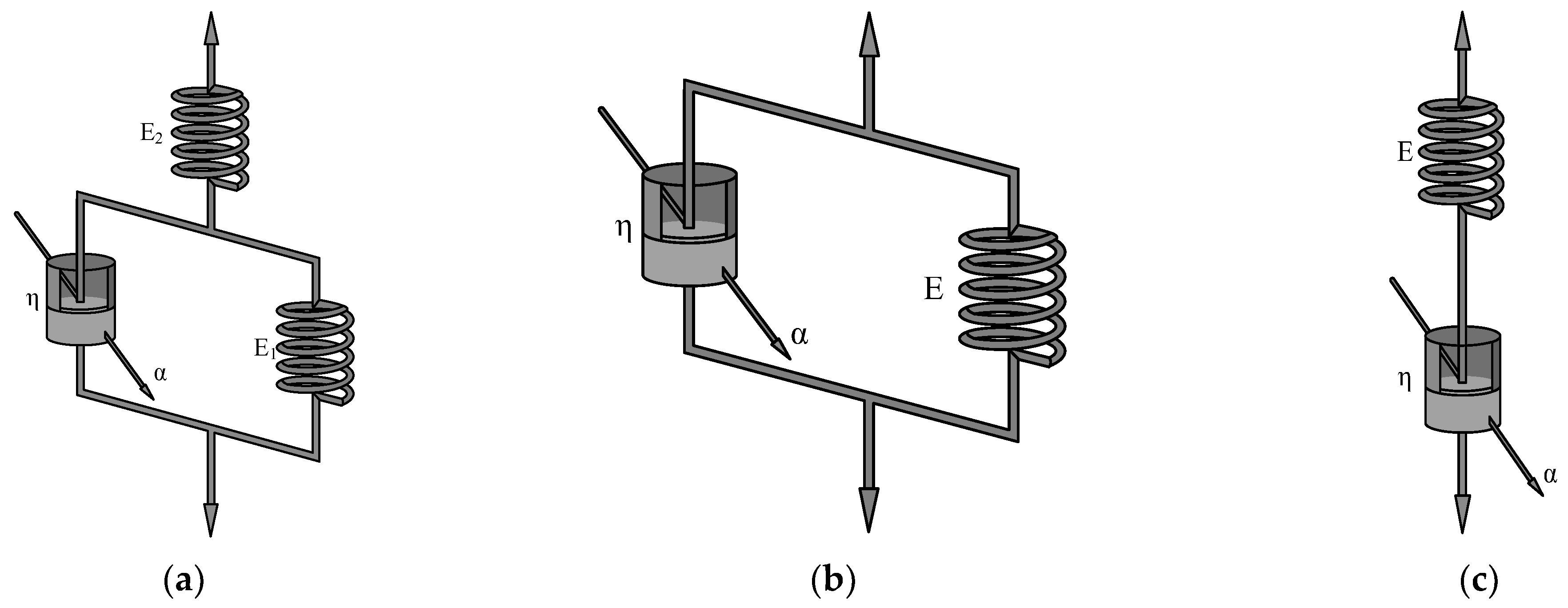
Figure 1. Several fractional derivative viscoelastic models: (a) FTS model; (b) FK model; (c) FM model.
Fractalfract 08 00103 g001
Figure 2. Several classical viscoelastic models: (a) three-parameter model; (b) Kelvin model; (c) Maxwell model.
Fractalfract 08 00103 g002
Figure 3. Finite element calculation model of a cylinder: (a) loads and constraints; (b) meshing; (c) calculation result.
Fractalfract 08 00103 g003
Figure 4. uz of FUMAT and IUMAT at different times: (a) t = 0.01 s; (b) t = 0.1 s; (c) t = 1 s; (d) t = 10 s; (e) t = 100 s; (f) t = 1000 s.
Fractalfract 08 00103 g004
Figure 5. uz of different fractional orders.
Fractalfract 08 00103 g005
Figure 6. uz of several classical viscoelastic models under static load and different temperatures under static load: (a) T = 15 °C; (b) T = 30 °C; (c) T = 45 °C; (d) T = 60 °C.
Fractalfract 08 00103 g006
Figure 7. uz of several fractional derivative viscoelastic models under static load and different temperatures: (a) T = 15 °C; (b) T = 30 °C; (c) T = 45 °C; (d) T = 60 °C.
Fractalfract 08 00103 g007
Figure 8. uz of the three-parameter solid model and FTS under static load and different temperatures: (a) T = 15 °C; (b) T = 30 °C; (c) T = 45 °C; (d) T = 60 °C.
Fractalfract 08 00103 g008aFractalfract 08 00103 g008b
Figure 9. uz of FTS under static load and different temperatures.
Fractalfract 08 00103 g009
Figure 10. uz of FTS under static load and different gradations: (a) T = 15 °C; (b) T = 30 °C; (c) T = 45 °C; (d) T = 60 °C.
Fractalfract 08 00103 g010
Figure 11. uz of FUMAT and IUMAT at time t = T/4: (a) f = 1/32 Hz; (b) f = 1/16 Hz; (c) f = 1/8 Hz; (d) f = 1/4 Hz; (e) f = 1/2 Hz; (f) f = 1 Hz; (g) f = 2 Hz; (h) f = 4 Hz.
Fractalfract 08 00103 g011aFractalfract 08 00103 g011b
Figure 12. uz of FUMAT and IUMAT at time t = T/2: (a) f = 1/32 Hz; (b) f = 1/16 Hz; (c) f = 1/8 Hz; (d) f = 1/4 Hz; (e) f = 1/2 Hz; (f) f = 1 Hz; (g) f = 2 Hz; (h) f = 4 Hz.
Fractalfract 08 00103 g012aFractalfract 08 00103 g012b
Figure 13. uz of several classical viscoelastic models under dynamic load and different temperatures: (a) T = 15 °C; (b) T = 30 °C; (c) T = 45 °C; (d) T = 60 °C.
Fractalfract 08 00103 g013
Figure 14. uz of several fractional derivative viscoelastic models under dynamic load and different temperatures: (a) T = 15 °C; (b) T = 30 °C; (c) T = 45 °C; (d) T = 60 °C.
Fractalfract 08 00103 g014
Figure 15. uz of the three-parameter solid model and FTS under dynamic load and different temperatures: (a) T = 15 °C; (b) T = 30 °C; (c) T = 45 °C; (d) T = 60 °C.
Fractalfract 08 00103 g015aFractalfract 08 00103 g015b
Figure 16. uz of FTS under dynamic load and different temperatures.
Fractalfract 08 00103 g016
Figure 17. uz of FTS under dynamic load and different gradations: (a) T = 15 °C; (b) T = 30 °C; (c) T = 45 °C; (d) T = 60 °C.
Fractalfract 08 00103 g017
Figure 18. Finite element calculation model of a beam: (a) loads and constraints; (b) meshing; (c) calculation result.
Fractalfract 08 00103 g018
Figure 19. ω of FUMAT and IUMAT under different operating conditions: (a) v = 25,000 mm/s, t = 0.01 s; (b) v = 2500 mm/s, t = 0.1 s; (c) v = 250 mm/s, t = 1 s; (d) v = 25 mm/s, t = 10 s.
Fractalfract 08 00103 g019aFractalfract 08 00103 g019b
Figure 20. ω of several classical viscoelastic models under different temperatures: (a) T = 15 °C; (b) T = 30 °C; (c) T = 45 °C; (d) T = 60 °C.
Fractalfract 08 00103 g020
Figure 21. ω of several fractional derivative viscoelastic models under different temperatures: (a) T = 15 °C; (b) T = 30 °C; (c) T = 45 °C; (d) T = 60 °C.
Fractalfract 08 00103 g021
Figure 22. ω of the three-parameter solid model and FTS under different temperatures: (a) T = 15 °C; (b) T = 30 °C; (c) T = 45 °C; (d) T = 60 °C.
Fractalfract 08 00103 g022aFractalfract 08 00103 g022b
Figure 23. ω of FTS under different temperatures.
Fractalfract 08 00103 g023
Figure 24. ω of FTS under different gradations: (a) T = 15 °C; (b) T = 30 °C; (c) T = 45 °C; (d) T = 60 °C.
Fractalfract 08 00103 g024
Table 1. The parameters after the fractional derivative viscoelastic model are degenerated into a linear elasticity model ( α = 0 ).
Parameter TypesFKFMFTS
Elastic modulus E 1 + η E 2 η / E 2 + η E 2 E 1 + η / E 1 + E 2 + η
Poisson’s ratio μ
Table 2. Classical viscoelastic models’ parameters of rubber-modified asphalt mixtures.
Asphalt MixtureTemperature (°C)Fitting Parameters
Kelvin ModelKelvin ModelThree-Parameter Solid Model
EηR2EηR2E1E2ηR2
ARHM-13154929.892.690.464612,602.79957.700.84623115.4314,552.6543.080.9262
301683.621.040.53754604.64299.600.81951031.705526.3313.030.9408
45589.370.320.55321461.25108.330.7521433.681755.654.240.9391
60341.000.160.5339736.4467.920.6305305.63867.062.450.9332
ARHM-20156659.823.210.427015,638.631395.490.82294740.8617,698.8961.160.9119
302345.271.310.50565999.82440.160.81421553.557061.8718.810.9335
451169.860.640.52842906.24218.610.7767835.693451.108.860.9358
60522.610.240.51921123.76105.480.6409466.501314.373.860.9306
ARHM-25158771.204.180.412620,531.811861.680.83196191.5523,092.4583.160.9087
302933.941.700.51247734.54537.870.82391856.929148.6223.510.9369
451634.330.950.53944249.58295.720.79411095.275088.3612.330.9398
60693.000.330.53861557.14134.240.6765586.321843.444.970.9355
Table 3. Fractional derivative viscoelastic models’ parameters of rubber-modified asphalt mixtures.
Asphalt MixtureTemperature (°C)Fitting Parameters
FKFMFTS
EηαR2EηαR2E1E2ηαR2
ARHM-13150.003725.600.16480.99794.83 × 1043893.660.20011.0000123.534.37 × 1043782.630.20811.0000
3078.771113.100.18980.99991.09 × 10261189.090.18340.9997165.583.96 × 1041042.490.21331.0000
45132.81304.550.20001.00005.06 × 1034438.420.16410.9950133.844.15 × 1022303.350.20040.9997
60116.76153.580.19020.99992.57 × 1020279.650.13280.9877115.293.11 × 1029155.460.18860.9999
ARHM-20150.005262.830.14750.99725.12 × 1045754.830.18531.0000109.514.85 × 1045665.140.19011.0000
3053.811686.000.17080.99992.76 × 1061741.710.16800.9998219.344.06 × 1041566.380.19941.0000
45171.29702.530.18451.00001.40 × 1020876.180.16310.9982184.669.78 × 104694.440.18981.0000
60161.27255.520.18091.00001.04 × 1019429.570.13170.9908154.045.09 × 1020263.830.17760.9999
ARHM-25150.006911.070.14730.99545.51 × 1047768.560.19521.000077.095.39 × 1047703.050.19781.0000
3030.182105.140.17570.99982.25 × 1052147.920.17830.9998281.094.36 × 1041909.560.21171.0000
45204.71983.340.19171.00003.76 × 10441189.390.17300.9986248.756.20 × 105952.450.20471.0000
60214.14325.490.19301.00001.51 × 1016553.090.14170.9901215.541.05 × 1034323.850.19350.9999
Table 4. uz of FUMAT and linear elasticity model at time t = T/4 (10−2 mm).
Frequency
(Hz)
α
00.000010.00010.0010.010.1
1/321.415231.415241.415281.415731.420191.46471
1/161.415231.415241.415271.415571.418551.44843
1/81.415231.415241.415251.415401.416921.43207
1/41.415231.415231.415231.415241.415281.41568
1/21.415231.415231.415221.415081.413651.39928
11.415231.415231.415201.414911.412011.38292
21.415241.415231.415191.414751.410381.36664
41.415261.415251.415191.414611.408761.35049
Table 5. uz of FUMAT and linear elastic model at time t = T/2 (10−2 mm).
Frequency
(Hz)
α
01 × 10−101 × 10−91 × 10−81 × 10−71 × 10−61 × 10−51 × 10−4
1/322.1431 × 10−72.1435 × 10−72.1474 × 10−72.1864 × 10−72.5762 × 10−76.4742 × 10−74.5454 × 10−64.3525 × 10−5
1/162.1593 × 10−72.1597 × 10−72.1636 × 10−72.2026 × 10−72.5924 × 10−76.4904 × 10−74.5470 × 10−64.3537 × 10−5
1/82.2019 × 10−72.2023 × 10−72.2062 × 10−72.2452 × 10−72.6350 × 10−76.5329 × 10−74.5513 × 10−64.3531 × 10−5
1/42.1555 × 10−72.1560 × 10−72.1599 × 10−72.1988 × 10−72.5886 × 10−76.4866 × 10−74.5467 × 10−64.3527 × 10−5
1/22.0931 × 10−72.0935 × 10−72.0974 × 10−72.1364 × 10−72.5262 × 10−76.4242 × 10−74.5404 × 10−64.3520 × 10−5
11.8919 × 10−71.8924 × 10−71.8963 × 10−71.9353 × 10−72.3250 × 10−76.2230 × 10−74.5203 × 10−64.3500 × 10−5
29.7809 × 10−79.7852 × 10−79.8242 × 10−81.0214 × 10−71.4112 × 10−75.3092 × 10−74.4289 × 10−64.3409 × 10−5
4−1.7937 × 10⁻⁸−1.7893 × 10⁻⁸−1.7504 × 10⁻⁸−1.3605 × 10−82.5377 × 10−84.1520 × 10−74.3134 × 10−64.3296 × 10⁻⁵
Table 6. ω of FTS and linear elasticity model under different working conditions (mm).
Working Conditionsα
00.000010.00010.0010.010.1
v = 25,000 mm/s, t = 0.01 s0.3173470.3173460.3173330.31720.3158740.302417
v = 2500 mm/s, t = 0.1 s0.3173470.3173470.3173450.3173220.3170920.31466
v = 250 mm/s, t = 1 s0.3173470.3173480.3173570.3174440.318310.326984
v = 25 mm/s, t = 10 s0.3173470.317350.3173690.317570.319530.33905
Disclaimer/Publisher’s Note: The statements, opinions and data contained in all publications are solely those of the individual author(s) and contributor(s) and not of MDPI and/or the editor(s). MDPI and/or the editor(s) disclaim responsibility for any injury to people or property resulting from any ideas, methods, instructions or products referred to in the content.