New Inequalities for GA–h Convex Functions via Generalized Fractional Integral Operators with Applications to Entropy and Mean Inequalities

Abstract

We prove the inequalities of the weighted Hermite–Hadamard type the and Hermite–Hadamard–Mercer type for an extremely rich class of geometrically arithmetically-h-convex functions (GA-h-CFs) via generalized Hadamard–Fractional integral operators (HFIOs). The two generalized fractional integral operators (FIOs) are Hadamard proportional fractional integral operators (HPFIOs) and Hadamard k-fractional integral operators (HKFIOs). Moreover, we also present the results for subclasses of GA-h-CFs and show that the inequalities proved in this paper unify the results from the recent related literature. Furthermore, we compare the two generalizations in view of the fractional operator parameters that contribute to the generalizations of the results and assess the better approximation via graphical tools. Finally, we present applications of the new inequalities via HPFIOs and HKFIOs by establishing interpolation relations between arithmetic mean and geometric mean and by proving the new upper bounds for the Tsallis relative operator entropy.

1. Introduction

Fractional integral and differential operators expand classical calculus by moving from integer orders to fractional ones and have important applications in real-world problems. Fractional operators are highly applicable because they model events with great accuracy. For example, Section 1.3 of [1] highlights their importance in studying materials ranging from liquids to viscoelastic materials. Recently, its applications have expanded to include diverse fields such as science, medicine, and engineering [2,3]. In the class of fractional integral operators (FIOs), the Riemann–Liouville fractional integral operator (RLFIO) is foundational due to its natural generalization [1]. Another operator gaining recent attention in research [4], the Hadamard–Fractional integral operator (HFIO), exhibits isometric properties with the RLFIO [5]. HFIOs have been studied from various perspectives, including mathematical inequalities [6,7], generalized proportional Hadamard fractional integral operators [8], modifications and generalizations like the Caputo [9], and Hadamard k-fractional integrals [10], as well as their relationship with entropy [11].

Mathematical inequalities are one of the most extensively investigated topics in mathematics due to their wide applicability in analyzing key aspects of both classical and modern phenomena. Recently, these inequalities have been utilized to explore system reliability, prediction, and feedback control [12]. The well-known inequalities, including Jensen’s, Hölder’s, Grön-wall’s, and Bihari’s, are crucial for analyzing the controllability of differential equations [13], while Chebyshev’s inequality is used to find certain parameters in data points [14]. Thus, the broad applicability has led to the investigation of mathematical inequalities across diverse domains. Recently, several variants of classical inequalities have been established, including Jensen’s inequality (JI), Jensen–Mercer inequality (JMI), Ostrowski and Fejér-type inequalities [15,16], Hermite–Hadamard inequality (HHI) [17,18], and Young, Heinz and Polya-Szegő-type inequalities [19,20].

Among the numerous mathematical notions involved in investigations of well-known inequalities, the family of convex functions (CFs) [21] stand out as particularly significant. Properties like continuity, differentiability (almost everywhere), and the monotonicity of their derivatives make CFs an important mathematical notion, which has led to their extensive study over time. As a result, various types of CFs, including h-CFs and its subclasses such as s-CFs, P-CFs, Q-CFs, have been introduced and analyzed, with several inequalities developed for these classes. For more details on CFs, generalized CFs, their characteristics, and associated inequalities, see [6,22] and references therein. It is known that the class of h-CFs contains all the above-mentioned classes, thus attaining the most attention in investigations of inequalities [23,24]. In [25], Niculescu introduced the concept of hybrid convexity, referred to as GA-CFs. Similar to how convexity notions have been extended, GA-CFs have also been generalized and modified, leading to different variants of familiar inequalities for GA-CFs and their generalizations [6,7,26,27]. A recent generalization of GA-CFs, referred to as GA-Cr-h-CFs, has been introduced [28] and inequalities known for GA-CFs have been studied for this generalized family of interval-valued functions (IVFs). The recent related studies on Hermite–Hadamard-type, Fejer-type and Mercer-type inequalities for IVFs have also been presented in [16,29]. Several variants of HHI have been proved for different families of functions [30]. For CFs via fractional integrals [31], generalized harmonic CFs on fractal sets [32], the HHI, and related inequalities have been proven. HHI and Jensen-type inequalities have also been investigated in view of the operators, for example, for h-CFs on fractal sets and FIOs [33,34]. Certain inequalities involving variants of CFs, including HH-type inequalities, have been proven for generalized RLFIOs, including multiplicative RLFIOs [35,36]. In recent years, GA-CFs have also received special attention in the context of mathematical inequalities, particular HHI and related ones [6,7,26,28]. However, several inequalities have not yet been investigated for different FIOs and GA-h-CFs and related families, such as [6,28].

In this paper, we prove the inequalities from the [6,7,37,38] by means of two generalized HFIOs, including HPFIO and HKFIO. We prove inequalities involving these operators, which unify the results from [6,7,37,38]. Furthermore, we compare the two generalizations in view of the parameters that contribute to the generalization of the results and assess the approximation via graphical tools. Finally, we present applications of the new inequalities via HPFIOs and HKFIOs by establishing interpolation relations between the arithmetic mean and the geometric mean and by proving the new upper bounds for the Tsallis-relative operator entropy.

2. Basic Notions and Known Results

In this section, we include the necessary definitions and results. For notions not recalled here, we refer [39] to the readers. We use ℜ, 𝚥, $L[x$, $y]$ and h to denote the set of real numbers, an interval in ℜ, a set of integrable functions on $[x,y]$, and a function $h:[0,1]\to [0,\infty )$. We start by recalling the notion of different types of CFs.

Definition 1

([21]). A function $f:𝚥\to \Re$ is called a convex function (CF) if for all $0\le \tau \le 1$ and $x,y\in 𝚥$, the inequality

$$f\left(\tau x+(1-\tau )y\right)\le \tau f\left(x\right)+(1-\tau )f\left(y\right)$$

holds.

Definition 2

([40]). Let function $f:𝚥\to \Re$ and $h:[0,1]\to [0,\infty )$ be two functions; we say that f is h-CF if

$$f\left(\tau x+(1-\tau )y\right)\le h\left(\tau \right)f\left(x\right)+h(1-\tau )f\left(y\right),$$

holds for all $x,y\in 𝚥$ and $0\le \tau \le 1$.

Definition 3

([25]). A function $f:𝚥\subseteq (0,\infty )\to \Re$ is called GA-CF if

$$f\left(x^{\tau }{y}^{1-\tau }\right)\le \tau f\left(x\right)+(1-\tau )f\left(y\right)$$

holds for any $0\le \tau \le 1$ and $x,y\in 𝚥$.

Definition 4

([6]). A function $f:𝚥\subseteq (0,\infty )\to [0,\infty )$ is said to be

•

GA-s-CF if $f\left(x^{\tau }{y}^{1-\tau }\right)\le {\left(\tau \right)}^{s}f\left(x\right)+{(1-\tau )}^{s}f\left(y\right),$

•

GA-Q-CF if $f\left(x^{\tau }{y}^{1-\tau }\right)\le {\displaystyle \frac{f\left(x\right)}{\tau }}+{\displaystyle \frac{f\left(y\right)}{1-\tau }}$,

•

GA-P-CF if $f\left(x^{\tau }{y}^{1-\tau }\right)\le f\left(x\right)+f\left(y\right)$

holds ∀ $\tau \in [0,1]$ ( $\tau \ne 0,1$ for GA-Q-CF), $x,y\in 𝚥$ and $s\in (0,1]$.

Definition 5

([6]). Let $f:𝚥\subseteq (0,\infty )\to [0,\infty )$ and $h:[0,1]\to [0,\infty )$. The function f is known as GA-h-CF if

$$f\left(x^{\tau }{y}^{1-\tau }\right)\le h\left(\tau \right)f\left(x\right)+h(1-\tau )f\left(y\right),$$

holds for any $0\le \tau \le 1$ and $x,y\in 𝚥$.

Remark 1

([6]). If $h\left(\tau \right)=\tau$ (1, ${\tau }^s$ or ${\displaystyle \frac{1}{\tau }}$), the inequality necessary for GA-CFs (GA-P-CF, GA-s-CF or GA-Q-CF) holds. Thus GA-h-CF contains all families, including GA-P-CFs, GA-s-CF, GA-P-CFs, and GA-Q-CFs.

Now, we recall the definition of HFIOs.

Definition 6

([5]). Let $f\in L[x$, $y]$ be a integrable function, with $x<y$ and x, $y\ge 0$. Then,

the left side HHIO of order $\tau >0$ is defined as

$${𝚥}_{y-}^{\tau }f\left(t\right)={\displaystyle \frac{1}{\Gamma \left(\tau \right)}}{\int }_t^y{(ln{\displaystyle \frac{z}{t}})}^{\tau -1}{\displaystyle \frac{f\left(z\right)}{z}}dz.t<y.$$

The right side HFIO of order $\tau >0$ defined as

$${𝚥}_{x+}^{\tau }f\left(t\right)={\displaystyle \frac{1}{\Gamma \left(\tau \right)}}{\int }_x^t{(ln{\displaystyle \frac{t}{z}})}^{\tau -1}{\displaystyle \frac{f\left(z\right)}{z}}dz.x<t.$$

The generalization of HFI known as generalized Hadamard proportional fractional integral operator (GHPFIO) is

Definition 7

([8]). Let $f\in L[x$, $y]$ be a integrable function, with $x<y$ and x, $y\ge 0$ also $p\in (0,1]$; then

The left and right side HPFIO of the order $\tau >0$ are defined by

$${𝚥}_{y-}^{\tau ,p}f\left(t\right)={\displaystyle \frac{1}{p^{\tau }\Gamma \left(\tau \right)}}{\int }_t^y[e^{{\displaystyle \frac{p-1}{p}}ln{\displaystyle \frac{z}{t}}}]{(ln{\displaystyle \frac{z}{t}})}^{\tau -1}{\displaystyle \frac{f\left(z\right)}{z}}dz.t<y$$

and

$${𝚥}_{x+}^{\tau ,p}f\left(t\right)={\displaystyle \frac{1}{p^{\tau }\Gamma \left(\tau \right)}}{\int }_x^t[e^{{\displaystyle \frac{p-1}{p}}ln{\displaystyle \frac{t}{z}}}]{(ln{\displaystyle \frac{t}{z}})}^{\tau -1}{\displaystyle \frac{f\left(z\right)}{z}}dz.x<t$$

Another generalization of HFIO, known as HKFIO, is defined as

Definition 8

([10]). Let $f\in L[x$, $y]$ with $x<y$ and x, $y\ge 0$ and $k>0$.

The left and right side HKFIO of order $\tau >0$ are defined by

$${𝚥}_{y-,k}^{\tau }f\left(t\right)={\displaystyle \frac{1}{k{\Gamma }_k\left(\tau \right)}}{\int }_t^y{(ln{\displaystyle \frac{z}{t}})}^{{\displaystyle \frac{\tau }{k}}-1}{\displaystyle \frac{f\left(z\right)}{z}}dz,t<y$$

and

$${𝚥}_{x+,k}^{\tau }f\left(t\right)={\displaystyle \frac{1}{k{\Gamma }_k\left(\tau \right)}}{\int }_x^t{(ln{\displaystyle \frac{t}{z}})}^{{\displaystyle \frac{\tau }{k}}-1}{\displaystyle \frac{f\left(z\right)}{z}}dz,x<t,$$

where

$${\Gamma }_k\left(\tau \right):={\int }_0^{\infty }{t}^{\tau -1}exp\left(-{\displaystyle \frac{t^k}{k}}\right)dt,\mathrm{Re}\left(\tau \right)>0.$$

Note that, if $p=k=1$ in HPFIO and HKFIO, then we obtain HFIO.

Now, we recall the main results involving HFIs from [6]. Throughout this manuscript, we assume that $\mu >0.$

Theorem 1.

For a GA-h-CF f on $[\mu ,\nu ]$ and an integrable function ϕ on $[\mu ,\nu ]$, the inequalities

$$\begin{array}{c}{\displaystyle \frac{1}{2h\left(\frac{1}{2}\right)}}f\left({\displaystyle \frac{\mu \nu }{\sqrt{xy}}}\right){\int }_{{\displaystyle \frac{\mu \nu }{y}}}^{{\displaystyle \frac{\mu \nu }{x}}}{\displaystyle \frac{\varphi \left(z\right)}{z}}dz\le {\displaystyle \frac{1}{2}}\left[{\int }_{{\displaystyle \frac{\mu \nu }{y}}}^{{\displaystyle \frac{\mu \nu }{x}}}f\left(z\right)\varphi \left(z\right){\displaystyle \frac{dz}{z}}+{\int }_{{\displaystyle \frac{\mu \nu }{y}}}^{{\displaystyle \frac{\mu \nu }{x}}}f\left(z\right)\varphi \left({\displaystyle \frac{{\left(\mu \nu \right)}^2}{xyz}}\right){\displaystyle \frac{dz}{z}}\right]\hfill \\ \le {\displaystyle \frac{1}{2}}\left[f\left({\displaystyle \frac{\mu \nu }{x}}\right)+f\left({\displaystyle \frac{\mu \nu }{y}}\right)\right]{\int }_{{\displaystyle \frac{\mu \nu }{y}}}^{{\displaystyle \frac{\mu \nu }{x}}}\left[h\left({\displaystyle \frac{ln\left(\frac{yz}{\mu \nu }\right)}{ln\left(\frac{y}{x}\right)}}\right)+h\left({\displaystyle \frac{ln\left(\frac{\mu \nu }{xz}\right)}{ln\left(\frac{y}{x}\right)}}\right)\right]\varphi \left(z\right){\displaystyle \frac{dz}{z}}\\ \le \left[f\left(\mu \right)+f\left(\nu \right)\right]{\int }_{{\displaystyle \frac{\mu \nu }{y}}}^{{\displaystyle \frac{\mu \nu }{x}}}{\left[h\left({\displaystyle \frac{ln\left(\frac{yz}{\mu \nu }\right)}{ln\left(\frac{y}{x}\right)}}\right)+h\left({\displaystyle \frac{ln\left(\frac{\mu \nu }{xz}\right)}{ln\left(\frac{y}{x}\right)}}\right)\right]}^2\varphi \left(z\right){\displaystyle \frac{dz}{z}}\\ \hfill -\left[{\displaystyle \frac{f\left(x\right)+f\left(y\right)}{2}}\right]{\int }_{{\displaystyle \frac{\mu \nu }{y}}}^{{\displaystyle \frac{\mu \nu }{x}}}\left[h\left({\displaystyle \frac{ln\left(\frac{yz}{\mu \nu }\right)}{ln\left(\frac{y}{x}\right)}}\right)+h\left({\displaystyle \frac{ln\left(\frac{\mu \nu }{xz}\right)}{ln\left(\frac{y}{x}\right)}}\right)\right]\varphi \left(z\right){\displaystyle \frac{dz}{z}},\end{array}$$

(1)

hold for all $x,y\in [\mu ,\nu ]$, where $h\left({\displaystyle \frac{1}{2}}\right)\ne 0$.

Theorem 2.

For a GA-h-CF f on $[\mu ,\nu ]$ and an integrable function ϕ on $[\mu ,\nu ]$, the inequalities

$$\begin{array}{c}{\displaystyle \frac{1}{2h\left(\frac{1}{2}\right)}}f\left({\displaystyle \frac{\mu \nu }{\sqrt{xy}}}\right){\int }_{{\displaystyle \frac{\mu \nu }{y}}}^{{\displaystyle \frac{\mu \nu }{x}}}{\displaystyle \frac{\varphi \left(z\right)}{z}}dz\le {\displaystyle \frac{1}{2}}\left[{\int }_{{\displaystyle \frac{\mu \nu }{y}}}^{{\displaystyle \frac{\mu \nu }{x}}}f\left(z\right)\varphi \left(z\right){\displaystyle \frac{dz}{z}}+{\int }_{{\displaystyle \frac{\mu \nu }{y}}}^{{\displaystyle \frac{\mu \nu }{x}}}f\left(z\right)\varphi \left({\displaystyle \frac{{\left(\mu \nu \right)}^2}{xyz}}\right){\displaystyle \frac{dz}{z}}\right]\hfill \\ \le [f\left(\mu \right)+f\left(\nu \right)]{\int }_x^y\left[h\left({\displaystyle \frac{ln\left(\frac{z}{y}\right)}{ln\left(\frac{x}{y}\right)}}\right)+h\left({\displaystyle \frac{ln\left(\frac{x}{z}\right)}{ln\left(\frac{x}{y}\right)}}\right)\right]\varphi \left({\displaystyle \frac{\mu \nu }{z}}\right){\displaystyle \frac{dz}{z}}-\\ {\displaystyle \frac{1}{2}}\left[{\int }_x^{y}f\left(z\right)\varphi \left({\displaystyle \frac{\mu \nu }{z}}\right){\displaystyle \frac{dz}{z}}+{\int }_x^{y}f\left(z\right)\varphi \left({\displaystyle \frac{\mu \nu z}{xv}}\right){\displaystyle \frac{dz}{z}}\right]\\ \hfill \le [f\left(\mu \right)+f\left(\nu \right)]{\int }_x^y\left[h\left({\displaystyle \frac{ln\left(\frac{z}{y}\right)}{ln\left(\frac{x}{y}\right)}}\right)+h\left({\displaystyle \frac{ln\left(\frac{x}{z}\right)}{ln\left(\frac{x}{y}\right)}}\right)\right]\varphi \left({\displaystyle \frac{\mu \nu }{z}}\right){\displaystyle \frac{dz}{z}}-{\displaystyle \frac{1}{2h\left(\frac{1}{2}\right)}}f\left(\sqrt{xy}\right){\int }_x^y\varphi \left({\displaystyle \frac{\mu \nu }{z}}\right){\displaystyle \frac{dz}{z}},\end{array}$$

(2)

hold for all $x,y\in [\mu ,\nu ]$ and $h\left({\displaystyle \frac{1}{2}}\right)\ne 0$.

3. Results

In this section, we prove Hermite–Hadamard–Mercer and weighted Hermite– Hadamard-type inequalities for GA-h-CFs in terms of HPFIOs. We extract several consequences from the main results. Moreover, the inequalities involving HPFIOs for special cases GA-CFs, GA-s-CFs, GA-P-CFs and GA-$QP$-CFs have also been obtained. In the end, by using the special cases for the HPFIO, we re-capture the main results of several recent contributions in the area of mathematical inequalities.

In order to prove the main results, we introduce the following: For any $x,y\in [\mu ,\nu ]$ with $\mu >0$ and $x<y$, the functions $f,\varphi \in L[\mu ,\nu ]$ and a function $h:[0,1]\to [0,\infty )$, we define

$$\begin{array}{c}{H}_{\mu ,x}^{\nu ,y}(f,\varphi ,h)={\displaystyle \frac{1}{2}}\left[{\int }_{{\displaystyle \frac{\mu \nu }{y}}}^{{\displaystyle \frac{\mu \nu }{x}}}f\left(z\right)\varphi \left(z\right){\displaystyle \frac{dz}{z}}+{\int }_{{\displaystyle \frac{\mu \nu }{y}}}^{{\displaystyle \frac{\mu \nu }{x}}}f\left(z\right)\varphi \left({\displaystyle \frac{{\left(\mu \nu \right)}^2}{xyz}}\right){\displaystyle \frac{dz}{z}}\right]-\hfill \\ \hfill {\displaystyle \frac{1}{2h\left(\frac{1}{2}\right)}}f\left({\displaystyle \frac{\mu \nu }{\sqrt{xy}}}\right){\int }_{{\displaystyle \frac{\mu \nu }{y}}}^{{\displaystyle \frac{\mu \nu }{x}}}{\displaystyle \frac{\varphi \left(z\right)}{z}}dz.\end{array}$$

(3)

Under the assumption that if f is GA-h-CF f on $[\mu ,\nu ]$, then Theorem 1 implies that $H_{\mu ,x}^{\nu ,y}(f,\varphi ,h)\ge 0$.

Now, we are ready to prove the following main result.

Theorem 3.

For a GA-h-CF f on $[\mu ,\nu ]$, $p\in (0,1]$ and $\tau >0$, the inequalities

$$\begin{array}{c}\hfill {\displaystyle \frac{1}{2h\left(\frac{1}{2}\right)}}f\left({\displaystyle \frac{\mu \nu }{\sqrt{xy}}}\right)\left\{{\displaystyle \frac{{ln}^{\tau }\left(\frac{y}{x}\right)e^{\frac{p-1}{p}ln\left(\frac{y}{x}\right)}-\frac{p-1}{p}{\int }_{\frac{\mu \nu }{y}}^{\frac{\mu \nu }{x}}{ln}^{\tau }\left(\frac{\mu \nu }{zx}\right)e^{\frac{p-1}{p}ln\left(\frac{\mu \nu }{zx}\right)}\frac{dz}{z}}{p^{\tau }\Gamma (\tau +1)}}\right\}\\ \hfill \le {\displaystyle \frac{1}{2}}\left\{{𝚥}_{{\displaystyle \frac{\mu \nu }{y}}+}^{\tau ,p}f\left({\displaystyle \frac{\mu \nu }{x}}\right)+{𝚥}_{{\displaystyle \frac{\mu \nu }{x}}-}^{\tau ,p}f\left({\displaystyle \frac{\mu \nu }{y}}\right)\right\}\\ \hfill \le {\displaystyle \frac{1}{2}}\left[f\left({\displaystyle \frac{\mu \nu }{x}}\right)+f\left({\displaystyle \frac{\mu \nu }{y}}\right)\right]{\int }_{{\displaystyle \frac{\mu \nu }{y}}}^{{\displaystyle \frac{\mu \nu }{x}}}\left[h\left({\displaystyle \frac{ln\left(\frac{yz}{\mu \nu }\right)}{ln\left(\frac{y}{x}\right)}}\right)+h\left({\displaystyle \frac{ln\left(\frac{\mu \nu }{xz}\right)}{ln\left(\frac{y}{x}\right)}}\right)\right]e^{{\displaystyle \frac{p-1}{p}}ln\left({\displaystyle \frac{\mu \nu }{zx}}\right)}{\displaystyle \frac{{ln}^{\tau -1}\left(\frac{\mu \nu }{xz}\right)}{p^{\tau }\Gamma \left(\tau \right)z}}dz\end{array}$$

$$\begin{array}{c}\hfill \le [f\left(\mu \right)+f\left(\nu \right)]{\int }_{{\displaystyle \frac{\mu \nu }{y}}}^{{\displaystyle \frac{\mu \nu }{x}}}{\left[h\left({\displaystyle \frac{ln\left(\frac{yz}{\mu \nu }\right)}{ln\left(\frac{y}{x}\right)}}\right)+h\left({\displaystyle \frac{ln\left(\frac{\mu \nu }{xz}\right)}{ln\left(\frac{y}{x}\right)}}\right)\right]}^2{e}^{{\displaystyle \frac{p-1}{p}}ln\left({\displaystyle \frac{\mu \nu }{zx}}\right)}{\displaystyle \frac{{ln}^{\tau -1}\left(\frac{\mu \nu }{xz}\right)}{p^{\tau }\Gamma \left(\tau \right)z}}dz\\ \hfill -{\displaystyle \frac{1}{2}}[f\left(x\right)+f\left(y\right)]{\int }_{{\displaystyle \frac{\mu \nu }{y}}}^{{\displaystyle \frac{\mu \nu }{x}}}\left[h\left({\displaystyle \frac{ln\left(\frac{yz}{\mu \nu }\right)}{ln\left(\frac{y}{x}\right)}}\right)+h\left({\displaystyle \frac{ln\left(\frac{\mu \nu }{xz}\right)}{ln\left(\frac{y}{x}\right)}}\right)\right]e^{{\displaystyle \frac{p-1}{p}}ln\left({\displaystyle \frac{\mu \nu }{zx}}\right)}{\displaystyle \frac{{ln}^{\tau -1}\left(\frac{\mu \nu }{xz}\right)}{p^{\tau }\Gamma \left(\tau \right)z}}dz\end{array}$$

hold for all $x,y\in [\mu ,\nu ]$, where $h\left({\displaystyle \frac{1}{2}}\right)\ne 0$.

Proof. 

To prove the first inequality, we substitute $\varphi \left(z\right)={\displaystyle \frac{1}{p^{\tau }\Gamma \left(\tau \right)}}{e}^{{\displaystyle \frac{p-1}{p}}ln\left({\displaystyle \frac{\mu \nu }{zx}}\right)}{ln}^{\tau -1}\left({\displaystyle \frac{\mu \nu }{zx}}\right)$ in Equation (3); we have

$$\begin{array}{c}{H}_{\mu ,x}^{\nu ,y}\left(f,{\displaystyle \frac{1}{p^{\tau }\Gamma \left(\tau \right)}}{e}^{{\displaystyle \frac{p-1}{p}}ln\left({\displaystyle \frac{\mu \nu }{zx}}\right)}{ln}^{\tau -1}\left({\displaystyle \frac{\mu \nu }{zx}}\right),h\right)=\hfill \\ {\displaystyle \frac{1}{2}}\left[{\int }_{{\displaystyle \frac{\mu \nu }{y}}}^{{\displaystyle \frac{\mu \nu }{x}}}f\left(z\right){\displaystyle \frac{1}{p^{\tau }\Gamma \left(\tau \right)}}{e}^{{\displaystyle \frac{p-1}{p}}ln\left({\displaystyle \frac{\mu \nu }{zx}}\right)}{ln}^{\tau -1}\left({\displaystyle \frac{\mu \nu }{zx}}\right){\displaystyle \frac{dz}{z}}+{\int }_{{\displaystyle \frac{\mu \nu }{y}}}^{{\displaystyle \frac{\mu \nu }{x}}}f\left(z\right){\displaystyle \frac{1}{p^{\tau }\Gamma \left(\tau \right)}}{e}^{{\displaystyle \frac{p-1}{p}}ln\left({\displaystyle \frac{yz}{\mu \nu }}\right)}{ln}^{\tau -1}\left({\displaystyle \frac{yz}{\mu \nu }}\right){\displaystyle \frac{dz}{z}}\right]\\ \hfill -{\displaystyle \frac{1}{2h\left(\frac{1}{2}\right)}}f\left({\displaystyle \frac{\mu \nu }{\sqrt{xy}}}\right){\int }_{{\displaystyle \frac{\mu \nu }{y}}}^{{\displaystyle \frac{\mu \nu }{x}}}{\displaystyle \frac{1}{p^{\tau }\Gamma \left(\tau \right)}}{e}^{{\displaystyle \frac{p-1}{p}}ln\left({\displaystyle \frac{\mu \nu }{zx}}\right)}{ln}^{\tau -1}\left({\displaystyle \frac{\mu \nu }{zx}}\right){\displaystyle \frac{dz}{z}}.\end{array}$$

$$\begin{array}{c}\hfill ={\displaystyle \frac{1}{2}}\left[{\displaystyle \frac{1}{p^{\tau }\Gamma \left(\tau \right)}}{\int }_{{\displaystyle \frac{\mu \nu }{y}}}^{{\displaystyle \frac{\mu \nu }{x}}}{e}^{{\displaystyle \frac{p-1}{p}}ln\left({\displaystyle \frac{\mu \nu }{zx}}\right)}{ln}^{\tau -1}\left({\displaystyle \frac{\mu \nu }{zx}}\right)f\left(z\right){\displaystyle \frac{dz}{z}}+{\displaystyle \frac{1}{p^{\tau }\Gamma \left(\tau \right)}}{\int }_{{\displaystyle \frac{\mu \nu }{y}}}^{{\displaystyle \frac{\mu \nu }{x}}}{e}^{{\displaystyle \frac{p-1}{p}}ln\left({\displaystyle \frac{yz}{\mu \nu }}\right)}{ln}^{\tau -1}\left({\displaystyle \frac{yz}{\mu \nu }}\right)f\left(z\right){\displaystyle \frac{dz}{z}}\right]\\ \hfill -{\displaystyle \frac{1}{2h\left(\frac{1}{2}\right)}}f\left({\displaystyle \frac{\mu \nu }{\sqrt{xy}}}\right){\displaystyle \frac{1}{p^{\tau }\Gamma \left(\tau \right)}}{\int }_{{\displaystyle \frac{\mu \nu }{y}}}^{{\displaystyle \frac{\mu \nu }{x}}}{ln}^{\tau -1}\left({\displaystyle \frac{\mu \nu }{zx}}\right)e^{{\displaystyle \frac{p-1}{p}}ln\left({\displaystyle \frac{\mu \nu }{zx}}\right)}{\displaystyle \frac{dz}{z}}.\end{array}$$

$$\begin{array}{c}{H}_{\mu ,x}^{\nu ,y}\left(f,{\displaystyle \frac{1}{p^{\tau }\Gamma \left(\tau \right)}}{e}^{{\displaystyle \frac{p-1}{p}}ln\left({\displaystyle \frac{\mu \nu }{zx}}\right)}{ln}^{\tau -1}\left({\displaystyle \frac{\mu \nu }{zx}}\right),h\right)={\displaystyle \frac{1}{2}}\left\{{𝚥}_{{\displaystyle \frac{\mu \nu }{y}}+}^{\tau ,p}f\left({\displaystyle \frac{\mu \nu }{x}}\right)+{𝚥}_{{\displaystyle \frac{\mu \nu }{x}}-}^{\tau ,p}f\left({\displaystyle \frac{\mu \nu }{y}}\right)\right\}\hfill \\ \hfill -{\displaystyle \frac{1}{2h\left(\frac{1}{2}\right)}}f\left({\displaystyle \frac{\mu \nu }{\sqrt{xy}}}\right)\left[{\displaystyle \frac{{ln}^{\tau }\left(\frac{y}{x}\right)e^{\frac{p-1}{p}ln\left(\frac{y}{x}\right)}-\frac{p-1}{p}{\int }_{\frac{\mu \nu }{y}}^{\frac{\mu \nu }{x}}{ln}^{\tau }\left(\frac{\mu \nu }{zx}\right)e^{\frac{p-1}{p}ln\left(\frac{\mu \nu }{zx}\right)}\frac{dz}{z}}{p^{\tau }\Gamma (\tau +1)}}\right].\end{array}$$

Since f is GA-h-CF, $H_{\mu ,u}^{\nu ,v}(f,{\displaystyle \frac{1}{p^{\tau }\Gamma \left(\tau \right)}}{e}^{{\displaystyle \frac{p-1}{p}}ln\left({\displaystyle \frac{\mu \nu }{zu}}\right)}{ln}^{\tau -1}\left({\displaystyle \frac{\mu \nu }{zx}}\right),h)\ge$ 0. So

$$\begin{array}{c}\hfill 0\le {\displaystyle \frac{1}{2}}\left\{{𝚥}_{{\displaystyle \frac{\mu \nu }{y}}+}^{\tau ,p}f\left({\displaystyle \frac{\mu \nu }{x}}\right)+{𝚥}_{{\displaystyle \frac{\mu \nu }{x}}-}^{\tau ,p}f\left({\displaystyle \frac{\mu \nu }{y}}\right)\right\}-\\ \hfill \left[{\displaystyle \frac{1}{2h\left(\frac{1}{2}\right)}}f\left({\displaystyle \frac{\mu \nu }{\sqrt{xy}}}\right)\left\{{\displaystyle \frac{{ln}^{\tau }\left(\frac{y}{x}\right)e^{\frac{p-1}{p}ln\left(\frac{y}{x}\right)}-\frac{p-1}{p}{\int }_{\frac{\mu \nu }{y}}^{\frac{\mu \nu }{x}}{ln}^{\tau }\left(\frac{\mu \nu }{zx}\right)e^{\frac{p-1}{p}ln\left(\frac{\mu \nu }{zx}\right)}\frac{dz}{z}}{p^{\tau }\Gamma (\tau +1)}}\right\}\right]\end{array}$$

The above inequality produces the following inequality:

$$\begin{array}{c}\hfill {\displaystyle \frac{1}{2h\left(\frac{1}{2}\right)}}f\left({\displaystyle \frac{\mu \nu }{\sqrt{xy}}}\right)\left\{{\displaystyle \frac{{ln}^{\tau }\left(\frac{y}{x}\right)e^{\frac{p-1}{p}ln\left(\frac{y}{x}\right)}-\frac{p-1}{p}{\int }_{\frac{\mu \nu }{y}}^{\frac{\mu \nu }{x}}{ln}^{\tau }\left(\frac{\mu \nu }{zx}\right)e^{\frac{p-1}{p}ln\left(\frac{\mu \nu }{zx}\right)}\frac{dz}{z}}{p^{\tau }\Gamma (\tau +1)}}\right\}\\ \hfill \le {\displaystyle \frac{1}{2}}\left\{{𝚥}_{{\displaystyle \frac{\mu \nu }{y}}+}^{\tau ,p}f\left({\displaystyle \frac{\mu \nu }{x}}\right)+{𝚥}_{{\displaystyle \frac{\mu \nu }{x}}-}^{\tau ,p}f\left({\displaystyle \frac{\mu \nu }{y}}\right)\right\}\end{array}$$

for all $x,y\in [\mu ,\nu ]$ and $h\left({\displaystyle \frac{1}{2}}\right)\ne 0$. Thus, we obtain the first inequality. The other inequalities directly follow by substituting $\varphi \left(z\right)={\displaystyle \frac{1}{p^{\tau }\Gamma \left(\tau \right)}}{e}^{{\displaystyle \frac{p-1}{p}}ln\left({\displaystyle \frac{\mu \nu }{zx}}\right)}{ln}^{\tau -1}\left({\displaystyle \frac{\mu \nu }{zx}}\right)$ in Theorem 1, which completes the proof. □

By replacing $h\left(\lambda \right)=\lambda$ in Theorem 3, we obtain the following results:

Corollary 1.

for a GA-CF f on $[\mu ,\nu ]$, $p\in (0,1]$ and $\tau >0$, the inequalities

$$\begin{array}{c}\hfill f\left({\displaystyle \frac{\mu \nu }{\sqrt{xy}}}\right)\le \left[{\displaystyle \frac{p^{\tau }\Gamma (\tau +1)}{2\left[{ln}^{\tau }\left(\frac{y}{x}\right)e^{\frac{p-1}{p}ln\left(\frac{y}{x}\right)}-\frac{p-1}{p}{\int }_{\frac{\mu \nu }{y}}^{\frac{\mu \nu }{x}}{ln}^{\tau }\left(\frac{\mu \nu }{zx}\right)e^{\frac{p-1}{p}ln\left(\frac{\mu \nu }{zx}\right)}\frac{dz}{z}\right]}}\right]\left\{{𝚥}_{{\displaystyle \frac{\mu \nu }{y}}+}^{\tau ,p}f\left({\displaystyle \frac{\mu \nu }{x}}\right)+{𝚥}_{{\displaystyle \frac{\mu \nu }{x}}-}^{\tau ,p}f\left({\displaystyle \frac{\mu \nu }{y}}\right)\right\}\\ \hfill \le {\displaystyle \frac{1}{2}}\left[f\left({\displaystyle \frac{\mu \nu }{x}}\right)+f\left({\displaystyle \frac{\mu \nu }{y}}\right)\right]\le [f\left(\mu \right)+f\left(\nu \right)]-{\displaystyle \frac{f\left(x\right)+f\left(y\right)}{2}}\end{array}$$

for all $x,y\in [\mu ,\nu ]$.

By replacing $x=\mu$ and $y=\nu$ in Theorem 3, we obtain the following results:

Corollary 2.

For a GA-h-CF f on $[\mu ,\nu ]$, $p\in (0,1]$ and $\tau >0$, the inequalities

$$\begin{array}{c}\hfill {\displaystyle \frac{1}{2h\left(\frac{1}{2}\right)}}f\left(\sqrt{\mu \nu }\right)\left\{{\displaystyle \frac{{ln}^{\tau }\left(\frac{\nu }{\mu }\right)e^{\frac{p-1}{p}ln\left(\frac{\nu }{\mu }\right)}-\frac{p-1}{p}{\int }_{\mu }^{\nu }{ln}^{\tau }\left(\frac{\nu }{z}\right)e^{\frac{p-1}{p}ln\left(\frac{\nu }{z}\right)}\frac{dz}{z}}{p^{\tau }\Gamma (\tau +1)}}\right\}\le {\displaystyle \frac{1}{2}}\left\{{𝚥}_{\mu +}^{\tau ,p}f\left(\nu \right)+{𝚥}_{\nu -}^{\tau ,p}f\left(\mu \right)\right\}\\ \hfill \le {\displaystyle \frac{1}{2}}\left[f\left(\nu \right)+f\left(\mu \right)\right]{\int }_{\mu }^{\nu }\left[h\left({\displaystyle \frac{ln\left(\frac{z}{\mu }\right)}{ln\left(\frac{\nu }{\mu }\right)}}\right)+h\left({\displaystyle \frac{ln\left(\frac{\nu }{z}\right)}{ln\left(\frac{\nu }{\mu }\right)}}\right)\right]e^{{\displaystyle \frac{p-1}{p}}ln\left({\displaystyle \frac{\nu }{z}}\right)}{\displaystyle \frac{{ln}^{\tau -1}\left(\frac{\nu }{z}\right)}{p^{\tau }\Gamma \left(\tau \right)z}}dz\\ \hfill \le [f\left(\mu \right)+f\left(\nu \right)]{\int }_{\mu }^{\nu }{\left[h\left({\displaystyle \frac{ln\left(\frac{z}{\mu }\right)}{ln\left(\frac{\nu }{\mu }\right)}}\right)+h\left({\displaystyle \frac{ln\left(\frac{\nu }{z}\right)}{ln\left(\frac{\nu }{\mu }\right)}}\right)\right]}^2{e}^{{\displaystyle \frac{p-1}{p}}ln\left({\displaystyle \frac{\nu }{z}}\right)}{\displaystyle \frac{{ln}^{\tau -1}\left(\frac{\nu }{z}\right)}{p^{\tau }\Gamma \left(\tau \right)z}}dz\\ \hfill -{\displaystyle \frac{1}{2}}[f\left(\mu \right)+f\left(\nu \right)]{\int }_{\mu }^{\nu }\left[h\left({\displaystyle \frac{ln\left(\frac{z}{\mu }\right)}{ln\left(\frac{\nu }{\mu }\right)}}\right)+h\left({\displaystyle \frac{ln\left(\frac{\nu }{z}\right)}{ln\left(\frac{\nu }{\mu }\right)}}\right)\right]e^{{\displaystyle \frac{p-1}{p}}ln\left({\displaystyle \frac{\nu }{z}}\right)}{\displaystyle \frac{{ln}^{\tau -1}\left(\frac{\nu }{z}\right)}{p^{\tau }\Gamma \left(\tau \right)z}}dz,\end{array}$$

hold, where $h\left({\displaystyle \frac{1}{2}}\right)\ne 0.$

By replacing $h\left(\lambda \right)=\lambda$ in Corollary 2, we obtain the following results

Corollary 3.

For a GA-CF f on $[\mu ,\nu ]$, $p\in (0,1]$ and $\tau >0$, the inequalities

$$\begin{array}{cc}\hfill & f\left(\sqrt{\mu \nu }\right)\left\{{\displaystyle \frac{{ln}^{\tau }\left(\frac{\nu }{\mu }\right)e^{\frac{p-1}{p}ln\left(\frac{\nu }{\mu }\right)}-\frac{p-1}{p}{\int }_{\mu }^{\nu }{ln}^{\tau }\left(\frac{\nu }{z}\right)e^{\frac{p-1}{p}ln\left(\frac{\nu }{z}\right)}\frac{dz}{z}}{p^{\tau }\Gamma (\tau +1)}}\right\}\hfill \\ \hfill & \le {\displaystyle \frac{1}{2}}\left\{{𝚥}_{\mu +}^{\tau ,p}f\left(\nu \right)+{𝚥}_{\nu -}^{\tau ,p}f\left(\mu \right)\right\}\hfill \\ \hfill & \le {\displaystyle \frac{f\left(\nu \right)+f\left(\mu \right)}{2}}\left\{{\displaystyle \frac{{ln}^{\tau }\left(\frac{\nu }{\mu }\right)e^{\frac{p-1}{p}ln\left(\frac{\nu }{\mu }\right)}-\frac{p-1}{p}{\int }_{\mu }^{\nu }{ln}^{\tau }\left(\frac{\nu }{z}\right)e^{\frac{p-1}{p}ln\left(\frac{\nu }{z}\right)}\frac{dz}{z}}{p^{\tau }\Gamma (\tau +1)}}\right\}\hfill \end{array}$$

hold.

If we put $\varphi \left(z\right)={\displaystyle \frac{1}{p^{\tau }\Gamma \left(\tau \right)}}{e}^{{\displaystyle \frac{p-1}{p}}ln\left({\displaystyle \frac{\mu \nu }{zx}}\right)}{ln}^{\tau -1}\left({\displaystyle \frac{\mu \nu }{zx}}\right)$ or $\varphi \left(z\right)={\displaystyle \frac{1}{p^{\tau }\Gamma \left(\tau \right)}}{e}^{{\displaystyle \frac{p-1}{p}}ln\left({\displaystyle \frac{yz}{\mu \nu }}\right)}{ln}^{\tau -1}\left({\displaystyle \frac{yz}{\mu \nu }}\right)$ in Theorem 2, we obtain the following inequalities.

Theorem 4.

For a GA-h-CF f on $[\mu ,\nu ]$, $p\in (0,1]$ and $\tau >0$, the inequalities

$$\begin{array}{c}{\displaystyle \frac{1}{2h\left(\frac{1}{2}\right)}}f\left({\displaystyle \frac{\mu \nu }{\sqrt{xy}}}\right)\left\{{\displaystyle \frac{{ln}^{\tau }\left(\frac{y}{x}\right)e^{\frac{p-1}{p}ln\left(\frac{y}{x}\right)}-\frac{p-1}{p}{\int }_{\frac{\mu \nu }{y}}^{\frac{\mu \nu }{x}}{ln}^{\tau }\left(\frac{\mu \nu }{zx}\right)e^{\frac{p-1}{p}ln\left(\frac{\mu \nu }{zx}\right)}\frac{dz}{z}}{p^{\tau }\Gamma (\tau +1)}}\right\}\hfill \\ \le {\displaystyle \frac{1}{2}}\{{𝚥}_{{\displaystyle \frac{\mu \nu }{y}}+}^{\tau ,p}f\left({\displaystyle \frac{\mu \nu }{x}}\right)+{𝚥}_{{\displaystyle \frac{\mu \nu }{x}}-}^{\tau ,p}f\left({\displaystyle \frac{\mu \nu }{y}}\right)\}\\ \le [f\left(\mu \right)+f\left(\nu \right)]{\int }_x^y\left[h\left({\displaystyle \frac{ln\left(\frac{z}{y}\right)}{ln\left(\frac{x}{y}\right)}}\right)+h\left({\displaystyle \frac{ln\left(\frac{x}{z}\right)}{ln\left(\frac{x}{y}\right)}}\right)\right]{\displaystyle \frac{e^{\frac{p-1}{p}ln\left(\frac{z}{x}\right)}{ln}^{\tau -1}\left(\frac{z}{x}\right)}{z{p}^{\tau }\Gamma \left(\tau \right)}}dz-{\displaystyle \frac{1}{2}}\left[{𝚥}_{y-}^{\tau ,p}f\left(u\right)+{𝚥}_{x+}^{\tau ,p}f\left(y\right)\right]\\ \le [f\left(\mu \right)+f\left(\nu \right)]{\int }_x^y\left[h\left({\displaystyle \frac{ln\left(\frac{z}{y}\right)}{ln\left(\frac{x}{y}\right)}}\right)+h\left({\displaystyle \frac{ln\left(\frac{x}{z}\right)}{ln\left(\frac{x}{y}\right)}}\right)\right]{\displaystyle \frac{e^{\frac{p-1}{p}ln\left(\frac{z}{x}\right)}{ln}^{\tau -1}\left(\frac{z}{x}\right)}{z{p}^{\tau }\Gamma \left(\tau \right)}}dz\\ \hfill -{\displaystyle \frac{1}{2h\left(\frac{1}{2}\right)}}f\left(\sqrt{xy}\right)\left\{{\displaystyle \frac{{ln}^{\tau }\left(\frac{y}{x}\right)e^{\frac{p-1}{p}ln\left(\frac{y}{x}\right)}-\frac{p-1}{p}{\int }_{\frac{\mu \nu }{y}}^{\frac{\mu \nu }{x}}{ln}^{\tau }\left(\frac{\mu \nu }{zx}\right)e^{\frac{p-1}{p}ln\left(\frac{\mu \nu }{zx}\right)}\frac{dz}{z}}{p^{\tau }\Gamma (\tau +1)}}\right\},\end{array}$$

(4)

hold for all $x,y\in [\mu ,\nu ]$, where $h\left({\displaystyle \frac{1}{2}}\right)\ne 0$.

By replacing $h\left(\lambda \right)=\lambda$ in Theorem 4, we obtain the following result for GA-CFs through GHPFI.

Corollary 4.

For a GA-CF f on $[\mu ,\nu ]$, $p\in (0,1]$ and $\tau >0$, the inequalities

$$\begin{array}{c}f\left({\displaystyle \frac{\mu \nu }{\sqrt{xy}}}\right)\le {\displaystyle \frac{1}{2}}\left\{{\displaystyle \frac{p^{\tau }\Gamma (\tau +1)}{{ln}^{\tau }\left(\frac{y}{x}\right)e^{\frac{p-1}{p}ln\left(\frac{y}{x}\right)}-\frac{p-1}{p}{\int }_{\frac{\mu \nu }{y}}^{\frac{\mu \nu }{x}}{ln}^{\tau }\left(\frac{\mu \nu }{zx}\right)e^{\frac{p-1}{p}ln\left(\frac{\mu \nu }{zx}\right)}\frac{dz}{z}}}\right\}\hfill \\ \times \left\{{𝚥}_{{\displaystyle \frac{\mu \nu }{y}}+}^{\tau ,p}f\left({\displaystyle \frac{\mu \nu }{x}}\right)+{𝚥}_{{\displaystyle \frac{\mu \nu }{x}}-}^{\tau ,p}f\left({\displaystyle \frac{\mu \nu }{y}}\right)\right\}\\ \le f\left(\mu \right)+f\left(\nu \right)-{\displaystyle \frac{1}{2}}\left\{{\displaystyle \frac{p^{\tau }\Gamma (\tau +1)}{{ln}^{\tau }\left(\frac{y}{x}\right)e^{\frac{p-1}{p}ln\left(\frac{y}{x}\right)}-\frac{p-1}{p}{\int }_{\frac{\mu \nu }{y}}^{\frac{\mu \nu }{x}}{ln}^{\tau }\left(\frac{\mu \nu }{zx}\right)e^{\frac{p-1}{p}ln\left(\frac{\mu \nu }{zx}\right)}\frac{dz}{z}}}\right\}\\ \times \left[{𝚥}_{y-}^{\tau ,p}f\left(x\right)+{𝚥}_{x+}^{\tau ,p}f\left(y\right)\right]\\ \hfill \le f\left(\mu \right)+f\left(\nu \right)-f\left(\sqrt{xy}\right)\end{array}$$

hold for all $x,y\in [\mu ,\nu ]$ and $\tau >0$.

By replacing $x=\mu$ and $y=\nu$ in Theorem 4, we obtain the following result:

Corollary 5.

For a GA-h-CF f on $[\mu ,\nu ]$, $p\in (0,1]$ and $\tau >0$, the inequalities

$$\begin{array}{c}{\displaystyle \frac{1}{2h\left(\frac{1}{2}\right)}}f\left(\sqrt{\mu \nu }\right)\left\{{\displaystyle \frac{{ln}^{\tau }\left(\frac{\nu }{\mu }\right)e^{\frac{p-1}{p}ln\left(\frac{\nu }{\mu }\right)}-\frac{p-1}{p}{\int }_{\mu }^{\nu }{ln}^{\tau }\left(\frac{\nu }{z}\right)e^{\frac{p-1}{p}ln\left(\frac{\nu }{z}\right)}\frac{dz}{z}}{p^{\tau }\Gamma (\tau +1)}}\right\}\le {\displaystyle \frac{1}{2}}\left\{{𝚥}_{\mu +}^{\tau ,p}f\left(\nu \right)+{𝚥}_{\nu -}^{\tau ,p}f\left(\mu \right)\right\}\hfill \\ \le [f\left(\mu \right)+f\left(\nu \right)]{\int }_{\mu }^{\nu }\left[h\left({\displaystyle \frac{ln\left(\frac{z}{\nu }\right)}{ln\left(\frac{\mu }{\nu }\right)}}\right)+h\left({\displaystyle \frac{ln\left(\frac{\mu }{z}\right)}{ln\left(\frac{\mu }{\nu }\right)}}\right)\right]{\displaystyle \frac{e^{\frac{p-1}{p}ln\left(\frac{z}{\mu }\right)}{ln}^{\tau -1}\left(\frac{z}{\mu }\right)}{z{p}^{\tau }\Gamma \left(\tau \right)}}dz-{\displaystyle \frac{1}{2}}\left[{𝚥}_{\nu -}^{\tau ,p}f\left(\mu \right)+{𝚥}_{\mu +}^{\tau ,p}f\left(\nu \right)\right]\\ \le [f\left(\mu \right)+f\left(\nu \right)]{\int }_{\mu }^{\nu }\left[h\left({\displaystyle \frac{ln\left(\frac{z}{\nu }\right)}{ln\left(\frac{\mu }{\nu }\right)}}\right)+h\left({\displaystyle \frac{ln\left(\frac{\mu }{z}\right)}{ln\left(\frac{\mu }{\nu }\right)}}\right)\right]{\displaystyle \frac{e^{\frac{p-1}{p}ln\left(\frac{z}{\mu }\right)}{ln}^{\tau -1}\left(\frac{z}{\mu }\right)}{z{p}^{\tau }\Gamma \left(\tau \right)}}dz\\ \hfill -{\displaystyle \frac{1}{2h\left(\frac{1}{2}\right)}}f\left(\sqrt{\mu \nu }\right)\left\{{\displaystyle \frac{{ln}^{\tau }\left(\frac{\nu }{\mu }\right)e^{\frac{p-1}{p}ln\left(\frac{\nu }{\mu }\right)}-{\int }_{\mu }^{\nu }{ln}^{\tau }\left(\frac{\nu }{z}\right)e^{\frac{p-1}{p}ln\left(\frac{\nu }{z}\right)}\frac{dz}{z}}{p^{\tau }\Gamma (\tau +1)}}\right\}\end{array}$$

hold, where $h\left({\displaystyle \frac{1}{2}}\right)\ne 0$.

By replacing $h\left(\lambda \right)=\lambda$ in Corollary 5, we obtain the result that coincides with the Corollary 3.

Now, we prove wHHMI for GA-h-CFs via GPHFIOs.

Theorem 5

(wHHMI for GA-h-CFs via GPHFIOs). For a GA-h-CF f and a non-negative function w on $[\mu ,\nu ]$, $p\in (0,1]$ and $\tau >0$, the wHHMI inequalities

$$\begin{array}{c}{\displaystyle \frac{1}{2h\left(\frac{1}{2}\right)}}f\left({\displaystyle \frac{\mu \nu }{\sqrt{xy}}}\right)\left[{𝚥}_{{\displaystyle \frac{\mu \nu }{y}}+}^{\tau ,p}w\left({\displaystyle \frac{\mu \nu }{x}}\right)+{𝚥}_{{\displaystyle \frac{\mu \nu }{x}}-}^{\tau ,p}w\left({\displaystyle \frac{\mu \nu }{y}}\right)\right]\le \left\{{𝚥}_{{\displaystyle \frac{\mu \nu }{y}}+}^{\tau ,p}fw\left({\displaystyle \frac{\mu \nu }{x}}\right)+{𝚥}_{{\displaystyle \frac{\mu \nu }{x}}-}^{\tau ,p}fw\left({\displaystyle \frac{\mu \nu }{y}}\right)\right\}\hfill \\ \le {\displaystyle \frac{1}{2}}\left[f\left({\displaystyle \frac{\mu \nu }{x}}\right)+f\left({\displaystyle \frac{\mu \nu }{y}}\right)\right]{\int }_{{\displaystyle \frac{\mu \nu }{y}}}^{{\displaystyle \frac{\mu \nu }{x}}}\left[h\left({\displaystyle \frac{ln\left(\frac{yz}{\mu \nu }\right)}{ln\left(\frac{y}{x}\right)}}\right)+h\left({\displaystyle \frac{ln\left(\frac{\mu \nu }{xz}\right)}{ln\left(\frac{y}{x}\right)}}\right)\right]\\ \left[e^{{\displaystyle \frac{p-1}{p}}ln\left({\displaystyle \frac{\mu \nu }{zx}}\right)}{\displaystyle \frac{{ln}^{\tau -1}\left(\frac{\mu \nu }{xz}\right)}{p^{\tau }\Gamma \left(\tau \right)z}}+e^{{\displaystyle \frac{p-1}{p}}ln\left({\displaystyle \frac{yz}{\mu \nu }}\right)}{\displaystyle \frac{{ln}^{\tau -1}\left(\frac{yz}{\mu \nu }\right)}{p^{\tau }\Gamma \left(\tau \right)z}}\right]w\left(z\right)dz\\ \le [f\left(\mu \right)+f\left(\nu \right)]{\int }_{{\displaystyle \frac{\mu \nu }{y}}}^{{\displaystyle \frac{\mu \nu }{x}}}{\left[h\left({\displaystyle \frac{ln\left(\frac{yz}{\mu \nu }\right)}{ln\left(\frac{y}{x}\right)}}\right)+h\left({\displaystyle \frac{ln\left(\frac{\mu \nu }{xz}\right)}{ln\left(\frac{y}{x}\right)}}\right)\right]}^2\\ \left[e^{{\displaystyle \frac{p-1}{p}}ln\left({\displaystyle \frac{\mu \nu }{zx}}\right)}{\displaystyle \frac{{ln}^{\tau -1}\left(\frac{\mu \nu }{xz}\right)}{p^{\tau }\Gamma \left(\tau \right)z}}+e^{{\displaystyle \frac{p-1}{p}}ln\left({\displaystyle \frac{yz}{\mu \nu }}\right)}{\displaystyle \frac{{ln}^{\tau -1}\left(\frac{yz}{\mu \nu }\right)}{p^{\tau }\Gamma \left(\tau \right)z}}\right]w\left(z\right)dz\\ -\left[{\displaystyle \frac{f\left(x\right)+f\left(y\right)}{2}}\right]{\int }_{{\displaystyle \frac{\mu \nu }{y}}}^{{\displaystyle \frac{\mu \nu }{x}}}\left[h\left({\displaystyle \frac{ln\left(\frac{yz}{\mu \nu }\right)}{ln\left(\frac{y}{x}\right)}}\right)+h\left({\displaystyle \frac{ln\left(\frac{\mu \nu }{xz}\right)}{ln\left(\frac{y}{x}\right)}}\right)\right]\\ \hfill \left[e^{{\displaystyle \frac{p-1}{p}}ln\left({\displaystyle \frac{\mu \nu }{zx}}\right)}{\displaystyle \frac{{ln}^{\tau -1}\left(\frac{\mu \nu }{xz}\right)}{p^{\tau }\Gamma \left(\tau \right)z}}+e^{{\displaystyle \frac{p-1}{p}}ln\left({\displaystyle \frac{yz}{\mu \nu }}\right)}{\displaystyle \frac{{ln}^{\tau -1}\left(\frac{yz}{\mu \nu }\right)}{p^{\tau }\Gamma \left(\tau \right)z}}\right]w\left(z\right)dz,\end{array}$$

(5)

hold for all $x,y\in [\mu ,\nu ]$ with $h\left({\displaystyle \frac{1}{2}}\right)\ne 0$.

Proof. 

By replacing $\varphi \left(z\right)={\displaystyle \frac{1}{p^{\tau }\Gamma \left(\tau \right)}}{e}^{{\displaystyle \frac{p-1}{p}}ln\left({\displaystyle \frac{\mu \nu }{zx}}\right)}{ln}^{\tau -1}\left({\displaystyle \frac{\mu \nu }{zx}}\right)w\left(z\right)$ and $\varphi \left(z\right)={\displaystyle \frac{1}{p^{\tau }\Gamma \left(\tau \right)}}{e}^{{\displaystyle \frac{p-1}{p}}ln\left({\displaystyle \frac{yz}{\mu \nu }}\right)}$

${ln}^{\tau -1}\left({\displaystyle \frac{yz}{\mu \nu }}\right)w\left(z\right)$ in Theorem 1, we obtain

$$\begin{array}{c}{\displaystyle \frac{1}{2h\left(\frac{1}{2}\right)}}f\left({\displaystyle \frac{\mu \nu }{\sqrt{xy}}}\right){𝚥}_{{\displaystyle \frac{\mu \nu }{y}}+}^{\tau ,p}w\left({\displaystyle \frac{\mu \nu }{x}}\right)\le {\displaystyle \frac{1}{2}}\left\{{𝚥}_{{\displaystyle \frac{\mu \nu }{y}}+}^{\tau ,p}fw\left({\displaystyle \frac{\mu \nu }{x}}\right)+{𝚥}_{{\displaystyle \frac{\mu \nu }{x}}-}^{\tau ,p}fw\left({\displaystyle \frac{\mu \nu }{y}}\right)\right\}\hfill \\ \le {\displaystyle \frac{1}{2}}\left[f\left({\displaystyle \frac{\mu \nu }{x}}\right)+f\left({\displaystyle \frac{\mu \nu }{y}}\right)\right]{\int }_{{\displaystyle \frac{\mu \nu }{y}}}^{{\displaystyle \frac{\mu \nu }{x}}}\left[h\left({\displaystyle \frac{ln\left(\frac{yz}{\mu \nu }\right)}{ln\left(\frac{y}{x}\right)}}\right)+h\left({\displaystyle \frac{ln\left(\frac{\mu \nu }{xz}\right)}{ln\left(\frac{y}{x}\right)}}\right)\right]e^{{\displaystyle \frac{p-1}{p}}ln\left({\displaystyle \frac{\mu \nu }{zx}}\right)}{\displaystyle \frac{{ln}^{\tau -1}\left(\frac{\mu \nu }{xz}\right)}{p^{\tau }\Gamma \left(\tau \right)z}}w\left(z\right)dz\\ \le [f\left(\mu \right)+f\left(\nu \right)]{\int }_{{\displaystyle \frac{\mu \nu }{y}}}^{{\displaystyle \frac{\mu \nu }{x}}}{\left[h\left({\displaystyle \frac{ln\left(\frac{yz}{\mu \nu }\right)}{ln\left(\frac{y}{x}\right)}}\right)+h\left({\displaystyle \frac{ln\left(\frac{\mu \nu }{xz}\right)}{ln\left(\frac{y}{x}\right)}}\right)\right]}^2{e}^{{\displaystyle \frac{p-1}{p}}ln\left({\displaystyle \frac{\mu \nu }{zx}}\right)}{\displaystyle \frac{{ln}^{\tau -1}\left(\frac{\mu \nu }{xz}\right)}{p^{\tau }\Gamma \left(\tau \right)z}}w\left(z\right)dz\\ \hfill -{\displaystyle \frac{1}{2}}[f\left(u\right)+f\left(v\right)]{\int }_{{\displaystyle \frac{\mu \nu }{y}}}^{{\displaystyle \frac{\mu \nu }{x}}}\left[h\left({\displaystyle \frac{ln\left(\frac{yz}{\mu \nu }\right)}{ln\left(\frac{y}{x}\right)}}\right)+h\left({\displaystyle \frac{ln\left(\frac{\mu \nu }{xz}\right)}{ln\left(\frac{y}{x}\right)}}\right)\right]e^{{\displaystyle \frac{p-1}{p}}ln\left({\displaystyle \frac{\mu \nu }{zx}}\right)}{\displaystyle \frac{{ln}^{\tau -1}\left(\frac{\mu \nu }{xz}\right)}{p^{\tau }\Gamma \left(\tau \right)z}}w\left(z\right)dz,\end{array}$$

(6)

and

$$\begin{array}{c}{\displaystyle \frac{1}{2h\left(\frac{1}{2}\right)}}f\left({\displaystyle \frac{\mu \nu }{\sqrt{xy}}}\right){𝚥}_{{\displaystyle \frac{\mu \nu }{y}}-}^{\tau ,p}w\left({\displaystyle \frac{\mu \nu }{x}}\right)\le {\displaystyle \frac{1}{2}}\left\{{𝚥}_{{\displaystyle \frac{\mu \nu }{x}}+}^{\tau ,p}fw\left({\displaystyle \frac{\mu \nu }{x}}\right)+{𝚥}_{{\displaystyle \frac{\mu \nu }{x}}-}^{\tau ,p}fw\left({\displaystyle \frac{\mu \nu }{y}}\right)\right\}\hfill \\ \le {\displaystyle \frac{1}{2}}\left[f\left({\displaystyle \frac{\mu \nu }{x}}\right)+f\left({\displaystyle \frac{\mu \nu }{y}}\right)\right]{\int }_{{\displaystyle \frac{\mu \nu }{y}}}^{{\displaystyle \frac{\mu \nu }{x}}}\left[h\left({\displaystyle \frac{ln\left(\frac{yz}{\mu \nu }\right)}{ln\left(\frac{y}{x}\right)}}\right)+h\left({\displaystyle \frac{ln\left(\frac{\mu \nu }{xz}\right)}{ln\left(\frac{y}{x}\right)}}\right)\right]e^{{\displaystyle \frac{p-1}{p}}ln\left({\displaystyle \frac{yz}{\mu \nu }}\right)}{\displaystyle \frac{{ln}^{\tau -1}\left(\frac{yz}{\mu \nu }\right)}{p^{\tau }\Gamma \left(\tau \right)z}}w\left(z\right)dz\\ \le [f\left(\mu \right)+f\left(\nu \right)]{\int }_{{\displaystyle \frac{\mu \nu }{y}}}^{{\displaystyle \frac{\mu \nu }{x}}}{\left[h\left({\displaystyle \frac{ln\left(\frac{yz}{\mu \nu }\right)}{ln\left(\frac{y}{x}\right)}}\right)+h\left({\displaystyle \frac{ln\left(\frac{\mu \nu }{xz}\right)}{ln\left(\frac{y}{x}\right)}}\right)\right]}^2{e}^{{\displaystyle \frac{p-1}{p}}ln\left({\displaystyle \frac{yz}{\mu \nu }}\right)}{\displaystyle \frac{{ln}^{\tau -1}\left(\frac{yz}{\mu \nu }\right)}{p^{\tau }\Gamma \left(\tau \right)z}}w\left(z\right)dz\\ \hfill -{\displaystyle \frac{1}{2}}[f\left(x\right)+f\left(y\right)]{\int }_{{\displaystyle \frac{\mu \nu }{y}}}^{{\displaystyle \frac{\mu \nu }{x}}}\left[h\left({\displaystyle \frac{ln\left(\frac{yz}{\mu \nu }\right)}{ln\left(\frac{y}{x}\right)}}\right)+h\left({\displaystyle \frac{ln\left(\frac{\mu \nu }{xz}\right)}{ln\left(\frac{y}{x}\right)}}\right)\right]e^{{\displaystyle \frac{p-1}{p}}ln\left({\displaystyle \frac{yz}{\mu \nu }}\right)}{\displaystyle \frac{{ln}^{\tau -1}\left(\frac{yz}{\mu \nu }\right)}{p^{\tau }\Gamma \left(\tau \right)z}}w\left(z\right)dz,\end{array}$$

(7)

for all $x,y\in [\mu ,\nu ]$ with $\tau >0$, $p\in (0,1]$ and $h\left({\displaystyle \frac{1}{2}}\right)\ne 0$.

By adding inequalities (6) and (7), we obtain the required result. □

An immediate consequence of Theorem 5 is as follows; by replacing $h\left(\tau \right)=\tau$ in (5), we have the inequality shown below.

Corollary 6.

For a GA-CF f and a non-negative function w on $[\mu ,\nu ]$, $p\in (0,1]$ and $\tau >0$, the inequalities

$$\begin{array}{c}f\left({\displaystyle \frac{\mu \nu }{\sqrt{xy}}}\right)\left[{𝚥}_{{\displaystyle \frac{\mu \nu }{y}}+}^{\tau ,p}w\left({\displaystyle \frac{\mu \nu }{x}}\right)+{𝚥}_{{\displaystyle \frac{\mu \nu }{x}}-}^{\tau ,p}w\left({\displaystyle \frac{\mu \nu }{y}}\right)\right]\le \left\{{𝚥}_{{\displaystyle \frac{\mu \nu }{y}}+}^{\tau ,p}fw\left({\displaystyle \frac{\mu \nu }{x}}\right)+{𝚥}_{{\displaystyle \frac{\mu \nu }{x}}-}^{\tau ,p}fw\left({\displaystyle \frac{\mu \nu }{y}}\right)\right\}\hfill \\ \le {\displaystyle \frac{1}{2}}\left[f\left({\displaystyle \frac{\mu \nu }{x}}\right)+f\left({\displaystyle \frac{\mu \nu }{y}}\right)\right]\left\{{𝚥}_{{\displaystyle \frac{\mu \nu }{y}}+}^{\tau ,p}w\left({\displaystyle \frac{\mu \nu }{x}}\right)+{𝚥}_{{\displaystyle \frac{\mu \nu }{x}}-}^{\tau ,p}w\left({\displaystyle \frac{\mu \nu }{y}}\right)\right\}\\ \hfill \le \left[f\left(\mu \right)+f\left(\nu \right)-{\displaystyle \frac{f\left(x\right)+f\left(y\right)}{2}}\right]\left\{{𝚥}_{{\displaystyle \frac{\mu \nu }{y}}+}^{\tau ,p}w\left({\displaystyle \frac{\mu \nu }{x}}\right)+{𝚥}_{{\displaystyle \frac{\mu \nu }{x}}-}^{\tau ,p}w\left({\displaystyle \frac{\mu \nu }{y}}\right)\right\}\end{array}$$

(8)

hold for all $x,y\in [\mu ,\nu ]$.

By replacing $x=\mu$ and $y=\nu$ in (5), we obtain the following results.

Corollary 7.

For a GA-h-CF f and a non-negative function w on $[\mu ,\nu ]$, $p\in (0,1]$ and $\tau >0$, the inequalities

$$\begin{array}{c}{\displaystyle \frac{1}{2h\left(\frac{1}{2}\right)}}f\left(\sqrt{\mu \nu }\right)\left[{𝚥}_{\mu +}^{\tau ,p}w\left(\nu \right)+{𝚥}_{\nu -}^{\tau ,p}w\left(\mu \right)\right]\le \left\{{𝚥}_{\mu +}^{\tau ,p}wf\left(\nu \right)+{𝚥}_{\nu -}^{\tau ,p}wf\left(\mu \right)\right\}\hfill \\ \le {\displaystyle \frac{1}{2}}\left[f\left(\mu \right)+f\left(\nu \right)\right]{\int }_{\mu }^{\nu }\left[h\left({\displaystyle \frac{ln\left(\frac{z}{\mu }\right)}{ln\left(\frac{\nu }{\mu }\right)}}\right)+h\left({\displaystyle \frac{ln\left(\frac{\nu }{z}\right)}{ln\left(\frac{\nu }{\mu }\right)}}\right)\right]\\ \left[e^{{\displaystyle \frac{p-1}{p}}ln\left({\displaystyle \frac{\nu }{z}}\right)}{\displaystyle \frac{{ln}^{\tau -1}\left(\frac{\nu }{z}\right)}{p^{\tau }\Gamma \left(\tau \right)z}}+e^{{\displaystyle \frac{p-1}{p}}ln\left({\displaystyle \frac{z}{\mu }}\right)}{\displaystyle \frac{{ln}^{\tau -1}\left(\frac{z}{\mu }\right)}{p^{\tau }\Gamma \left(\tau \right)z}}\right]w\left(z\right)dz\\ \le [f\left(\mu \right)+f\left(\nu \right)]{\int }_{\mu }^{\nu }{\left[h\left({\displaystyle \frac{ln\left(\frac{z}{\mu }\right)}{ln\left(\frac{\nu }{\mu }\right)}}\right)+h\left({\displaystyle \frac{ln\left(\frac{\nu }{z}\right)}{ln\left(\frac{\nu }{\mu }\right)}}\right)\right]}^2\\ \left[e^{{\displaystyle \frac{p-1}{p}}ln\left({\displaystyle \frac{\nu }{z}}\right)}{\displaystyle \frac{{ln}^{\tau -1}\left(\frac{\nu }{z}\right)}{p^{\tau }\Gamma \left(\tau \right)z}}+e^{{\displaystyle \frac{p-1}{p}}ln\left({\displaystyle \frac{z}{\mu }}\right)}{\displaystyle \frac{{ln}^{\tau -1}\left(\frac{z}{\mu }\right)}{p^{\tau }\Gamma \left(\tau \right)z}}\right]w\left(z\right)dz\\ -\left[{\displaystyle \frac{f\left(\mu \right)+f\left(\nu \right)}{2}}\right]{\int }_{\mu }^{\nu }\left[h\left({\displaystyle \frac{ln\left(\frac{z}{\mu }\right)}{ln\left(\frac{\nu }{\mu }\right)}}\right)+h\left({\displaystyle \frac{ln\left(\frac{\nu }{z}\right)}{ln\left(\frac{\nu }{\mu }\right)}}\right)\right]\\ \hfill \left[e^{{\displaystyle \frac{p-1}{p}}ln\left({\displaystyle \frac{\nu }{z}}\right)}{\displaystyle \frac{{ln}^{\tau -1}\left(\frac{\nu }{z}\right)}{p^{\tau }\Gamma \left(\tau \right)z}}+e^{{\displaystyle \frac{p-1}{p}}ln\left({\displaystyle \frac{z}{\mu }}\right)}{\displaystyle \frac{{ln}^{\tau -1}\left(\frac{z}{\mu }\right)}{p^{\tau }\Gamma \left(\tau \right)z}}\right]w\left(z\right)dz.\end{array}$$

(9)

hold, where $h\left({\displaystyle \frac{1}{2}}\right)\ne 0$.

By replacing $h\left(\tau \right)=\tau$ in (9), the result is the inequality shown below,

Corollary 8.

For a GA-CF f and a non-negative function w on $[\mu ,\nu ]$, $p\in (0,1]$ and $\tau >0$, the inequalities

$$\begin{array}{cc}\hfill f\left(\sqrt{\mu \nu }\right)& \left[{𝚥}_{\mu +}^{\tau ,p}w\left(\nu \right)+{𝚥}_{\nu -}^{\tau ,p}w\left(\mu \right)\right]\hfill \\ & \le \left\{{𝚥}_{\mu +}^{\tau ,p}wf\left(\nu \right)+{𝚥}_{\nu -}^{\tau ,p}wf\left(\mu \right)\right\}\hfill \\ & \le \left[{\displaystyle \frac{f\left(\mu \right)+f\left(\nu \right)}{2}}\right]\left[{𝚥}_{\mu +}^{\tau ,p}w\left(\nu \right)+{𝚥}_{\nu -}^{\tau ,p}w\left(\mu \right)\right]\hfill \end{array}$$

hold ∀ $p\in (0,1]$ and $\tau >0$.

Remark 2.

We further obtain special cases of the main results by replacing $h\left(\tau \right)={\left(\tau \right)}^s$ ( $h\left(\tau \right)={\displaystyle \frac{1}{\tau }}$, $h\left(\tau \right)=1$) in Theorem 3 and Corollary 3 (as well as Theorem 4) to obtain corresponding inequalities for GA-s-CFs (GA-Q-CFs and GA-P-CFs). Similar implications can be obtained for the other results of this section and recapture the results from [6].

Remark 3.

• For the special case when $p=1$ in Theorem 3 (and Theorem 4), we obtain Theorem 13 in [6] (Theorem 14 in [6]).
• If we take $p=1$ in Corollary 1, we re-capture Corollary $2.2$ of [7].
• If we take $p=1$ in Corollary 2, we obtain Corollary 12 from [6].
• If we take $p=1$ in Corollary 3, then we reproduce Theorem $2.1$ from [37].
• Similarly to the case when $p=1$ in Remark 2, we obtain corresponding results for HFIO from [6].
• On the other hand, the consequence of Corollary 5 for $p=1$ yields the special case for HFIOs from [6].
• By replacing $p=1$ in (5), we obtain Theorem 15 in [6].
• By replacing $p=1$ in (8) and Corollary 8, we obtain Corollary $2.3$ from [7] and Theorem $2.1$ from [38], respectively.

4. Hermite–Hadamard-Mercer Inequalities for GA-h-CFs via Hadamard   k-Fractional Integrals

In this section, we utilize another generalization of the HFIO, known as the Hadamard k-Fractional Integral operator to prove a generalization of HHMIs and related results for the class of GA-h-CFs. Moreover, we present the special cases of the results from different perspectives and establish the significance of the proven results by demonstrating connections with the recent literature. We start by proving the following theorem.

Theorem 6.

For a GA-h-CF f on $[\mu ,\nu ]$ and $k,\tau >0$, the inequalities

$$\begin{array}{c}{\displaystyle \frac{1}{2h\left(\frac{1}{2}\right)}}f\left({\displaystyle \frac{\mu \nu }{\sqrt{xy}}}\right)\le {\displaystyle \frac{{\Gamma }_k\left(\tau +1\right)}{2{ln}^{\frac{\tau }{k}}\left(\frac{y}{x}\right)}}\left\{{𝚥}_{{\displaystyle \frac{\mu \nu }{y}}+,k}^{\tau }f\left({\displaystyle \frac{\mu \nu }{x}}\right)+{𝚥}_{{\displaystyle \frac{\mu \nu }{x}}-,k}^{\tau }f\left({\displaystyle \frac{\mu \nu }{y}}\right)\right\}\hfill \\ \le {\displaystyle \frac{{\Gamma }_k(\tau +1)}{2{ln}^{\frac{\tau }{k}}\left(\frac{y}{x}\right)}}\left[f\left({\displaystyle \frac{\mu \nu }{x}}\right)+f\left({\displaystyle \frac{\mu \nu }{y}}\right)\right]{\int }_{{\displaystyle \frac{\mu \nu }{y}}}^{{\displaystyle \frac{\mu \nu }{x}}}\left[h\left({\displaystyle \frac{ln\left(\frac{yz}{\mu \nu }\right)}{ln\left(\frac{y}{x}\right)}}\right)+h\left({\displaystyle \frac{ln\left(\frac{\mu \nu }{xz}\right)}{ln\left(\frac{y}{x}\right)}}\right)\right]{\displaystyle \frac{{ln}^{\frac{\tau }{k}-1}\left(\frac{\mu \nu }{xz}\right)}{k{\Gamma }_k\left(\tau \right)z}}dz\\ \le {\displaystyle \frac{{\Gamma }_k(\tau +1)}{{ln}^{\frac{\tau }{k}}\left(\frac{y}{x}\right)}}[f\left(\mu \right)+f\left(\nu \right)]{\int }_{{\displaystyle \frac{\mu \nu }{y}}}^{{\displaystyle \frac{\mu \nu }{x}}}{\left[h\left({\displaystyle \frac{ln\left(\frac{yz}{\mu \nu }\right)}{ln\left(\frac{y}{x}\right)}}\right)+h\left({\displaystyle \frac{ln\left(\frac{\mu \nu }{xz}\right)}{ln\left(\frac{y}{x}\right)}}\right)\right]}^2{\displaystyle \frac{{ln}^{\frac{\tau }{k}-1}\left(\frac{\mu \nu }{xz}\right)}{k{\Gamma }_k\left(\tau \right)z}}dz\\ \hfill -{\displaystyle \frac{{\Gamma }_k(\tau +1)}{2{ln}^{\frac{\tau }{k}}\left(\frac{y}{x}\right)}}[f\left(x\right)+f\left(y\right)]{\int }_{{\displaystyle \frac{\mu \nu }{y}}}^{{\displaystyle \frac{\mu \nu }{x}}}\left[h\left({\displaystyle \frac{ln\left(\frac{yz}{\mu \nu }\right)}{ln\left(\frac{y}{x}\right)}}\right)+h\left({\displaystyle \frac{ln\left(\frac{\mu \nu }{xz}\right)}{ln\left(\frac{y}{x}\right)}}\right)\right]{\displaystyle \frac{{ln}^{\frac{\tau }{k}-1}\left(\frac{\mu \nu }{xz}\right)}{k{\Gamma }_k\left(\tau \right)z}}dz\end{array}$$

(10)

hold for all $x,y\in [\mu ,\nu ]$, where $h\left({\displaystyle \frac{1}{2}}\right)\ne 0$.

Proof. 

To prove the first inequality, put $\varphi \left(z\right)={\displaystyle \frac{1}{k{\Gamma }_k\left(\tau \right)}}{ln}^{{\displaystyle \frac{\tau }{k}}-1}\left({\displaystyle \frac{\mu \nu }{zx}}\right)$ in the Equation (3):

$$\begin{array}{c}\hfill H_{\mu ,x}^{\nu ,y}(f,{\displaystyle \frac{1}{k{\Gamma }_k\left(\tau \right)}}{ln}^{{\displaystyle \frac{\tau }{k}}-1}\left({\displaystyle \frac{\mu \nu }{zx}}\right),h)=\\ \hfill {\displaystyle \frac{1}{2}}\left[{\int }_{{\displaystyle \frac{\mu \nu }{y}}}^{{\displaystyle \frac{\mu \nu }{x}}}f\left(z\right){\displaystyle \frac{1}{k{\Gamma }_k\left(\tau \right)}}{ln}^{{\displaystyle \frac{\tau }{k}}-1}\left({\displaystyle \frac{\mu \nu }{zx}}\right){\displaystyle \frac{dz}{z}}+{\int }_{{\displaystyle \frac{\mu \nu }{y}}}^{{\displaystyle \frac{\mu \nu }{x}}}f\left(z\right){\displaystyle \frac{1}{k{\Gamma }_k\left(\tau \right)}}{ln}^{{\displaystyle \frac{\tau }{k}}-1}\left({\displaystyle \frac{yz}{\mu \nu }}\right){\displaystyle \frac{dz}{z}}\right]\\ \hfill -{\displaystyle \frac{1}{2h\left(\frac{1}{2}\right)}}f\left({\displaystyle \frac{\mu \nu }{\sqrt{xy}}}\right){\int }_{{\displaystyle \frac{\mu \nu }{y}}}^{{\displaystyle \frac{\mu \nu }{x}}}{\displaystyle \frac{1}{k{\Gamma }_k\left(\tau \right)}}{ln}^{{\displaystyle \frac{\tau }{k}}-1}\left({\displaystyle \frac{\mu \nu }{zx}}\right){\displaystyle \frac{dz}{z}}\end{array}$$

Now, let $ln\left({\displaystyle \frac{\mu \nu }{xz}}\right)=t$

$$\begin{array}{c}\hfill H_{\mu ,x}^{\nu ,y}(f,{\displaystyle \frac{1}{k{\Gamma }_k\left(\tau \right)}}{ln}^{{\displaystyle \frac{\tau }{k}}-1}\left({\displaystyle \frac{\mu \nu }{zx}}\right),h)=\\ \hfill {\displaystyle \frac{1}{2}}\left\{{𝚥}_{{\displaystyle \frac{\mu \nu }{y}}+,k}^{\tau }f\left({\displaystyle \frac{\mu \nu }{x}}\right)+{𝚥}_{{\displaystyle \frac{\mu \nu }{x}}-,k}^{\tau }f\left({\displaystyle \frac{\mu \nu }{y}}\right)\right\}-{\displaystyle \frac{1}{2h\left(\frac{1}{2}\right)}}f\left({\displaystyle \frac{\mu \nu }{\sqrt{xy}}}\right){\displaystyle \frac{1}{k{\Gamma }_k\left(\tau \right)}}{\int }_0^{ln{\displaystyle \frac{y}{x}}}{t}^{{\displaystyle \frac{\tau }{k}}-1}dt\\ \hfill ={\displaystyle \frac{1}{2}}\left\{{𝚥}_{{\displaystyle \frac{\mu \nu }{y}}+,k}^{\tau }f\left({\displaystyle \frac{\mu \nu }{x}}\right)+{𝚥}_{{\displaystyle \frac{\mu \nu }{x}}-,k}^{\tau }f\left({\displaystyle \frac{\mu \nu }{y}}\right)\right\}-{\displaystyle \frac{1}{2h\left(\frac{1}{2}\right)}}f\left({\displaystyle \frac{\mu \nu }{\sqrt{xy}}}\right){\displaystyle \frac{l{n}^{\frac{\tau }{k}}\left(\frac{y}{x}\right)}{{\Gamma }_k(\tau +1)}},\end{array}$$

Since f is GA-h-CF therefore $H_{\mu ,x}^{\nu ,y}(f,{\displaystyle \frac{1}{k{\Gamma }_k\left(\tau \right)}}{ln}^{{\displaystyle \frac{\tau }{k}}-1}\left({\displaystyle \frac{\mu \nu }{zx}}\right),h)\ge$ 0. So,

$$\begin{array}{c}\hfill 0\le {\displaystyle \frac{1}{2}}\left\{{𝚥}_{{\displaystyle \frac{\mu \nu }{y}}+,k}^{\tau }f\left({\displaystyle \frac{\mu \nu }{x}}\right)+{𝚥}_{{\displaystyle \frac{\mu \nu }{x}}-,k}^{\tau }f\left({\displaystyle \frac{\mu \nu }{y}}\right)\right\}-{\displaystyle \frac{1}{2h\left(\frac{1}{2}\right)}}f\left({\displaystyle \frac{\mu \nu }{\sqrt{uv}}}\right){\displaystyle \frac{l{n}^{\frac{\tau }{k}}\left(\frac{y}{x}\right)}{{\Gamma }_k(\tau +1)}}\\ \hfill {\displaystyle \frac{1}{2h\left(\frac{1}{2}\right)}}f\left({\displaystyle \frac{\mu \nu }{\sqrt{xy}}}\right){\displaystyle \frac{l{n}^{\frac{\tau }{k}}\left(\frac{y}{x}\right)}{{\Gamma }_k(\tau +1)}}\le {\displaystyle \frac{1}{2}}\left\{{𝚥}_{{\displaystyle \frac{\mu \nu }{y}}+,k}^{\tau }f\left({\displaystyle \frac{\mu \nu }{x}}\right)+{𝚥}_{{\displaystyle \frac{\mu \nu }{x}}-,k}^{\tau }f\left({\displaystyle \frac{\mu \nu }{y}}\right)\right\},\end{array}$$

which gives the first inequality. The other inequalities follow directly from Theorem 1 by replacing $\varphi \left(z\right)={\displaystyle \frac{1}{k{\Gamma }_k\left(\tau \right)}}{ln}^{{\displaystyle \frac{\tau }{k}}-1}\left({\displaystyle \frac{\mu \nu }{zx}}\right)$, which completes the proof. □

By taking $h\left(\tau \right)=\tau$ in (10), we obtain the following HHI for GA-CF through HKFI.

Corollary 9.

For a GA-CF f on $[\mu ,\nu ]$ and $k,\tau >0$, the inequalities

$$\begin{array}{cc}\hfill f\left({\displaystyle \frac{\mu \nu }{\sqrt{xy}}}\right)& \le {\displaystyle \frac{{\Gamma }_k\left(\tau +1\right)}{2{ln}^{\frac{\tau }{k}}\left(\frac{y}{x}\right)}}\left\{{𝚥}_{{\displaystyle \frac{\mu \nu }{y}}+,k}^{\tau }f\left({\displaystyle \frac{\mu \nu }{x}}\right)+{𝚥}_{{\displaystyle \frac{\mu \nu }{x}}-,k}^{\tau }f\left({\displaystyle \frac{\mu \nu }{y}}\right)\right\}\hfill \\ & \le {\displaystyle \frac{1}{2}}\left[f\left({\displaystyle \frac{\mu \nu }{x}}\right)+f\left({\displaystyle \frac{\mu \nu }{y}}\right)\right]\hfill \\ & \le [f\left(\mu \right)+f\left(\nu \right)]-{\displaystyle \frac{\left[f\right(x)+f(y\left)\right]}{2}}.\hfill \end{array}$$

hold for all $x,y\in [\mu ,\nu ]$.

By replacing $x=\mu ,y=\nu$ in (10), we obtain

Corollary 10.

For a GA-h-CF f on $[\mu ,\nu ]$ and $k,\tau >0$, the inequalities

$$\begin{array}{c}{\displaystyle \frac{1}{2h\left(\frac{1}{2}\right)}}f\left(\sqrt{\mu \nu }\right)\le {\displaystyle \frac{{\Gamma }_k\left(\tau +1\right)}{2{ln}^{\frac{\tau }{k}}\left(\frac{\nu }{\mu }\right)}}\left\{{𝚥}_{\mu +,k}^{\tau }f\left(\nu \right)+{𝚥}_{\nu -,k}^{\tau }f\left(\mu \right)\right\}\hfill \\ \le {\displaystyle \frac{{\Gamma }_k(\tau +1)}{2{ln}^{\frac{\tau }{k}}\left(\frac{\nu }{\mu }\right)}}\left[f\left(\mu \right)+f\left(\nu \right)\right]{\int }_{\mu }^{\nu }\left[h\left({\displaystyle \frac{ln\left(\frac{z}{\mu }\right)}{ln\left(\frac{\nu }{\mu }\right)}}\right)+h\left({\displaystyle \frac{ln\left(\frac{\nu }{z}\right)}{ln\left(\frac{\nu }{\mu }\right)}}\right)\right]{\displaystyle \frac{{ln}^{\frac{\tau }{k}-1}\left(\frac{\nu }{z}\right)}{k{\Gamma }_k\left(\tau \right)z}}dz\\ \le {\displaystyle \frac{{\Gamma }_k(\tau +1)}{{ln}^{\frac{\tau }{k}}\left(\frac{\nu }{\mu }\right)}}[f\left(\mu \right)+f\left(\nu \right)]{\int }_{\mu }^{\nu }{\left[h\left({\displaystyle \frac{ln\left(\frac{z}{\mu }\right)}{ln\left(\frac{\nu }{\mu }\right)}}\right)+h\left({\displaystyle \frac{ln\left(\frac{\nu }{z}\right)}{ln\left(\frac{\nu }{\mu }\right)}}\right)\right]}^2{\displaystyle \frac{{ln}^{\frac{\tau }{k}-1}\left(\frac{\nu }{z}\right)}{k{\Gamma }_k\left(\tau \right)z}}dz\\ \hfill -{\displaystyle \frac{{\Gamma }_k(\tau +1)}{2{ln}^{\frac{\tau }{k}}\left(\frac{\nu }{\mu }\right)}}[f\left(\mu \right)+f\left(\nu \right)]{\int }_{\mu }^{\nu }\left[h\left({\displaystyle \frac{ln\left(\frac{z}{\mu }\right)}{ln\left(\frac{\nu }{\mu }\right)}}\right)+h\left({\displaystyle \frac{ln\left(\frac{\nu }{z}\right)}{ln\left(\frac{\nu }{\mu }\right)}}\right)\right]{\displaystyle \frac{{ln}^{\frac{\tau }{k}-1}\left(\frac{\nu }{z}\right)}{k{\Gamma }_k\left(\tau \right)z}}dz\end{array}$$

(11)

hold, where $h\left({\displaystyle \frac{1}{2}}\right)\ne 0$.

By replacing $h\left(\lambda \right)=\lambda$ in (11), we obtain

Corollary 11.

For a GA-CF f on $[\mu ,\nu ]$ and $k,\tau >0$, the inequalities

$$f\left(\sqrt{\mu \nu }\right)\le {\displaystyle \frac{{\Gamma }_k\left(\tau +1\right)}{2{ln}^{\frac{\tau }{k}}\left(\frac{\nu }{\mu }\right)}}\left\{{𝚥}_{\mu +,k}^{\tau }f\left(\nu \right)+{𝚥}_{\nu -,k}^{\tau }f\left(\mu \right)\right\}\le {\displaystyle \frac{\left[f\left(\mu \right)+f\left(\nu \right)\right]}{2}}$$

hold.

By replacing $\varphi \left(z\right)={\displaystyle \frac{1}{k\Gamma \left(\tau \right)}}{ln}^{{\displaystyle \frac{\tau }{k}}-1}\left({\displaystyle \frac{\mu \nu }{zx}}\right)$ or $\varphi \left(z\right)={\displaystyle \frac{1}{k\Gamma \left(\tau \right)}}{ln}^{{\displaystyle \frac{\tau }{k}}-1}\left({\displaystyle \frac{yz}{\mu \nu }}\right)$ in Theorem 2, we obtain the following result:

Theorem 7.

For a GA-h-CF f on $[\mu ,\nu ]$ and $k,\tau >0$, the inequalities

$$\begin{array}{c}{\displaystyle \frac{1}{2h\left(\frac{1}{2}\right)}}f\left({\displaystyle \frac{\mu \nu }{\sqrt{xy}}}\right)\le {\displaystyle \frac{{\Gamma }_k\left(\tau +1\right)}{2{ln}^{\frac{\tau }{k}}\left(\frac{y}{x}\right)}}\left\{{𝚥}_{{\displaystyle \frac{\mu \nu }{y}}+,k}^{\tau }f\left({\displaystyle \frac{\mu \nu }{x}}\right)+{𝚥}_{{\displaystyle \frac{\mu \nu }{x}}-,k}^{\tau }f\left({\displaystyle \frac{\mu \nu }{y}}\right)\right\}\hfill \\ \le {\displaystyle \frac{{\Gamma }_k\left(\tau +1\right)}{{ln}^{\frac{\tau }{k}}\left(\frac{y}{x}\right)}}[f\left(\mu \right)+f\left(\nu \right)]{\int }_x^y\left[h\left({\displaystyle \frac{ln\left(\frac{z}{y}\right)}{ln\left(\frac{x}{y}\right)}}\right)+h\left({\displaystyle \frac{ln\left(\frac{x}{z}\right)}{ln\left(\frac{x}{y}\right)}}\right)\right]{\displaystyle \frac{{ln}^{\frac{\tau }{k}-1}\left(\frac{z}{x}\right)}{zk{\Gamma }_k\left(\tau \right)}}dz\\ -{\displaystyle \frac{{\Gamma }_k\left(\tau +1\right)}{2{ln}^{\frac{\tau }{k}}\left(\frac{y}{x}\right)}}\left[{𝚥}_{y-,k}^{\tau }f\left(x\right)+{𝚥}_{x+,k}^{\tau }f\left(y\right)\right]\\ \hfill \le {\displaystyle \frac{{\Gamma }_k\left(\tau +1\right)}{{ln}^{\frac{\tau }{k}}\left(\frac{y}{x}\right)}}[f\left(\mu \right)+f\left(\nu \right)]{\int }_x^y\left[h\left({\displaystyle \frac{ln\left(\frac{z}{y}\right)}{ln\left(\frac{x}{y}\right)}}\right)+h\left({\displaystyle \frac{ln\left(\frac{x}{z}\right)}{ln\left(\frac{x}{y}\right)}}\right)\right]{\displaystyle \frac{{ln}^{\frac{\tau }{k}-1}\left(\frac{z}{x}\right)}{zk{\Gamma }_k\left(\tau \right)}}dz-{\displaystyle \frac{1}{2h\left(\frac{1}{2}\right)}}f\left(\sqrt{xy}\right),\end{array}$$

(12)

hold for all $x,y\in [\mu ,\nu ],$ where $h\left({\displaystyle \frac{1}{2}}\right)\ne 0$.

By replacing $h\left(\lambda \right)=\lambda$ in (12), then we obtain results for GA-CFs through HKFI as follows:

Corollary 12.

For a GA-CF f on $[\mu ,\nu ]$ and $k,\tau >0$, the inequalities

$$\begin{array}{c}f\left({\displaystyle \frac{\mu \nu }{\sqrt{xy}}}\right)\le {\displaystyle \frac{{\Gamma }_k\left(\tau +1\right)}{2{ln}^{\frac{\tau }{k}}\left(\frac{y}{x}\right)}}\left\{{𝚥}_{{\displaystyle \frac{\mu \nu }{y}}+,k}^{\tau }f\left({\displaystyle \frac{\mu \nu }{x}}\right)+{𝚥}_{{\displaystyle \frac{\mu \nu }{x}}-,k}^{\tau }f\left({\displaystyle \frac{\mu \nu }{y}}\right)\right\}\hfill \\ \hfill \le [f\left(\mu \right)+f\left(\nu \right)]-{\displaystyle \frac{{\Gamma }_k\left(\tau +1\right)}{2{ln}^{\frac{\tau }{k}}\left(\frac{y}{x}\right)}}\left[{𝚥}_{y-,k}^{\tau }f\left(x\right)+{𝚥}_{x+,k}^{\tau }f\left(y\right)\right]\le [f\left(\mu \right)+f\left(\nu \right)]-f\left(\sqrt{xy}\right),\end{array}$$

hold for all $x,y\in [\mu ,\nu ]$.

By replacing $x=\mu ,y=\nu$ in (12), we obtain

Corollary 13.

For a GA-h-CF f on $[\mu ,\nu ]$ and $k,\tau >0$, the inequalities

$$\begin{array}{c}{\displaystyle \frac{1}{2h\left(\frac{1}{2}\right)}}f\left(\sqrt{\mu \nu }\right)\le {\displaystyle \frac{{\Gamma }_k\left(\tau +1\right)}{2{ln}^{\frac{\tau }{k}}\left(\frac{\nu }{\mu }\right)}}\left\{{𝚥}_{\mu +,k}^{\tau }f\left(\nu \right)+{𝚥}_{\nu -,k}^{\tau }f\left(\mu \right)\right\}\hfill \\ \le {\displaystyle \frac{{\Gamma }_k\left(\tau +1\right)}{{ln}^{\frac{\tau }{k}}\left(\frac{\nu }{\mu }\right)}}[f\left(\mu \right)+f\left(\nu \right)]{\int }_{\mu }^{\nu }\left[h\left({\displaystyle \frac{ln\left(\frac{z}{\nu }\right)}{ln\left(\frac{\mu }{\nu }\right)}}\right)+h\left({\displaystyle \frac{ln\left(\frac{\mu }{z}\right)}{ln\left(\frac{\mu }{\nu }\right)}}\right)\right]{\displaystyle \frac{{ln}^{\frac{\tau }{k}-1}\left(\frac{z}{\mu }\right)}{zk{\Gamma }_k\left(\tau \right)}}dz-\\ {\displaystyle \frac{{\Gamma }_k\left(\tau +1\right)}{2{ln}^{\frac{\tau }{k}}\left(\frac{\nu }{\mu }\right)}}\left[{𝚥}_{\nu -,k}^{\tau }f\left(\mu \right)+{𝚥}_{\mu +,k}^{\tau }f\left(\nu \right)\right]\\ \hfill \le {\displaystyle \frac{{\Gamma }_k\left(\tau +1\right)}{{ln}^{\frac{\tau }{k}}\left(\frac{\nu }{\mu }\right)}}[f\left(\mu \right)+f\left(\nu \right)]{\int }_{\mu }^{\nu }\left[h\left({\displaystyle \frac{ln\left(\frac{z}{\nu }\right)}{ln\left(\frac{\mu }{\nu }\right)}}\right)+h\left({\displaystyle \frac{ln\left(\frac{\mu }{z}\right)}{ln\left(\frac{\mu }{\nu }\right)}}\right)\right]{\displaystyle \frac{{ln}^{\frac{\tau }{k}-1}\left(\frac{z}{\mu }\right)}{zk{\Gamma }_k\left(\tau \right)}}dz-{\displaystyle \frac{1}{2h\left(\frac{1}{2}\right)}}f\left(\sqrt{\mu \nu }\right),\end{array}$$

(13)

hold, where $h\left({\displaystyle \frac{1}{2}}\right)\ne 0$.

By replacing $h\left(\lambda \right)=\lambda$ in Corollary 13, we obtain the results that coincides with Corollary 11.

Now, we prove wHHMI inequalities for GA-h-CFs via HKFIO.

Theorem 8

(wHHMI inequalities via HKFIO). For a GA-h-CF f and a non-negative function w on $[\mu ,\nu ]$ and $k,\tau >0$, the wHHMI inequalities

$$\begin{array}{c}{\displaystyle \frac{1}{2h\left(\frac{1}{2}\right)}}f\left({\displaystyle \frac{\mu \nu }{\sqrt{xy}}}\right)\left[{𝚥}_{{\displaystyle \frac{\mu \nu }{y}}+,k}^{\tau }w\left({\displaystyle \frac{\mu \nu }{x}}\right)+{𝚥}_{{\displaystyle \frac{\mu \nu }{x}}-,k}^{\tau }w\left({\displaystyle \frac{\mu \nu }{y}}\right)\right]\le \left\{{𝚥}_{{\displaystyle \frac{\mu \nu }{y}}+,k}^{\tau }fw\left({\displaystyle \frac{\mu \nu }{x}}\right)+{𝚥}_{{\displaystyle \frac{\mu \nu }{x}}-,k}^{\tau }fw\left({\displaystyle \frac{\mu \nu }{y}}\right)\right\}\hfill \\ \le {\displaystyle \frac{1}{2}}\left[f\left({\displaystyle \frac{\mu \nu }{x}}\right)+f\left({\displaystyle \frac{\mu \nu }{y}}\right)\right]{\int }_{{\displaystyle \frac{\mu \nu }{y}}}^{{\displaystyle \frac{\mu \nu }{x}}}\left[h\left({\displaystyle \frac{ln\left(\frac{yz}{\mu \nu }\right)}{ln\left(\frac{y}{x}\right)}}\right)+h\left({\displaystyle \frac{ln\left(\frac{\mu \nu }{xz}\right)}{ln\left(\frac{y}{x}\right)}}\right)\right]\\ {\displaystyle \frac{1}{k\Gamma \left(\tau \right)}}\left[{ln}^{{\displaystyle \frac{\tau }{k}}-1}\left({\displaystyle \frac{\mu \nu }{zx}}\right)+{ln}^{{\displaystyle \frac{\tau }{k}}-1}\left({\displaystyle \frac{yz}{\mu \nu }}\right)\right]w\left(z\right){\displaystyle \frac{dz}{z}}\\ \le [f\left(\mu \right)+f\left(\nu \right)]{\int }_{{\displaystyle \frac{\mu \nu }{y}}}^{{\displaystyle \frac{\mu \nu }{x}}}{\left[h\left({\displaystyle \frac{ln\left(\frac{yz}{\mu \nu }\right)}{ln\left(\frac{y}{x}\right)}}\right)+h\left({\displaystyle \frac{ln\left(\frac{\mu \nu }{xz}\right)}{ln\left(\frac{y}{x}\right)}}\right)\right]}^2\\ {\displaystyle \frac{1}{k\Gamma \left(\tau \right)}}\left[{ln}^{{\displaystyle \frac{\tau }{k}}-1}\left({\displaystyle \frac{\mu \nu }{zx}}\right)+{ln}^{{\displaystyle \frac{\tau }{k}}-1}\left({\displaystyle \frac{yz}{\mu \nu }}\right)\right]w\left(z\right){\displaystyle \frac{dz}{z}}\\ -\left[{\displaystyle \frac{f\left(x\right)+f\left(y\right)}{2}}\right]{\int }_{{\displaystyle \frac{\mu \nu }{y}}}^{{\displaystyle \frac{\mu \nu }{x}}}\left[h\left({\displaystyle \frac{ln\left(\frac{yz}{\mu \nu }\right)}{ln\left(\frac{y}{x}\right)}}\right)+h\left({\displaystyle \frac{ln\left(\frac{\mu \nu }{xz}\right)}{ln\left(\frac{y}{x}\right)}}\right)\right]\\ \hfill {\displaystyle \frac{1}{k\Gamma \left(\tau \right)}}\left[{ln}^{{\displaystyle \frac{\tau }{k}}-1}\left({\displaystyle \frac{\mu \nu }{zx}}\right)+{ln}^{{\displaystyle \frac{\tau }{k}}-1}\left({\displaystyle \frac{yz}{\mu \nu }}\right)\right]w\left(z\right){\displaystyle \frac{dz}{z}},\end{array}$$

(14)

hold for all $x,y\in [\mu ,\nu ]$, where $h\left({\displaystyle \frac{1}{2}}\right)\ne 0$.

By substituting $h\left(\tau \right)=\tau$ in (14), we obtain the following inequality for GA–convex function through HKFIO.

Corollary 14.

For a GA-CF f and a non-negative function w on $[\mu ,\nu ]$ and $k,\tau >0$, the wHHMI inequalities

$$\begin{array}{c}f\left({\displaystyle \frac{\mu \nu }{\sqrt{xy}}}\right)\left[{𝚥}_{{\displaystyle \frac{\mu \nu }{y}}+,k}^{\tau }w\left({\displaystyle \frac{\mu \nu }{x}}\right)+{𝚥}_{{\displaystyle \frac{\mu \nu }{x}}-,k}^{\tau }w\left({\displaystyle \frac{\mu \nu }{y}}\right)\right]\le \left\{{𝚥}_{{\displaystyle \frac{\mu \nu }{y}}+,k}^{\tau }fw\left({\displaystyle \frac{\mu \nu }{x}}\right)+{𝚥}_{{\displaystyle \frac{\mu \nu }{x}}-,k}^{\tau }fw\left({\displaystyle \frac{\mu \nu }{y}}\right)\right\}\hfill \\ \le {\displaystyle \frac{1}{2}}\left[f\left({\displaystyle \frac{\mu \nu }{x}}\right)+f\left({\displaystyle \frac{\mu \nu }{y}}\right)\right]\left\{{𝚥}_{{\displaystyle \frac{\mu \nu }{y}}+,k}^{\tau }w\left({\displaystyle \frac{\mu \nu }{x}}\right)+{𝚥}_{{\displaystyle \frac{\mu \nu }{x}}-,k}^{\tau }w\left({\displaystyle \frac{\mu \nu }{y}}\right)\right\}\\ \hfill \le \left[f\left(\mu \right)+f\left(\nu \right)-{\displaystyle \frac{f\left(x\right)+f\left(y\right)}{2}}\right]\left\{{𝚥}_{{\displaystyle \frac{\mu \nu }{y}}+,k}^{\tau }w\left({\displaystyle \frac{\mu \nu }{x}}\right)+{𝚥}_{{\displaystyle \frac{\mu \nu }{x}}-,k}^{\tau }w\left({\displaystyle \frac{\mu \nu }{y}}\right)\right\},\end{array}$$

hold for all $x,y\in [\mu ,\nu ]$.

By substituting $x=\mu$ and $y=\nu$ in (14), the following inequality is obtained:

Corollary 15.

For a GA-h-CF f and a non-negative function w on $[\mu ,\nu ]$ and $k,\tau >0$, the wHHMI inequalities

$$\begin{array}{c}{\displaystyle \frac{1}{2h\left(\frac{1}{2}\right)}}f\left(\sqrt{\mu \nu }\right)\left[{𝚥}_{\mu +,k}^{\tau }w\left(\nu \right)+{𝚥}_{\nu -,k}^{\tau }w\left(\mu \right)\right]\le \left\{{𝚥}_{\mu +,k}^{\tau }fw\left(\nu \right)+{𝚥}_{\nu -,k}^{\tau }fw\left(\mu \right)\right\}\hfill \\ \le {\displaystyle \frac{1}{2}}\left[f\left(\nu \right)+f\left(\mu \right)\right]{\int }_{\mu }^{\nu }\left[h\left({\displaystyle \frac{ln\left(\frac{z}{\mu }\right)}{ln\left(\frac{\nu }{\mu }\right)}}\right)+h\left({\displaystyle \frac{ln\left(\frac{\nu }{z}\right)}{ln\left(\frac{\nu }{\mu }\right)}}\right)\right]{\displaystyle \frac{1}{k\Gamma \left(\tau \right)}}\left[{ln}^{{\displaystyle \frac{\tau }{k}}-1}\left({\displaystyle \frac{\nu }{z}}\right)+{ln}^{{\displaystyle \frac{\tau }{k}}-1}\left({\displaystyle \frac{z}{\mu }}\right)\right]w\left(z\right){\displaystyle \frac{dz}{z}}\\ \le [f\left(\mu \right)+f\left(\nu \right)]{\int }_{\mu }^{\nu }{\left[h\left({\displaystyle \frac{ln\left(\frac{z}{\mu }\right)}{ln\left(\frac{\nu }{\mu }\right)}}\right)+h\left({\displaystyle \frac{ln\left(\frac{\nu }{z}\right)}{ln\left(\frac{\nu }{\mu }\right)}}\right)\right]}^2{\displaystyle \frac{1}{k\Gamma \left(\tau \right)}}\left[{ln}^{{\displaystyle \frac{\tau }{k}}-1}\left({\displaystyle \frac{\nu }{z}}\right)+{ln}^{{\displaystyle \frac{\tau }{k}}-1}\left({\displaystyle \frac{z}{\mu }}\right)\right]w\left(z\right){\displaystyle \frac{dz}{z}}\\ \hfill -\left[{\displaystyle \frac{f\left(\mu \right)+f\left(\nu \right)}{2}}\right]{\int }_{\mu }^{\nu }\left[h\left({\displaystyle \frac{ln\left(\frac{z}{\mu }\right)}{ln\left(\frac{\nu }{\mu }\right)}}\right)+h\left({\displaystyle \frac{ln\left(\frac{\nu }{z}\right)}{ln\left(\frac{\nu }{\mu }\right)}}\right)\right]{\displaystyle \frac{1}{k\Gamma \left(\tau \right)}}\left[{ln}^{{\displaystyle \frac{\tau }{k}}-1}\left({\displaystyle \frac{\nu }{z}}\right)+{ln}^{{\displaystyle \frac{\tau }{k}}-1}\left({\displaystyle \frac{z}{\mu }}\right)\right]w\left(z\right){\displaystyle \frac{dz}{z}},\end{array}$$

(15)

hold, where $h\left({\displaystyle \frac{1}{2}}\right)\ne 0$.

By substituting $h\left(\lambda \right)=\lambda$ in Corollary (15), the following inequality is obtained for GA-convex function through HKFI.

Corollary 16.

For a GA-CF f and a non-negative function w on $[\mu ,\nu ]$ and $k,\tau >0$, the wHHMI inequalities

$$\begin{array}{cc}\hfill f\left(\sqrt{\mu \nu }\right)& \left[{𝚥}_{\mu +,k}^{\tau }w\left(\nu \right)+{𝚥}_{\nu -,k}^{\tau }w\left(\mu \right)\right]\hfill \\ & \le \left\{{𝚥}_{\mu +,k}^{\tau }fw\left(\nu \right)+{𝚥}_{\nu -,k}^{\tau }fw\left(\mu \right)\right\}\hfill \\ & \le {\displaystyle \frac{\left[f\left(\nu \right)+f\left(\mu \right)\right]}{2}}\left\{{𝚥}_{\mu +,k}^{\tau }fw\left(\nu \right)+{𝚥}_{\nu -,k}^{\tau }fw\left(\mu \right)\right\}\hfill \end{array}$$

hold.

Remark 4.

We further obtain special cases of the main results by replacing $h\left(\tau \right)={\left(\tau \right)}^s$ ( $h\left(\tau \right)={\displaystyle \frac{1}{\tau }}$, $h\left(\tau \right)=1$) in Theorem 6 and Corollary 10 (as well as Theorem 12) to obtain corresponding inequalities for GA-s-CFs (GA-Q-CFs and GA-P-CFs). Similar implications can be obtained for the other results of this section and recapture the results from [6].

Remark 5.

• For the special case when $k=1$ in Theorem 6 (and Theorem 7), we obtain Theorem 13 (and Theorem 14) in [6].
• If we replace $k=1$ in Corollary 9, we reproduce Corollary $2.2$ of [7].
• If we take $k=1$ in Corollary 10, we obtain Corollary 12 from [6].
• If we take $k=1$ in Corollary 11, then we reproduce Theorem $2.1$ from [37].
• Similarly to the case when $k=1$ in Remark 4, we obtain corresponding results for HFIO from [6].
• On the other hand, the consequence of Corollary 13 for $k=1$ yields the special case for HFIOs from [6].
• By replacing $k=1$ in (14), we obtain Theorem 15 in [6].
• By replacing $k=1$ in Corollary 14 and Corollary 16, we obtain Corollary $2.3$ from [7] and Theorem $2.1$ from [38], respectively.

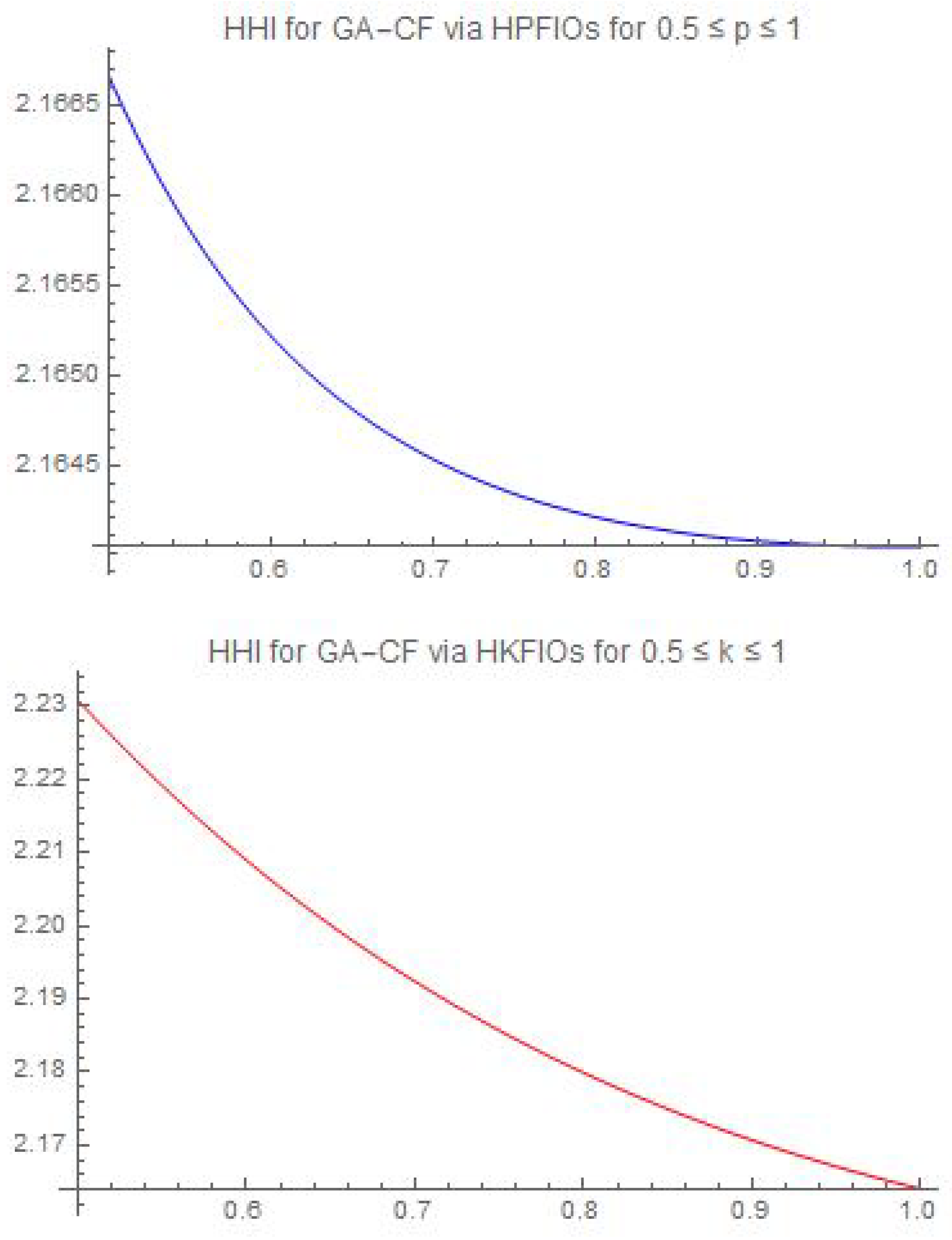
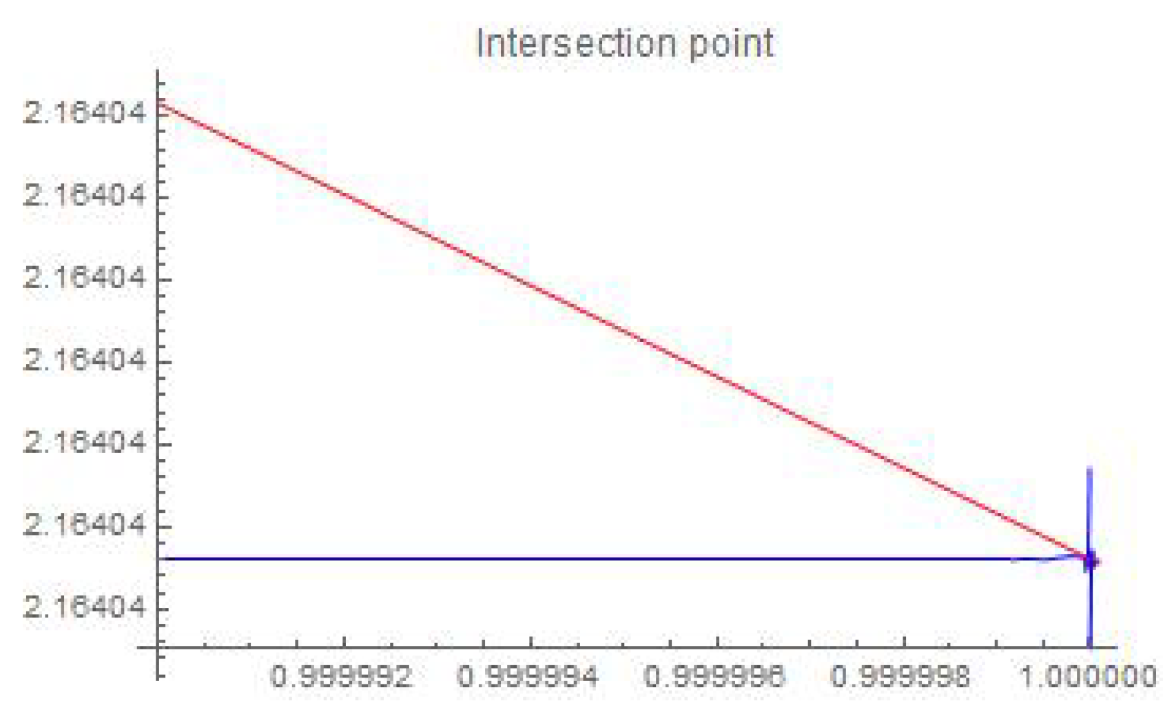
5. Comparison Between the Generalizations of Hermite–Hadamard–Mercer-Type Inequalities via GA-CFs via HPFIOs and HKFIOs

In this section, we compare two generalizations of the HHMI obtained via HPFIOs and HKFIOs. Note that the parameters contributing to generalizing the existing results are p and k in Section 3 and Section 4, respectively. So, in this section, we draw a comparison between generalizations by means of the obtained inequalities for different values of the parameter p and k. More specifically, we compare Corollary $3.4$ and Corollary $4.4$ by substituting a GA-CF and draw comparisons for p and k with ${\displaystyle \frac{1}{2}}\le p,k\le 1$.

Example 1.

For any GA-CF f, $=[\mu ,\nu ]=[1,2]$, $\tau =1$ the inequalities corresponding to the parameter p and k, obtained from Corollary $3.4$ and Corollary $4.4$ are

$$f\left(\sqrt{2}\right)\le \left[{\displaystyle \frac{p}{2\left\{ln\left(2\right)e^{\frac{p-1}{p}ln\left(2\right)}-\frac{p-1}{p}{\int }_1^{2}ln\left(\frac{2}{z}\right)e^{\frac{p-1}{p}ln\left(\frac{2}{z}\right)}\frac{dz}{z}\right\}}}\right]\left\{{𝚥}_{1+}^{1,p}f\left(2\right)+{𝚥}_{2-}^{1,p}f\left(1\right)\right\}\le {\displaystyle \frac{f\left(2\right)+f\left(1\right)}{2}}$$

(16)

and

$$f\left(\sqrt{2}\right)\le {\displaystyle \frac{1}{2{ln}^{\frac{1}{k}}\left(2\right)}}\left\{{𝚥}_{1+,k}^{1}f\left(2\right)+{𝚥}_{2-,k}^{1}f\left(1\right)\right\}\le {\displaystyle \frac{f\left(2\right)+f\left(1\right)}{2}}$$

(17)

Now, if we take $f\left(z\right)=z^2$, for $z\in [1,2]$. By page 156 of [25], the other meaning of GA convexity shows that a function f is GA-CF if $z^2{f}^{\left(2\right)}+z{f}^{\left(1\right)}\ge 0$, the function f is GA-CF. Therefore, by using (16) and (17), we construct the graphical comparisons for $f\left(z\right)=z^2$ corresponding to $0.5\le p,k\le 1$, as shown in Figure 1.

In addition, Figure 2 shows the difference between the expressions obtained via HPFIO and HKFIO. The result shows that the estimation obtained via HPFIOs is less than the HKFIOs.

Finally, both values coincide at $p=k=1$, as shown in Figure 3.

6. Applications

In this section, we present applications of the HHIs for GA-CFs obtained via HPFIOs and HKFIOs by establishing interpolation relations between the arithmetic mean and the geometric mean (AM-GM). Furthermore, we give a brief review of operator entropies and, by using Corollary $3.4$ and Corollary $4.4$, obtain upper bounds for the Tsallis relative operator entropy.

We use the notation for the generalized logarithmic function ${ln}_q\left(x\right):={\displaystyle \frac{x^{1-q}-1}{1-q}},(q\ne 1,x>0)$, which uniformly converges to the usual logarithmic function $logx$ as $q\to 1$. In the following theorem, we present applications of Corollary $3.4$ proved by using HPFIOs with the parameter $p\in (0,1]$.

Theorem 9.

Let $p\in (0,1]$ and $\mu ,\nu >0$.

(i) 

If $p\ne {\displaystyle \frac{1}{2}}$, then

$$\sqrt{\mu \nu }\le \left({\displaystyle \frac{1-p}{2}}\right)\left\{{\displaystyle \frac{\nu -{\mu }^{\frac{1}{p}}{\nu }^{1-\frac{1}{p}}}{1-{\mu }^{\frac{1}{p}-1}{\nu }^{1-\frac{1}{p}}}}+{\displaystyle \frac{\mu -{\mu }^{-1+\frac{1}{p}}{\nu }^{2-\frac{1}{p}}}{(1-2p)\left(1-{\mu }^{\frac{1}{p}-1}{\nu }^{1-\frac{1}{p}}\right)}}\right\}\le {\displaystyle \frac{\mu +\nu }{2}}.$$

(18)

(ii) 

$\sqrt{\mu \nu }\le {\displaystyle \frac{1}{2}}\left\{{\displaystyle \frac{\mu +\nu }{2}}+\mu \nu \left({\displaystyle \frac{log\nu -log\mu }{\nu -\mu }}\right)\right\}\le {\displaystyle \frac{\mu +\nu }{2}}.$

Proof. 

From Corollary 3.4 with $\tau =1$, we obtain

$$f\left(\sqrt{\mu \nu }\right){ln}_{1/p}\left({\displaystyle \frac{\nu }{\mu }}\right)\le {\displaystyle \frac{1}{2}}{\int }_{\mu }^{\nu }\left\{{\left({\displaystyle \frac{z}{\mu }}\right)}^{1-{\displaystyle \frac{1}{p}}}+{\left({\displaystyle \frac{\nu }{z}}\right)}^{1-{\displaystyle \frac{1}{p}}}\right\}{\displaystyle \frac{f\left(z\right)}{z}}dz\le \left({\displaystyle \frac{f\left(\mu \right)+f\left(\nu \right)}{2}}\right){ln}_{1/p}\left({\displaystyle \frac{\nu }{\mu }}\right)$$

(19)

for a GA–CF function and $\nu >\mu >0$. Since

$${\displaystyle \frac{1}{2}}{\int }_{\mu }^{\nu }\left\{{\left({\displaystyle \frac{z}{\mu }}\right)}^{1-{\displaystyle \frac{1}{p}}}+{\left({\displaystyle \frac{\nu }{z}}\right)}^{1-{\displaystyle \frac{1}{p}}}\right\}{\displaystyle \frac{logz}{z}}dz=log\left(\sqrt{\mu \nu }\right)\left({\displaystyle \frac{{\left(\frac{\nu }{\mu }\right)}^{1-\frac{1}{p}}-1}{1-\frac{1}{p}}}\right)=log\left(\sqrt{\mu \nu }\right){ln}_{1/p}\left({\displaystyle \frac{\nu }{\mu }}\right)$$

we confirm the equalities in the above inequalities when $f\left(z\right):=logz$.

If we take $f\left(z\right):=z$, then

$${\displaystyle \frac{1}{2}}{\int }_{\mu }^{\nu }\left\{{\left({\displaystyle \frac{z}{\mu }}\right)}^{1-{\displaystyle \frac{1}{p}}}+{\left({\displaystyle \frac{\nu }{z}}\right)}^{1-{\displaystyle \frac{1}{p}}}\right\}{\displaystyle \frac{f\left(z\right)}{z}}dz={\displaystyle \frac{p}{2}}\left(\nu \left(1-{\left({\displaystyle \frac{\nu }{\mu }}\right)}^{-1/p}\right)+{\displaystyle \frac{{\mu }^2-{\nu }^2{\left(\frac{\nu }{\mu }\right)}^{-1/p}}{\mu (1-2p)}}\right)$$

so that we obtain from (19) the relation (18). It is easy to see that

$$m_1(\mu ,\nu ):={\displaystyle \frac{\nu -{\mu }^{\frac{1}{p}}{\nu }^{1-\frac{1}{p}}}{1-{\mu }^{\frac{1}{p}-1}{\nu }^{1-\frac{1}{p}}}}\mathrm{and}{m}_2(\mu ,\nu ):={\displaystyle \frac{\mu -{\mu }^{-1+\frac{1}{p}}{\nu }^{2-\frac{1}{p}}}{1-{\mu }^{\frac{1}{p}-1}{\nu }^{1-\frac{1}{p}}}}$$

are symmetric by the simple calculations $m_1(\nu ,\mu )=m_1(\mu ,\nu )$ and $m_2(\nu ,\mu )=m_2(\mu ,\nu )$. Thus the relation (18) holds for all $\mu ,\nu >0$.

Finally, we have (ii) by taking $p:={\displaystyle \frac{1}{2}}$ with the limit $\underset{p\to {\displaystyle \frac{1}{2}}}{lim}{\displaystyle \frac{\mu -{\mu }^{-1+\frac{1}{p}}{\nu }^{2-\frac{1}{p}}}{1-2p}}=-2\mu log{\displaystyle \frac{\mu }{\nu }}$.

□

Remark 6.

(i) 

The inequalities (18) give the improved inequality for the arithmetic–geometric mean inequality. Letting $p\to 1$ above, we also obtain the known relation among the arithmetic mean, the geometric mean, and the logarithmic mean:

$$G(\mu ,\nu )\le L(\mu ,\nu )\le A(\mu ,\nu ),$$

(20)

where the arithmetic mean $A(\mu ,\nu ):={\displaystyle \frac{\mu +\nu }{2}}$, the geometric mean $G(\mu ,\nu ):=\sqrt{\mu }$ and the logarithmic mean $L(\mu ,\nu ):={\displaystyle \frac{\nu -\mu }{log\nu -log\mu }},(\mu \ne \nu )$ with $L(\mu ,\mu ):=\mu$, since we have $\underset{p\to 1}{lim}{\displaystyle \frac{1-p}{1-{\mu }^{\frac{1}{p}-1}{\nu }^{1-\frac{1}{p}}}}={\displaystyle \frac{1}{log\nu -log\mu }}$. Thus, the inequalities (18) give the new interpolation relation between the arithmetic mean and the geometric mean.

(ii) 

We easily find that

$$\mu \nu \left({\displaystyle \frac{log\nu -log\mu }{\nu -\mu }}\right)={\displaystyle \frac{log{\nu }^{-1}-log{\mu }^{-1}}{{\nu }^{-1}-{\mu }^{-1}}}=L{({\mu }^{-1},{\nu }^{-1})}^{-1}.$$

It is known that

$$A{({\mu }^{-1},{\nu }^{-1})}^{-1}\le L{({\mu }^{-1},{\nu }^{-1})}^{-1}\le G(\mu ,\nu )\le L(\mu ,\nu )\le A(\mu ,\nu ),$$

where $H(\mu ,\nu ):=A{({\mu }^{-1},{\nu }^{-1})}^{-1}$ is called the harmonic mean and $G{({\mu }^{-1},{\nu }^{-1})}^{-1}=G(\mu ,\nu )$. Then, $\left(ii\right)$ in Theorem 9 shows

$$2G(\mu ,\nu )-A(\mu ,\nu )\le L{({\mu }^{-1},{\nu }^{-1})}^{-1}\le A(\mu ,\nu ).$$

Although the second inequality is trivial, the first inequality is not trivial.

We give a brief review of relative operator entropies. A self–adjoint operator A acting on a Hilbert space $\mathcal{H}$ is called positive, and it is denoted by $A\ge 0$ if $\langle Ax,x\rangle \ge 0$ for any vector $x\in \mathcal{H}$. A self-adjoint operator A is called strictly positive and it is denoted by $A>0$ if A is positive and invertible. The order $A\ge B$ for two self–adjoint operators $A,B$ means $A-B\ge 0$. For two positive operators $A,B$, we denote

$$A{♯}_{q}B:=A^{1/2}{\left(A^{-1/2}B{A}^{-1/2}\right)}^q{A}^{1/2},q\in \mathbb{R}.$$

If $q\in [0,1]$, then $A{♯}_{q}B$ is called the operator geometric mean. For two positive operators $A,B$, the relative operator entropy $S\left(A\right|B)$ [41] and the Tsallis relative operator entropy $T_q\left(A\right|B)$ [42] are defined by

$$\begin{array}{cc}\hfill & S\left(A\right|B):=A^{1/2}log\left(A^{-1/2}B{A}^{-1/2}\right)A^{1/2}\hfill \\ \hfill & T_q\left(A\right|B):=A^{1/2}{ln}_q\left(A^{-1/2}B{A}^{-1/2}\right)A^{1/2}={\displaystyle \frac{A{♯}_{1-q}B-A}{1-q}},(q\ne 1).\hfill \end{array}$$

Note that $\underset{q\to 1}{lim}{T}_q\left(A\right|B)=S\left(A\right|B)$ by $\underset{q\to 1}{lim}{ln}_q\left(x\right)=logx$. See Section 7.3 of [43] and the references therein for recent results on the relative operator entropies. Applying the inequalities (19), we give upper bounds for the Tsallis relative operator entropy.

Theorem 10.

Let $p\in (0,1]$, and let $A,B$ be positive operators such that $A\le B$. Then,

(i) 

If $p\ne {\displaystyle \frac{1}{2}}$, then

$$\begin{array}{cc}\hfill T_{{\displaystyle \frac{1}{p}}}\left(A\right|B)& \le {\displaystyle \frac{p}{2}}\left(A{♯}_{{\displaystyle \frac{1}{2}}}B-A{♯}_{{\displaystyle \frac{1}{2}}-{\displaystyle \frac{1}{p}}}B+{\displaystyle \frac{1}{1-2p}}\left(A{♯}_{-{\displaystyle \frac{1}{2}}}B-A{♯}_{{\displaystyle \frac{3}{2}}-{\displaystyle \frac{1}{p}}}B\right)\right)\hfill \\ \hfill & \le \left({\displaystyle \frac{A{♯}_{\frac{1}{2}}B+A{♯}_{-\frac{1}{2}}B}{2}}\right)A^{-1}{T}_{{\displaystyle \frac{1}{p}}}\left(A\right|B).\hfill \end{array}$$

(ii) 

$T_2\left(A\right|B)\le {\displaystyle \frac{1}{4}}\left(A{♯}_{{\displaystyle \frac{1}{2}}}B-A{♯}_{-{\displaystyle \frac{3}{2}}}B\right)+{\displaystyle \frac{1}{2}}S\left(A\right|B)\le \left({\displaystyle \frac{A{♯}_{\frac{1}{2}}B+A{♯}_{-\frac{1}{2}}B}{2}}\right)A^{-1}{T}_2\left(A\right|B).$

Proof. 

Putting $f\left(z\right):=z$ and $\mu :=1$ in the inequalities (19), we obtain

$$\sqrt{\nu }{ln}_{{\displaystyle \frac{1}{p}}}\nu \le {\displaystyle \frac{p}{2}}\left(\nu -{\nu }^{1-{\displaystyle \frac{1}{p}}}+{\displaystyle \frac{1-{\nu }^{2-\frac{1}{p}}}{1-2p}}\right)\le \left({\displaystyle \frac{\nu +1}{2}}\right){ln}_{{\displaystyle \frac{1}{p}}}\nu ,\left(\nu \ge 1,p\ne {\displaystyle \frac{1}{2}}\right)$$

(21)

which implies

$${ln}_{{\displaystyle \frac{1}{p}}}\nu \le {\displaystyle \frac{p}{2}}\left({\nu }^{{\displaystyle \frac{1}{2}}}-{\nu }^{{\displaystyle \frac{1}{2}}-{\displaystyle \frac{1}{p}}}+{\displaystyle \frac{{\nu }^{-\frac{1}{2}}-{\nu }^{\frac{3}{2}-\frac{1}{p}}}{1-2p}}\right)\le \left({\displaystyle \frac{{\nu }^{\frac{1}{2}}+{\nu }^{-\frac{1}{2}}}{2}}\right){ln}_{{\displaystyle \frac{1}{p}}}\nu ,\left(p\ne {\displaystyle \frac{1}{2}}\right).$$

Putting $\nu :=A^{-1/2}B{A}^{-1/2}\ge 1$ with the standard functional calculus and multiplying $A^{1/2}$ from both sides, we obtain (i).

If we take the limit $p\to {\displaystyle \frac{1}{2}}$ in (21), we have

$${ln}_2\nu \le {\displaystyle \frac{1}{4}}\left({\nu }^{{\displaystyle \frac{1}{2}}}-{\nu }^{-{\displaystyle \frac{3}{2}}}\right)+{\displaystyle \frac{1}{2}}log\nu \le \left({\displaystyle \frac{{\nu }^{\frac{1}{2}}+{\nu }^{-\frac{1}{2}}}{2}}\right){ln}_2\nu$$

since $\underset{p\to {\displaystyle \frac{1}{2}}}{lim}\left({\displaystyle \frac{1-{\nu }^{2-\frac{1}{p}}}{1-2p}}\right)=2log\nu$. Thus, we obtain (ii) in a similar way to the above. □

If we take $p:=1$ in Theorem 10, then we have the upper bound of the relative operator entropy

$$S\left(A\right|B)\le A{♯}_{{\displaystyle \frac{1}{2}}}B-A{♯}_{-{\displaystyle \frac{1}{2}}}B\le \left({\displaystyle \frac{A{♯}_{\frac{1}{2}}B+A{♯}_{-\frac{1}{2}}B}{2}}\right)A^{-1}S\left(A\right|B)$$

for $0\le A\le B$.

Now, we present the applications of Corollary $4.4$ obtained via HKFIOs with the parameter $k>0$. If we take $f\left(z\right):=z$ and $\tau :=1$ in Corollary $4.4$, then for $\nu >\mu >0$,

$$\sqrt{\mu \nu }\le {\displaystyle \frac{{\Gamma }_k\left(2\right)}{2k{\Gamma }_k\left(1\right){\left(log\nu -log\mu \right)}^{1/k}}}{\int }_{\mu }^{\nu }\left\{{\left(log{\displaystyle \frac{\nu }{z}}\right)}^{{\displaystyle \frac{1}{k}}-1}+{\left(log{\displaystyle \frac{z}{\mu }}\right)}^{{\displaystyle \frac{1}{k}}-1}\right\}dz\le {\displaystyle \frac{\mu +\nu }{2}},$$

(22)

which also gives a new interpolational relation on the generalized logarithmic mean between the arithmetic mean and the geometric mean. We easily find that the above relation recovers (20) when $k:=1$. Here, the Gamma k-function ${\Gamma }_k\left(\alpha \right)$ [10] for $k>0$ is defined as

$${\Gamma }_k\left(\alpha \right):={\int }_0^{\infty }{t}^{\alpha -1}exp\left(-{\displaystyle \frac{t^k}{k}}\right)dt,\mathrm{Re}\left(\alpha \right)>0.$$

However the calculations of the integrals in (22) are quite complicated. By using the computer software Mathematica version 8 [44], we obtain

$$\begin{array}{cc}\hfill & {\int }_{\mu }^{\nu }\left\{{\left(log\frac{\nu }{z}\right)}^{\frac{1}{k}-1}+{\left(log\frac{z}{\mu }\right)}^{\frac{1}{k}-1}\right\}dz\hfill \\ \hfill & =\left({(-1)}^{\frac{1}{k}}\mu +\nu \right)\Gamma \left(\frac{1}{k}\right)-\nu \Gamma \left(\frac{1}{k} ,log\frac{\nu }{\mu }\right)-\mu E_{1-\frac{1}{k}}\left(-log\frac{\nu }{\mu }\right){\left(log\nu -log\mu \right)}^{1/k},\hfill \end{array}$$

where

$$\Gamma (a,z):={\int }_z^{\infty }{t}^{a-1}{e}^{-t}dt,E_n\left(z\right):={\int }_1^{\infty }{t}^{-n}{e}^{-zt}dt.$$

We take $\tau =k$ in Corollary 4.4. Then,

$$f\left(\sqrt{\mu \nu }\right)\le {\displaystyle \frac{{\Gamma }_k(k+1)}{2k{\Gamma }_k\left(k\right)\left(log\nu -log\mu \right)}}{\int }_{\mu }^{\nu }{\displaystyle \frac{2f\left(z\right)}{z}}dz\le {\displaystyle \frac{f\left(\mu \right)+f\left(\nu \right)}{2}},$$

which gives

$$\sqrt{\mu \nu }\le {\displaystyle \frac{{\Gamma }_k\left(1\right)(\nu -\mu )}{k(log\nu -log\mu )}}\le {\displaystyle \frac{\mu +\nu }{2}},(k>0,\nu >\mu >0)$$

when $f\left(z\right):=z$ since ${\Gamma }_k\left(k\right)=1$ and ${\Gamma }_k(k+1)={\Gamma }_k\left(1\right)$. (See [10].) Since ${\Gamma }_k\left(1\right)=k^{{\displaystyle \frac{1}{k}}}\Gamma \left(1+{\displaystyle \frac{1}{k}}\right)=k^{{\displaystyle \frac{1}{k}}}\times {\displaystyle \frac{1}{k}}\Gamma \left({\displaystyle \frac{1}{k}}\right)$, the above relation is rewritten as

$$\sqrt{\mu \nu }\le k^{{\displaystyle \frac{1}{k}}-2}\Gamma \left(k^{-1}\right)\left({\displaystyle \frac{\nu -\mu }{log\nu -log\mu }}\right)\le {\displaystyle \frac{\mu +\nu }{2}},(k>0,\nu >\mu >0).$$

However, the above inequalities do not hold in general since $\underset{k\to \infty }{lim}{k}^{{\displaystyle \frac{1}{k}}-2}\Gamma \left(k^{-1}\right)=0$.

7. Conclusions

Motivated by the applicability of fractional calculus, mathematical inequalities, derived families of convex functions, and information sciences, we have investigated these topics together. The findings of this paper cover (i) generalizations in terms of multiple aspects and the unification of main results from [6,7,37,38], (ii) the comparison between new generalizations, and (iii), most importantly, applications to information sciences and interpolating means. Unlike the common development in mathematical inequalities, the current results not only cover the theoretical aspects but also provide comparisons between inequalities and applications. The applications of newly proved HHIs for GA-CFs obtained via HPFIOs and HKFIOs in determining interpolation relations between AM-GM and upper bounds for the Tsallis relative operator entropy is a distinct feature of this study.

References

1. Kai, D. The analysis of fractional differential equations: An application-oriented exposition using differential operators of Caputo type. In Lecture Notes in Mathematics; Springer: Berlin/Heidelberg, Germany, 2004. [Google Scholar]
2. Alshammari, S.; Alshammari, M.; Alabedalhadi, M.; Al-Sawalha, M.M.; Al-Smadi, M. Numerical investigation of a fractional model of a tumor-immune surveillance via Caputo operator. Alex. Eng. J. 2024, 86, 525–536. [Google Scholar] [CrossRef]
3. Ferrari, A.L.; Gomes, M.C.S.; Aranha, A.C.R.; Paschoal, S.M.; de Souza, M.G.; de Matos, J.L.M.; Defendi, R.O. Mathematical modeling by fractional calculus applied to separation processes. Sep. Purif. Technol. 2024, 337, 126310. [Google Scholar] [CrossRef]
4. Set, E.; Kashuri, A.; Mumcu, I. Chebyshev type inequalities by using generalized proportional Hadamard fractional integrals via Polya–Szegö inequality with applications. Chaos Solitons Fractals 2021, 146, 110860. [Google Scholar] [CrossRef]
5. Kilbas, A.A.; Srivastava, H.M.; Trujillo, J.J. Theory and Applications of Fractional Differential Equations; Elsevier: Amsterdam, The Netherlands, 2006; Volume 204. [Google Scholar]
6. Fahad, A.; Ayesha; Wang, Y.; Butt, S.I. Jensen–Mercer and Hermite–Hadamard–Mercer Type Inequalities for GA-h-Convex Functions and Its Subclasses with Applications. Mathematics 2023, 11, 278. [Google Scholar] [CrossRef]
7. Iscan, I. Jensen—Mercer inequality for GA-convex functions and some related inequalities. J. Inequalities Appl. 2020, 212, 212. [Google Scholar] [CrossRef]
8. Rahman, G.; Abdeljawad, T.; Jarad, F.; Khan, A.; Nisar, K.S. Certain inequalities via generalized proportional Hadamard fractional integral operators. Adv. Differ. Equ. 2019, 2019, 454. [Google Scholar] [CrossRef]
9. Gambo, Y.Y.; Jarad, F.; Baleanu, D.; Abdeljawad, T. On Caputo modification of the Hadamard fractional derivatives. Adv. Differ. Equ. 2014, 2014, 10. [Google Scholar] [CrossRef]
10. Iqbal, S.; Mubeen, S.; Tomar, M. On Hadamard k-fractional integrals. J. Fract. Calc. Appl. 2018, 9, 255–267. [Google Scholar]
11. Tarasov, V.E. Entropy interpretation of Hadamard type fractional operators: Fractional cumulative entropy. Entropy 2022, 24, 1852. [Google Scholar] [CrossRef]
12. Todinov, M. Reverse Engineering of Algebraic Inequalities for System Reliability Predictions and Enhancing Processes in Engineering. IEEE Trans. Reliab. 2023, 73, 902–911. [Google Scholar] [CrossRef]
13. Huang, J.; Luo, D. Relatively exact controllability for higher-order fractional stochastic delay differential equations. Inf. Sci. 2023, 648, 119631. [Google Scholar] [CrossRef]
14. Aydin, F. Boundary-aware local Density-based outlier detection. Inf. Sci. 2023, 647, 119520. [Google Scholar] [CrossRef]
15. Akhtar, N.; Awan, M.U.; Javed, M.Z.; Rassias, M.T.; Mihai, M.V.; Noor, M.A.; Noor, K.I. Ostrowski type inequalities involving harmonically convex functions and applications. Symmetry 2021, 13, 201. [Google Scholar] [CrossRef]
16. Khan, Z.A.; Afzal, W.; Nazeer, W.; Asamoah, J.K.K. Some New Variants of Hermite–Hadamard and Fejér-Type Inequalities for Godunova–Levin Preinvex Class of Interval-Valued Functions. J. Math. 2024, 2024, 8814585. [Google Scholar] [CrossRef]
17. Mohammed, P.O.; Abdeljawad, T.; Alqudah, M.A.; Jarad, F. New discrete inequalities of Hermite–Hadamard type for convex functions. Adv. Differ. Equ. 2021, 2021, 122. [Google Scholar] [CrossRef]
18. Srivastava, H.M.; Sahoo, S.K.; Mohammed, P.O.; Baleanu, D.; Kodamasingh, B. Hermite–Hadamard type inequalities for interval-valued preinvex functions via fractional integral operators. Int. J. Comput. Intell. Syst. 2022, 15, 8. [Google Scholar] [CrossRef]
19. Huy, D.Q.; Van, D.T.T. Some inequalities for convex functions and applications to operator inequalities. Asian-Eur. J. Math. 2023, 16, 2350216. [Google Scholar] [CrossRef]
20. Yang, W. Certain new weighted Young and Polya Szego-type inequalities for unified fractional inegral operators via an extended generalized Mittag-Leffler function with applications. Fractals 2022, 30, 2250106. [Google Scholar] [CrossRef]
21. Beckenbach, E.F. Convex functions. Bull. Am. Math. Soc. 1948, 54, 439–460. [Google Scholar] [CrossRef]
22. Noor, M.A.; Noor, K.I.; Rassias, M.T. Characterizations of higher order strongly generalized convex functions. Nonlinear Anal. Differ. Equ. Appl. 2021, 341–364. [Google Scholar]
23. Luo, C.; Wang, H.; Du, T. Fejér—Hermite—Hadamard type inequalities involving generalized h-convexity on fractal sets and their applications. Chaos Solitons Fractals 2020, 131, 109547. [Google Scholar] [CrossRef]
24. Mihai, M.V.; Noor, M.A.; Noor, K.I.; Awan, M.U. Some integral inequalities for harmonic h-convex functions involving hypergeometric functions. Appl. Math. Comput. 2015, 252, 257–262. [Google Scholar] [CrossRef]
25. Niculescu, C.P. Convexity according to the geometric mean. Math. Inequal. Appl. 2000, 3, 155–167. [Google Scholar] [CrossRef]
26. Latif, M.A.; Dragomir, S.S.; Momoniat, E. Some Fejér type integral inequalities for geometrically-arithmetically-convex functions with applications. Filomat 2018, 32, 2193–2206. [Google Scholar] [CrossRef]
27. Noor, M.A.; Noor, K.I.; Awan, M.U. Some inequalities for geometricallyarithmetically h-convex functions. Creat. Math. Inform 2014, 23, 91–98. [Google Scholar] [CrossRef]
28. Fahad, A.; Wang, Y.; Ali, Z.; Hussain, R.; Furuichi, S. Exploring properties and inequalities for geometrically arithmetically-Cr-convex functions with Cr-order relative entropy. Inf. Sci. 2024, 662, 120219. [Google Scholar] [CrossRef]
29. Fahad, A.; Ali, Z.; Furuichi, S.; Wang, Y. Novel fractional integral inequalities for GA-Cr-convex functions and connections with information systems. Alex. Eng. J. 2025, 113, 509–515. [Google Scholar] [CrossRef]
30. Dragomir, S.S.; Pearce, C. Selected Topics on Hermite–Hadamard Inequalities and Applications. Science Direct Working Paper No S1574-0358(04)70845-X. Available online: https://ssrn.com/abstract=3158351 (accessed on 14 October 2024).
31. Ozdemir, M.E.; Ragomir, S.S.; Yildiz, C. The Hadamard inequality for convex function via fractional integrals. Acta Math. Sci. 2013, 33, 1293–1299. [Google Scholar] [CrossRef]
32. Sun, W.; Liu, Q. Hadamard type local fractional integral inequalities for generalized harmonically convex functions and applications. Math. Methods Appl. Sci. 2020, 43, 5776–5787. [Google Scholar] [CrossRef]
33. Sun, W. Some new inequalities for generalized h-convex functions involving local fractional integral operators with Mittag-Leffler kernel. Math. Methods Appl. Sci. 2021, 44, 4985–4998. [Google Scholar] [CrossRef]
34. Vivas, M.; Hernández, J.; Merentes, N. New Hermite–Hadamard and Jensen type inequalities for h-convex functions on fractal sets. Rev. Colomb. MatemáTicas 2016, 50, 145–164. [Google Scholar] [CrossRef]
35. Chen, J.; Luo, C. Certain generalized Riemann–Liouville fractional integrals inequalities based on exponentially (h, m)-preinvexity. J. Math. Anal. Appl. 2024, 530, 127731. [Google Scholar] [CrossRef]
36. Du, T.; Peng, Y. Hermite–Hadamard type inequalities for multiplicative Riemann–Liouville fractional integrals. J. Comput. Appl. Math. 2024, 440, 115582. [Google Scholar] [CrossRef]
37. Iscan, I. New general integral inequalities for quasi-geometrically convex functions via fractional integrals. J. Inequal. Appl. 2013, 491. [Google Scholar] [CrossRef]
38. Kunt, M.; Iscan, I. Fractional Hermite–Hadamard–Fejér type inequalities for GA-convex functions. Turk. J. Inequal. 2018, 2, 1–20. [Google Scholar]
39. Pachpatte, B.G. Integral and Finite Difference Inequalities and Applications; Elsevier: Amsterdam, The Netherlands, 2006. [Google Scholar]
40. Varosanec, S. On h-convexity. J. Math. Anal. Appl. 2007, 326, 303–311. [Google Scholar] [CrossRef]
41. Fujii, J.I. Relative operator entropy in noncommutative information theory. Math. Jpn. 1990, 35, 387–396. [Google Scholar]
42. Yanagi, K.; Kuriyama, K.; Furuichi, S. Generalized Shannon inequalities based on Tsallis relative operator entropy. Linear Algebra Its Appl. 2005, 394, 109–118. [Google Scholar] [CrossRef]
43. Furuichi, S. Advances in Mathematical Inequalities; Walter de Gruyter GmbH Co KG: Berlin, Germany, 2020. [Google Scholar]
44. A Scientific and Technical Computing System Developed by Wolfram Research. Available online: https://www.wolfram.com/mathematica (accessed on 14 October 2024).
Figure 1. HHI for f ( z ) = z 2 bounded below by 2 and above by 2.5 with respect to the parameters p and k.
Fractalfract 08 00728 g001
Figure 2. Difference between the HHI obtained via HPFIOs and HKFIOs.
Fractalfract 08 00728 g002
Figure 3. HPFIOs and HKFIOs coincide.
Fractalfract 08 00728 g003
Disclaimer/Publisher’s Note: The statements, opinions and data contained in all publications are solely those of the individual author(s) and contributor(s) and not of MDPI and/or the editor(s). MDPI and/or the editor(s) disclaim responsibility for any injury to people or property resulting from any ideas, methods, instructions or products referred to in the content.