Variable Time Step Algorithm for Transient Response Analysis for Control and Optimization

Abstract

This work considers an optimization problem based on step response characteristics. We lay a foundation for it by designing a rapid transient response analysis algorithm with variable time steps. This method applies to linear ordinary differential equations with real order. Numerical tests of the algorithm in the integer case show significant improvement even for higher order systems. This suggests a new method for acquiring step response characteristics for the fractional order case for which we have constructed an explicit expression of the inverse Laplace transform.

1. Introduction

This paper deals with the computer-aided analysis of transient responses. We aim to support optimization problems connected with the design process of control systems. Such systems may have multiple variable parameters both in the structure and the controller. These optimization problems often rely on estimating output signals. An improvement in the calculation time at this step improves the overall efficiency of the chosen optimization strategy. This research describes an algorithm for acquiring step response characteristics. It provides additional speed by implementing novel strategies for choosing the size of the variable time step. This method is based on explicit inverse Laplace transform expressions, which are crucial for faster step response analysis. We are going to test the developed algorithm in comparison with standard computer-aided means of transient response analysis like Matlab. Another point of interest is the fact that most of the available programs for step response analysis do not support fractional order systems. So, differential equations with powers of derivatives that are real non-integer numbers are not suitable for these programs. In order to apply the developed algorithm in this case, we have acquired an explicit expression for the inverse Laplace transform of a feedback control system with a fractional order controller. No reduction or approximation techniques are required to use the developed method.

There are a few programs for determining step response characteristics. Quite often, they are part of major mathematical software like Matlab (current version is 2024b), Mathematica (current version is 14.1.0), Maple (current version is 2024.2), etc. The fastest and most notable is Matlab’s Control System Toolbox, which provides algorithms for the design and tuning of linear control systems [1]. It has tools to work with both frequency domain and state-space methods. The validation of the design is possible by verifying step response characteristics like overshoot, settling time, rise time, etc. However, this toolbox is suited for integer-order differential equations. This means that the powers of derivatives in these equations are positive integers. In case of a fractional order system, one has to refer to various toolboxes created by independent researches.

Fractional calculus is an evolving field of mathematics. There are different ways one can define a real or a complex power of a differential operator [2]. In the course of research and development of fractional calculus, it was established that a fractional-order derivative must satisfy a few conditions. It should be a linear operator and, if an integer was chosen as a power for a real-order derivative, it must yield the same result as an integer derivative would [3]. Some other properties like the index law or the Leibniz rule must be met as well. The first fractional derivatives that satisfy these conditions are the Riemann–Liouville and the Grunwald–Letnikov types [4,5,6].

Some physical phenomena are better described using mathematical models based on fractional derivatives and integrals [7]. A process under consideration is usually not isolated and may be affected by external perturbation forces. Therefore, integer operators may be inadequate for describing the trajectories of state variables. Fractional operators have a continuous set of derivative orders to choose, so there is room for optimization. The approximation of experimental data with different algorithms has proven to be more effective in various phenomena [8,9].

Classic control theory relies heavily on the second-order approximation. Higher order integer systems are quite often modeled this way [10]. Such an approximation provides explicit formulas for main step response characteristics like overshoot or settling time [11]. Similar efforts were found in the fractional-order case—it can be shown that for some dynamic systems, overshoot is unavoidable [12]. The authors in [12] have studied a certain class of fractional-order systems having commensurate orders between 1 and 2. An analytical inverse Laplace transformation of a fractional-order transfer function may present a challenge. Single-order transfer functions of this type are studied in [13].

A fractional-order linear quadratic regulator was created in [14] for controlling the current through a magnetic levitation system. For the state feedback law, a fractional-order state observer was constructed to estimate all of the states. The stabilization of a magnetic levitation system using a fractional-order proportional–integral–derivative (PID) controller, a fractional-order sliding mode, and fuzzy control approaches were compared and combined in [15].

The tuning of a closed-loop proportional–integral controller coupled with a single-order-time-delay fractional-order system is studied in [16]. The tuning was based on the root locus analysis. One and two degree-of-freedom fractional order PID controllers were designed in [17], both in simulation and real time. The design of such a controller requires the determination of five parameters, which was framed as an optimization problem. Dominant poles were identified based on the chosen transient response characteristics. The cost function was then formulated from the characteristic equation of the closed-loop system at those poles. A study on fractional-order PID controllers and curve-fitting approximations of their parameters is given in [18]. This work also provides real-time examples of process plants using such control strategies and approximation techniques.

Fractional-order calculus, while powerful in theory, sees limited applications. One of the reasons is the necessity of becoming familiar with different concepts and finding the right software. There are special programs for fractional-order modeling and control, mainly in Matlab. The authors in [19] created a Matlab toolbox for processing experimental data with the main focus on user accessibility. A system identification algorithm is used to obtain a model as a second-order plus dead-time system. A fractional-order PID controller is computed based on this estimation and some preset performance specifications.

The CRONE controller is one of the first fractional-order controllers for dynamic systems [20] which has seen various applications. The CRONE toolbox is capable of fractional-order modeling, system design, and identification. While certain steps were made for automating this process, a good deal of learning is required to successfully implement this strategy. A few strategies for multiple-input multiple-output systems are available as well.

The FOMCON open source toolbox for Matlab analyzes fractional-order transfer functions in a classical form of a polynomial divided by a polynomial. It is connected to the FOTF (Fractional-Order Transfer Functions) Matlab toolbox, which is also open source [21]. This toolbox has both time and frequency domain identification of fractional-order systems, as well as approximation methods and means for fractional-order PID control [22]. With its GUI and active support by the creators it is now, arguably, the best fractional-order toolbox for Matlab.

Other important mentions include the Ninteger toolbox for Matlab, which focuses on approximations of non-integer-order derivatives [23,24]. It has many pre-coded formulas for fractional-order PID and a couple of generations of CRONE controllers. FLOreS is a developing toolbox which focuses on the design of fractional-order controllers using loop-shaping [25]. This provides a graphical approach using special closed-loop sensitivity functions.

In this work we have created an algorithm capable of rapid step response analysis. The structure of the paper is as follows: Section 2 describes the optimization problem we aim to assist with our method. It also lists the dynamic systems under consideration both in the integer- and fractional-order cases. Section 3 presents a full description of the developed algorithm with a diagram and comments about the inner workings of the variable time step approach. Section 4.1 presents numerical tests which showcase the advantage of the designed method. Section 4.2 is an extension of the developed approach for a particular type of fractional-order system for which we have acquired an explicit expression for the inverse Laplace transform.

2. Materials and Methods

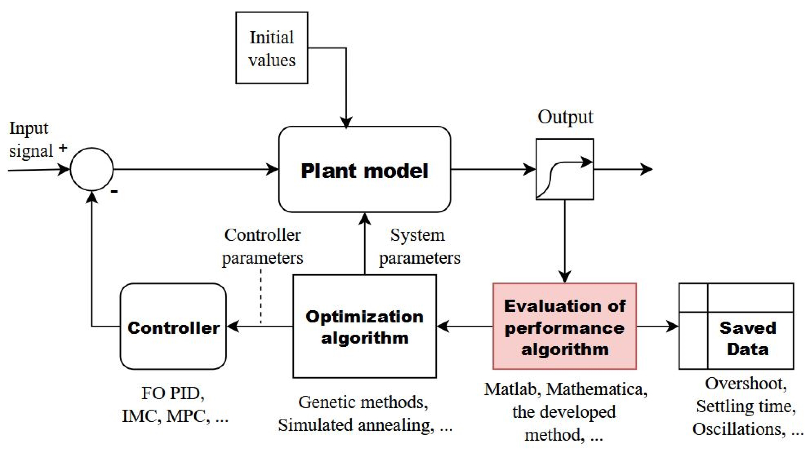
2.1. Problem Statement

Consider an engineering system under design (see Figure 1). The plant has a set of internal parameters, $\overrightarrow{\chi }=({\chi }_1,{\chi }_2,\dots ,{\chi }_n),{\chi }_i\in X$, the controller has its defining values, $\overrightarrow{\omega }=({\omega }_1,{\omega }_2,\dots ,{\omega }_m),{\omega }_j\in \Omega$, and the output is measured as a set of characteristics, $\overrightarrow{\eta }=({\eta }_1,{\eta }_2,\dots ,{\eta }_p),{\eta }_k\in H$, where $X,\Omega$ and $H\in \mathbb{R}$ are feasible sets. The optimization problem under consideration is to minimize an objective function which depends on the output characteristics $f\left(\overrightarrow{\eta }\right)$; for example, a weighed sum

$$f\left(\overrightarrow{\eta }\right)={\alpha }_1{\eta }_1^{k_1}+{\alpha }_2{\eta }_2^{k_2}+\cdots +{\alpha }_p{\eta }_p^{k_p},$$

where ${\alpha }_i\in \mathbb{R},i=1,2,\dots ,p$ are real numbers and $k_i>0.$ At the same time, since the output vector depends on $\overrightarrow{\chi }$ and $\overrightarrow{\omega },$ we can write it as a vector function $\overrightarrow{\eta }=\overrightarrow{\eta }(\overrightarrow{\chi },\overrightarrow{\omega }).$ Then, the optimization problem is

$$minf\left(\overrightarrow{\eta }\right)\equiv \underset{\overrightarrow{\chi }\in X,\overrightarrow{\omega }\in \Omega }{min}f\left(\overrightarrow{\eta }(\overrightarrow{\chi },\overrightarrow{\omega })\right).$$

(1)

A chosen optimization algorithm $\Phi$ (usually formulated as a set of rules; for example, simulated annealing [26]) would have the output characteristics $\overrightarrow{\eta }$ as the input and an $(1\times (n+m\left)\right)$ vector $\overrightarrow{r}=(\overrightarrow{\chi },\overrightarrow{\omega })$ as the output, so

$$\overrightarrow{r}=(\overrightarrow{\chi },\overrightarrow{\omega })=({\chi }_1,{\chi }_2,\dots ,{\chi }_n,{\omega }_1,{\omega }_2,\dots ,{\omega }_m)=\Phi \left(\overrightarrow{\eta }\right)=\Phi \left(\overrightarrow{\eta }(\overrightarrow{\chi },\overrightarrow{\omega })\right).$$

The choice of $\Phi$ depends on different factors, is a subject of research, and is discussed in various sources [27,28,29,30,31]. Here we shall focus on the foundation of such a problem—obtaining the vector $\overrightarrow{\eta }.$ Particularly, we are going to consider step response analysis.

If we look at Figure 1, we see that an increase in speed at this part speeds up the solution of the whole optimization problem. Later, we are going to show that standard computational methods and algorithms for step response analysis can be improved.

2.2. Control Systems Under Consideration

A model of a physical process is often represented as a system of ordinary differential equations (ODEs). The classical approach involves converting this system to a transfer function. Such an operation involves a certain integral transformation like the Laplace or the Z-transform. This algebraically relates the system model to the complex images of both input and output signals. Replacing a differential equation with an algebraic expression simplifies the modeling of interconnected systems. State-space methods (also known as the time-domain approach [11]) can achieve the same results. However, these methods apply to multiple-input multiple-output systems and enhance the capabilities of closed-loop feedback control. State-space methods can be used to represent nonlinear systems that have backlash, saturation, and dead zones, while easily handling nonzero initial conditions.

2.2.1. Integer-Order Dynamic Systems

In this work, we consider linear time-invariant systems. As for the integer case, a common single-input single-output system is

$$\begin{array}{c}{\displaystyle \frac{d^{n}y}{d{t}^n}}+a_{n-1}{\displaystyle \frac{d^{n-1}y}{d{t}^{n-1}}}+a_{n-2}{\displaystyle \frac{d^{n-2}y}{d{t}^{n-2}}}+\cdots +a_1{\displaystyle \frac{dy}{dt}}+a_0\\ =b_{0}u\left(t\right)+b_1{u}^{\prime }\left(t\right)+b_2{u}^{″}\left(t\right)+\cdots +b_{n-1}{u}^{(n-1)}\left(t\right).\end{array}$$

(2)

After applying the Laplace transformation, this equation has a transfer function of

$$H\left(s\right)={\displaystyle \frac{C\left(s\right)}{R\left(s\right)}}={\displaystyle \frac{b_{n-1}{s}^{n-1}+\cdots +b_{1}s+b_0}{s^n+a_{n-1}{s}^{n-1}+\cdots +a_{1}s+a_0}},$$

(3)

where s is a complex variable and both $a_0,a_1,\dots ,a_{n-1}$ and $b_0,b_1,\dots ,b_{n-1}$ are real numbers. It is a relation between the systems input $R\left(s\right)$ and output $C\left(s\right)$ complex images, if one was to obtain them via a Laplace transformation. This allows us to look at Equation (2) as a subsystem, so a connection of two subsystems, $H\left(s\right)$ and $T\left(s\right)$, results in a simple multiplication $H\left(s\right)T\left(s\right)$. In order to obtain a time domain signal, one has to perform an inverse Laplace transform, which in many cases may be quite difficult. However, for (3), it comes down to a simple partial fraction expansion [32].

An alternative way to deal with Equation (2) is to rewrite it with a matrix representation via state space. The components of vector $\overrightarrow{x}\left(t\right)$ are referred to as state variables. The function $u\left(t\right)$ is the input, while $y\left(t\right)$ is the system’s output. State variables are linear combinations of the output function $y\left(t\right)$ and its derivatives. They can be chosen in an infinite amount of ways. Quite often, it is

$$x_1\left(t\right)=y\left(t\right),x_2\left(t\right)=y^{\prime }\left(t\right),x_3\left(t\right)=y^{″}\left(t\right),\dots x_n\left(t\right)=y^{(n-1)}\left(t\right).$$

In a general case this choice of state variables $\overrightarrow{x}$ results in

$$\begin{array}{c}\hfill \dot{\overrightarrow{x}}\left(t\right)=A\overrightarrow{x}\left(t\right)+B\overrightarrow{u}\left(t\right),\hfill \\ \hfill \overrightarrow{y}\left(t\right)=C\overrightarrow{x}\left(t\right)+D\overrightarrow{u}\left(t\right),\hfill \end{array}$$

(4)

where $\overrightarrow{x}\in {\mathbb{R}}^{1\times n}$ is a vector containing the state variables, $\overrightarrow{y}\in {\mathbb{R}}^{1\times p}$ is the output vector, $\overrightarrow{u}\in {\mathbb{R}}^{1\times r}$ is the input vector, and $A\in {\mathbb{R}}^{n\times n}$, $B\in {\mathbb{R}}^{n\times r}$, $C\in {\mathbb{R}}^{p\times n}$, $D\in {\mathbb{R}}^{p\times r}$ are corresponding matrices. Then, the Equation (2) or, equally, the transfer function (3) is represented by what is called a controller canonical form (CCF) as follows:

$$\begin{array}{c}\dot{\overrightarrow{x}}\left(t\right)=A_{CCF}\overrightarrow{x}\left(t\right)+B_{CCF}u\left(t\right),\hfill \\ y\left(t\right)=C_{CCF}\overrightarrow{x}\left(t\right),\hfill \end{array}$$

(5)

where

$$A_{CCF}=\left(\begin{array}{cccccc}0& 1& 0& \cdots & 0& 0\\ 0& 0& 1& \cdots & 0& 0\\ ⋮& ⋮& ⋮& \ddots & ⋮& ⋮\\ 0& 0& 0& \cdots & 0& 0\\ 0& 0& 0& \cdots & 1& 0\\ 0& 0& 0& \cdots & 0& 1\\ -a_0& -a_1& -a_2& \cdots & -a_{n-2}& -a_{n-1}\end{array}\right);B_{CCF}=\left(\begin{array}{c}0\\ 0\\ ⋮\\ 0\\ 0\\ 0\\ 1\end{array}\right);$$

(6)

and $C_{CCF}=(b_0,b_1,b_2,\dots ,b_{n-2},b_{n-1}).$

The solution of the linear time-invariant state Equation (5) and (6) is known [11] to be

$$\overrightarrow{x}\left(t\right)=e^{A_{CCF}t}\overrightarrow{x_0}+e^{A_{CCF}t}{\int }_0^t{e}^{A_{CCF}\tau }{B}_{CCF}u\left(\tau \right)d\tau ,y\left(t\right)=C_{CCF}\overrightarrow{x},$$

(7)

where $\overrightarrow{x_0}\in {\mathbb{R}}^{1\times n}$ is a vector of initial values of state variables. The expression $e^{A_{CCF}t}$ is called the state transition matrix or matrix exponent and is defined as

$$e^{A_{CCF}t}=I+A_{CCF}t+{\displaystyle \frac{A_{CCF}^2{t}^2}{2!}}+{\displaystyle \frac{A_{CCF}^3{t}^3}{3!}}+\dots ,$$

where I is a $n\times n$ unit square matrix.

Expression (7) allows one to acquire an explicit expression of the steady state signal value. Consider the input to be a step function $u\left(t\right)=K{u}_s\left(t\right),$ where $K\in \mathbb{R}$ and $u_s\left(t\right)$ is a Heaviside step function. If we substitute this input to (7), it can be shown [33] that if A is non-singular and does not have an eigenvalue equal to zero, the steady state reaches a constant value $x_{ss}$ and $y_{ss}$ as $t\to \infty$:

$$\begin{array}{c}{x}_{ss}=-A_{CCF}^{-1}{B}_{CCF}K,\hfill \\ y_{ss}=-C_{CCF}{A}_{CCF}^{-1}{B}_{CCF}K.\hfill \end{array}$$

(8)

For convenience, we shall consider systems with zero initial conditions and positive steady state values, although one can easily change the method described further for the opposite case.

2.2.2. Fractional-Order Dynamic Systems

The algorithm described in this work is suitable for fractional-order dynamic systems. Various physical processes have been described by fractional calculus, including processes in porous media, capacitance and fractance theory, and fluid dynamics. By a fractional dynamic system, we assume an inhomogeneous fractional-order differential equation, following the notation of the classic work [34]

$$a_n{D}^{{\beta }_n}y\left(t\right)+a_{n-1}{D}^{{\beta }_{n-1}}y\left(t\right)+\cdots +a_1{D}^{{\beta }_1}y\left(t\right)+a_0{D}^{{\beta }_0}y\left(t\right)=u\left(t\right),$$

(9)

where ${\beta }_n>{\beta }_{n-1}>{\beta }_{n-2}>\dots {\beta }_0>0$ and $a_0,a_1,\dots ,a_n$ are real numbers. We consider Caputo’s fractional-order derivative [6], defined as

$$D^{\gamma }y\left(t\right)={\displaystyle \frac{1}{\Gamma (m+1-\gamma )}}{\int }_0^t{\displaystyle \frac{y^{m+1}\left(\tau \right)d\tau }{{(t-\tau )}^{\gamma -m}}},$$

where $\gamma =m+\delta ,m\in \mathbb{Z},\delta \in (0,1]$ and $\Gamma$ is Euler’s gamma function. If $\gamma <0$, then it is a fractional integral of order $-\gamma$ and

$$I^{-\gamma }y\left(t\right)={\displaystyle \frac{1}{\Gamma (-\gamma )}}{\int }_0^t{\displaystyle \frac{y\left(\tau \right)d\tau }{{(t-\tau )}^{1+\gamma }}}.$$

Consider a fractional-order ordinary differential Equation (9) describing a linear system. Its transfer function is

$$F\left(s\right)={\displaystyle \frac{1}{a_n{s}^{{\beta }_n}+a_{n-1}{s}^{{\beta }_{n-1}}+\cdots +a_1{s}^{{\beta }_1}+a_0{s}^{{\beta }_0}}}.$$

(10)

In order to build the inverse Laplace transform of this expression, Podlubny introduced the function

$${\xi }_k(t,y;\alpha ,\beta )=t^{k\alpha +\beta -1}\sum _{j=0}^{\infty }{\displaystyle \frac{(j+k)!y^j{t}^{j\alpha }}{j!\Gamma (j\alpha +k\alpha +\beta )}}$$

(11)

with $k>0,k\in \mathbb{Z},\alpha >0,\beta >0$, which is built upon a Mittag–Leffer function introduced in [35]. The most convenient property of it is its fractional differentiation. If $\lambda <\beta$,

$$D^{\lambda }{\xi }_k(t,y;\alpha ,\beta )={\xi }_k(t,y;\alpha ,\beta -\lambda ).$$

(12)

Let us introduce a notation similar to the one in [34]:

$$\begin{array}{c}{g}_n(t,\psi )={\displaystyle \frac{1}{a_n}}\sum _{m=0}^{\infty }{\displaystyle \frac{{(-1)}^m}{m!}}\sum _{\begin{array}{c}{k}_0+k_1+\cdots +k_{n-2}=m,\\ k_0\ge 0;\dots k_{n-2}\ge 0\end{array}}(m;k_0,k_1,\dots ,k_{n-2})\\ \times \prod _{i=0}^{n-2}{\left({\displaystyle \frac{a_i}{a_n}}\right)}^{k_i}{\xi }_m(t,-{\displaystyle \frac{a_{n-1}}{a_n}};{\beta }_n-{\beta }_{n-1},\psi ).\end{array}$$

(13)

where $\psi ={\beta }_n+{\sum }_{j=0}^{n-2}({\beta }_{n-1}-{\beta }_j)k_j$ and $(m;k_0,k_1,\dots ,k_{n-2})$ are the multinomial coefficients.

$$(m;k_0,k_1,\dots ,k_{n-2})={\displaystyle \frac{m!}{k_0!k_1!\dots k_{n-2}!}}.$$

The summation with these coefficients in (13) is performed over all non-negative integers $k_0,k_1,\dots ,k_{n-2}$, for which $k_0+k_1+\cdots +k_{n-2}=m.$ This function is the inverse Laplace transform of (10) derived in [34]. Later in this work, we are going to address a more general case of fractional-order transfer functions.

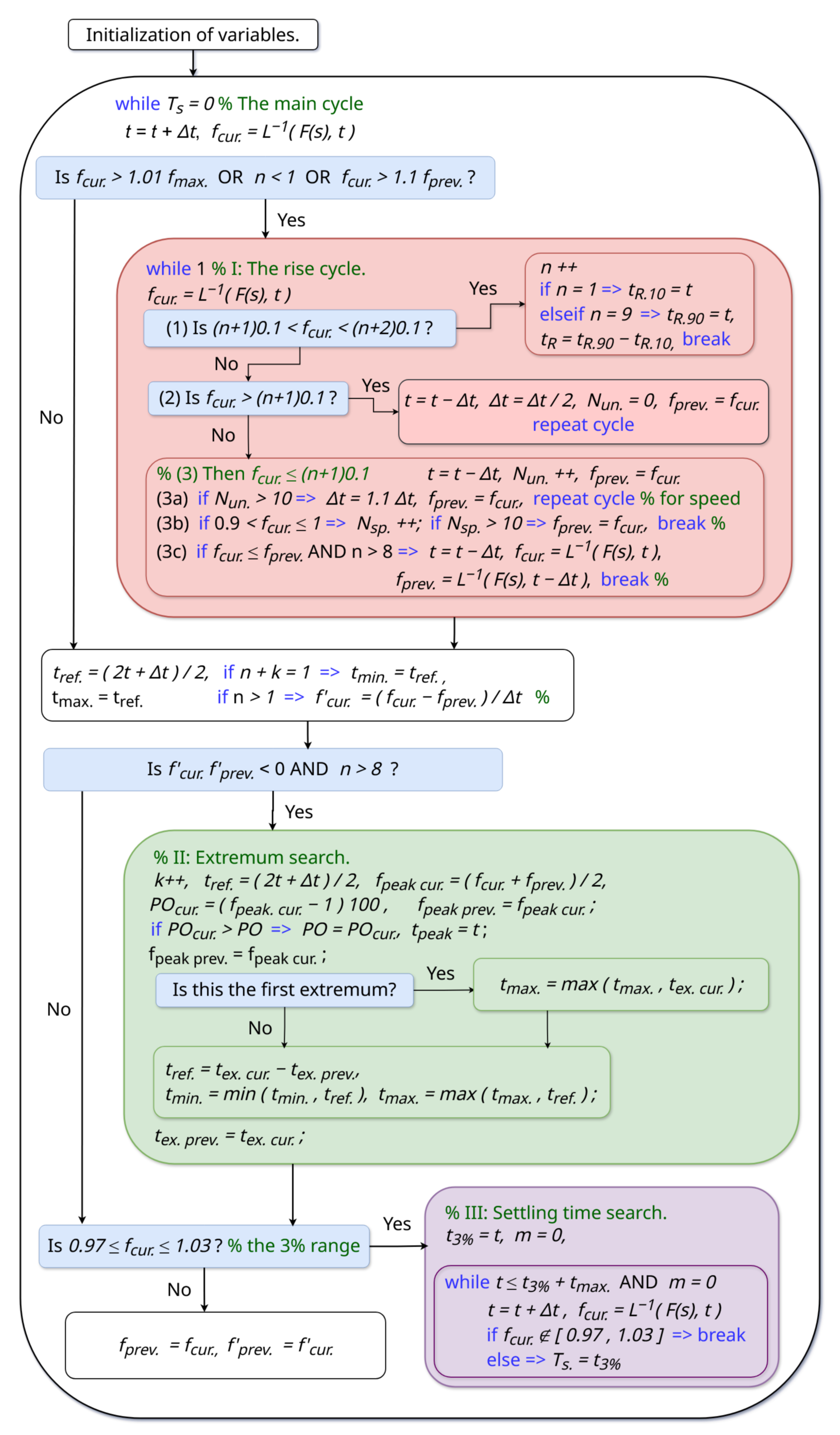
3. The Developed Algorithm

Numerical Tests

The standard approach towards the determination of step response characteristics is to have equal time steps and measure the entire response all the way to the settling time. Then, to determine the overshoot, for example, one simply finds a maximum of the array of signal values. The idea behind the developed algorithm is to gain additional computational speed with a variable time step. This can be achieved if we acknowledge the fact that a step response for a stable linear time invariant system

1.

starts with $f\left(t\right)=0;$

2.

reaches a known steady state value (unity, for example);

3.

is a continuous function for $t>0$.

The third item in the fractional-order case needs a further explanation. If a complex function is analytic at all finite points of the complex plane, it is called an entire (or integral) function. If $\alpha$ and $\beta$ are real and positive, the series in (11) and (13) converge for any value function of y and t, so ${\xi }_k(t,y;\alpha ,\beta )$ is an entire function [4,36]. This means that it is infinitely differentiable for any given finite time t and, therefore, continuous.

Here, we construct a special procedure (see Figure 2 for a diagram) for a faster determination of the main step response parameters like percentage overshoot $PO$, rise time $t_R,$ peak time $t_{peak}$, and settling time $T_s$. This method also pays attention to the number of oscillations k. The algorithm accepts a transfer function $F\left(s\right)$ as an input and outputs $PO,T_s,t_R,t_{peak}$ and k. This procedure is an improvement on the one in [37]. First, we introduce the variables and their initial values:

• t—time (in seconds) for modeling a step response within the algorithm; starts from zero.
• $f_{cur.}$—the value of the step response signal at the current time t, $f_{prev.}$—at the previous time step.
• $f_{cur.}^{\prime }$—the value of the step response signal’s derivative at the current time t, $f_{prev.}^{\prime }$—at the previous time step.
• $\Delta t$—time step. This value changes with the algorithm’s progression, depending on the step response curve. The initial value is close to zero so much that one can ignore any signal changes before the first time step $(0,\Delta t),$ for example 1 ms. This value increases rapidly (see case 3b in the rise cycle in Figure 2).
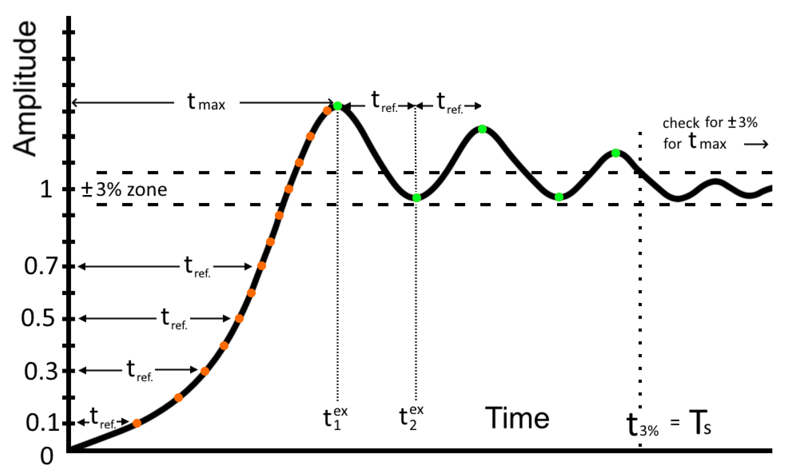
• $t_{ref.}$—the current recorded reference time. This value changes when the signal crosses a decimal value for the first time. It is also compared to the intervals of time between oscillations, if any.
• n—number of decimal values of amplitude the signal has crossed.
• k—number of local extrema.
• $t_{min}$—the minimum of the recorded $t_{ref.}$. The time step $\Delta t$ is calculated based on this parameter. This provides the algorithm with the ability to distinguish possible rapid oscillations.
• $N_{un.}$—the number of undershoots in case 3b.
• $t_{max}$—the largest reference time $t_{ref}.$ This is used as a measure for determining $T_s$.
• $t_{ex.cur.}$—the time of a current detected local extremum, $t_{ex.prev.}$—the time of the previous one.
• $f_{peakcur.}$—the amplitude of a current detected local extremum, $f_{peakprev.}$—same for the previous one.
• $t_{3\%}$—the moment when the signal reaches a $\pm 3\%$ range of the steady state value (1, for example).
• $P{O}_{cur.}$—current recorded value of percentage overshoot. May change depending on the curve.

The initial values for all of the mentioned parameters are zero except for those that were specifically mentioned otherwise. Let us go through the procedures in Figure 2 step by step. The rise cycle is responsible for an ordered recording of time moments when the signal has crossed decimal values for the first time. An efficient way to decide, whether to start it, is to check and see if the current signal value is significantly higher than the maximum or previous values. The check for $n<1$ is there because the first few values of $f_{cur}.$ may be extremely small (maybe even considered negative) due to the way a computer completes calculations. We have noticed this happening more frequently with higher order systems.

The rise cycle consists of three cases. The first one means that $f_{cur.}$ has fell in between the decimal values consequently, so the cycle stops (the orange dots in Figure 3). The second one represents an overshoot of the next decimal value. Time t is shifted one $\Delta t$ back and the time step $\Delta t$ is halved. The third case is an undershoot of the next decimal value and is the most interesting in terms of optimization. Case 3a is a correction of $\Delta t$, which adds significant speed to the calculations. Case 3b accommodates for the no overshoot case—a slow rise between $0.9$ and $1.0$ values. Case 3c accommodates the situation when $f_{cur.}>f_{prev.}$ but the signal later never reaches the next decimal value. Otherwise, an infinite loop may occur in some cases. Also, in order to detect the global extremum later, the time is shifted a step back while the $f_{prev.}$ is shifted two steps back.

After the rise cycle a new procedure is initiated—the extremum search (green dots in Figure 3). Along the way, $t_{ref.},t_{min.}$, and $t_{max.}$ are evaluated. The last one is a measure of how long to continue the check for the signal being in the 3% range of the steady state value. This serves as an independent marker for the input transfer function $F\left(s\right),$ so the user does not have to provide the algorithm with any additional information about the expected signal. If the signal stayed in the 3% range for a duration of $t_{max}$, the algorithm stops as it has reached its final goal.

4. Results and Discussion

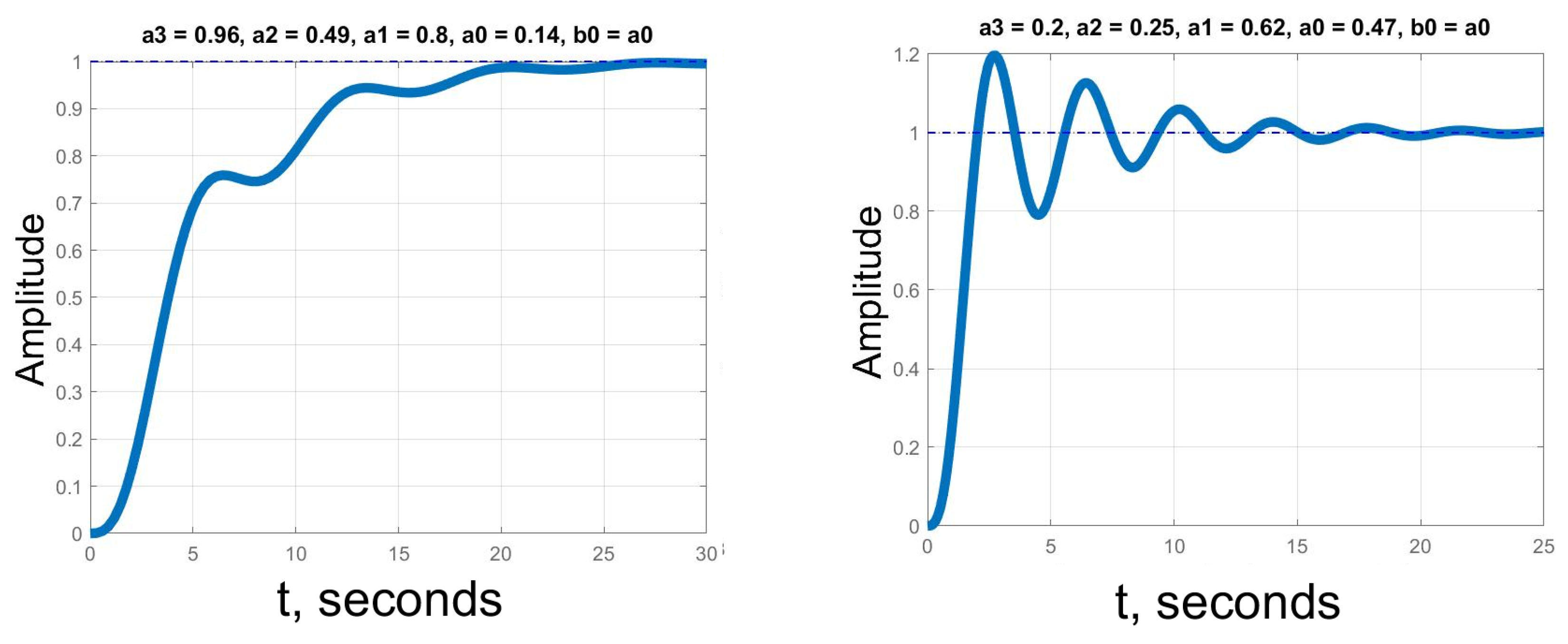
4.1. Numerical Tests

For testing purposes the developed algorithm was coded in Matlab. This provides the ability to measure execution time using the tic toc feature. Secondly, there is the opportunity to compare the computational time with the Matlab’s Control System Toolbox [1] built-in stepinfo function. We have tested transfer functions of linear systems from the second to sixth order:

$$F\left(s\right)={\displaystyle \frac{b_0}{a_n{s}^n+a_{n-1}{s}^{n-1}+\cdots +a_{1}s+a_0}},$$

(14)

where $b_0=a_0$ is to provide for a unity step response. The coefficients were random and uniformly distributed $a_i=\mathtt{rand},a_i\in (0,1).$ The polynomial in the denominator was checked for positive roots. If there was at least one, meaning that the system is unstable, the coefficients were re-calculated. The procedure for testing the efficiency of the developed algorithm was as follows: In order to equalize the starting conditions of both methods, a pause of ten seconds using pause(10) preceded every computation for both methods. Each transfer function was tested ten times, and at each iteration, two computational times were recorded. One time is by Matlab’s stepinfo function $t_{Matlab}$ and the other by the developed algorithm $t_{alg.}.$ The ratios of the mean times of the compared methods $<t_{alg.}>/<t_{Matlab}>$ are presented in the last column of

Table 1. Transfer functions of increasing order with random coefficients. The last row represents the ratio between the mean computational times of the two methods.

$\mathit{F}\left(\mathit{s}\right)$	$\mathit{PO}$	${\mathit{T}}_{\mathit{s}}$	${\mathit{t}}_{\mathit{R}}$	$\frac{<{\mathit{t}}_{\mathit{alg}.}>}{<{\mathit{t}}_{\mathit{Matlab}}>}$
$a_2=0.82, a_1=0.96, a_0=0.01, b_0=a_0$	0	351	205	0.2
$a_2=0.89, a_1=0.39, a_0=0.13, b_0=a_0$	11.7	15.2	4.68	0.61
$a_3=0.96, a_2=0.49, a_1=0.8, a_0=0.14, b_0=a_0$	0	20.4	9.83	0.26
$a_3=0.2, a_2=0.25, a_1=0.62, a_0=0.47, b_0=a_0$	19.5	13.7	1.17	0.27
$a_4=0.35, a_3=0.82, a_2=0.48,$ $a_1=0.98, a_0=0.063, b_0=a_0$	3.26	203	57.6	0.52
$a_4=0.92, a_3=0.27, a_2=0.81,$ $a_1=0.13, a_0=0.11, b_0=a_0$	84.5	50.2	2.24	0.86
$a_5=0.052, a_4=0.22, a_3=0.46, a_2=0.96,$ $a_1=0.79, a_0=0.45, b_0=a_0$	16.1	13.2	1.45	0.57
$a_5=0.026, a_4=0.63, a_3=0.65, a_2=0.6,$ $a_1=0.51, a_0=0.068, b_0=a_0$	9.94	364	9.51	0.82
$a_6=0.16, a_5=0.4, a_4=0.64, a_3=0.7,$ $a_2=0.45, a_1=0.28, a_0=0.067, b_0=a_0$	40.2	205	2.4	0.91
$a_6=0.063, a_5=0.41, a_4=0.89, a_3=0.88,$ $a_2=0.94,a_1=0.34,a_0=0.094,b_0=a_0$	15.3	22.8	3.19	0.73

.

We have mentioned before that acquiring the output characteristics is, in a way, a bottle neck of the optimization problem (1), as seen in Figure 1. In this work we have tried to solve this by creating a faster method for acquiring those characteristics.

First, let us look at second-order systems (Figure 4). Such systems have exact formulas for overshoot $PO$ and peak time $t_{peak}$, as well as explicit formulas for the rise time $t_R$ and settling time $T_s$ approximations. Because of that, second-order systems are commonly used as approximations in engineering. Four types of step response curves of such systems are distinguished based on the location of roots on the complex plain, namely undamped, underdamped, critically damped, and overdamped. Two of them are shown in Figure 4.

Third-order systems already may yield a different behavior. The left curve in Figure 5, while having almost no overshoot, has an oscillatory component. Depending on the modeled process and the scale of these oscillations, one may find a second-order approximation inadequate. The two examples of fourth-order systems we show in Figure 6 differ even more. The right curve exhibits a fractal behavior of sorts—a sequence of damped oscillations. At the same time, the left curve is also representative as follows: as the order of the differential equation increases, one can observe very frequent oscillations with a rather small amplitude. This quality continues to the fifth and sixth order cases (see Figure 7 and Figure 8).

At last, we discuss the computational time difference. This is where the ideas discussed before and highlighted in Figure 1 come to fruition. On average, the developed algorithm outperformed the Matlab’s built-in stepinfo function in 65% of the calculations. Table 1 shows the highlights of the numerical experiments. One can see that the developed algorithm can be up to 4–5 times faster. In a multi-variable optimization task (1), this will considerably reduce the resources needed to find a solution. Also, it may be a significant advantage in a limited computational power environment. This result brings us to a conclusion that the developed algorithm should be adapted to fractional-order dynamical systems.

As for the fractional order case, consider the following transfer functions:

$$T_2={\displaystyle \frac{b_0}{a_2{s}^{{\beta }_2}+a_1{s}^{{\beta }_1}+a_0}},T_1={\displaystyle \frac{b_0}{a_1{s}^{{\beta }_1}+a_0}},$$

where $b_0=a_0$ and ${\beta }_1,{\beta }_2\in \mathbb{R}$ to provide for a unity step response. We have checked both systems for stability and built their step responses using the FOMCON toolbox [22]. As seen in Figure 9, they are pretty similar to the ones in Figure 4 and Figure 5. As long as one has a method for explicit inverse Laplace transformation, it is possible to implement the designed algorithm for fractional-order systems. We are going to address the problem of obtaining such a rule in the next section. If this rule for the inverse Laplace transform is about as fast as the one known for linear integer-order systems, then the benefit in computational speed is going to be similar. For example, in Figure 4, for a no-overshoot curve, there is a decrease in computational time of around 500%. This would speed up tremendously the solution of optimization problem (1) for fractional-order systems. We hope to approach this in more detail in future research. Now, let us discuss an explicit expression for the inverse Laplace transform for a class of linear fractional-order systems.

4.2. An Explicit Formula for the Fractional Order Case

The numerical test results are a motivation for a similar approach in the fractional-order case. One of the main features of the developed algorithm is the assumption that a variable time step $\Delta t$ can benefit the processing speed of a step response. This, however, can be achieved only in the presence of a fast method for the inverse Laplace transform. In the integer case for a transfer function like (3), it is carried out by a partial fraction expansion, which comes down to a sum of exponents. In the fractional-order case, the process is far more complicated and requires additional effort, which we address below.

Consider a more general inhomogeneous fractional-order differential equation with the left part the same as in (9) and

$$\begin{array}{c}{a}_n{D}^{{\beta }_n}y\left(t\right)+a_{n-1}{D}^{{\beta }_{n-1}}y\left(t\right)+\cdots +a_1{D}^{{\beta }_1}y\left(t\right)+a_0{D}^{{\beta }_0}y\left(t\right)\\ =b_0{D}^{{\alpha }_0}u\left(t\right)+b_1{D}^{{\alpha }_1}u\left(t\right)+b_2{D}^{{\alpha }_2}u\left(t\right)+\cdots +b_N{D}^{{\alpha }_N}u\left(t\right),\end{array}$$

(15)

where ${\alpha }_N>{\alpha }_{N-1}>\cdots >{\alpha }_1>{\alpha }_0$ and $b_0,b_1,\dots ,b_N$ are real numbers. Let ${\alpha }_i<{\beta }_n,$$i=1,2,\dots ,N$. A Laplace transformation yields a more general result than the (10) transfer function:

$$F\left(s\right)={\displaystyle \frac{b_N{s}^{{\alpha }_N}+b_{N-1}{s}^{{\alpha }_{N-1}}+\cdots +b_1{s}^{{\alpha }_1}+b_0{s}^{{\alpha }_0}}{a_n{s}^{{\beta }_n}+a_{n-1}{s}^{{\beta }_{n-1}}+\cdots +a_1{s}^{{\beta }_1}+a_0{s}^{{\beta }_0}}},$$

(16)

The inverse Laplace transformation of (16) is shown in [34] to be

$$f\left(t\right)=\sum _{i=1}^N{b}_i{D}^{{\alpha }_i}{g}_n(t,\psi ).$$

(17)

By applying (13) with the differentiation rule (12), we can rewrite (17) as

$$f\left(t\right)=\sum _{i=1}^N{b}_i{g}_n(t,\psi -{\alpha }_i).$$

(18)

For example, let us consider a fractional-order $P{I}^{\lambda }{D}^{\mu }$ controller. The transfer function of this controller is known to be

$$G_c\left(s\right)={\displaystyle \frac{U\left(s\right)}{E\left(s\right)}}=K_P+K_I{s}^{\lambda }+K_D{s}^{\mu },\lambda ,\mu >0,$$

where $U\left(s\right)$ is the controller’s output and $E\left(s\right)$ is the signal error. A system (10) with this controller has a transfer function of

$$G_{closed}\left(s\right)={\displaystyle \frac{K_P{s}^{\lambda }+K_I+K_D{s}^{\mu +\lambda }}{a_n{s}^{{\beta }_n}+a_{n-1}{s}^{{\beta }_{n-1}}+\cdots +a_1{s}^{{\beta }_1}+a_0{s}^{{\beta }_0}+K_P{s}^{\lambda }+K_I+K_D{s}^{\mu +\lambda }}}$$

(19)

In order to acquire an explicit formula for the unit step response of such a system, one must perform several operations. First, we need to rearrange the denominator powers ${\beta }_n,{\beta }_{n-1},{\beta }_{n-2},\dots ,{\beta }_1,{\beta }_0$ with $\lambda ,(\mu +\lambda )$ and 0 (from the $K_I$ addend) in a descending order:

$${\beta }_n,{\beta }_{n-1},{\beta }_{n-2},\dots ,{\beta }_1,{\beta }_0,\lambda ,(\mu +\lambda ), 0\to {\beta }_{n+3}^{\ast },{\beta }_{n+2}^{\ast },{\beta }_{n+1}^{\ast },\dots ,{\beta }_1^{\ast },{\beta }_0^{\ast }.$$

After this, the ordering of the coefficients in the denominator is changed accordingly:

$$a_n,a_{n-1},a_{n-2},\dots ,a_1,a_0,K_P,K_I,K_D\to a_{n+3}^{\ast },a_{n+2}^{\ast },a_{n+1}^{\ast },\dots ,a_1^{\ast },a_0^{\ast }.$$

Now, the highest power in the denominator has an index of $n+3$. This means that the function in (13) must be changed to

$$\begin{array}{c}{g}_{n+3,cont.}^{\ast }(t,{\psi }^{\ast })={\displaystyle \frac{1}{a_{n+3}^{\ast }}}\sum _{m=0}^{\infty }{\displaystyle \frac{{(-1)}^m}{m!}}\sum _{\begin{array}{c}{k}_0+k_1+\cdots +k_{n+1}=m,\\ k_0\ge 0;\dots k_{n+1}\ge 0\end{array}}(m;k_0,k_1,\dots ,k_{n+1})\\ \times \prod _{i=0}^{n+1}{\left({\displaystyle \frac{a_i^{\ast }}{a_{n+3}^{\ast }}}\right)}^{k_i}{\xi }_m(t,-{\displaystyle \frac{a_{n+2}^{\ast }}{a_{n+3}^{\ast }}};{\beta }_{n+3}^{\ast }-{\beta }_{n+2}^{\ast },{\psi }^{\ast }),\end{array}$$

(20)

where ${\psi }^{\ast }={\beta }_{n+3}^{\ast }+{\sum }_{j=0}^{n+1}({\beta }_{n+2}^{\ast }-{\beta }_j^{\ast })k_j.$

There are three addends in the numerator of (19). Using the rule for differentiation (18), we can write the inverse Laplace transform explicitly:

$$f\left(t\right)=(K_P{D}^{\lambda }+K_I+K_D{D}^{\lambda +\mu })g_{n+3,cont.}^{\ast }(t,{\psi }^{\ast })=$$

$$=K_P{g}_{n+3,cont.}^{\ast }(t,{\psi }^{\ast }-\lambda )+K_I{g}_{n+3,cont.}^{\ast }(t,{\psi }^{\ast })+K_D{g}_{n+3,cont.}^{\ast }(t,{\psi }^{\ast }-\lambda -\mu ).$$

To find the unit step response, one needs to integrate this expression with time t. As an integral of order $-1$, in the end, we obtain

$$\begin{array}{c}{y}_{step}\left(t\right)=K_P{g}_{n+3,cont.}^{\ast }(t,{\psi }^{\ast }-\lambda +1)+K_I{g}_{n+3,cont.}^{\ast }(t,{\psi }^{\ast }+1)\\ +K_D{g}_{n+3,cont.}^{\ast }(t,{\psi }^{\ast }-\lambda -\mu +1).\end{array}$$

(21)

Therefore, we have acquired an explicit expression of an output signal $y\left(t\right)$ of a linear fractional-order system with a $P{I}^{\lambda }{D}^{\mu }$ controller in a feedback loop.

As seen in Figure 2, one of the key requirements of the developed algorithm is the calculation of the current signal value based on the inverse Laplace transform $f_{cur.}=L^{-1}(F\left(s\right),t).$ This part distinguishes it from a lot of other methods for processing a step response. For example, Matlab’s lsim function typically provides the user with a sequential array of signal values. This means that, generally, one cannot ask it to output a signal value at a specified moment, only within a sequence. If a process starts with $t=0$ and one would like to know the value of the signal at $t=t_0\ne 0$, those types of programs must first calculate the system’s behavior at all of the previous moments of time. Quite often, the time steps are equally spaced, either automatically or specified by the user. Matlab’s step function does use variable step solvers, but only for systems with internal delays [1].

This is why for the acquirement of step response characteristics, employing the $L^{-1}(F\left(s\right),t)$ procedure saves the effort of computing and saving signal values at previous time steps. The developed algorithm is able to choose the time step $\Delta t$ and moments of time t based on the described mechanisms which depend only on the step response curve. We believe this is the reason behind the advantages in the calculation time described in Table 1. Since (21) is an explicit expression of a step response of a linear fractional-order system at any time moment $t,$ the developed method easily applies to this general case.

5. Conclusions

1.

In this work, a new method for determining step response characteristics is proposed. Based on the conception of a variable time step which depends on the step response curve, this task can be formulated as a new deterministic algorithm. A full description of the algorithm is presented along with a block diagram. It is able to efficiently handle both integer- and fractional-order systems. This decreases the time it takes to process output signals when modeling dynamical systems. Therefore, the algorithm reduces computational costs for a class of optimization problems.

2.

Numerical tests in the integer-order case yielded significant improvements in computational time. Matlab’s Control System Toolbox built-in functions were used as reference. With the mean values of the calculation time of the developed algorithm being up to 4–5 times lower, this approach showed a significant improvement. The mentioned advantage remains true for highly oscillating systems of a higher order. Therefore, the developed algorithm is useful for solving optimization problems which rely on step response characteristics.

3.

A general type of inhomogeneous fractional-order ordinary differential equations and its transfer function were considered. Using the inverse Laplace transformation, we obtained an explicit expression for the time-domain signal of a $P{I}^{\lambda }{D}^{\mu }$-controlled fractional-order linear system. This expression combined with the results of numerical tests suggest a generalization of the developed approach for the fractional-order case.

References

1. Matlab’s Control System Toolbox User’s Guide; Mathworks: Natick, MA, USA, 2018.
2. Ortigueira, M.D.; Tenreiro Machado, J.A. What is a fractional derivative? J. Comput. Phys. 2015, 293, 4–13. [Google Scholar] [CrossRef]
3. Sikora, B. Remarks on the Caputo Fractional Derivative. MINUT-Matematyka i Informatyka na Uczelniach Technicznych. 2023, Volume 5, pp. 76–84. Available online: https://minut.polsl.pl/articles/B-23-001.pdf (accessed on 20 October 2024).
4. Miller, K.S.; Ross, B. An Introduction to the Fractional Calculus and Fractional Differential Equations; John Wiley & Sons, Inc.: New York, NY, USA, 1993; pp. 48, 300. [Google Scholar]
5. Kilbas, A.A.; Srivastava, H.M.; Trujillo, J.J. (Eds.) Theory and Applications of Fractional Differential Equations; North-Holland Mathematics Studies; Elsevier: Amsterdam, The Netherlands, 2006; Volume 204. [Google Scholar]
6. Caputo, M. Linear model of dissipation whose Q is almost frequency independent–II. Geophys. J. R. Astr. Soc. 1967, 13, 529–539. [Google Scholar] [CrossRef]
7. Almeida, R.; Bastos, N.R.O.; Monteiro, M.T.T. Modeling some real phenomena by fractional differential equations. Math. Methods Appl. Sci. 2015, 39, 4846–4855. [Google Scholar] [CrossRef]
8. Diethelm, K. The Analysis of Fractional Differential Equations: An Application-Oriented Exposition Using Differential Operators of Caputo Type; Series on Complexity, Nonlinearity and Chaos; Springer: Berlin/Heidelberg, Germany, 2010. [Google Scholar]
9. Diethelm, K.; Ford, N.J.; Freed, A.D.; Luchko, Y. Algorithms for the fractional calculus: A selection of numerical methods. Comput. Methods Appl. Mech. Eng. 2005, 194, 743–773. [Google Scholar] [CrossRef]
10. Nise, N.S. Control Systems Engineering; John Wiley and Sons: Hoboken, NJ, USA, 2019. [Google Scholar]
11. William, R.L., II; Lawrence, D.A. Linear State-Space Control Systems, 2nd ed.; John Wiley & Sons: Hoboken, NJ, USA, 2007. [Google Scholar]
12. Tavazoei, M.S. Overshoot in the step response of fractional-order control systems. J. Process. Control. 2012, 22, 90–94. [Google Scholar] [CrossRef]
13. Yuce, A.; Tan, N. Inverse Laplace Transforms of the Fractional Order Transfer Functions. In Proceedings of the 11th International Conference on Electrical and Electronics Engineering (ELECO), Bursa, Turkey, 28–30 November 2019. [Google Scholar] [CrossRef]
14. Yoneda, R.; Moriguchi, Y.; Kuroda, M.; Kawaguchi, N. Servo Control of a Current-Controlled Attractive-Force-Type Magnetic Levitation System Using Fractional-Order LQR Control. Fractal Fract. 2024, 8, 458. [Google Scholar] [CrossRef]
15. Ataslar-Ayyildiz, B.; Karahan, O.; Yilmaz, S. Control and Robust Stabilization at Unstable Equilibrium by Fractional Controller for Magnetic Levitation Systems. Fractal Fract. 2021, 5, 101. [Google Scholar] [CrossRef]
16. Muresan, C.I.; Birs, I. Fractional order control for unstable first order processes with time delays. Fract. Calc. Appl. Anal. 2024, 27, 1709–1733. [Google Scholar] [CrossRef]
17. Swain, S.K.; Sain, D.; Mishra, S.K.; Ghosh, S. Real time implementation of fractional order PID controllers for a magnetic levitation plant. AEU—Int. J. Electron. Commun. 2017, 78, 141–156. [Google Scholar] [CrossRef]
18. Kishore, B.; Rosdiazli, I.; Karsiti, M.N.; Sabo Miya, H.; Vivekananda Rajah, H. Fractional-Order Systems and PID Controllers Using Scilab and Curve Fitting Based Approximation Techniques; Springer: Cham, Switzerland, 2020. [Google Scholar]
19. Muresan, C.I.; Bunescu, I.; Birs, I.; De Keyser, R. A Novel Toolbox for Automatic Design of Fractional Order PI Controllers Based on Automatic System Identification from Step Response Data. Mathematics 2024, 11, 1097. [Google Scholar] [CrossRef]
20. Sabatier, J.; Lanusse, P.; Melchior, P.; Oustaloup, A. Fractional Order Differentiation and Robust Control Design: CRONE, H-Infinity and Motion Control; Springer: Dordrecht, The Netherlands, 2016. [Google Scholar]
21. Xue, D.Y.; Bai, L. Fractional Calculus: Numerical Algorithms and Implementations; Tsinghua University Press: Beijing, China, 2022. [Google Scholar]
22. Tepljakov, A.; Petlenkov, E.; Belikov, J. FOMCON toolbox for modeling, design and implementation of fractional-order control systems. In Applications in Control; De Gruyter: Berlin, Germany, 2019; pp. 211–236. [Google Scholar]
23. Valerio, D.; Costa, J.S.D. Ninteger: A non-integer control toolbox for MATLAB. In Proceedings of the 1st IFAC Workshop on Fractional Differentiation and Its Applications, Bordeaux, France, 19–21 July 2004; pp. 1–7. [Google Scholar]
24. Valerio, D. Ninteger Toolbox for MATLAB. 2008. Available online: https://www.mathworks.com/matlabcentral/fileexchange/8312-ninteger (accessed on 28 October 2024).
25. Duist, L.V.; Gugten, G.V.D.; Toten, D.; Saikumar, N.; HosseinNia, H. FLOreS—Fractional order loop shaping MATLAB toolbox. IFAC Pap. 2018, 51, 545–550. [Google Scholar] [CrossRef]
26. Kochenderfer, M.J.; Wheeler, T.A. Algorithms for Optimization; The MIT Press: Cambridge, MA, USA, 2019. [Google Scholar]
27. Arora, J. Introduction to Optimum Design, 3rd ed.; Academic Press: Waltham, MA, USA, 2012. [Google Scholar]
28. Boyd, S.; Vandenberghe, L. Convex Optimization; 7th print; Cambridge University Press: New York, NY, USA, 2009. [Google Scholar]
29. Arora, R.K. Optimization: Algorithms and Applications; Taylor and Francis/CRC Press: Boca Raton, FL, USA, 2015. [Google Scholar]
30. Wilde, D.J. Principles of Optimal Design; Cambridge University Press: New York, NY, USA, 2017. [Google Scholar]
31. Belegundu, A.D.; Chandrupatla, T.R. Optimization Concepts and Applications in Engineering, 2nd ed.; Cambridge University Press: New York, NY, USA, 2011. [Google Scholar]
32. Doetsch, G. Introduction to the Theory and Application of the Laplace Transformation; Springer: Berlin/Heidelberg, Germany, 1974. [Google Scholar]
33. Rowell, D. Analysis and Design of Feedback Control Systems. Available online: http://web.mit.edu/2.14/www/Handouts/Handouts.html (accessed on 10 October 2024).
34. Podlubny, I. Fractional-order systems and PIλDμ controllers. IEEE Trans. Autom. Control. 1999, 44, 208–214. [Google Scholar] [CrossRef]
35. Agarwal, R.P. A propos d’une note de M. Pierre Humbert. C. R. Seances Acad. Sci. 1953, 236, 2031–2032. [Google Scholar]
36. Cartwright, M.L. Integral Functions; Cambridge University Press: Cambridge, UK, 1962. [Google Scholar]
37. Reznichenko, I.; Podržaj, P. Design Methodology for a Magnetic Levitation System Based on a New Multi-Objective Optimization Algorithm. Sensors 2023, 23, 979. [Google Scholar] [CrossRef] [PubMed]
Figure 1. Scheme of the optimization.
Fractalfract 08 00710 g001
Figure 2. A block diagram of the developed algorithm.
Fractalfract 08 00710 g002
Figure 3. The developed algorithm records time of two types of occurrences—crossings of decimal values (the orange dots) and local extrema (the green dots). The minimum and maximum values of the reference time t r e f . are used as independent measures for finding settling time as well as keeping the sampling rate small enough to automatically provide for the Shannon–Nyquist–Kotelnikov theorem [37].
Fractalfract 08 00710 g003
Figure 4. Step responses of second-order systems.
Fractalfract 08 00710 g004
Figure 5. Step responses of third-order systems.
Fractalfract 08 00710 g005
Figure 6. Step responses of fourth-order systems.
Fractalfract 08 00710 g006
Figure 7. Step responses of fifth-order systems.
Fractalfract 08 00710 g007
Figure 8. Step responses of sixth-order systems.
Fractalfract 08 00710 g008
Figure 9. Step responses of two fractional-order linear systems.
Fractalfract 08 00710 g009