Novel Fractional Order Differential and Integral Models for Wind Turbine Power–Velocity Characteristics

Abstract

This work presents an improved modelling approach for wind turbine power curves (WTPCs) using fractional differential equations (FDE). Nine novel FDE-based models are presented for mathematically modelling commercial wind turbine modules’ power–velocity (P-V) characteristics. These models utilize Weibull and Gamma probability density functions to estimate the capacity factor (CF), where accuracy is measured using relative error (RE). Comparative analysis is performed for the WTPC mathematical models with a varying order of differentiation ($\alpha$) from 0.5 to 1.5, utilizing the manufacturer data for 36 wind turbines with capacities ranging from 150 to 3400 kW. The shortcomings of conventional mathematical models in various meteorological scenarios can be overcome by applying the Riemann–Liouville fractional integral instead of the classical integer-order integrals. By altering the sequence of differentiation and comparing accuracy, the suggested model uses fractional derivatives to increase flexibility. By contrasting the model output with actual data obtained from the wind turbine datasheet and the historical data of a specific location, the models are validated. Their accuracy is assessed using the correlation coefficient (R) and the Mean Absolute Percentage Error (MAPE). The results demonstrate that the exponential model at $\alpha =0.9$ gives the best accuracy of WTPCs, while the original linear model was the least accurate.

1. Introduction

A sustainable future depends on wind energy, which offers a clean, abundant, renewable energy source that lowers greenhouse gas emissions and lessens our reliance on fossil fuels. Air wind speed at certain locations is the main factor influencing the amount of electrical active power generated by wind turbine generators, the wind turbine generator’s tower height, and the power curve’s characterization of the turbine’s power response to variations in wind speed [1,2,3]. The manufacturers of wind turbines use field data of wind speed to capture the power produced by the turbine at each wind speed [4]. Power curves for wind turbine generators vary; even turbines with identical ratings may produce power at various wind speeds. The crucial characteristic is the rated power, cut-in, rated, and cut-out speeds of a wind turbine, as shown in Figure 1 [5]. The turbine begins to produce electricity at cut-in speed. The turbine generates electricity that meets the relevant output at rated speed. The turbine stops producing power at cut-out speed.

Regarding power curve modelling for wind turbines, several studies have been conducted. The authors in [6] provided a comparison of different wind turbine power curve models with respect to thirty-two commercial wind turbines, with ratings ranging between 330 and 7580 kW. The evaluated performance of the selected models for power curve modelling using statistical indicators such as correlation coefficient (R), the Mean Absolute Percentage Error (MAPE), and Relative Error (RE) is used to evaluate the performance of capacity factor (CF) model by comparing 12-month wind speed data at the Misrata location, located in northern Libya, with the Weibull and Gamma distributions during the whole year. Their results indicated that the general model gave the best accuracy for power curve modelling, the approximated power coefficient-based model was the least accurate when it comes to capacity factor estimation, and the most accurate model was the power-coefficient-based model, which was developed based on Weibull and gamma distributions, while the polynomial model was the least accurate. The four models are as follows: exponential, cubic, polynomial, and approximated cubic. These are most frequently used to represent the nonlinear part of a power curve between cut-in and rated speed and were contrasted by the results in [7]. Utilizing data from manufacturer power curves from around 200 turbines with 225–7500 kW of capacity, they assessed the model’s accuracy using the coefficient of determination (R²) as a statistical indicator. According to their findings, the cubic and exponential approximations result in reduced energy estimation errors and higher R², which makes this methodology appropriate given its simplicity. As a result of the polynomial model’s highly sensitive response to the manufacturer’s data, on the other hand, it produces the worst results.

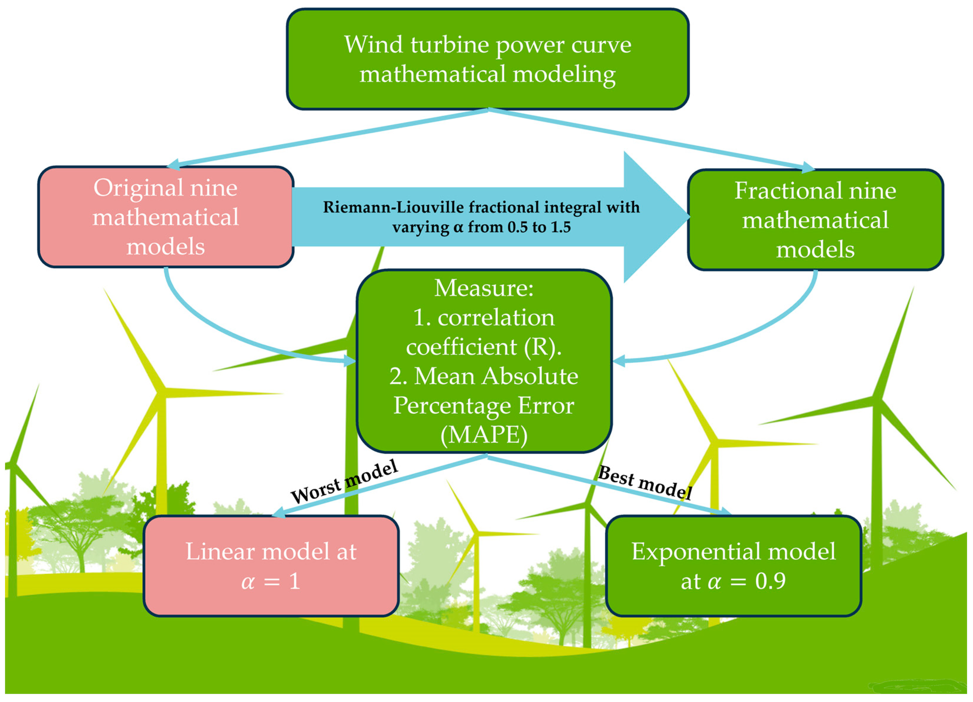
Power curve modelling accurately gives the relationship between wind speed and power output, which is essential for wind turbines. Optimizing turbine performance, forecasting energy production, planning wind farms, and carrying out feasibility studies depend on accurate WTPC modelling. Precise power curve models facilitate the optimal penetration of wind energy into the electrical grid, boosting the dependability of wind power projections and supporting the economical operation and upkeep of wind turbines, all of which ultimately improve wind energy initiatives’ comprehensive efficacy and durability [8].

The modelling of the WTPC is essential to account for these issues. 1. Evaluation of the possibilities for wind power since the wind turbine’s power curve can be utilized for evaluating wind power. It illustrates how wind speed and turbine output power are related to each other. Power curves are provided by manufacturers in tabular or graphical form. However, a mathematical model that precisely calculates the output power from the turbine at any wind speed is necessary for addressing several wind energy system issues, including determining the wind energy potential [9]. 2. Estimation of capacity factor (CF): the capacity factor of the wind turbine can be defined as the ratio of a wind turbine’s actual power output over time to the energy it could have produced, regardless of its location. A wind turbine’s efficiency is reflected in its capacity factor, which shows how well the machine can use the wind’s energy. A wind turbine’s capacity factor is estimated using its power curve. The turbine will be more suitable for the site as the capacity factor value increases. As the capacity factor increases, the wind turbine utilizes more energy from the wind [10]. 3. Wind turbine selection: the power curve can be used to determine if a certain wind turbine is suitable for this site or not according to the output power produced at each wind speed [11]. A graphical abstract of the research can be illustrated in Figure 2.

The flexibility needed to effectively describe complicated meteorological dynamics is frequently limited by integer-order differentiation in standard WTPC models, particularly in areas with changeable wind conditions. The complicated dynamics of wind power generation across various turbine configurations and weather patterns may be overlooked by traditional models based on classical derivatives, which may oversimplify real-world situations. To improve the representation of P-V curves and better match real-world data, fractional generalization aims to address the drawbacks of conventional WTPC models. To maximize wind energy output and guarantee the accuracy of turbine performance evaluations under various circumstances, this improved modelling capability is essential. By introducing FDE, fractional calculus makes it possible to represent the underlying system dynamics more precisely. Memory effects and non-local behaviour, which are frequently seen in wind turbine systems but are not well captured by integer-order models, can be considered by these models by utilizing the fractional derivative. By changing the α from 0.5 to 1.5, these models can be more flexible to accommodate varied turbine capacity and site-specific wind conditions, which improves the accuracy of turbine performance predictions.

The main contributions of the paper can be summarized as follows:

•

We present nine novel fractional order differential and integral mathematical models, tested on various wind turbines across a wide range of ratings to validate the modelling of different 36 WTPCs.

•

We solve FDE using an analytical form for the Riemann–Liouville fractional integral—which will be explained later in Section 4—that is implemented on the model.

•

We study the effect of changing the differentiation order ($\mathit{\alpha }$) for nine mathematical models on the accuracy of WTPC modelling and CF.

•

We utilize a decision-making technique, namely the analytical hierarchy process (AHP), to determine the best model for both WTPCs and CF and the order in which differentiation occurs.

The paper is organized as follows. In Section 3, the system description is discussed in detail. Section 4 focuses on wind turbine power curve mathematical modelling. In Section 5, the results and discussion are presented and analysed. Section 6 provides concluding remarks and summarizes the main findings of this study.

2. Preliminaries

Fractional-order differential operators have received much attention in physics, science, and engineering [12]. More modelling flexibility for dynamic systems and real-world processes is provided by fractional derivatives [13]. These introductions provide the lemmas, insights, and theories required to handle fractional derivatives to address fundamental mathematical concepts. The fractional operators are natural generalizations of the classical integer-order operators that enable modelling extra properties such as the memory and past effects. This allows applications to be extended and opens the door for implying new dimensions.

There are many definitions in the literature for fractional integrals and differentiation operators. In [14], a review, many fractional operators are introduced and classified. Many new fractional operators are still under development, and trials have been undertaken to unify the operators, but still no clear unified operator has been developed [15].

In the current work, we choose the well-known Riemann–Lioiville fractional derivative and integral definitions.

Definition 1

(Riemann–Liouville fractional integral [16]). For a function  $f\left(t\right)$ that is defined, integrable and  $\in L^p[a,b]$, the Riemann–Liouville fractional integral of order  $\alpha >0$ is given by: 

$${(I}_a^{\alpha }f)\left(t\right)={\displaystyle \frac{1}{\Gamma \left(\alpha \right)}}{\int }_a^t{\displaystyle \frac{f\left(\tau \right)}{{\left(t-\tau \right)}^{1-\alpha }}}d\tau ,$$

(1)

 where  $\alpha$ is the order of integration,  $a$ is the lower limit of integral, and  $\Gamma (.)$ is the gamma function defined as: 

$$\Gamma \left(\tau \right)={\int }_0^{\mathrm{\infty }}{x}^{\Gamma -1}{e}^{-x}dx.$$

(2)

The fractional integral operator  ${\mathit{I}}_{\mathit{a}}^{\mathit{\alpha }}$ is linear, continuous and bounded from  ${\mathit{L}}^{\mathit{p}}[\mathit{a},\mathit{b}]$ to itself [17] with the property  ${\displaystyle \underset{\mathit{\alpha }\to 0}{\mathit{lim}}}{‖{(\mathit{I}}_{\mathit{a}}^{\mathit{\alpha }}\mathit{f})\left(\mathit{t}\right)-\mathit{f}(\mathit{t})‖}_{\mathit{p}}=0;\mathit{p}\le 1,\mathit{\alpha }\ge 0$.

A first-order stable numerical approximation of the fractional integral in Equation (1) can be performed using the Grunwald–Letnikov (GL) technique [18]:

$$({\mathit{I}}_{\mathit{a}}^{\mathit{\alpha }}\mathit{f})(\mathrm{t})={\displaystyle \underset{h\to 0}{\lim }}{\displaystyle \frac{1}{h^{\alpha }}}{\sum }_{j=0}^{{\displaystyle \frac{t-a}{h}}} {\displaystyle \frac{\Gamma \left(1-\alpha \right){\left(-1\right)}^j}{\Gamma \left(1+j\right)\Gamma \left(1-\alpha -j\right)}}f\left(t-jh\right) .$$

(3)

Definition 2

(Riemann–Liouville fractional derivative [19]). For a function  $\mathit{f}\left(\mathit{t}\right)$ that is differentiable, the Riemann–Liouville fractional derivative of order α of a function  $\mathit{f}\left(\mathit{t}\right)$ is defined as follows:

$$D_t^{\alpha }\left(f\left(t\right)\right)={\displaystyle \frac{1}{\Gamma (n-\alpha )}}{\displaystyle \frac{d^n}{d{t}^n}}{\int }_a^t{\displaystyle \frac{f\left(\tau \right)}{{\left(t-\tau \right)}^{\alpha -n+1}}}d\tau ,$$

(4)

 where  $n=⌈\alpha ⌉$ is the smallest integer greater than or equal to  $\alpha$. The numerical approximation of Equation (4) can be evaluated with GL definition in Equation (3) after replacing  $\alpha$ with  $-\alpha$.

The fractional derivative can be considered as nth-order differentiation of the fractional integral of order  $n-\alpha$  i.e.,  ${{D_t^{\alpha }\left(f\left(t\right)\right)=D}_t^n(I}_a^{n-\alpha }f)\left(t\right)$. Also, we can verify that  $D_t^{\alpha }\left({(I}_a^{n-\alpha }f\left)\right(t)\right)=f\left(t\right)$ and  ${(I}_a^{\alpha }\left({(I}_a^{\beta }f\left)\right(t)\right)={(I}_a^{\alpha +\beta }f\left)\right(t)$. Another well-known definition for the fractional derivative is the Caputo definition, which can be written as  ${D_t^{\alpha }\left(f\left(t\right)\right)=(I}_a^{n-\alpha }\left(D_t^{n}f\left(t\right)\right)$ [20].

3. System Description

This section consists of three subsections: the first one will introduce the various models of wind speed, the second one will introduce the output power produced from the wind turbine curve and the capacity factor, and the third one will introduce the data required to collect and the region selected for the study.

3.1. Wind Speed Modelling

In statistics, it is essential to determine the mean ($v_{mean}$) and standard deviation (${\sigma }_{vel}$) of any given wind speed data; these can be obtained using [21,22] as follows:

$$v_{mean}={\displaystyle \frac{1}{n}}{\displaystyle \sum _{i=1}^n}{v}_i ,$$

(5)

$${\sigma }_{vel}=\sqrt{{\displaystyle \frac{1}{n-1}}{\displaystyle \sum _{i=1}^n}{\left(v_i-v_{mean}\right)}^2} .$$

(6)

where $v_i$ is the $i^{th}$ speed of wind, and the total number of wind speed data points that the manufacturer has made available is called $n$.

The wind speed is stochastic, so the probability density function (PDF) must be used to assess wind speed behaviour. Because of the cubic relationship between wind speed and wind turbine output power, which means that even a slight fluctuation in wind speed can result in a considerable change in power, the distribution utilized to characterize wind speed impacts the assessment of wind energy potential. For this reason, the selected distribution must be chosen precisely to have accurate results. The Weibull and gamma distributions are the most commonly used distributions to present wind speed data [23,24]. Because of this, the Weibull and gamma distributions will be used in this study’s subsequent computations.

• Weibull distribution

The probability density function $f\left(v\right)$ of the Weibull distribution is given by [25,26,27]:

$$f\left(v\right)=\left({\displaystyle \frac{k}{c}}\right){\left({\displaystyle \frac{v}{c}}\right)}^{k-1}{e}^{-{\left({\displaystyle \frac{v}{c}}\right)}^k},$$

(7)

where $k$ and $c$ represent the Weibull distribution’s dimensionless form and scale in m/s, respectively.

The common methods to evaluate the Weibull parameters k and c are given by the following [26]:

• Graphical method.
• Standard deviation method.
• Moment method.
• Maximum likelihood method.
• Energy pattern factor method.

The standard deviation method is used for its ease of application and high accuracy, according to [26]. The parameters $k$ and $c$ can be evaluated from the mean and standard deviation of wind data. Consider the expressions for the mean and standard deviation for wind speed given in Equations (5) and (6); from these, and according to [26], the following equations can be obtained:

$${\left({\displaystyle \frac{{\sigma }_{vel}}{v_{mean}}}\right)}^2={\displaystyle \frac{\Gamma \left(1+\frac{2}{k}\right)}{{\Gamma }^2\left(1+\frac{1}{k}\right)}}-1.$$

(8)

Once Equation (8) is solved numerically to obtain the value of $k$, $c$ can be given by:

$$c={\displaystyle \frac{v_{mean}}{\Gamma \left(1+\frac{1}{k}\right)}}.$$

(9)

The Weibull cumulative distribution function (CDF), $F\left(v\right)$, is given by [25,26,27]:

$$F\left(v\right)=1-e^{-{\left({\displaystyle \frac{v}{c}}\right)}^k}.$$

(10)

The $v_{mean}$ and ${\sigma }_{vel}$ of the Weibull distribution are given as follows:

$$v_{mean}=c\Gamma \left(1+{\displaystyle \frac{1}{k}}\right),$$

(11)

$${\sigma }_{vel}=c\sqrt{\Gamma \left(1+{\displaystyle \frac{2}{k}}\right)-{\Gamma }^2\left(1+{\displaystyle \frac{1}{k}}\right)}.$$

(12)

2.

Gamma distribution

The gamma PDF $f\left(v\right)$ is given by [28,29]:

$$f\left(v\right)={\displaystyle \frac{v^{\alpha -1}}{\Gamma \left(\alpha \right){\beta }^{\alpha }}}{e}^{-{\displaystyle \frac{v}{\beta }}},$$

(13)

where $\alpha$ and $\beta$ are the dimensionless shape and scale in m/s, and v is the wind speed in m/s, given by [26,27]:

$$\alpha ={\displaystyle \frac{v_{mean}^2}{{\sigma }_{vel}^2}},$$

(14)

$$\beta ={\displaystyle \frac{{\sigma }_{vel}^2}{v_{mean}}}.$$

(15)

3.2. Turbine Power Output and Capacity Factor

The power output $P\left(v\right)$ generated by a wind turbine can be classified into four regions according to $v$, as shown in Figure 1, given by [3,4]:

$$P\left(v\right)=\left\{\begin{array}{ccc}0\hfill & ,& v<v_{ci}\\ P_m\left(v\right)\hfill & ,& v_{ci}\le v<v_r\\ P_r\hfill & ,& v_r\le v<v_{co}\\ 0\hfill & ,& v\ge v_{co}\end{array}\right.$$

(16)

where $v_{ci},v_r$, $v_{co}$ are the cut-in, rated, and cut-out wind speeds, respectively, $P_r$ is the rated wind turbine output power in Watt, and $P_m\left(v\right)$ is the output power. The total output energy $E_{out}$ in Watt-hour (Whr) produced by a wind turbine over a certain period $T$ can be calculated given the following formula [3,4]:

$$E_{out}=T{\int }_{v_{ci}}^{v_{co}}P\left(v\right)f\left(v\right)dv,$$

$$E_{out}=T\left[{\int }_{v_{ci}}^{v_r}{P}_m\left(v\right)f\left(v\right)dv+P_r{\int }_{v_r}^{v_{co}}f\left(v\right)dv\right].$$

(17)

The method by which the turbine utilizes the energy from the wind is indicated by the capacity factor (CF). By using PDF used to model wind speed, the CF can be estimated, given by [3,4,21,25]:

$${CF}_{pdf}={\displaystyle \frac{E_{out}}{P_r\ast T}}.$$

(18)

Also, based on the recorded time-series wind speeds, CF can be calculated using the following [30]:

$${CF}_{ts}={\displaystyle \frac{AEO}{P_r\ast T}},$$

(19)

where $AEO$ is the total annual energy output produced by a wind turbine and can be calculated using actual data from the site at which the wind turbine was installed, given as [30]:

$$AEO={\displaystyle \sum _{i=1}^n}{MPC}_i\ast H_i,$$

(20)

where MPCi is the power curve value provided by the manufacturer in watts corresponding to wind speed bin $i$ and obtained from the site’s historical data, H_i is the total hours during which the wind speed was recorded at bin $i$, and there are $n$ bins in total; this value is typically taken to be 25.

3.3. Data Collection and Case Study Region

The Zafarana site provided the wind speed measurements used in the present study, which is a 545 MW onshore wind power project in Egypt, according to the Egyptian New and Renewable Energy Authority (NREA) [31]. It is considered the largest wind power energy project in Egypt. The wind speed was recorded, and the considered data were from the year 2023. The performance of the suggested fractional models was assessed using the data in order to calculate the capacity factor.

4. Wind Turbine Power Curve Mathematical Modelling

The objective of this research was to compare the performance of nine mathematical fractional models at different orders of differentiation ($\alpha$) ranging $0.5–1.5$ with a step size of 0.1 of WTPCs, with the original mathematical models stated in study [6], using a different wind turbine dataset and finding out for each model which $\mathsf{\alpha }$ for each model gives the best performance in depicting the power curve’s behaviour given by manufacturers. The range of α from 0.5 to 1.5 was selected to capture both sub-integer and super-integer behaviour around the classical integer order 1, allowing for a more flexible and comprehensive exploration of model performance. After that, we ranked the models using a decision-making technique called analytical hierarchy process (AHP) to determine the overall ranks for the models according to statistical criteria. The proposed models described in this section are as follows.

4.1. Wind Turbine Power–Velocity Curve Mathematical Models

Some fractional integrals using the Riemann–Liouville fractional integral definition were used in mathematical modelling; these can be summarized as follows:

$$I_a^{\alpha }{\left(x-a\right)}^{\beta }={\displaystyle \frac{\Gamma \left(\beta +1\right)}{\Gamma \left(\alpha +\beta +1\right)}}{\left(x-a\right)}^{\alpha +\beta },$$

(21)

where $a\in \mathbb{C},\alpha >0,Re\left(\beta \right)>-1.$

$$I_a^{\alpha }\left(c\right)={\displaystyle \frac{\mathrm{c}}{\Gamma \left(\alpha +1\right)}}{\left(x-a\right)}^{\alpha },$$

(22)

where $c$ is an arbitrary constant, $a\in \mathbb{C},\alpha \in \mathbb{R}$.

4.1.1. Linear Model

In the linear model, the second part of the power curve $[v_{ci},v_r)$, the output power and wind speed have a linear relationship. The output power in this region is given by [32]:

$$P_m\left(v\right)=P_r\left({\displaystyle \frac{v-v_{ci}}{v_r-v_{ci}}}\right).$$

(23)

which means the power differential with respect to velocity is constant, i.e.,

$${\displaystyle \frac{d{P}_m\left(v\right)}{dv}}={\displaystyle \frac{P_r}{v_r-v_{ci}}}.$$

A modification is performed to convert the model to a fractional model by replacing the integer first ordinary derivative with $\alpha$ fractional derivative and then using Riemann–Liouville fractional integration of order $\alpha$:

$${\mathit{P}}_{\mathit{m}}\left(\mathit{v}\right)={\mathit{I}}_{{\mathit{v}}_{\mathit{c}\mathit{i}}}^{\mathit{\alpha }}\left({\displaystyle \frac{{\mathit{P}}_{\mathit{r}}}{{\mathit{v}}_{\mathit{r}}-{\mathit{v}}_{\mathit{c}\mathit{i}}}}\right).$$

(24)

The fractional integral of a constant is applied to obtain:

$$P_m\left(v\right)={\displaystyle \frac{P_r{\left(v-v_{ci}\right)}^{\alpha }}{\Gamma \left(\alpha +1\right)\left(v_r-v_{ci}\right)}}.$$

(25)

We can note that Equation (25) reduces to Equation (23) for $\alpha =1$.

4.1.2. Quadratic MODEL

In this model, the second part of the power curve $[v_{ci},v_r)$ has a quadratic relationship. The output power in this region is given by [32,33,34]:

$$P_m\left(v\right)=P_r\left({\displaystyle \frac{v^2-v_{ci}^2}{v_r^2-v_{ci}^2}}\right).$$

(26)

This means that the power derivative with respect to $v$ can be obtained as follows:

$${\displaystyle \frac{d{P}_m\left(v\right)}{dv}}={\displaystyle \frac{{2P}_{r}v}{v_r^2-v_{ci}^2}}.$$

By considering the fractional derivative of order $\alpha$ in place of the integer first derivative and integrate, we obtain:

$${\mathit{P}}_{\mathit{m}}\left(\mathit{v}\right)={\mathit{I}}_{{\mathit{v}}_{\mathit{c}\mathit{i}}}^{\mathit{\alpha }}\left({\displaystyle \frac{{\mathbf{2}\mathit{P}}_{\mathit{r}}\mathit{v}}{{\mathit{v}}_{\mathit{r}}^{\mathbf{2}}-{\mathit{v}}_{\mathit{c}\mathit{i}}^{\mathbf{2}}}}\right),$$

which can be re-written as:

$$P_m\left(v\right)=I_{v_{ci}}^{\alpha }\left({\displaystyle \frac{{2P}_r\left(v-v_{ci})\right)}{v_r^2-v_{ci}^2}}\right)+I_{v_{ci}}^{\alpha }\left({\displaystyle \frac{{2P}_r{v}_{ci}}{v_r^2-v_{ci}^2}}\right).$$

The first integral can be expressed using Equation (21) to obtain:

$${\mathit{I}}_{{\mathit{v}}_{\mathit{c}\mathit{i}}}^{\mathit{\alpha }}\left({\displaystyle \frac{{\mathbf{2}\mathit{P}}_{\mathit{r}}\left(\mathit{v}-{\mathit{v}}_{\mathit{c}\mathit{i}})\right)}{{\mathit{v}}_{\mathit{r}}^{\mathbf{2}}-{\mathit{v}}_{\mathit{c}\mathit{i}}^{\mathbf{2}}}}\right)={\displaystyle \frac{\mathbf{2}{\mathit{P}}_{\mathit{r}}}{{(\mathit{v}}_{\mathit{r}}^{\mathbf{2}}-{\mathit{v}}_{\mathit{c}\mathit{i}}^{\mathbf{2}})}}.{\displaystyle \frac{\mathbf{1}}{\mathbf{\Gamma }\left(\mathit{\alpha }+\mathbf{2}\right)}}.{\left(\mathit{v}-{\mathit{v}}_{\mathit{c}\mathit{i}}\right)}^{\mathit{\alpha }+\mathbf{1}}.$$

(27)

The second integral can be expressed using Equation (22) to obtain:

$${\mathit{I}}_{{\mathit{v}}_{\mathit{c}\mathit{i}}}^{\mathit{\alpha }}\left({\displaystyle \frac{{\mathbf{2}\mathit{P}}_{\mathit{r}}{\mathit{v}}_{\mathit{c}\mathit{i}}}{{\mathit{v}}_{\mathit{r}}^{\mathbf{2}}-{\mathit{v}}_{\mathit{c}\mathit{i}}^{\mathbf{2}}}}\right)={\displaystyle \frac{\mathbf{2}{\mathit{P}}_{\mathit{r}}{\mathit{v}}_{\mathit{c}\mathit{i}}}{{(\mathit{v}}_{\mathit{r}}^{\mathbf{2}}-{\mathit{v}}_{\mathit{c}\mathit{i}}^{\mathbf{2}})}}.{\displaystyle \frac{\mathbf{1}}{\mathbf{\Gamma }\left(\mathit{\alpha }+\mathbf{1}\right)}}.{\left(\mathit{v}-{\mathit{v}}_{\mathit{c}\mathit{i}}\right)}^{\mathit{\alpha }}.$$

(28)

Adding Equations (27) and (28) results in a quadratic fractional model as follows:

$${\mathit{P}}_{\mathit{m}}\left(\mathit{v}\right)={\displaystyle \frac{2{\mathit{P}}_{\mathit{r}}{\left(\mathit{v}-{\mathit{v}}_{\mathit{c}\mathit{i}}\right)}^{\mathit{\alpha }}}{\mathbf{\Gamma }\left(\mathit{\alpha }+\mathbf{1}\right){(\mathit{v}}_{\mathit{r}}^{\mathbf{2}}-{\mathit{v}}_{\mathit{c}\mathit{i}}^{\mathbf{2}})}}\left[{\displaystyle \frac{(\mathit{v}-{\mathit{v}}_{\mathit{c}\mathit{i}})}{\left(\mathit{\alpha }+\mathbf{1}\right)}}+{\mathit{v}}_{\mathit{c}\mathit{i}}\right].$$

(29)

We can note that the fractional model in Equation (29) will reduce to Equation (26) for $\alpha =1$.

4.1.3. Cubic Type-I Model

The power output and wind speed relationship in the cubic type-I model is cubic without taking v_ci and v_r into consideration in the second region of the power curve $[v_{ci},v_r)$. The output power in this region is given by [7]:

$$P_m\left(v\right)=P_r\left({\displaystyle \frac{v^3}{v_r^3}}\right).$$

(30)

This means that the power derivative with respect to $v$ can be obtained as follows:

$${\displaystyle \frac{d{P}_m\left(v\right)}{dv}}={\displaystyle \frac{{3P}_r{v}^2}{v_r^3}}.$$

By considering the fractional derivative of order $\alpha$ in place of the integer first derivative and integrate, we obtain:

$${\mathit{P}}_{\mathit{m}}\left(\mathit{v}\right)={\mathit{I}}_{{\mathit{v}}_{\mathit{c}\mathit{i}}}^{\mathit{\alpha }}\left({\displaystyle \frac{{\mathbf{3}\mathit{P}}_{\mathit{r}}{\mathit{v}}^{\mathbf{2}}}{{\mathit{v}}_{\mathit{r}}^{\mathbf{3}}}}\right),$$

which can be re-written as:

$$P_m\left(v\right)=I_{v_{ci}}^{\alpha }\left({\displaystyle \frac{{3P}_r{\left(v-v_{ci}\right)}^2}{v_r^3}}\right)+I_{v_{ci}}^{\alpha }\left({\displaystyle \frac{{6P}_r{v}_{ci}(v-v_{ci})}{v_r^3}}\right)+I_{v_{ci}}^{\alpha }\left({\displaystyle \frac{{3P}_r{v}_{ci}^2}{v_r^3}}\right).$$

The first integral can be expressed using Equation (21) to obtain:

$${\mathit{I}}_{{\mathit{v}}_{\mathit{c}\mathit{i}}}^{\mathit{\alpha }}\left({\displaystyle \frac{{\mathbf{3}\mathit{P}}_{\mathit{r}}{\left(\mathit{v}-{\mathit{v}}_{\mathit{c}\mathit{i}}\right)}^{\mathbf{2}}}{{\mathit{v}}_{\mathit{r}}^{\mathbf{3}}}}\right)={\displaystyle \frac{\mathbf{3}{\mathit{P}}_{\mathit{r}}}{{\mathit{v}}_{\mathit{r}}^{\mathbf{3}}}}.{\displaystyle \frac{\mathbf{\Gamma }\left(\mathbf{3}\right)}{\mathbf{\Gamma }\left(\mathit{\alpha }+\mathbf{3}\right)}}.{\left(\mathit{v}-{\mathit{v}}_{\mathit{c}\mathit{i}}\right)}^{\mathit{\alpha }+\mathbf{2}}.$$

(31)

The second integral can be expressed using Equation (21) to obtain:

$${\mathit{I}}_{{\mathit{v}}_{\mathit{c}\mathit{i}}}^{\mathit{\alpha }}\left({\displaystyle \frac{{\mathbf{6}\mathit{P}}_{\mathit{r}}{\mathit{v}}_{\mathit{c}\mathit{i}}(\mathit{v}-{\mathit{v}}_{\mathit{c}\mathit{i}})}{{\mathit{v}}_{\mathit{r}}^{\mathbf{3}}}}\right)={\displaystyle \frac{\mathbf{6}{\mathit{P}}_{\mathit{r}}{\mathit{v}}_{\mathit{c}\mathit{i}}}{{\mathit{v}}_{\mathit{r}}^{\mathbf{3}}}}.{\displaystyle \frac{\mathbf{\Gamma }\left(\mathbf{2}\right)}{\mathbf{\Gamma }\left(\mathit{\alpha }+\mathbf{2}\right)}}.{\left(\mathit{v}-{\mathit{v}}_{\mathit{c}\mathit{i}}\right)}^{\mathit{\alpha }+\mathbf{1}}.$$

(32)

For the third integral, it may be expressed using Equation (22) to obtain:

$${\mathit{I}}_{{\mathit{v}}_{\mathit{c}\mathit{i}}}^{\mathit{\alpha }}\left({\displaystyle \frac{{\mathbf{3}\mathit{P}}_{\mathit{r}}{\mathit{v}}_{\mathit{c}\mathit{i}}^{\mathbf{2}}}{{\mathit{v}}_{\mathit{r}}^{\mathbf{3}}}}\right)={\displaystyle \frac{\mathbf{3}{\mathit{P}}_{\mathit{r}}{\mathit{v}}_{\mathit{c}\mathit{i}}^{\mathbf{2}}}{{\mathit{v}}_{\mathit{r}}^{\mathbf{3}}}}.{\displaystyle \frac{\mathbf{1}}{\mathbf{\Gamma }\left(\mathit{\alpha }+\mathbf{1}\right)}}.{\left(\mathit{v}-{\mathit{v}}_{\mathit{c}\mathit{i}}\right)}^{\mathit{\alpha }}.$$

(33)

Adding Equations (31)–(33) results in a cubic type-I fractional model, as follows:

$${\mathit{P}}_{\mathit{m}}\left(\mathit{v}\right)={\displaystyle \frac{\mathbf{3}{\mathit{P}}_{\mathit{r}}{\left(\mathit{v}-{\mathit{v}}_{\mathit{c}\mathit{i}}\right)}^{\mathit{\alpha }}}{{\mathbf{\Gamma }\left(\mathit{\alpha }+\mathbf{1}\right)\mathit{v}}_{\mathit{r}}^{\mathbf{3}}}}\left[{\displaystyle \frac{\mathbf{2}{\left(\mathit{v}-{\mathit{v}}_{\mathit{c}\mathit{i}}\right)}^{\mathbf{2}}}{\left(\mathit{\alpha }+\mathbf{1}\right)\left(\mathit{\alpha }+\mathbf{2}\right)}}+{\displaystyle \frac{\mathbf{2}{\mathit{v}}_{\mathit{c}\mathit{i}}(\mathit{v}-{\mathit{v}}_{\mathit{c}\mathit{i}})}{\left(\mathit{\alpha }+\mathbf{1}\right)}}+{\mathit{v}}_{\mathit{c}\mathit{i}}^{\mathbf{2}}\right].$$

(34)

We can note that the fractional model in Equation (34) will reduce to Equation (30) for $\alpha =1$.

4.1.4. Cubic Type-II Model

The power output and wind speed relationship in the cubic type-II model is cubic by taking v_ci and v_r into consideration in the second region of the power curve $[v_{ci},v_r)$. The output power in this region is given by [35]:

$$P_m\left(v\right)=P_r\left({\displaystyle \frac{v^3-v_{ci}^3}{v_r^3-v_{ci}^3}}\right).$$

(35)

This means that the power derivative with respect to $v$ can be obtained as follows:

$${\displaystyle \frac{d{P}_m\left(v\right)}{dv}}={\displaystyle \frac{{3P}_r{v}^2}{v_r^3-v_{ci}^3}}.$$

By considering the fractional derivative of order $\alpha$ in place of the integer first derivative and integrate, we obtain:

$${\mathit{P}}_{\mathit{m}}\left(\mathit{v}\right)={\mathit{I}}_{{\mathit{v}}_{\mathit{c}\mathit{i}}}^{\mathit{\alpha }}\left({\displaystyle \frac{{\mathbf{3}\mathit{P}}_{\mathit{r}}{\mathit{v}}^{\mathbf{2}}}{{\mathit{v}}_{\mathit{r}}^{\mathbf{3}}-{\mathit{v}}_{\mathit{c}\mathit{i}}^{\mathbf{3}}}}\right),$$

which can be re-written as:

$${\mathit{P}}_{\mathit{m}}\left(\mathit{v}\right)={\mathit{I}}_{{\mathit{v}}_{\mathit{c}\mathit{i}}}^{\mathit{\alpha }}\left({\displaystyle \frac{{\mathbf{3}\mathit{P}}_{\mathit{r}}{\left(\mathit{v}-{\mathit{v}}_{\mathit{c}\mathit{i}}\right)}^{\mathbf{2}}}{{\mathit{v}}_{\mathit{r}}^{\mathbf{3}}-{\mathit{v}}_{\mathit{c}\mathit{i}}^{\mathbf{3}}}}\right)+{\mathit{I}}_{{\mathit{v}}_{\mathit{c}\mathit{i}}}^{\mathit{\alpha }}\left({\displaystyle \frac{{\mathbf{6}\mathit{P}}_{\mathit{r}}{\mathit{v}}_{\mathit{c}\mathit{i}}(\mathit{v}-{\mathit{v}}_{\mathit{c}\mathit{i}})}{{\mathit{v}}_{\mathit{r}}^{\mathbf{3}}-{\mathit{v}}_{\mathit{c}\mathit{i}}^{\mathrm{3}}}}\right)+{\mathit{I}}_{{\mathit{v}}_{\mathit{c}\mathit{i}}}^{\mathit{\alpha }}\left({\displaystyle \frac{{\mathbf{3}\mathit{P}}_{\mathit{r}}{\mathit{v}}_{\mathit{c}\mathit{i}}^{\mathbf{2}}}{{\mathit{v}}_{\mathit{r}}^{\mathbf{3}}-{\mathit{v}}_{\mathit{c}\mathit{i}}^{\mathbf{3}}}}\right).$$

This is the same as in the previous model, with only the constant changed, where the cubic type-II fractional model is given as:

$${\mathit{P}}_{\mathit{m}}\left(\mathit{v}\right)={\displaystyle \frac{\mathbf{3}{\mathit{P}}_{\mathit{r}}{\left(\mathit{v}-{\mathit{v}}_{\mathit{c}\mathit{i}}\right)}^{\mathit{\alpha }}}{{\mathbf{\Gamma }\left(\mathit{\alpha }+\mathbf{1}\right)(\mathit{v}}_{\mathit{r}}^{\mathbf{3}}-{\mathit{v}}_{\mathit{c}\mathit{i}}^{\mathbf{3}})}}\left[{\displaystyle \frac{\mathbf{2}{\left(\mathit{v}-{\mathit{v}}_{\mathit{c}\mathit{i}}\right)}^{\mathbf{2}}}{\left(\mathit{\alpha }+\mathbf{1}\right)\left(\mathit{\alpha }+\mathbf{2}\right)}}+{\displaystyle \frac{\mathbf{2}{\mathit{v}}_{\mathit{c}\mathit{i}}(\mathit{v}-{\mathit{v}}_{\mathit{c}\mathit{i}})}{\left(\mathit{\alpha }+\mathbf{1}\right)}}+{\mathit{v}}_{\mathit{c}\mathit{i}}^{\mathbf{2}}\right].$$

(36)

We can note that the fractional model in Equation (36) will reduce to Equation (35) for $\alpha =1$.

4.1.5. General $m^{th}$ Order Model

The relationship in the general model is in $m^{th}$ order, taking vci and vr into consideration in the second region of the power curve $[v_{ci},v_r)$. The output power in this region is given by [32]:

$$P_m\left(v\right)=P_r\left({\displaystyle \frac{v^m-v_{ci}^m}{v_r^m-v_{ci}^m}}\right).$$

(37)

This means that the power derivative with respect to $v$ can be obtained as follows:

$${\displaystyle \frac{d{P}_m\left(v\right)}{dv}}={\displaystyle \frac{{mP}_r{v}^{m-1}}{v_r^{\mathrm{m}}-v_{ci}^m}},$$

where the output power curve’s order, denoted by m, is assumed to be 2.4 in this research.

By considering the fractional derivative of order $\alpha$ in place of the integer first derivative and integrate, we obtain:

$${\mathit{P}}_{\mathit{m}}\left(\mathit{v}\right)={\mathit{I}}_{{\mathit{v}}_{\mathit{c}\mathit{i}}}^{\mathit{\alpha }}\left({\displaystyle \frac{{\mathit{m}\mathit{P}}_{\mathit{r}}{\mathit{v}}^{\mathit{m}-\mathbf{1}}}{{\mathit{v}}_{\mathit{r}}^{\mathbf{m}}-{\mathit{v}}_{\mathit{c}\mathit{i}}^{\mathit{m}}}}\right).$$

(38)

Using the binomial theorem to expand Equation (38), we obtain that:

$${\mathit{P}}_{\mathit{m}}\left(\mathit{v}\right)={\mathit{I}}_{{\mathit{v}}_{\mathit{c}\mathit{i}}}^{\mathit{\alpha }}\left({\displaystyle \frac{{\mathit{m}\mathit{P}}_{\mathit{r}}}{{\mathit{v}}_{\mathit{r}}^{\mathbf{m}}-{\mathit{v}}_{\mathit{c}\mathit{i}}^{\mathit{m}}}}{\displaystyle \sum _{\mathit{k}=\mathbf{0}}^{\mathit{m}}}\left({\displaystyle \genfrac{}{}{0pt}{}{\mathit{m}-\mathbf{1}}{\mathit{k}}}\right){\left(\mathit{v}-{\mathit{v}}_{\mathit{c}\mathit{i}}\right)}^{\mathit{m}-\left(\mathit{k}+\mathbf{1}\right)}{\left({\mathit{v}}_{\mathit{c}\mathit{i}}\right)}^{\mathit{k}}\right),$$

(39)

where $\left({\displaystyle \genfrac{}{}{0pt}{}{m-1}{k}}\right)$ is the binomial coefficient calculated as:

$$\left({\displaystyle \genfrac{}{}{0pt}{}{m-1}{k}}\right)={\displaystyle \frac{m!}{k!\left(m-k\right)!}}.$$

(40)

Applying the fractional integral in Equation (21) to Equation (39) results in a general fractional model as follows:

$${\mathit{P}}_{\mathit{m}}\left(\mathit{v}\right)={\displaystyle \frac{{\mathit{m}\mathit{P}}_{\mathit{r}}}{{\mathit{v}}_{\mathit{r}}^{\mathbf{m}}-{\mathit{v}}_{\mathit{c}\mathit{i}}^{\mathit{m}}}}.{\displaystyle \sum _{\mathit{k}=\mathbf{0}}^{\mathit{m}}}\left({\displaystyle \genfrac{}{}{0pt}{}{\mathit{m}-\mathbf{1}}{\mathit{k}}}\right){\left({\mathit{v}}_{\mathit{c}\mathit{i}}\right)}^{\mathit{k}}{\displaystyle \frac{\mathbf{\Gamma }\left(\mathit{m}-\mathit{k}\right)}{\mathbf{\Gamma }\left(\mathit{\alpha }+\mathit{m}-\mathit{k}\right)}}.{\left(\mathit{v}-{\mathit{v}}_{\mathit{c}\mathit{i}}\right)}^{\mathit{\alpha }+\mathit{m}-\left(\mathit{k}+\mathbf{1}\right)}.$$

(41)

We can note that the fractional model in Equation (41) will reduce to Equation (37) for $\alpha =1$.

4.1.6. Exponential Model

In this model, the relationship between the output power and wind speed in the exponential model is in $B^{th}$ order with taking vci into consideration in the second region of the power curve $\left[v_{ci}{ v}_r\right)$. The output power in this region is given by [7,36]:

$$P_m\left(v\right)={\displaystyle \frac{1}{2}}{\rho }_{a}A{k}_p\left(v^B-v_{ci}^B\right),$$

(42)

where ${\rho }_a$ is the density of air ($1.225 \mathrm{k}\mathrm{g}/{\mathrm{m}}^3$), and A is the swept area in $m^2$; $k_p$ and $B$ are positive real numbers, given by ($k_p=0.899$, $B=2.706$).

This means that the power derivative with respect to $v$ can be obtained as follows:

$${\displaystyle \frac{d{P}_m\left(v\right)}{dv}}={\displaystyle \frac{1}{2}}{\rho }_{a}A{k}_{p}B{v}^{B-1},$$

where the exponential fractional model is given as:

$${\mathit{P}}_{\mathit{m}}\left(\mathit{v}\right)={\displaystyle \frac{\mathbf{1}}{\mathbf{2}}}{\mathit{\rho }}_{\mathit{a}}\mathit{A}{\mathit{k}}_{\mathit{p}}\mathit{B}.{\displaystyle \sum _{\mathit{k}=\mathbf{0}}^{\mathbf{\infty }}}\left({\displaystyle \genfrac{}{}{0pt}{}{\mathit{B}-\mathbf{1}}{\mathit{k}}}\right){\left({\mathit{v}}_{\mathit{c}\mathit{i}}\right)}^{\mathit{k}}{\displaystyle \frac{\mathbf{\Gamma }\left(\mathit{B}-\mathit{k}\right)}{\mathbf{\Gamma }\left(\mathit{\alpha }+\mathit{B}-\mathit{k}\right)}}.{\left(\mathit{v}-{\mathit{v}}_{\mathit{c}\mathit{i}}\right)}^{\mathit{\alpha }+\mathit{B}-\left(\mathit{k}+\mathbf{1}\right)}.$$

(43)

We can note that the fractional model in Equation (43) will reduce to Equation (42) for $\alpha =1$.

4.1.7. Power-Coefficient-Based Model

A simplified form of the expression given in Equation (42) can be obtained by supposing $v_{ci}$ to be zero and $B$ to be three, taking into consideration the equivalent power coefficient $C_{p,eq}$ of the wind turbine, which is assumed to be 0.40; the output power is given by [7,36]:

$$P_m\left(v\right)={\displaystyle \frac{1}{2}}{\rho }_{a}A{C}_{p,eq}{v}^3.$$

(44)

This means that the power derivative with respect to $v$ can be obtained as follows:

$${\displaystyle \frac{d{P}_m\left(v\right)}{dv}}={\displaystyle \frac{3}{2}}{\rho }_{a}A{C}_{p,eq}{v}^2.$$

This model is the same as the cubic type-I model but with different constants, where the power-coefficient-based fractional model is given as:

$${\mathit{P}}_{\mathit{m}}\left(\mathit{v}\right)={\displaystyle \frac{\mathbf{3}{\mathit{\rho }}_{\mathit{a}}\mathit{A}{\mathit{C}}_{\mathit{p},\mathit{e}\mathit{q}}{\left(\mathit{v}-{\mathit{v}}_{\mathit{c}\mathit{i}}\right)}^{\mathit{\alpha }}}{\mathbf{\Gamma }\left(\mathit{\alpha }+\mathbf{1}\right)}}\left[{\displaystyle \frac{{\left(\mathit{v}-{\mathit{v}}_{\mathit{c}\mathit{i}}\right)}^{\mathbf{2}}}{(\mathit{\alpha }+\mathbf{1})\left(\mathit{\alpha }+\mathbf{2}\right)}}+{\displaystyle \frac{{\mathit{v}}_{\mathit{c}\mathit{i}}(\mathit{v}-{\mathit{v}}_{\mathit{c}\mathit{i}})}{\left(\mathit{\alpha }+\mathbf{1}\right)}}+{\displaystyle \frac{{\mathit{v}}_{\mathit{c}\mathit{i}}^{\mathbf{2}}}{\mathbf{2}}}\right].$$

(45)

We can note that the fractional model in Equation (45) will reduce to Equation (44) for $\alpha =1$.

4.1.8. Approximated Power-Coefficient-Based Model

A simplified form of the expression given in Equation (42) can be obtained by supposing $v_{ci}$ to be zero and $B$ to be three, approximating $C_{p,eq}$ to the maximum value of the power coefficient $C_{p,max}$ as follows [7,36]:

$$P_m\left(v\right)={\displaystyle \frac{1}{2}}{\rho }_{a}A{C}_{p,max}{v}^3.$$

(46)

This means that the power derivative with respect to $v$ can be obtained as follows:

$${\displaystyle \frac{d{P}_m\left(v\right)}{dv}}={\displaystyle \frac{3}{2}}{\rho }_{a}A{C}_{p,max}{v}^2,$$

where $C_{p,max}$ is the maximum coefficient of performance and can obtained from manufacturer data; this is assumed to be 0.49 based on this study [37] as the maximum power coefficient is 0.5, and it must be less than the Betz limit, also known as Betz’s law, which defines the maximum possible efficiency for a wind turbine in extracting kinetic energy from wind. According to this law, no wind turbine can capture more than $59.3\%$ (or precisely ${\displaystyle \frac{16}{27}}$) of the kinetic energy in wind [38].

This is the same model as the cubic type-I model but with a different constant, where the approximated power-coefficient-based fractional model is given as:

$${\mathit{P}}_{\mathit{m}}\left(\mathit{v}\right)={\displaystyle \frac{\mathbf{3}{\mathit{\rho }}_{\mathit{a}}\mathit{A}{\mathit{C}}_{\mathit{p},\mathit{m}\mathit{a}\mathit{x}}{\left(\mathit{v}-{\mathit{v}}_{\mathit{c}\mathit{i}}\right)}^{\mathit{\alpha }}}{\mathbf{\Gamma }\left(\mathit{\alpha }+\mathbf{1}\right)}}\left[{\displaystyle \frac{{\left(\mathit{v}-{\mathit{v}}_{\mathit{c}\mathit{i}}\right)}^{\mathbf{2}}}{(\mathit{\alpha }+\mathbf{1})\left(\mathit{\alpha }+\mathbf{2}\right)}}+{\displaystyle \frac{{\mathit{v}}_{\mathit{c}\mathit{i}}(\mathit{v}-{\mathit{v}}_{\mathit{c}\mathit{i}})}{\left(\mathit{\alpha }+\mathbf{1}\right)}}+{\displaystyle \frac{{\mathit{v}}_{\mathit{c}\mathit{i}}^{\mathbf{2}}}{\mathbf{2}}}\right].$$

(47)

We can note that the fractional model in Equation (47) will reduce to Equation (46) for $\alpha =1$.

4.1.9. Polynomial Model

The nonlinear portion of this model is modelled by a polynomial of degree 2, which is expressed as [6,39]:

$$P_m\left(v\right)=P_r\left(b_2{v}^2+b_{1}v+b_0\right),$$

(48)

where

$$b_0={\displaystyle \frac{1}{{\left(v_{ci}-v_r\right)}^2}}\left[v_{ci}\left(v_{ci}+v_r\right)-4v_{ci}{v}_r{\left({\displaystyle \frac{v_{ci}+v_r}{2v_r}}\right)}^3\right],$$

(49)

$$b_1={\displaystyle \frac{1}{{\left(v_{ci}-v_r\right)}^2}}\left[4\left(v_{ci}+v_r\right){\left({\displaystyle \frac{v_{ci}+v_r}{2v_r}}\right)}^3-3v_{ci}-v_r\right],$$

(50)

$$b_2={\displaystyle \frac{1}{{\left(v_{ci}-v_r\right)}^2}}\left[2-4{\left({\displaystyle \frac{v_{ci}+v_r}{2v_r}}\right)}^3\right].$$

(51)

This means that the power derivative with respect to $v$ can be obtained as follows:

$${\displaystyle \frac{d{P}_m\left(v\right)}{dv}}=P_r\left(2b_{2}v+b_1\right).$$

By considering the fractional derivative of order $\alpha$ in place of the integer first derivative and integrate, we obtain:

$$P_m\left(v\right)=I_{v_{ci}}^{\alpha }\left(P_r(2b_{2}v+b_1)\right),$$

which can be re-written as:

$$P_m\left(v\right)=I_{v_{ci}}^{\alpha }\left(2b_2{P}_r\left(v-v_{ci}\right)\right)+I_{v_{ci}}^{\alpha }\left(2b_2{P}_r{v}_{ci}\right)+I_{v_{ci}}^{\alpha }\left(b_1{P}_r\right).$$

For the first integral, using Equation (21) gives:

$${\mathit{I}}_{{\mathit{v}}_{\mathit{c}\mathit{i}}}^{\mathit{\alpha }}\left(\mathbf{2}{\mathit{b}}_{\mathbf{2}}{\mathit{P}}_{\mathit{r}}\left(\mathit{v}-{\mathit{v}}_{\mathit{c}\mathit{i}}\right)\right)=\mathbf{2}{\mathit{b}}_{\mathbf{2}}{\mathit{P}}_{\mathit{r}}.{\displaystyle \frac{\mathbf{\Gamma }\left(\mathbf{2}\right)}{\mathbf{\Gamma }\left(\mathit{\alpha }+\mathbf{2}\right)}}.{\left(\mathit{v}-{\mathit{v}}_{\mathit{c}\mathit{i}}\right)}^{\mathit{\alpha }+\mathbf{1}}.$$

(52)

For the second integral, using Equation (21) gives:

$${\mathit{I}}_{{\mathit{v}}_{\mathit{c}\mathit{i}}}^{\mathit{\alpha }}\left(\mathbf{2}{\mathit{b}}_{\mathbf{2}}{\mathit{P}}_{\mathit{r}}{\mathit{v}}_{\mathit{c}\mathit{i}}\right)=\mathbf{2}{\mathit{b}}_{\mathbf{2}}{\mathit{P}}_{\mathit{r}}{\mathit{v}}_{\mathit{c}\mathit{i}}.{\displaystyle \frac{\mathbf{1}}{\mathbf{\Gamma }\left(\mathit{\alpha }+\mathbf{1}\right)}}.{\left(\mathit{v}-{\mathit{v}}_{\mathit{c}\mathit{i}}\right)}^{\mathit{\alpha }}.$$

(53)

For the third integral, using Equation (22) gives:

$${\mathit{I}}_{{\mathit{v}}_{\mathit{c}\mathit{i}}}^{\mathit{\alpha }}\left({\mathit{b}}_{\mathbf{1}}{\mathit{P}}_{\mathit{r}}\right)={\mathit{b}}_{\mathbf{1}}{\mathit{P}}_{\mathit{r}}.{\displaystyle \frac{\mathbf{1}}{\mathbf{\Gamma }\left(\mathit{\alpha }+1\right)}}.{\left(\mathit{v}-{\mathit{v}}_{\mathit{c}\mathit{i}}\right)}^{\mathit{\alpha }}.$$

(54)

Adding Equations (52)–(54) to obtain a polynomial fractional model gives:

$${\mathit{P}}_{\mathit{m}}\left(\mathit{v}\right)={\displaystyle \frac{{\mathit{P}}_{\mathit{r}}{\left(\mathit{v}-{\mathit{v}}_{\mathit{c}\mathit{i}}\right)}^{\mathit{\alpha }}}{\mathbf{\Gamma }\left(\mathit{\alpha }+\mathbf{1}\right)}}\left[{\displaystyle \frac{\mathbf{2}{\mathit{b}}_{\mathbf{2}}\left(\mathit{v}-{\mathit{v}}_{\mathit{c}\mathit{i}}\right)}{\left(\mathit{\alpha }+\mathbf{1}\right)}}+\mathbf{2}{\mathit{b}}_{\mathbf{2}}{\mathit{v}}_{\mathit{c}\mathit{i}}+{\mathit{b}}_{\mathbf{1}}\right].$$

(55)

We can note that the fractional model in Equation (55) will reduce to Equation (48) for $\alpha =1$.

4.2. Statistical Criteria for Model Accuracy Evaluation

The model’s accuracy was evaluated using statistical quantitative measurements. These measurements were MAPE, R, and RE. They are based on the instantaneous power curve calculated from the proposed model compared with the original power curve from the manufacturer and capacity factor. These quantitative measurements are described below.

The MAPE can be defined as the mean absolute percentage difference between the instantaneous power values calculated using the proposed models $P_{m_i}$ corresponding to wind speed bin $i$ and manufacturer power curve values at each wind speed ${MPC}_i$. It is required to be minimal, meaning the proposed model gives results close to actual data from the manufacturer power curve. This is given by the following [40]:

$$MAPE={\displaystyle \frac{1}{n}}{\displaystyle \sum _{i=1}^n}\left|{\displaystyle \frac{P_{m_i}-{MPC}_i}{{MPC}_i}}\right|\times 100.$$

(56)

where $n$ is the number of total bins at the nonlinear region in the range of $[v_{ci},v_r)$.

The correlation coefficient is a statistical measure that quantifies the strength and direction of the relationship between calculated output power using the proposed models $P_{m_i}$ corresponding to wind speed bin $i$ and manufacturer power curve values at each wind speed ${MPC}_i$. It is required to reach maximum as it comes close to 1; this means that the two quantities are significantly correlated to each other, as given by [40]:

$$R={\displaystyle \frac{1}{n-1}}{\displaystyle \sum _{i=1}^n}{\displaystyle \frac{({MPC}_i-\overline{MPC})(P_{m_i}-P_m)}{{\sigma }_{MPC}{\sigma }_{P_m}}}.$$

(57)

where $\overline{MPC}$, $\overline{P_m}$ are the mean values of the manufacturer’s output power curve data and output power calculated using the proposed mathematical model. ${\sigma }_{MPC,} {\sigma }_{P_m}$ are the standard deviation of manufacturer’s output power curve data and output power calculated by the proposed mathematical model, respectively, and $n$ is the number of total bins at the nonlinear region $[v_{ci},v_r)$.

The variation in accuracy between the capacity factor calculated using the proposed mathematical models ${CF}_{pdf}$ and the capacity factor estimated using the measured time-series wind speed data ${CF}_{ts}$ can be measured by relative error. This is defined as the absolute difference between ${CF}_{pdf}$ and ${CF}_{ts}$, divided by ${CF}_{ts}$, often expressed as a percentage; this is given by [41]:

$$RE=\left|{\displaystyle \frac{{CF}_{pdf}-{CF}_{ts}}{{CF}_{ts}}}\right|\times 100.$$

(58)

5. Results and Discussion

The above proposed fractional mathematical models were analysed to determine which $\alpha$ gives the best accuracy for each one. The first step was to collect the the power curves for manufacturer data. The models were then ranked according to their accuracy to determine which provided the best representation for the power curves. Consequently, a database of 36 WTPCs from three different manufacturers with ratings ranging between 150 kW and 3400 kW and their data is illustrated in Appendix A [42,43,44]. As an example,

Table 1. Manufacturer power curve (Nordex N43/600) and the produced energy for the site under study.

Wind Speed Bin (m/s)	Instantaneous Power (kW)	Hours per Year	Energy (MWh/yr)
0	0	11.97	0
1	0	110.64	0
2	0	389.13	0
3	0	705.63	0
4	17	961.69	16.35
5	45	1028.40	46.28
6	72	1035.68	74.57
7	124	978.40	121.32
8	196	892.16	174.90
9	277	743.18	205.92
10	363	535.29	193.95
11	444	427.39	189.32
12	534	296.12	157.91
13	584	212.29	122.93
14	619	155.25	96.10
15	619	107.15	66.33
16	617	73.06	45.08
17	600	44.85	26.91
18	600	27.16	16.30
19	600	12.64	7.58
20	600	6.82	4.09
21	600	3.29	1.97
22	600	1.45	0.87
23	600	0.33	0.20
24	600	0	0
25	600	0	0

demonstrates how to calculate the wind turbine’s capacity factor of type “Nordex: N43/600”, which is the main wind turbine used in Zafarana wind station, which consists of 105 turbines of this type according to NREA, using measured time series for the wind speed, which is given in Equation (19). From Table 1, the AEO described in Equation (20) for the site under study equals 1570.92 MWh/year; accordingly, the capacity factor equals 29.89%.

The histogram of the 36 selected wind turbines’ output rated power, cut-in, rated, and cut-out wind speeds, respectively, are shown in Figure 3. It is evident from the wind turbine dataset that the rated power of turbines spans 150 kW to 3400 kW, but the rated power of most turbines is between 1 and 2 MW. The cut-in wind speeds vary between 2 and 4.5 m/s, with the majority between 3 and 3.5 m/s. The rated wind speeds range from 10 to 19 m/s, with the majority between 12 and 14 m/s. The cut-out wind speeds vary between 17 and 25 m/s, with the majority being 25 m/s.

The suggested models differ in MAPE and R. Every manufacturer power curve in the database was applied to each one of these models. The MAPE and R were used in the range $[v_{ci},v_r)$ to assess the models’ performance and determine how well the models matched the power curve data from the manufacturers. The relationship between the instantaneous power and the manufacturer’s power curve values anticipated by each model is described by MAPE and R in the range $[v_{ci},v_r)$. The model that performs the best has the lowest MAPE and the highest R values. A representation of the original nine mathematical models for two wind turbines is shown in Figure 4 as an example of WTPCs that give the best and worst accuracy results; the fractional exponential model provides the best results among all nine mathematical models. These models are (N100/3300), which is the best wind turbine that gives the lowest MAPE, where P_r = 3300 kW, v_ci = 3.5 m/s, v_r = 14 m/s, and v_co = 25 m/s, and where MAPE is calculated and found to be 8.68%; and (N29/250), which is the worst wind turbine that gives the highest MAPE, where Pr = 250 kW, v_ci = 2.5 m/s, v_r = 19 m/s, and v_co = 25 m/s, and where MAPE is calculated and found to be 66.68%. The MAPE and R of the nine original mathematical models radar charts, respectively, are shown in Figure 5, where the following models have identical R values—cubic type I and type II, power coefficient and approximated power coefficient—but differ from each other in MAPE, where the exponential model has the lowest MAPE, while the polynomial model has the highest one among them. The outcomes of the original models’ performance assessment are illustrated in

Table 2. Summary of correlation coefficient and MAPE values for original mathematical models.

Mathematical Model	Mean of the Correlation Coefficient	Mean of MAPE	Rank
1. Linear	0.9830	49.57	7
2. Quadratic	0.9851	30.52	3
3. Cubic type-I	0.9655	42.47	5
4. Cubic type-II	0.9655	49.78	8
5. General	0.9772	38.39	4
6. Exponential	0.9726	24.47	1
7. Power coefficient	0.9655	27.89	2
8. Approximated power coefficient	0.9655	42.57	6
9. Polynomial	0.9714	54.31	9

, where the best model is determined using the AHP, as it is a structured decision-making technique that helps solve complex problems involving multiple criteria, where the model ranking is determined based on two criteria, MAPE and R, where the superior model is determined to be the exponential model with the greatest AHP score compared to the rest of the models, and the worst one is the polynomial model.

The following algorithm was utilized to determine the ranking of the mathematical models using the AHP illustrated in [45,46]:

• Criteria definition

  •

  R is to be maximized.

  •

  MAPE is to be minimized.

• Pairwise comparison matrix: For each criterion, a pairwise comparison matrix is created to evaluate the relative importance of each model.

Assuming that MAPE is more significant than R, MAPE has a weight of 2 and R a weight of 1.

$$A=\left[\begin{array}{ccc}{\displaystyle \frac{criterion}{criterion}}& R& MAPE\\ R& 1& 0.5\\ MAPE& 2& 1\end{array}\right].$$

(59)

3.

Normalize matrix and weights.

•

Normalize the matrix $A$ by dividing each element by the sum of its column.

$$A_{norm}=\left[\begin{array}{ccc}{\displaystyle \frac{criterion}{criterion}}& R& MAPE\\ R& {\displaystyle \frac{1}{3}}& {\displaystyle \frac{1}{3}}\\ MAPE& {\displaystyle \frac{2}{3}}& {\displaystyle \frac{2}{3}}\end{array}\right].$$

(60)

•

Calculate the priority vector by taking the average of each row in the normalized matrix.

$$c_{pri}=\left[\begin{array}{c}{\displaystyle \frac{1}{3}}\\ {\displaystyle \frac{2}{3}}\end{array}\right].$$

(61)

3.

Score computation

•

For each mathematical model, calculate the weighted sum based on Equations (56) and (57), respectively, for MAPE and R, where

Table 3. Original mathematical models AHP score with their ranking.

Mathematical Model	AHP Score	Rank
1. Linear	0.0980	7
2. Quadratic	0.1242	3
3. Cubic type-I	0.1040	5
4. Cubic type-II	0.0968	8
5. General	0.1098	4
6. Exponential	0.1403	1
7. Power coefficient	0.1295	2
8. Approximated power coefficient	0.1038	6
9. Polynomial	0.0937	9

shows the score for each model and its rank, where the best model has the lowest rank value, i.e., exponential model has the highest rank.

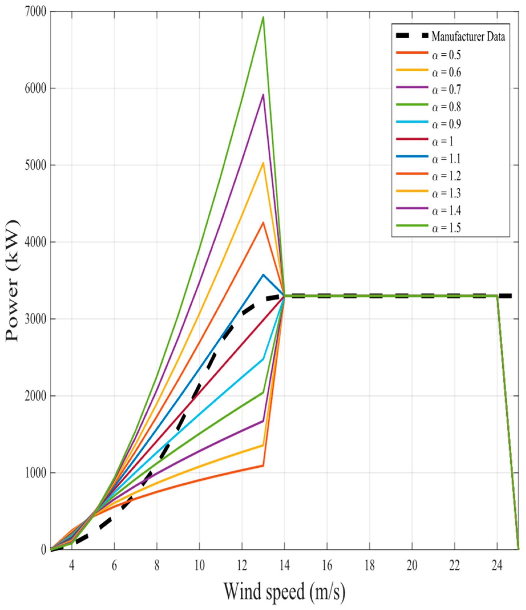
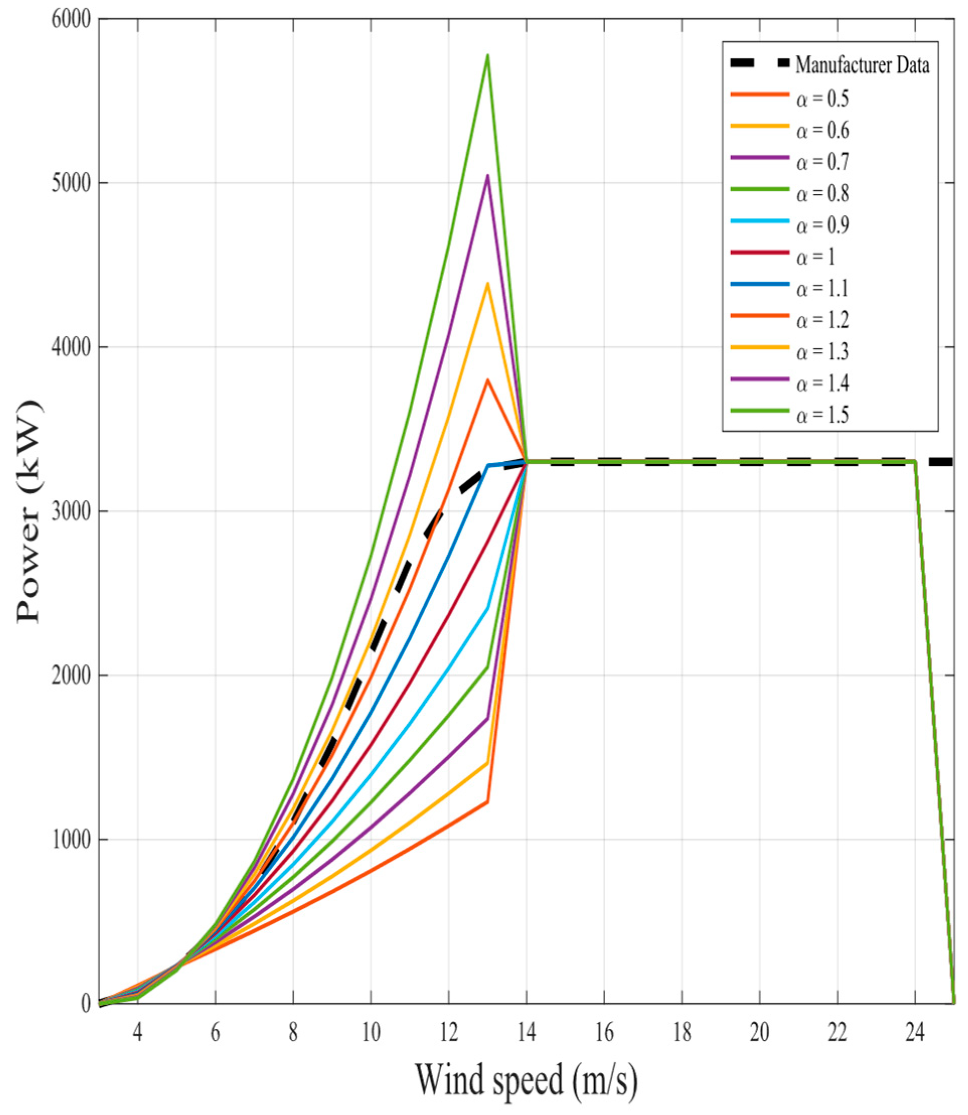
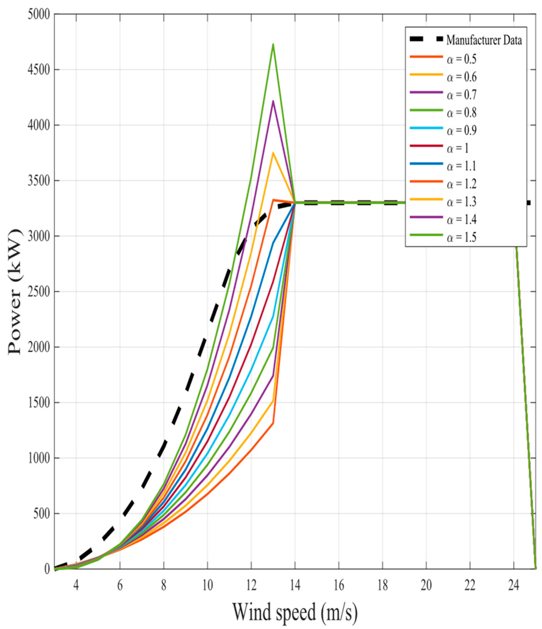
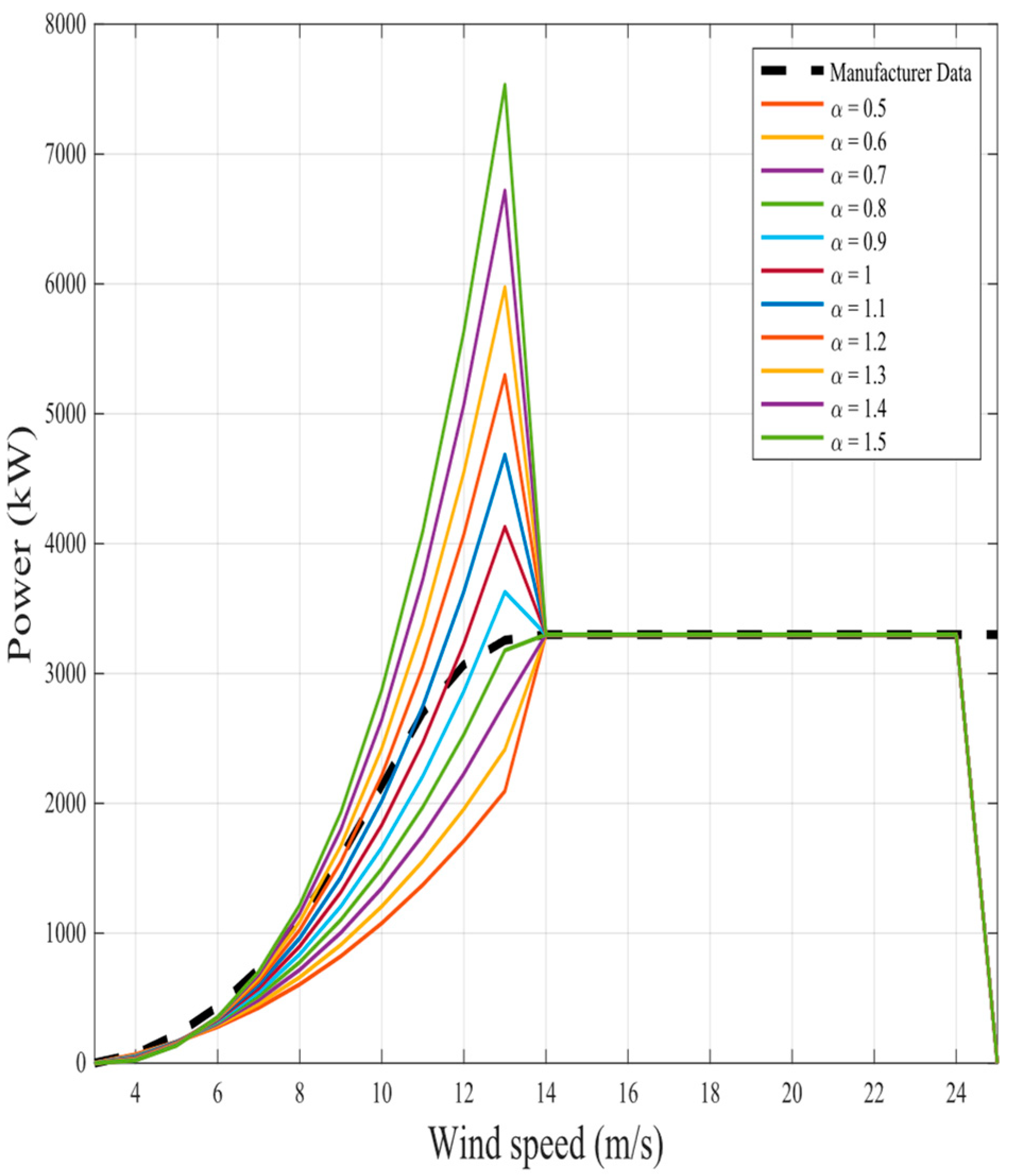
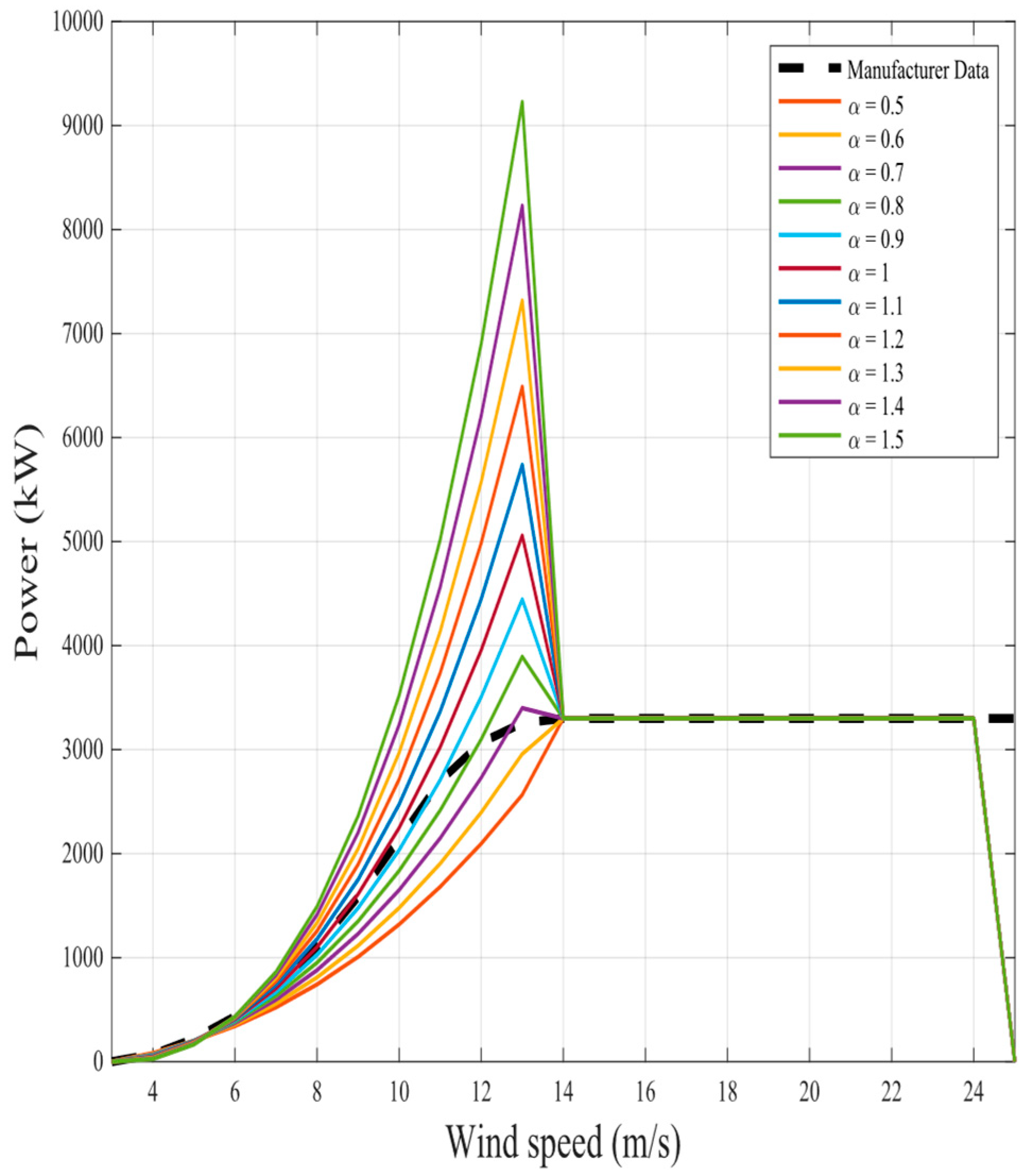
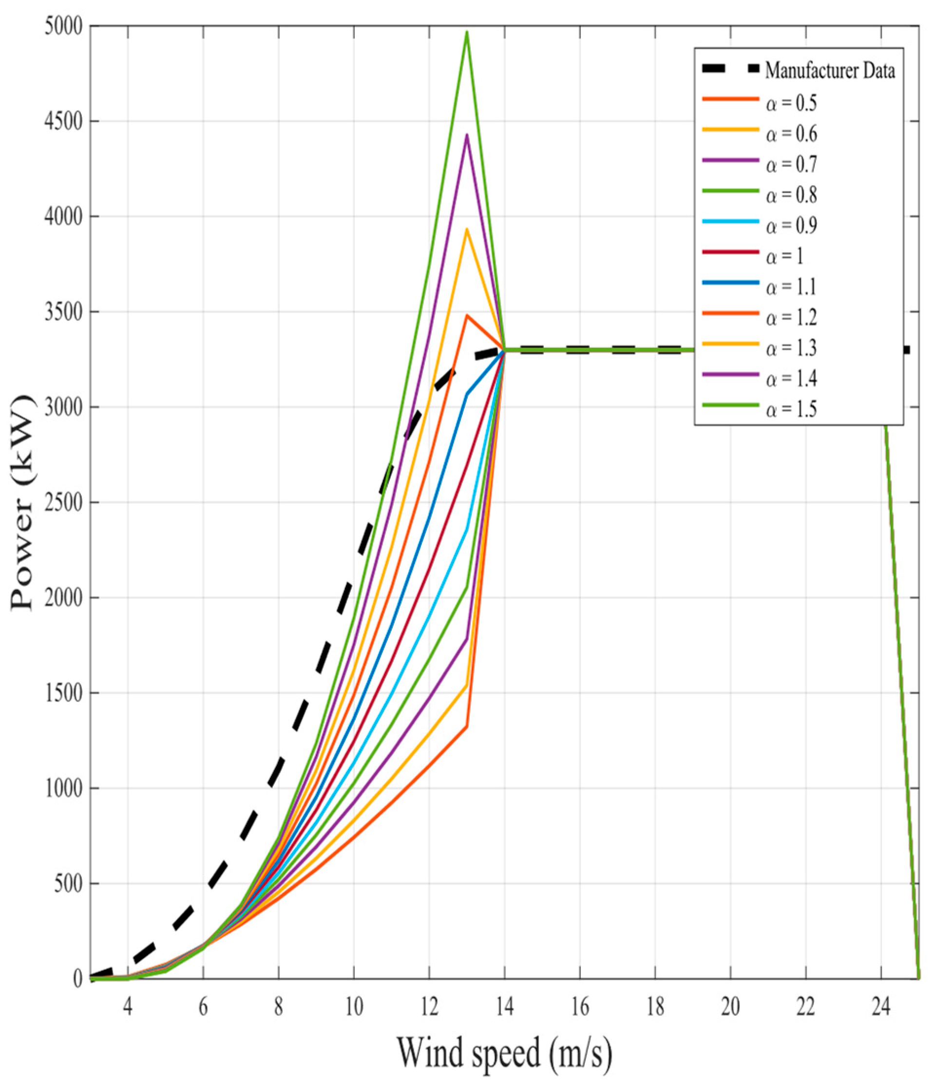
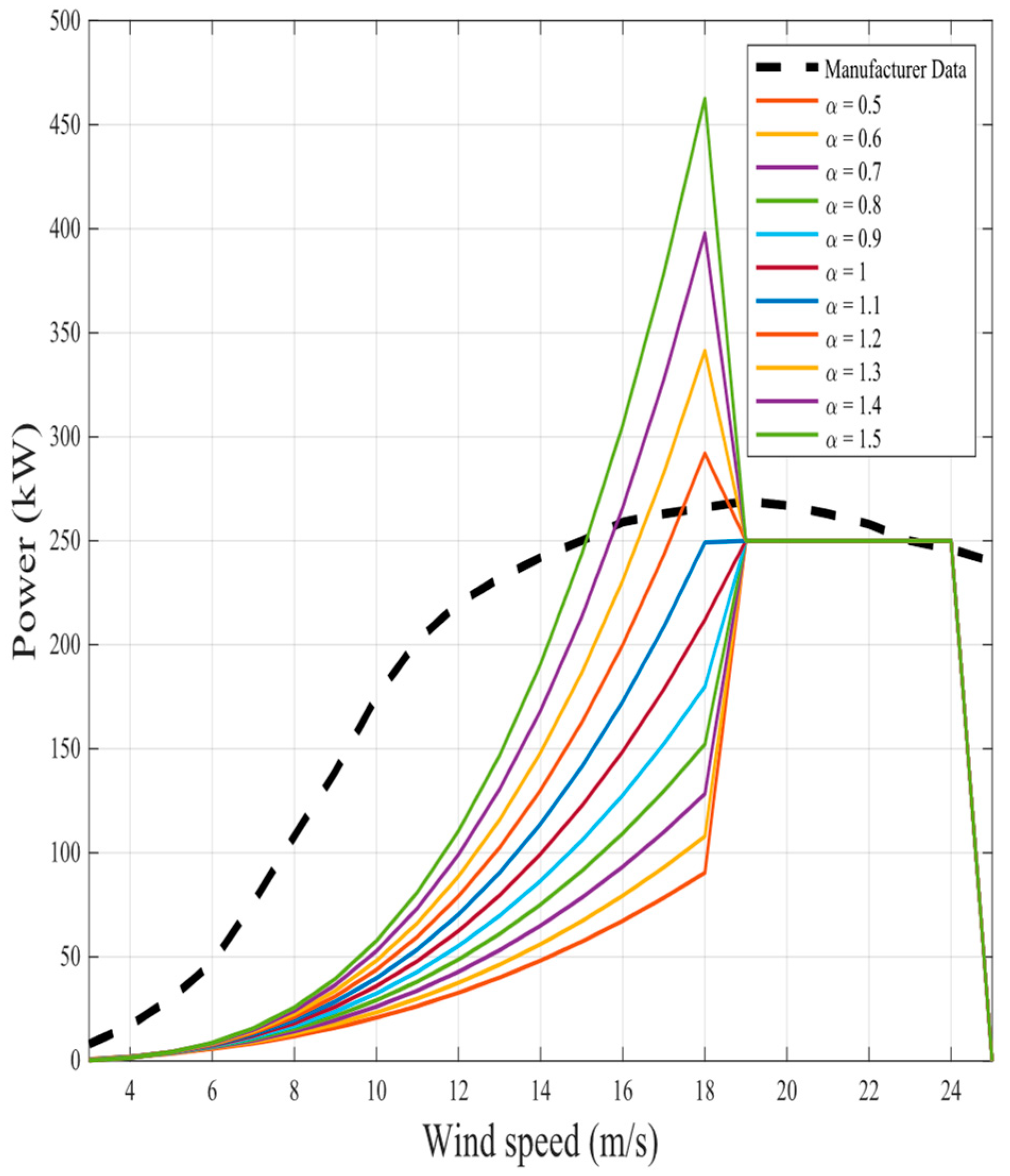
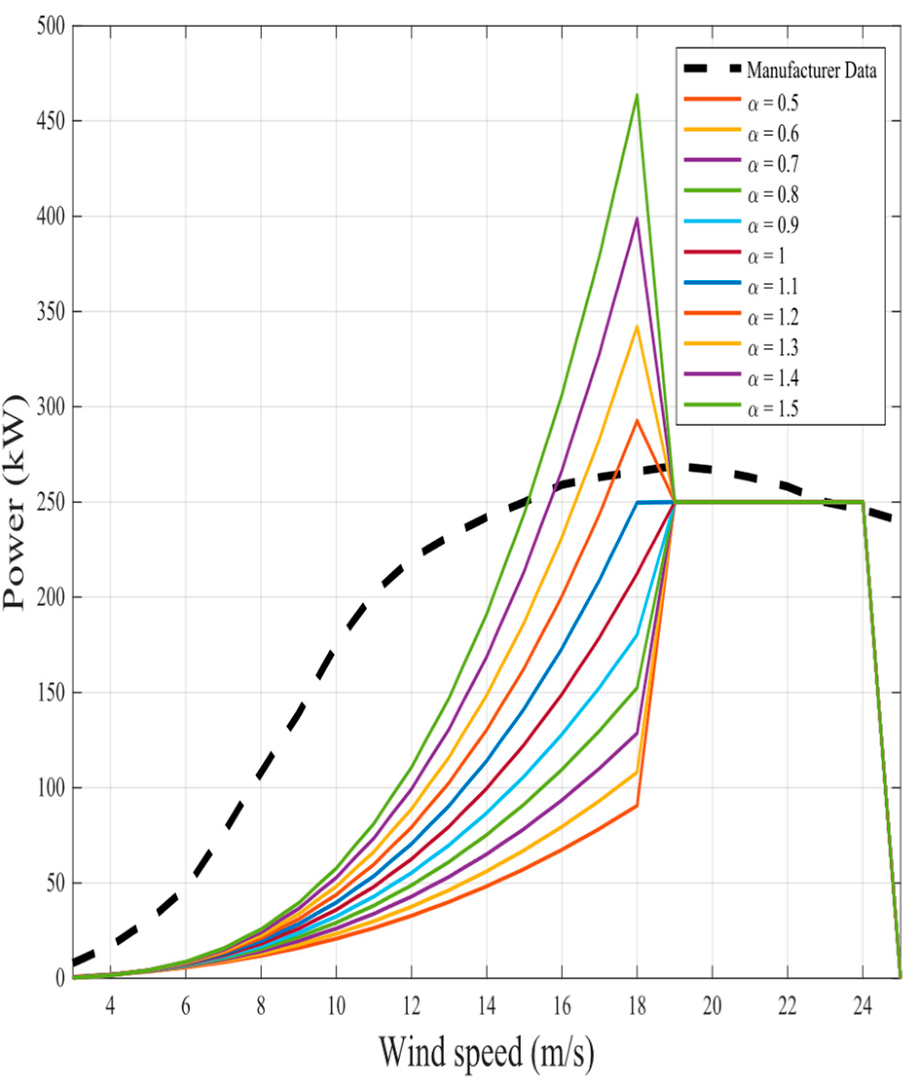
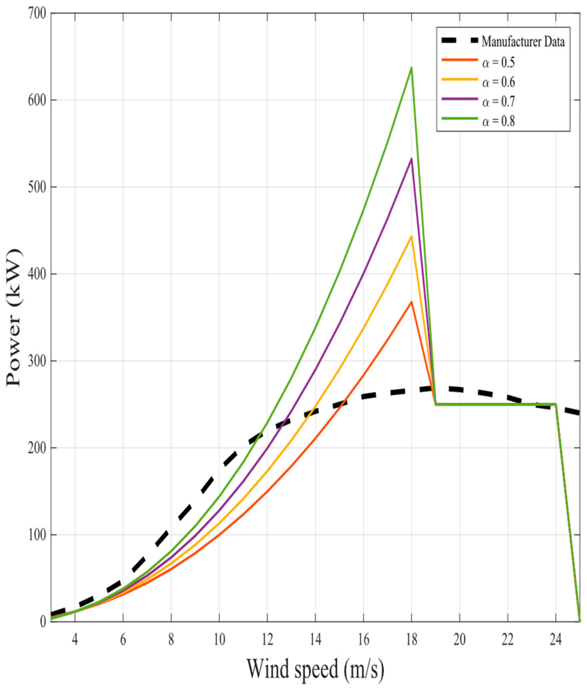
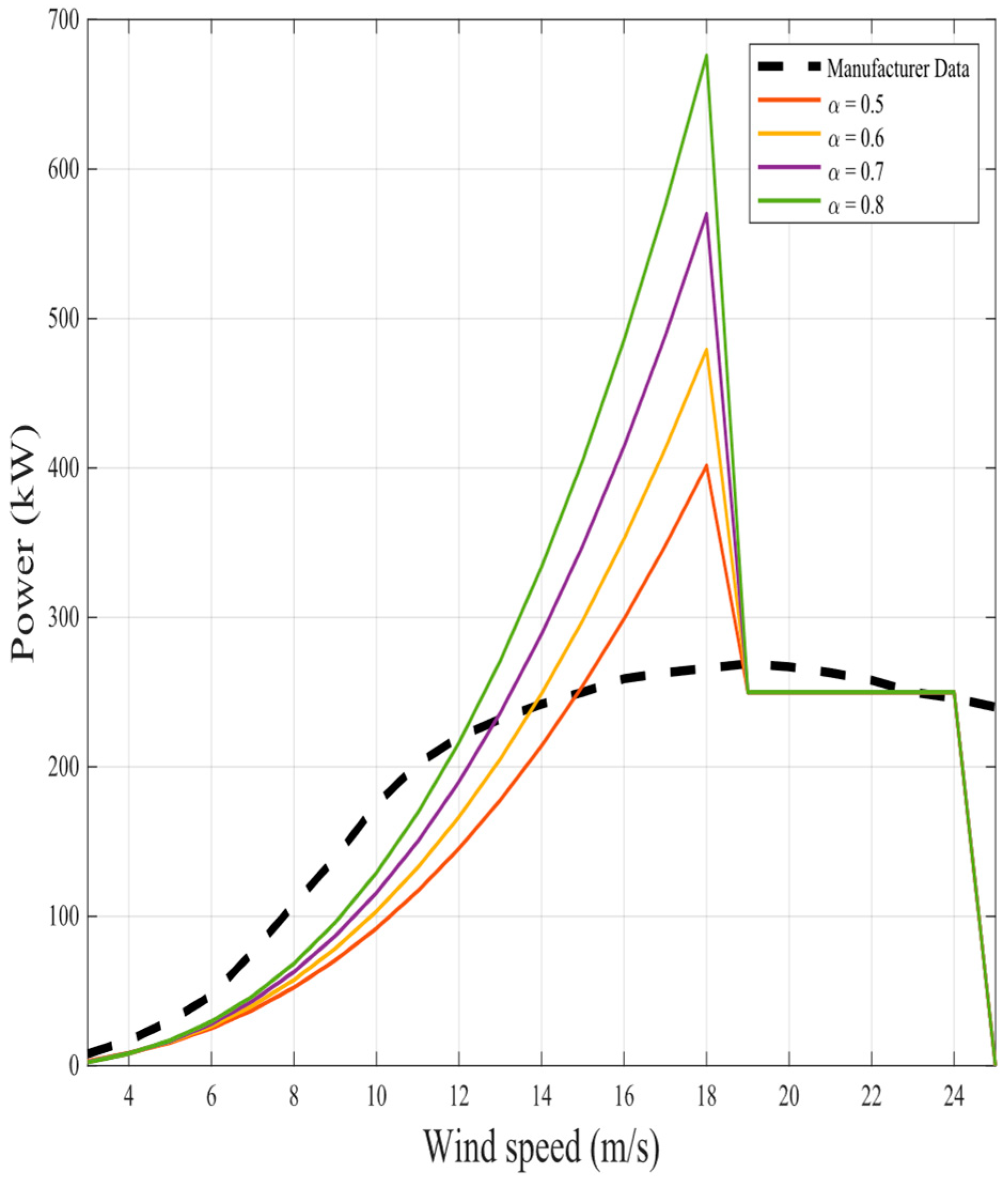
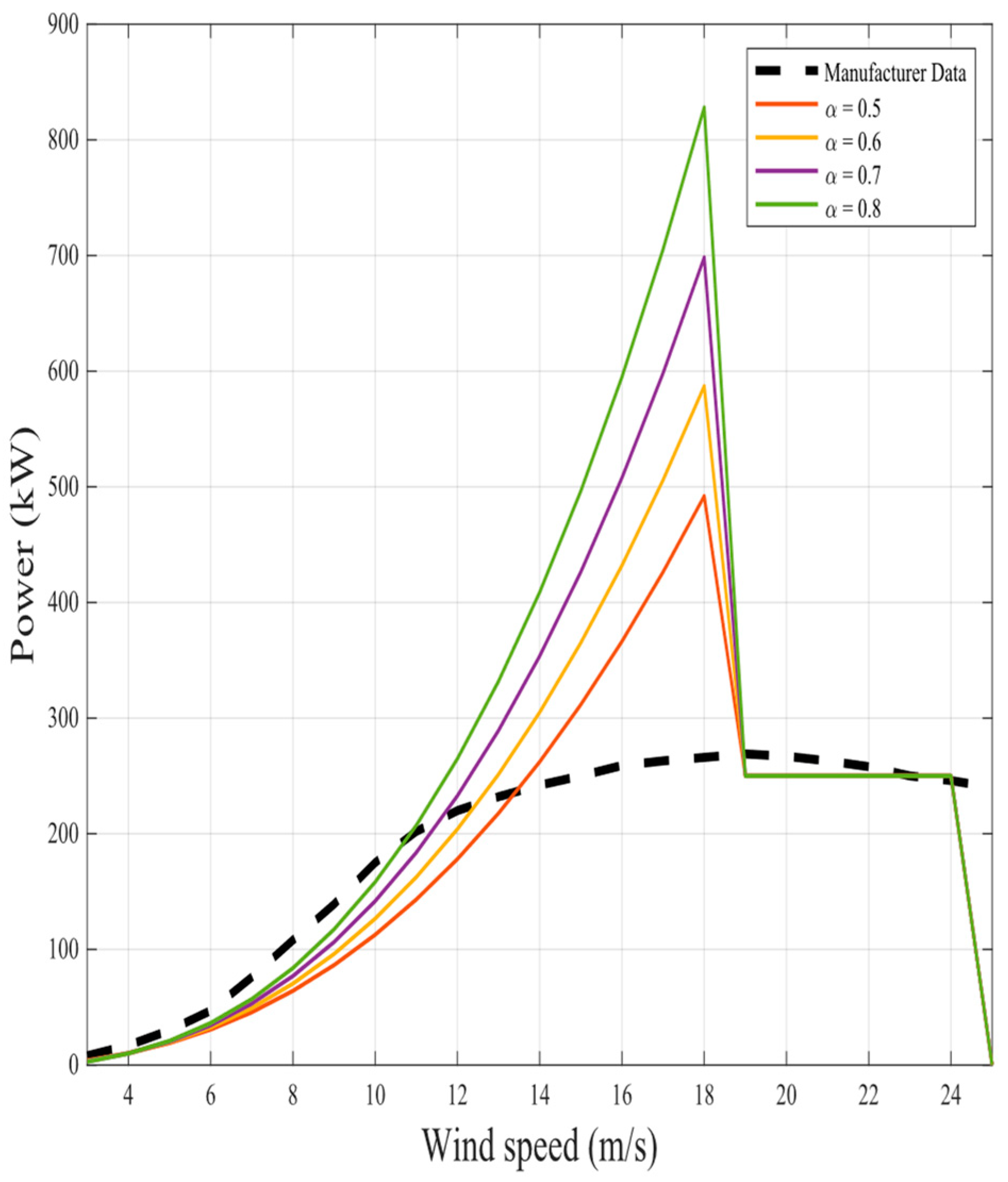
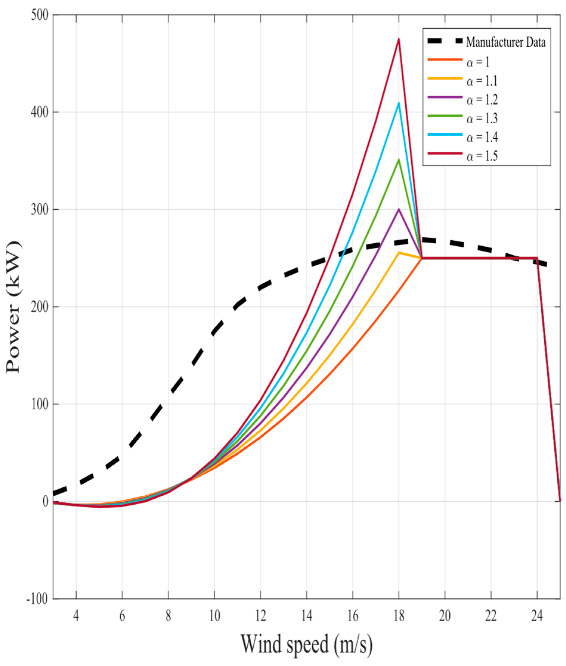
The representation of the proposed nine fractional mathematical models at different $\alpha$ for the same two wind turbines in original models is shown in Figure 6, Figure 7, Figure 8, Figure 9, Figure 10, Figure 11, Figure 12, Figure 13, Figure 14, Figure 15, Figure 16, Figure 17, Figure 18, Figure 19, Figure 20, Figure 21, Figure 22 and Figure 23. The results illustrate as the $\alpha$ value increases in each model, more overshoot happens from the rated power. The nearest curves to the manufacturer power curve occur at around $\alpha =1$.

Table 4. Summary of MAPE for fractional mathematical models for wind turbine model N100/3300.

α Mathematical Model	0.5	0.6	0.7	0.8	0.9	1	1.1	1.2	1.3	1.4	1.5
1. Linear	73.33	66.69	60.83	54.39	49.23	45.10	46.21	55.90	66.58	78.33	91.21
2. Quadratic	48.44	42.54	36.15	29.28	21.93	14.58	8.90	6.91	12.31	22.13	32.49
3. Cubic type-I	60.88	58.35	55.62	52.67	49.47	46.02	42.30	38.72	37.02	36.03	36.55
4. Cubic type-II	60.26	57.69	54.92	51.92	48.67	45.17	41.39	38.06	36.34	35.65	36.18
5. General	49.68	44.64	40.81	36.99	32.83	28.30	23.37	20.27	19.14	20.34	25.61
6. Exponential	33.61	26.76	19.55	12.09	9.09	8.68	14.61	24.16	34.31	45.00	56.24
7. Power coefficient	37.66	33.63	29.27	24.57	21.76	20.40	20.88	24.12	30.01	37.73	46.29
8. Approximated power coefficient	27.60	20.64	14.24	11.72	11.60	15.30	23.55	33.02	43.07	53.73	64.99
9. Polynomial	65.18	62.57	59.73	56.65	53.33	49.76	45.94	43.23	41.66	42.10	43.15

presents a comparative summary of MAPE for the proposed fractional models used to estimate the P-V characteristics of the N100/3300 wind turbine as an example. The table demonstrates the performance of nine different models with varying α, ranging from 0.5 to 1.5. As shown, the MAPE values reflect the accuracy of each model at different fractional orders, with lower values indicating better performance. Notably, the exponential model at α = 1 (integer order) yields the lowest MAPE (8.68%), signifying the highest accuracy among the models evaluated. In contrast, the linear model at α = 1.5 exhibits the highest MAPE (91.21%), marking the least accurate result. Overall, the table provides insight into how varying the α affects the predictive accuracy of each model, enabling a nuanced understanding of their behaviour in wind turbine power curve modelling.

Table 5. Summary of correlation coefficient for fractional mathematical models for wind turbine model N100/3300.

α Mathematical Model	0.5	0.6	0.7	0.8	0.9	1	1.1	1.2	1.3	1.4	1.5
1. Linear	0.9517	0.9625	0.9715	0.9787	0.9844	0.9886	0.9916	0.9935	0.9945	0.9945	0.9939
2. Quadratic	0.9918	0.9927	0.9932	0.9934	0.9930	0.9923	0.9911	0.9895	0.9875	0.9852	0.9826
3. Cubic type-I	0.9865	0.9848	0.9828	0.9806	0.9782	0.9757	0.9729	0.9699	0.9668	0.9636	0.9602
4. Cubic type-II	0.9865	0.9848	0.9828	0.9806	0.9782	0.9757	0.9729	0.9699	0.9668	0.9636	0.9602
5. General	0.9929	0.9925	0.9917	0.9906	0.9892	0.9875	0.9855	0.9832	0.9806	0.9778	0.9747
6. Exponential	0.9906	0.9894	0.9880	0.9863	0.9843	0.9821	0.9796	0.9769	0.9740	0.9709	0.9677
7. Power coefficient	0.9865	0.9848	0.9828	0.9806	0.9782	0.9757	0.9729	0.9699	0.9668	0.9636	0.9602
8. Approximated power coefficient	0.9865	0.9848	0.9828	0.9806	0.9782	0.9757	0.9729	0.9699	0.9668	0.9636	0.9602
9. Polynomial	0.9938	0.9923	0.9903	0.9878	0.9849	0.9816	0.9780	0.9742	0.9701	0.9659	0.9615

provides a detailed summary of the correlation coefficients for the proposed fractional models used to estimate the P-V characteristics of the N100/3300 wind turbine as an example. The correlation coefficient values presented in the table correspond to different α values ranging from 0.5 to 1.5. A higher correlation coefficient reflects a stronger linear relationship between the predicted and actual data. As observed in the table, the linear model consistently exhibits one of the highest R values across various fractional orders, reaching up to 0.9945 at α = 1.3. In contrast, the cubic models show slightly lower correlation values, particularly as α increases beyond 1.1. Notably, the general model maintains a high level of accuracy, with R = 0.9929 at α = 0.5, further validating the effectiveness of fractional differentiation in enhancing the model’s performance.

The results of the proposed fractional models’ performance evaluation are illustrated in

Table 6. Summary of correlation coefficient and MAPE values for fractional mathematical models.

Mathematical Model	$\mathit{\alpha }$	Mean of the Correlation Coefficient	Mean of MAPE		Rank
		$\mathit{R}$	MAPE	% Improvement
1. Linear	1	0.9830	49.57	0	9
2. Quadratic	1.2	0.9816	23.62	22.62	3
3. Cubic type-I	1.4	0.9522	41.36	2.62	7
4. Cubic type-II	1.4	0.9523	41.02	17.60	6
5. General	1.3	0.9712	27.74	27.74	4
6. Exponential	0.9	0.9710	20.54	16.05	1
7. Power coefficient	0.9	0.9635	27.55	1.25	5
8. Approximated power coefficient	0.8	0.9663	22.38	47.44	2
9. Polynomial	1.3	0.9583	47.44	12.6	8

, where for each model, the $\alpha$ at which the model gives the best performance is stated, and also the percentage improvement compared to the original model for MAPE is calculated. The score for each model and its rank are shown in

Table 7. Fractional mathematical models’ AHP scores with their ranking.

Mathematical Model	AHP Score	Rank
1. Linear	0.0904	9
2. Quadratic	0.1275	3
3. Cubic type-I	0.0953	7
4. Cubic type-II	0.0957	6
5. General	0.1163	4
6. Exponential	0.1375	1
7. Power coefficient	0.1163	5
8. Approximated power coefficient	0.1305	2
9. Polynomial	0.0905	8

. The results show that the best model is the exponential model at $\alpha =0.9$, with a percentage improvement in MAPE compared to the original exponential model by $16.05\%$, and the worst model is the linear model $\alpha =1$ (the original linear model). The rank of models differs from original models to fractional models. The fractional model obtains improvements in MAPE that reach around 44% in the approximated power coefficient model; however, it fails to give better results than the original linear model.

The R and MAPE values of the nine fractional mathematical models radar charts, respectively, are shown in Figure 24, where the linear model has the highest correlation coefficient at $\alpha =1.3$, while cubic type I, power coefficient, and approximated power coefficient models have the lowest R at $\alpha =0.5$. The MAPE is the lowest value for the exponential model at $\alpha =0.9$ and the highest value for the linear model at $\alpha =1$ (original linear model).

Based on the Weibull and gamma distributions, the values of RE’s mean and standard deviation are calculated. The value of $\mathit{\alpha }$ at which each model gives the best accuracy, determined as RE, is to be minimized. These results are illustrated in

Table 8. Summary of relative error: mean and standard deviation for mathematical models.

Mathematical Model	Weibull Distribution				Gamma Distribution
	Relative Error		$\mathit{\alpha }$	Rank	Relative Error		$\mathit{\alpha }$	Rank
	Mean	Standard Deviation			Mean	Standard Deviation
Linear	22.53	13.65	0.5	6	20.82	13.3	0.5	6
Quadratic	17.67	10.42	0.5	5	16.36	10.71	0.5	5
Cubic type-I	15.52	10.3	0.5	1	14.7	10.38	0.5	1
Cubic type-II	15.66	10.34	0.5	2	14.78	10.74	0.5	2
General	16.82	10.23	0.5	4	15.42	10.81	0.5	4
Exponential	31.54	16.09	0.5	9	30.89	14.41	0.5	9
Power coefficient	27.82	15.51	0.5	7	26.21	14.09	0.5	7
Approximated power coefficient	28.96	12.41	0.5	8	27.76	11.1	0.5	8
Polynomial	16.01	10.37	0.5	3	14.98	10.67	0.5	3

. It is evident that the cubic type-I model at $\mathit{\alpha }=0.5$ has the smallest values of mean RE; consequently, it is regarded as the most accurate mathematical model for estimating capacity factor. In contrast, the exponential model at $\mathit{\alpha }=0.5$ has the highest values of mean RE; thus, it can be considered the worst model for estimating capacity factor. The gamma distribution gives lower RE than the Weibull distribution, which means it is more suitable for capacity factor estimation at this site.

6. Conclusions and Future Work

This paper introduced nine novel fractional mathematical models for power curve modelling of wind turbines using the Riemann–Liouville fractional integral. Additionally, it calculated the capacity factor based on gamma and Weibull PDFs. In addition, it examined nine mathematical models for modelling wind turbine power curves to determine which one is the most accurate and at which order differentiation occurs. Utilizing statistical criteria, the suggested fractional models’ accuracy was assessed, including mean percentage absolute error, correlation coefficient for power curve accuracy, and relative error for capacity factor accuracy. From this study’s findings, the following can be concluded:

•

The exponential model at $\mathit{\alpha }=0.9$ is the best-fitting fractional mathematical model of the power curve with manufacturers’ power curves in the range of $\left[{\mathit{v}}_{\mathit{c}\mathit{i}},{\mathit{v}}_{\mathit{r}}\right),$ given that it has the greatest AHP score among the fractional mathematical models of the power curve that have been provided.

•

The cubic type-I model yielded the lowest relative error, estimated using Weibull and gamma distributions, of all mathematical models, making it the most accurate model for calculating capacity factor at $\mathit{\alpha }=0.5$.

•

The gamma distribution is more suitable in capacity factor estimation for the selected site as it gives less relative error than the Weibull distribution.

•

The linear model at $\mathit{\alpha }=1$ was found to be the least accurate model in power curve modelling. In contrast, the exponential model at $\mathit{\alpha }=0.5$ was the least accurate model in capacity factor estimation.

Future studies may focus on involving the hub height in capacity factor estimation, also using optimization techniques to determine the exact $\mathit{\alpha }$ that gives the best accuracy and determining the order of power output curve in the general model, measuring the precise values of ${\mathit{C}}_{\mathit{p},\mathit{e}\mathit{q}},{\mathit{C}}_{\mathit{p},\mathit{m}\mathit{a}\mathit{x}}$ to obtain better results and involve Brownian motion in any stochastic process that could occur.

References

1. Zayas-Gato, F.; Jove, E.; Casteleiro-Roca, J.-L.; Quintián, H.; Pérez-Castelo, F.J.; Piñón-Pazos, A.; Arce, E.; Calvo-Rolle, J.L. Intelligent model for active power prediction of a small wind turbine. Log. J. IGPL 2023, 31, 785–803. [Google Scholar] [CrossRef]
2. Liu, J.; Song, D.; Li, Q.; Yang, J.; Hu, Y.; Fang, F.; Joo, Y.H. Life cycle cost modelling and economic analysis of wind power: A state of art review. Energy Convers. Manag. 2023, 277, 116628. [Google Scholar] [CrossRef]
3. Wilberforce, T.; Olabi, A.G.; Sayed, E.T.; Alalmi, A.H.; Abdelkareem, M.A. Wind turbine concepts for domestic wind power generation at low wind quality sites. J. Clean Prod. 2023, 394, 136137. [Google Scholar] [CrossRef]
4. Marti-Puig, P.; Hernández, J.Á.; Solé-Casals, J.; Serra-Serra, M. Enhancing Reliability in Wind Turbine Power Curve Estimation. Appl. Sci. 2024, 14, 2479. [Google Scholar] [CrossRef]
5. Bilendo, F.; Meyer, A.; Badihi, H.; Lu, N.; Cambron, P.; Jiang, B. Applications and Modeling Techniques of Wind Turbine Power Curve for Wind Farms—A Review. Energies 2022, 16, 180. [Google Scholar] [CrossRef]
6. Teyabeen, A.; Akkari, F.; Jwaid, A. Mathematical Modelling of Wind Turbine Power Curve. Int. J. Simul. Syst. Sci. Technol. 2019. [Google Scholar] [CrossRef]
7. Carrillo, C.; Montaño, A.F.O.; Cidrás, J.; Díaz-Dorado, E. Review of power curve modelling for wind turbines. Renew. Sustain. Energy Rev. 2013, 21, 572–581. [Google Scholar] [CrossRef]
8. Prema, V.; Bhaskar, M.S.; Almakhles, D.; Gowtham, N.; Rao, K.U. Critical Review of Data, Models and Performance Metrics for Wind and Solar Power Forecast. IEEE Access 2022, 10, 667–688. [Google Scholar] [CrossRef]
9. Capelletti, M.; Raimondo, D.M.; De Nicolao, G. Wind power curve modeling: A probabilistic Beta regression approach. Renew. Energy 2024, 223, 119970. [Google Scholar] [CrossRef]
10. Jung, C.; Schindler, D. Efficiency and effectiveness of global onshore wind energy utilization. Energy Convers. Manag. 2023, 280, 116788. [Google Scholar] [CrossRef]
11. Dinçer, A.E.; Demir, A.; Yılmaz, K. Enhancing wind turbine site selection through a novel wake penalty criterion. Energy 2023, 283, 129096. [Google Scholar] [CrossRef]
12. Adel, W.; Elsonbaty, A.; Mahdy, A.M.S. On some recent advances in fractional order modeling in engineering and science. In Computation and Modeling for Fractional Order Systems; Elsevier: Amsterdam, The Netherlands, 2024; pp. 169–197. [Google Scholar] [CrossRef]
13. Singh, A.P.; Bingi, K. Applications of Fractional-Order Calculus in Robotics. Fractal Fract. 2024, 8, 403. [Google Scholar] [CrossRef]
14. Teodoro, G.S.; Machado, J.A.T.; de Oliveira, E.C. A review of definitions of fractional derivatives and other operators. J. Comput. Phys. 2019, 388, 195–208. [Google Scholar] [CrossRef]
15. Valério, D.; Ortigueira, M.D.; Lopes, A.M. How Many Fractional Derivatives Are There? Mathematics 2022, 10, 737. [Google Scholar] [CrossRef]
16. Khan, M.B.; Guirao, J.L.G. Riemann Liouville fractional-like integral operators, convex-like real-valued mappings and their applications over fuzzy domain. Chaos Solitons Fractals 2023, 177, 114196. [Google Scholar] [CrossRef]
17. Noor, A.; Bazuhair, M.; El-Beltagy, M. Analytical and Computational Analysis of Fractional Stochastic Models Using Iterated Itô Integrals. Fractal Fract. 2023, 7, 575. [Google Scholar] [CrossRef]
18. Scherer, R.; Kalla, S.L.; Tang, Y.; Huang, J. The Grünwald–Letnikov method for fractional differential equations. Comput. Math. Appl. 2011, 62, 902–917. [Google Scholar] [CrossRef]
19. Fallahgoul, H. Riemann-Liouville Fractional Derivative. In Fractional Calculus and Fractional Processes with Applications to Financial Economics; Academic Press: Cambridge, MA, USA, 2017. [Google Scholar]
20. Medveď, M.; Brestovanská, E. Differential Equations with Tempered Ψ-Caputo Fractional Derivative. Math. Model. Anal. 2021, 26, 631–650. [Google Scholar] [CrossRef]
21. Alharthi, A.S. A new probabilistic model with applications to the wind speed energy data sets. Alex. Eng. J. 2024, 86, 67–78. [Google Scholar] [CrossRef]
22. Ding, Y.; Ye, X.-W.; Guo, Y.; Zhang, R.; Ma, Z. Probabilistic method for wind speed prediction and statistics distribution inference based on SHM data-driven. Probabilistic Eng. Mech. 2023, 73, 103475. [Google Scholar] [CrossRef]
23. Wadi, M. Five different distributions and metaheuristics to model wind speed distribution. J. Therm. Eng. 2021, 7, 1898–1920. [Google Scholar] [CrossRef]
24. Suwarno, S.; Yusuf, I.; Irwanto, M.; Hiendro, A. Analysis of wind speed characteristics using different distri bution models in Medan City, Indonesia. Int. J. Power Electron. Drive Syst. (IJPEDS) 2021, 12, 1102. [Google Scholar] [CrossRef]
25. Hasan, W.S.A.; Hassan, A.S.M.; Shukri, M.A. Assessing the performance of several numerical methods for estimating Weibull parameters for Wind Energy Applications: A case study of Al-Hodeidah in Yemen. Energy Rep. 2023, 10, 2725–2739. [Google Scholar] [CrossRef]
26. Mathew, S. Wind energy: Fundamentals, Resource Analysis and Economics; Springer-Verlag: New York, NY, USA; Berlin/Heidelberg, Germany, 2006. [Google Scholar]
27. Khan, M.G.M.; Ahmed, M.R. Bayesian method for estimating Weibull parameters for wind resource assessment in a tropical region: A comparison between two-parameter and three-parameter Weibull distributions. Wind. Energy Sci. 2023, 8, 1277–1298. [Google Scholar] [CrossRef]
28. Norrulashikin, S.M.; Kamisan, N.A.B.; Nor, S.R.M. Data fitting distribution for wind speed in Mersing, Johor. AIP Conf. Proc. 2024, 2895, 090012. [Google Scholar] [CrossRef]
29. Chiodo, E.; Diban, B.; Mazzanti, G.; De Angelis, F. A Review on Wind Speed Extreme Values Modeling and Bayes Estimation for Wind Power Plant Design and Construction. Energies 2023, 16, 5456. [Google Scholar] [CrossRef]
30. Karim, F.K.; Khafaga, D.S.; Eid, M.M.; Towfek, S.K.; Alkahtani, H.K. A Novel Bio-Inspired Optimization Algorithm Design for Wind Power Engineering Applications Time-Series Forecasting. Biomimetics 2023, 8, 321. [Google Scholar] [CrossRef]
31. Ahmed, M.A.; Kang, Y.C.; Kim, Y.-C. Modeling and simulation of ICT network architecture for cyber-physical wind energy system. In Proceedings of the 2015 IEEE International Conference on Smart Energy Grid Engineering (SEGE), Oshawa, ON, Canada, 17–19 August 2015; IEEE: New York, NY, USA, 2015; pp. 1–6. [Google Scholar] [CrossRef]
32. Chang, T.-P.; Liu, F.-J.; Ko, H.-H.; Cheng, S.-P.; Sun, L.-C.; Kuo, S.-C. Comparative analysis on power curve models of wind turbine generator in estimating capacity factor. Energy 2014, 73, 88–95. [Google Scholar] [CrossRef]
33. Avila-Rodriguez, V.; Leon-Zerpa, F.; Quintana-Hernandez, J.J.; Ramos-Martin, A. Modeling the Dynamics of Supercapacitors by Means of Riemann–Liouville Integral Definition. Electricity 2024, 5, 491–525. [Google Scholar] [CrossRef]
34. Albadi, M.H.; El-Saadany, E.F. Wind Turbines Capacity Factor Modeling—A Novel Approach. IEEE Trans. Power Syst. 2009, 24, 1637–1638. [Google Scholar] [CrossRef]
35. Albadi, M.H.; El-Saadany, E.F. Optimum turbine-site matching. Energy 2010, 35, 3593–3602. [Google Scholar] [CrossRef]
36. Goudarzi, A.; Davidson, I.E.; Ahmadi, A.; Venayagamoorthy, G.K. Intelligent analysis of wind turbine power curve models. In Proceedings of the 2014 IEEE Symposium on Computational Intelligence Applications in Smart Grid (CIASG), Orlando, FL, USA, 9–12 December 2014; IEEE: New York, NY, USA, 2014; pp. 1–7. [Google Scholar] [CrossRef]
37. Libii, J.N. Comparing the calculated coefficients of performance of a class of wind turbines that produce power between 330 kW and 7,500 kW. World Trans. Eng. Technol. Educ. 2013, 11, 36–40. [Google Scholar]
38. Vennell, R. Exceeding the Betz limit with tidal turbines. Renew. Energy 2013, 55, 277–285. [Google Scholar] [CrossRef]
39. Wen, J.; Zheng, Y.; Donghan, F. A review on reliability assessment for wind power. Renew. Sustain. Energy Rev. 2009, 13, 2485–2494. [Google Scholar] [CrossRef]
40. Nasery, P.; Ezzat, A.A. Yaw-adjusted wind power curve modeling: A local regression approach. Renew. Energy 2023, 202, 1368–1376. [Google Scholar] [CrossRef]
41. Sousa, J.; Lagarto, J.; Camus, C.; Viveiros, C.; Barata, F.; Silva, P.; Alegria, R.; Paraíba, O. Renewable energy communities optimal design supported by an optimization model for investment in PV/wind capacity and renewable electricity sharing. Energy 2023, 283, 128464. [Google Scholar] [CrossRef]
42. TheWindPower. Goldwind, 8 March 2022. Available online: https://www.thewindpower.net/manufacturer_en_71_goldwind.php (accessed on 15 August 2024).
43. TheWindPower. Nordex, 19 July 2023. Available online: https://www.thewindpower.net/manufacturer_en_8_nordex.php (accessed on 15 August 2024).
44. TheWindPower. Gamesa, 4 June 2018. Available online: https://www.thewindpower.net/manufacturer_en_4_gamesa.php (accessed on 15 August 2024).
45. Mayola, L.; Afdhal, M.; Yuhandri, M.H. Analytical Hierarchy Process (AHP) dalam Seleksi Penerimaan Mahasiswa Baru. J. KomtekInfo 2023, 10, 81–86. [Google Scholar] [CrossRef]
46. Zobaa, A.M.; Aleem, S.H.E.A.; Youssef, H.K.M. Bi-Level damped double-tuned harmonic passive filters design: Multi-criteria decision-making analysis. Ain Shams Eng. J. 2023, 14, 102082. [Google Scholar] [CrossRef]
Figure 1. Typical power curve of a wind turbine.
Fractalfract 08 00656 g001
Figure 2. Graphical abstract of the research.
Fractalfract 08 00656 g002
Figure 3. Histogram of the 36 selected wind turbines for wind turbine characteristics: (a) rated power; (b) cut-in wind speed; (c) rated wind speed; (d) cut-out wind speed.
Fractalfract 08 00656 g003
Figure 4. Representation of all original mathematical models for power curve of wind turbine models (a) N100/3300; (b) N29/250.
Fractalfract 08 00656 g004
Figure 5. Representation of statistical criteria of all original mathematical models for power curve of wind turbine: (a) correlation coefficient; (b) MAPE.
Fractalfract 08 00656 g005
Figure 6. Representation of linear model for wind turbine model N100/3300.
Fractalfract 08 00656 g006
Figure 7. Representation of quadratic model for wind turbine model N100/3300.
Fractalfract 08 00656 g007
Figure 8. Representation of cubic type-I model for wind turbine model N100/3300.
Fractalfract 08 00656 g008
Figure 9. Representation of cubic type-II model for wind turbine model N100/3300.
Fractalfract 08 00656 g009
Figure 10. Representation of general model for wind turbine model N100/3300.
Fractalfract 08 00656 g010
Figure 11. Representation of exponential model for wind turbine model N100/3300.
Fractalfract 08 00656 g011
Figure 12. Representation of power-coefficient-based model for wind turbine model N100/3300.
Fractalfract 08 00656 g012
Figure 13. Representation of approximated power-coefficient-based model for wind turbine model N100/3300.
Fractalfract 08 00656 g013
Figure 14. Representation of polynomial model for wind turbine model N100/3300.
Fractalfract 08 00656 g014
Figure 15. Representation of linear model for wind turbine model N29/250.
Fractalfract 08 00656 g015
Figure 16. Representation of quadratic model for wind turbine model N29/250.
Fractalfract 08 00656 g016
Figure 17. Representation of cubic type-I model for wind turbine model N29/250.
Fractalfract 08 00656 g017
Figure 18. Representation of cubic type-II model for wind turbine model N29/250.
Fractalfract 08 00656 g018
Figure 19. Representation of general model for wind turbine model N29/250.
Fractalfract 08 00656 g019
Figure 20. Representation of exponential model for wind turbine model N29/250.
Fractalfract 08 00656 g020
Figure 21. Representation of power-coefficient-based model for wind turbine model N29/250.
Fractalfract 08 00656 g021
Figure 22. Representation of approximated power-coefficient-based model for wind turbine model N29/250.
Fractalfract 08 00656 g022
Figure 23. Representation of polynomial model for wind turbine model N29/250.
Fractalfract 08 00656 g023
Figure 24. Representation of statistical criteria of all fractional mathematical models for power curve of wind turbine: (a) correlation coefficient; (b) MAPE.
Fractalfract 08 00656 g024