An Algorithm for the Solution of Integro-Fractional Differential Equations with a Generalized Symmetric Singular Kernel

Abstract

This work studies an integro-fractional differential equation (I-FrDE) with a generalized symmetric singular kernel. The scientific approach in this study was to transform the integro-differential equation (I-DE) into a mixed integral equation (MIE) with an Able kernel in fractional time and a generalized symmetric singular kernel in position. Additionally, the authors first set conditions on the singular kernels, whether related to time or position, and then transform the integral equation into an integral operator. Secondly, the solution is unique, which is proven by means of fixed-point theorems. In combination with the solution rules, the convergence of the solution is studied, and the error equation resulting from the solution is a stable error-integral influencer equation. Next, to solve this MIE, the authors apply a special technique to separate the variables and produce an integral equation in position with coefficients, in the form of an integral operator in time. As the most effective technique for resolving singular integral equations, the Toeplitz matrix method (TMM) is utilized to convert the integral equation into an algebraic system for the purpose of solving the position problem. The existence of a solution to the linear algebraic system in Banach space is then demonstrated. Lastly, certain applications where the functions of the generalized symmetric kernel are cubic or exponential and it assumes the logarithmic, Cauchy, or Carleman form are discussed. In each case, Maple 18 is also used to compute the error estimate.

1. Introduction

The utilization of fractional equations has rapidly broadened and diversified in a brief span of time. Previous research described the construction of fractional integro-differential equations (FrI-DEs) from electromagnetic waves in a dielectric material [1]. The authors in [2] have focused on the stability analysis of the RLC model by using Hadamard Fr-DEAs which have been transformed into an equivalent I-DE. Solutions to a specific type of Cauchy problem with integral conditions for FrI-DEs have been demonstrated to exist throughout. The use of fixed-point methods has also been demonstrated, as shown in references [3,4], where the authors studied the existence of a solution to FrI-DE using fixed-point theorems and the Banach concept, respectively. In [5], Hölder’s inequality and Schauder’s fixed point theorem were used to prove the existence and uniqueness of a mild solution for FrI-DEs with nonlocal initial conditions in Banach spaces.

Several writers are intrigued by various approaches for solving FrI-DEs. The authors in reference [6] employed fractional-order Euler functions to solve FrI-DEs. The introduction of the generalized hat functions and operational matrix in [7] aimed to address the solution of the FrI-DEs of Bratu type. The Volterra fractional integral equation (V-FrIE) was obtained from a linear I-DE [8]. The sinc-collocation approach was introduced in [9] as a solution for Volterra-Fredholm integro-differential equations (V-FI-DEs). The authors in [10] presented a Barycentric interpolation collocation method to solve FrF-VI-DE. The generalized monotone iterative technique was devised to solve the Caputo FrI-DEs of order $q$ in [11]. The Bernoulli polynomial approach was introduced in [12] as a solution of mixed-dimensional difference I-DEs with coefficients of variables. In [13], an analysis of spectrum relationships was conducted on an integral operator including a singular kernel. A fundamental theorem for spectral relations was derived, utilizing Chebyshev’s polynomials. The FIE was derived in [14], after using an asymptotic method to separate the variables in a mixed integral equation (MIE). Several numerical solutions have been applied to treat MIEs in [15,16,17,18,19].

Given the importance of applications of MIEs in various sciences such as mathematical physics, genetic engineering, communication issues in media mechanics, and other sciences, researchers’ interest has focused on how to study a mixed equation in space and position. Fractional time has been chosen to show its greatest effect in small times, and the position kernel has been chosen as discontinuous (singular) so that the study is broader and more comprehensive than the continuous kernels.

It is noted that in the previous papers that included fractional time, some authors used one of the following methods: semi-analytical or numerical methods in which the kernel is continuous. However, in this paper, the method of solving the problem differed by choosing a technique in separating the variables that transforms the part related to fractional time into an integral operator of an IE in position. Also, the authors’ choice of a singular kernel in the general form and the use of the TMM transformed the singular integrals in the equation into numerical integrals that are easy to solve.

This paper is organized as follows: we introduce the I-FrDE with a general form of a generalized symmetric singular kernel in position, under certain conditions in the space $L_2\left(-\mathrm{1,1}\right)\times C\left[0,T\right],T<1,$ where $T$ is the time. In Section 2, a MIE is derived from I-FrDE. Then, in Section 3, under certain conditions, the existence of a unique solution is proved using the Banach fixed point theorem. In Section 4, the stability of the solution and the convergence of the error are discussed. In Section 5, the separation of variables method is used to obtain an integral equation in position. The coefficients of the IE, in this case, are variable in time $t$, and the fractional $\mathsf{\alpha }$. In Section 6, TMM is used to transform the IE to a system of linear algebra equations (SLAEs). In Section 7, the existence of a unique solution of the SLAEs is proved, and its stability is considered. In Section 8, many numerical results are considered and obtained when the discontinuous kernel takes the general form of some different famous form. Additionally, each case’s related error is calculated. In Section 9, important points in this work are discussed. A general conclusion is given in Section 10.

2. Formulation of an Integro-Fractional Differential Equation

In this section, let us recall some basics of fractional integrals. To achieve the goal of this paper, the Riemann-Liouville fractional integral will be applied, taking advantage of the initial condition of I-FrDE.

Let $D^{\alpha }$ represent the Caputo defined fractional differential operator of order $\alpha$, $m-1<\alpha \le m$, defined by $D_a^{\alpha }f(x)=I_a^{m-\alpha }{D}^{m}f(x),$ wherein $D^m$ is the usual integral differential operator of order $m$ and $I^n$ is the Riemann-Liouville integer operator of order $n>0$.

Definition 1.

([7]). For all $x\in \left[a,b\right],\mathrm{f}(\mathrm{x})\in \mathrm{C}[\mathrm{a},\mathrm{b}]$, the left Riemann-Liouville fractional integral operator of order $\alpha >0$, of the function $f$, is defined as

$${}_{a}I_x^{\alpha }f\left(x\right)={\displaystyle \frac{1}{\mathsf{\Gamma }\left(\alpha \right)}}{\int }_a^x{\left(x-t\right)}^{\alpha -1}f\left(t\right)dt$$

(1)

In addition, we require the following necessary condition for $m-1<\alpha \le m,m\in \mathbb{N}$.

$$I^{\alpha }{D}^{\alpha }f\left(x\right)=f\left(x\right)-\sum _{i=0}^{m-1}{\displaystyle \frac{d^{i}f}{d{x}^i}}\left(0\right){\displaystyle \frac{x^i}{i!}},x>0,$$

(2)

here, $D^{\alpha }f\left(x\right)\in C[a,b]$.

Now, consider, in the space $L_2(-1,1)\times C\left[0,T\right],T<1,$ the I-FrDE is as follows:

$${\displaystyle \frac{{\partial }^{\alpha }}{\partial t^{\alpha }}}\left(\mu \mathsf{\Psi }\left(u,t\right)-f\left(u,t\right)\right)=\lambda h\left(t\right)\underset{-1}{\overset{1}{\int }}k\left(\left|\omega \left(u\right)-\omega \left(v\right)\right|\right)\mathsf{\Psi }\left(v,t\right)dv,0<\alpha <1,$$

(3)

with the condition $\mathsf{\Psi }\left(u,0\right)=\zeta \left(u\right).$

The above initial value problem (3) can be transformed using (2) to a Volterra-Fredholm integral equation (V-FIE) of the second kind with Able kernel in Volterra integral part.

$$\mu \mathsf{\Psi }(u,t)-{\displaystyle \frac{\lambda }{\mathsf{\Gamma }\left(\alpha \right)}}{\int }_0^t(t-\tau {)}^{\alpha -1}h\left(\tau \right){\int }_{-1}^{1}k\left(\left|\omega \left(u\right)-\omega \left(v\right)\right|\right){\omega }^{’}(v)\mathsf{\Psi }\left(v,\tau \right)dvd\tau =F\left(u,t\right),$$

(4)

where

$$F\left(u,t\right)=\mu \zeta \left(u\right)+f\left(u,t\right)-f\left(u,0\right).$$

It obvious that when $t=0$, Equation (2) will satisfy the initial condition $\mathsf{\Psi }\left(u,0\right)=\zeta \left(u\right).$ Special cases of the generalized singular kernel are as follows

Here, we discuss several special cases of the general symmetric singular kernel:

(i)

the weak singularity forms:

$$k\left(\left|\omega \left(u\right)-\omega \left(v\right)\right|\right)=\left\{\begin{array}{ll} g\left(x,y\right)\ln \left|\omega \left(x\right)-\omega \left(y\right)\right|,& (\mathrm{logarithmic}\mathrm{form})\\ g\left(x,y\right){\left|\omega \left(x\right)-\omega \left(y\right)\right|}^{-\beta },\hspace{1em}0\le \beta <1& (\mathrm{Carleman}\mathrm{function})\end{array}\right.$$

(ii)

$$k\left(\left|\omega \left(u\right)-\omega \left(v\right)\right|\right)={\displaystyle \frac{g\left(x,y\right)}{\left|\omega \left(x\right)-\omega \left(y\right)\right|}},\hspace{1em}\hspace{1em}\hspace{1em}\hspace{1em}\left(\mathrm{C}\mathrm{a}\mathrm{u}\mathrm{c}\mathrm{h}\mathrm{y} \mathrm{k}\mathrm{e}\mathrm{r}\mathrm{n}\mathrm{e}\mathrm{l}\right)$$

where, in general, $g(x,y)$ is a smooth function.

Generally, as special cases, let $\omega (x)=x$ in the two cases above, the solutions of which have been established by many authors via different numerical approaches; for an overview of such methods, see [7,9,12,13,18].

As novel cases in our numerical examples, we consider in application (1) that $\omega \left(x\right)=x^2$, whereas in application (2), we assume that $\omega \left(x\right)=e^x.$

3. The Existence and Uniqueness Solution of Integro-Fractional Differential Equation

To discuss the existence of a unique solution of the IE (4), we assume the following conditions:

(i)

The kernel of position $k\left(\left|\omega \left(u\right)-\omega \left(v\right)\right|\right),$ in the space $L_2(-\mathrm{1,1})$, satisfies the discontinuity condition

$${\int }_{-1}^1{\int }_{-1}^1|k\left(\left|\omega \left(u\right)-\omega \left(v\right)\right|\right){|}^2{\omega }^{’}(u){\omega }^{’}(v)dudv\le {\chi }^2,{\mathrm{w}}^{’}\left(\mathrm{x}\right)={\displaystyle \frac{dw}{dx}},(\chi \mathrm{i}\mathrm{s} \mathrm{a} \mathrm{c}\mathrm{o}\mathrm{n}\mathrm{s}\mathrm{t}\mathrm{a}\mathrm{n}\mathrm{t})$$

(ii)

The kernel $(t-s{)}^{\alpha -1}\forall t,\tau \in \left[0,T\right],0\le \tau \le t\le T<1$, satisfies for any constant $\xi >0,$ the continuous function $\left|h\left(t\right)\right|\le \xi$, and the integrals

$${\int }_{{\tau }_1}^{{\tau }_2}(t-\tau {)}^{\alpha -1}h\left(\tau \right)d\tau , 0\le {\tau }_1\le {\tau }_2\le t, {\int }_0^t(t-\tau {)}^{\alpha -1}h(\tau )d\tau , \underset{0\le \mathsf{\tau }\le t\le T}{\mathrm{m}\mathrm{a}\mathrm{x}}{\int }_0^t(t-\tau {)}^{\alpha -1}d\tau ,$$

are continuous functions of $t$.

In general, for a constant $\varsigma$, let

$$\left|{\displaystyle \frac{1}{\Gamma (\alpha )}}{\int }_0^t(t-\tau {)}^{\alpha -1}h(\tau )d\tau \right|\le {\displaystyle \frac{T^{\alpha }\xi }{\Gamma (1+\alpha )}}$$

i.e., we have

$$∥{\displaystyle \frac{1}{\mathsf{\Gamma }\left(\alpha \right)}}{\int }_0^t(t-\tau {)}^{\alpha -1}h(\tau )d\tau ∥\le \varsigma ={\displaystyle \frac{T^{\alpha }\xi }{\Gamma (1+\alpha )}},$$

(iii)

The norm of the given function $f\left(u,t\right),\mathrm{i}\mathrm{n} \mathrm{t}\mathrm{h}\mathrm{e} \mathrm{s}\mathrm{p}\mathrm{a}\mathrm{c}\mathrm{e} L_2\left(-\mathrm{1,1}\right)\times C\left[0,T\right],$ is defined as

$$\parallel f\left(u,t\right){\parallel }_{L_2\left(-\mathrm{1,1}\right)\times C\left[0,T\right]}=\underset{0\le \tau \le t}{max}{\int }_0^t\sqrt{{\int }_{-1}^1{f}^2\left(u,\tau \right)du}\cdot d\tau =M,\hspace{1em}(M \mathrm{i}\mathrm{s} \mathrm{a} \mathrm{c}\mathrm{o}\mathrm{n}\mathrm{s}\mathrm{t}\mathrm{a}\mathrm{n}\mathrm{t})$$

(iv)

The norm of the unknown function $\Psi \left(v,t\right),$ in the space $L_2\left(-\mathrm{1,1}\right)\times C\left[0,T\right],$ is defined as

$$\parallel \Psi \left(u,t\right)\parallel =\underset{0\le \tau \le t}{max}{\int }_0^t\sqrt{{\int }_{-1}^1{\Psi }^2\left(u,\tau \right)du}\hspace{1em}d\tau .$$

To use the Banach fixed point theorem, we write (4) in the integral operator form

$$\overline{V}\mathsf{\Psi }(u,t)={\displaystyle \frac{1}{\mu }}\left(F\left(u,t\right)+V\mathsf{\Psi }\left(u,t\right)\right),$$

(5)

where

$$V\mathsf{\Psi }(u,t)={\displaystyle \frac{\lambda }{\mathsf{\Gamma }\left(\alpha \right)}}{\int }_0^t{\int }_{-1}^1(t-\tau {)}^{\alpha -1}h\left(\tau \right)k\left(\left|\omega \left(u\right)-\omega \left(v\right)\right|\right){\omega }^{’}(v)\mathsf{\Psi }\left(v,\tau \right)dvd\tau$$

Now, considering the following two lemmas, we will now prove the integral operator (5)’s boundedness and continuity.

Lemma 1.

The integral operator$\overline{V}\Psi \left(u,t\right)$of Equation (5), under the conditions (i)–(iii) maps $L_2(-\mathrm{1,1})\times C\left(0.T\right),T<1,$ into itself.

Proof. 

We follow

$$\parallel \overline{V}\mathsf{\Psi }(u,t)\parallel =∥{\displaystyle \frac{1}{\mu }}F\left(u,t\right)+{\displaystyle \frac{\lambda }{\mathsf{\Gamma }\left(\alpha \right)}}{\int }_0^t{\int }_{-1}^1(t-\tau {)}^{\alpha -1}h\left(\tau \right)k\left(\left|\omega \left(u\right)-\omega \left(v\right)\right|\right){\omega }^{’}(v)\mathsf{\Psi }\left(v,\tau \right)dvd\tau ∥$$

In the light of (5), we write

$$\parallel \overline{V}\mathsf{\Psi }\left(u,t\right)\parallel \le ∥{\displaystyle \frac{1}{\mu }}F\left(u,t\right)∥+∥{\displaystyle \frac{\lambda }{\mathsf{\Gamma }\left(\alpha \right)}}{\int }_0^t{\int }_{-1}^1(t-\tau {)}^{\alpha -1}h\left(\tau \right)k\left(\left|\omega \left(u\right)-\omega \left(v\right)\right|\right){\omega }^{’}(v)\mathsf{\Psi }\left(v,\tau \right)dvd\tau ∥$$

Applying Cauchy–Schwarz inequality, we get

$$\begin{gathered} \parallel \overline{V}\mathsf{\Psi }\left(u,t\right)\parallel \le \left|{\displaystyle \frac{1}{\mu }}\right|F+\left|{\displaystyle \frac{\lambda }{\mathsf{\Gamma }\left(\alpha \right)}}\right| \\ \times ‖\left(\underset{0\le \tau \le t}{\mathrm{m}\mathrm{a}\mathrm{x}}{\int }_0^t(t-\tau {)}^{\alpha -1}h\left(\tau \right)d\tau \right){\left({\int }_{-1}^1{\int }_{-1}^1{k}^2\left(\left|\omega \left(u\right)-\omega \left(v\right)\right|\right){\omega }^{’}\left(u\right){\omega }^{’}\left(v\right)dudv\right)}^{{\displaystyle \frac{1}{2}}}.\underset{0\le \tau \le t}{\mathrm{m}\mathrm{a}\mathrm{x}}({\int }_0^t\left({{\int }_{-1}^1{\mathsf{\Psi }}^2\left(v,\tau \right)dv)}^{{\displaystyle \frac{1}{2}}}\right)d\tau ‖, \end{gathered}$$

where $\left|F(v,t)\right|=\left|\mu \zeta \left(u\right)+f\left(u,t\right)-f\left(u,0\right)\right|\le F$

Using the conditions (ii) and (iv), we have

$$\parallel \overline{V}\mathsf{\Psi }\left(u,t\right)\parallel \le \left|{\displaystyle \frac{1}{\mu }}\right|F+\mathsf{\rho }‖\mathsf{\Psi }\left(t\right)‖,\hspace{1em}\mathsf{\rho }={\displaystyle \frac{\left|\lambda \right|\chi \xi T^{\alpha }}{\mathsf{\Gamma }\left(\alpha +1\right)}}\hspace{1em}$$

(6)

Inequality (6) shows that the operator $\overline{V}$ maps the ball ${\mathrm{S}}_{\sigma }$ into itself where

$$\sigma =\left\{{\displaystyle \frac{F\mathsf{\Gamma }\left(\alpha +1\right)}{\left|\mu \right|\mathsf{\Gamma }\left(\alpha +1\right)-\left|\lambda \right|\chi \xi T^{\alpha }}}\right\}>0,$$

(7)

and inequality (7) leads to the following

$$‖V\mathsf{\Psi }\left(u,t\right)‖\le \rho ‖\mathsf{\Psi }\left(u,t\right)‖,\mathsf{\rho }={\displaystyle \frac{\left|\lambda \right|\chi \xi T^{\alpha }}{\mathsf{\Gamma }\left(\alpha +1\right)}}<1.$$

(8)

Hence, the operator $V$ is bounded. □

Lemma 2.

The integral operator (5), under the conditions (i)–(iv) is continuous.

Proof. 

For the two functions ${\Psi }_1(u,t),$ and ${\Psi }_2(u,t)$, in the space $L_2(-\mathrm{1,1})\times C\left(0.T\right)$, the integral operator of Equation (5), with the aid of conditions (i), (ii), and (iv), leads to

$$\begin{array}{l}{‖\left(\stackrel{-}{V}{\Psi }_1-\stackrel{-}{V}{\Psi }_2\right)\left(u,t\right)‖}_{L_2\left[-\mathrm{1,1}\right]\times C\left(0.T\right)}\le \\ ‖{\displaystyle \frac{\lambda }{\mu \Gamma \left(\alpha \right)}}{\int }_0^t{\int }_{-1}^1(t-\tau {)}^{\alpha -1}h(\tau )k\left(\left|\omega \left(u\right)-\omega \left(v\right)\right|\right){\omega }^{’}(v)\left({\Psi }_1(v,\tau )-{\Psi }_2\left(v,\tau \right))dvd\tau \right.‖\\ \le \left|{\displaystyle \frac{\lambda }{\mu \Gamma \left(\alpha \right)}}\right|‖{\int }_0^t(t-\tau {)}^{\alpha -1}|h\left(\tau \right){\int }_{-1}^1\left|k\left(\left|\omega \left(u\right)-\omega \left(v\right)\right|\right){\omega }^{’}(v)\right|\left|{\Psi }_1\left(v,\tau \right)-{\Psi }_2\left(v,\tau \right)\right|dvd\tau ‖.\end{array}$$

Finally, we have

$$\begin{gathered} {‖\left(\stackrel{-}{V}{\Psi }_1-\stackrel{-}{V}{\Psi }_2\right)\left(u,t\right)‖}_{L_2\left[-\mathrm{1,1}\right]\times C\left(0.T\right)}\le \left|{\displaystyle \frac{\lambda }{\mu \Gamma \left(\alpha \right)}}\right|\chi \xi T^{\alpha }∥{\Psi }_1\left(u,t\right)-{\Psi }_2\left(u,t\right)∥ \\ \le \rho ∥{\Psi }_1\left(u,t\right)-{\Psi }_2\left(u,t\right)∥. \end{gathered}$$

(9)

The integral operator (5) is bounded and continuous. Moreover, under the inequalities (8) and (9), the operator (5) is a contraction mapping. By using Banach fixed point theorem, we have a unique solution. □

Corollary 1.

The integral Equation (4) has a unique solution under the principal condition

$$\left|\lambda \right|\chi \xi T\alpha <\left|\mu \right|\Gamma \left(\alpha +1\right).$$

(10)

4. Convergence of a General Solution and Stability of the Error

This section is devoted to discussing the convergence solution of the MIE in Section 4.1. Also, in Section 4.2, we represent the error equation as a MIE. Moreover, the stability of the error is discussed.

4.1. The Convergence of the Solution

For the convergence of the solution of Equation (4), we construct the sequence of functions $\mathsf{\Psi }(x;\mathrm{t})=\left\{{\mathsf{\Psi }}_0,{\mathsf{\Psi }}_1,\dots ,{\mathsf{\Psi }}_{n-1},{\mathsf{\Psi }}_n,\dots \right\}={\left\{{\mathsf{\Psi }}_i\right\}}_{i=0}^{\mathrm{\infty }}$, then pick up two functions $\left\{{\mathsf{\Psi }}_{n-1},{\mathsf{\Psi }}_n\right\}$ such that

$$\begin{array}{l}\mu {\mathsf{\Psi }}_n(u,t)-{\displaystyle \frac{\lambda }{\mathsf{\Gamma }\left(\alpha \right)}}{\int }_0^t{\int }_{-1}^1(t-\tau {)}^{\alpha -1}h\left(\tau \right)k\left(\left|\omega \left(u\right)-\omega \left(v\right)\right|\right){\omega }^{’}(v){\mathsf{\Psi }}_{n-1}\left(v,\tau \right)dvd\tau =F\left(u,t\right),\\ \mu {\mathsf{\Psi }}_{n-1}(u,t)-{\displaystyle \frac{\lambda }{\mathsf{\Gamma }\left(\alpha \right)}}{\int }_0^t{\int }_{-1}^1(t-\tau {)}^{\alpha -1}h\left(\tau \right)k\left(\left|\omega \left(u\right)-\omega \left(v\right)\right|\right){{\omega }^{’}\left(v\right)\mathsf{\Psi }}_{n-2}\left(v,\tau \right)dvd\tau =F\left(u,t\right),\end{array}$$

and so, we get

$$\begin{array}{l}\mu \left({\mathsf{\Psi }}_n(u,t)-{\mathsf{\Psi }}_{n-1}(u,t)\right)\\ ={\displaystyle \frac{\lambda }{\mathsf{\Gamma }\left(\alpha \right)}}{\int }_0^t{\int }_{-1}^1(t-\tau {)}^{\alpha -1}h\left(\tau \right)k\left(\left|\omega \left(u\right)-\omega \left(v\right)\right|\right){\omega }^{’}(v)\left\{{\mathsf{\Psi }}_{n-1}\left(v,\tau \right)-{\mathsf{\Psi }}_{n-2}\left(v,\tau \right)\right\}dvd\tau .\end{array}$$

(11)

Assume

$${\mathsf{\Phi }}_n\left(u,t\right)={\mathsf{\Psi }}_n\left(u,t\right)-{\mathsf{\Psi }}_{n-1}\left(u,t\right),$$

(12)

hence, we have

$${\mathsf{\Phi }}_0\left(u,t\right)={\mathsf{\Psi }}_0\left(u,t\right)={\displaystyle \frac{F\left(u,t\right)}{\mu }},\hspace{1em}{\mathsf{\Psi }}_n\left(u,t\right)=\sum _{i=0}^n{\mathsf{\Phi }}_i\left(u,t\right),$$

(13)

Lemma 3.

Under the conditions (i)–(iv), the infinite series ${\displaystyle {\sum }_{i=0}^{\mathrm{\infty }}} {\mathsf{\Phi }}_i(u;\mathrm{t})$ is uniformly convergent to a continuous solution $\mathsf{\Phi }(u,\mathrm{t})$.

Proof. 

Taking the norm of both sides of (11) and applying conditions (i), (ii), and (iv), we follow

$$\left|\mu \right|∥{\mathsf{\Psi }}_n\left(u,t\right)-{\mathsf{\Psi }}_{n-1}\left(u,t\right)∥\le {\displaystyle \frac{\left|\lambda \right|\xi \chi T^{\alpha }}{\mathsf{\Gamma }\left(\alpha +1\right)}}∥{\mathsf{\Psi }}_{n-1}\left(u,t\right)-{\mathsf{\Psi }}_{n-2}\left(u,t\right)∥.$$

Hence, after using (12) we have

$$\left|\mu \right|∥{\mathsf{\Phi }}_n\left(u,t\right)∥\le {\displaystyle \frac{\left|\lambda \right|\xi \chi T^{\alpha }}{\mathsf{\Gamma }\left(\alpha +1\right)}}∥{\mathsf{\Phi }}_{n-1}\left(u,t\right)∥,$$

and then letting $n=1$ and using condition (iii), we get

$$\left|\mu \right|∥{\mathsf{\Phi }}_1\left(u,t\right)∥\le {\displaystyle \frac{\left|\lambda \right|\xi \chi T^{\alpha }}{\mathsf{\Gamma }\left(\alpha +1\right)}}M.$$

By induction, we obtain

$$‖{\mathsf{\Phi }}_n(u,t)‖\le F{\rho }^n,\hspace{1em}\rho ={\displaystyle \frac{\left|\lambda \right|\chi \xi T^{\alpha }}{\left|\mu \right|\Gamma \left(\alpha +1\right)}}<1,$$

(14)

since as $n$ increases, ${\rho }^n$ decreases. Moreover, given that $M>0,$ ${\mathsf{\Phi }}_n(u,t)$ decreases according to increasing $n$. Hence, $\underset{n\to \mathrm{\infty }}{\mathrm{l}\mathrm{i}\mathrm{m}}{\mathsf{\Phi }}_n\left(u,t\right)=\mathsf{\Phi }\left(u,t\right).$ □

4.2. Stability of the Error

Assume the approximate solution of the general equation is

$$\mu {\mathsf{\Psi }}_n(u,t)-{\displaystyle \frac{\lambda }{\mathsf{\Gamma }\left(\alpha \right)}}{\int }_0^t{\int }_{-1}^1(t-\tau {)}^{\alpha -1}h\left(\tau \right)k\left(\left|\omega \left(u\right)-\omega \left(v\right)\right|\right){\omega }^{’}(v){\mathsf{\Psi }}_n\left(v,\tau \right)dvd\tau =F_n\left(u,t\right);$$

hence, we have

$$\begin{array}{l}\mu \left[\mathsf{\Psi }\left(u,t\right)-{\mathsf{\Psi }}_n\left(u,t\right)\right]-{\displaystyle \frac{\lambda }{\mathsf{\Gamma }\left(\alpha \right)}}\\ \times {\int }_0^t{\int }_{-1}^1(t-\tau {)}^{\alpha -1}h\left(\tau \right)k\left(\left|\omega \left(u\right)-\omega \left(v\right)\right|\right){\omega }^{’}(v)\left[\mathsf{\Psi }\left(v,\tau \right)-{\mathsf{\Psi }}_n\left(v,\tau \right)\right]dvd\tau =F\left(u,t\right)-F_n\left(u,t\right).\end{array}$$

Let

$$R_n\left(u,t\right)=\mathsf{\Psi }\left(u,t\right)-{\mathsf{\Psi }}_n\left(u,t\right);\hspace{1em}{E}_n=F(u,t)-F_n(u,t)$$

Therefore, we get

$$\mu R_n(u,t)-{\displaystyle \frac{\lambda }{\mathsf{\Gamma }\left(\alpha \right)}}{\int }_0^t{\int }_{-1}^1(t-\tau {)}^{\alpha -1}h\left(\tau \right)k\left(\left|\omega \left(u\right)-\omega \left(v\right)\right|\right){\omega }^{’}(v)\left[\mathsf{\Psi }(v,\tau )-{\mathsf{\Psi }}_n(v,\tau )\right]dvd\tau =E_n(u,t)$$

The error represents a V-FIE and its series is convergent

$$‖R_n(u,t)‖\le \left|E_n\right|{\rho }^n,\hspace{1em}\rho ={\displaystyle \frac{\left|\lambda \right|\chi \xi T^{\alpha }}{\left|\mu \right|\Gamma \left(\alpha +1\right)}};\left|E_n\left(u,t\right)\right|\le \left|F\left(u,t\right)-F_n\left(u,t\right)\right|$$

(15)

Since $\left|E_n\right|>0$, the radius ${\rho }^n \mathrm{i}\mathrm{s}$ decreasing as $n$ is increasing. Consequently, the error ${\mathrm{R}}_n(u,t)$ is a decreasing function according to increasing $n$ and the radius of convergence $\rho <1.$ Also, we deduce that $\underset{n\to \mathrm{\infty }}{\mathrm{l}\mathrm{i}\mathrm{m}}{R}_n\left(u,t\right)=0.$

5. Separation of Variables

Many authors were able to use various numerical techniques to approximate the unknown function of mixed problems. One such method is time division (quadratic method) [20], which transforms the mixed equation in position and time into a system of FIEs in position only. The other method is the separation of variables method [13] to treat the solution of FIEs at specific times. Assume the unknown function $\mathsf{\Psi }(u,t)$ and the known function $F\left(u,t\right)$ belong to the same space $L_2\left(-\mathrm{1,1}\right)\times C\left[0,T\right],T<1$, and have the same function of time, i.e.,

$$\mathsf{\Psi }\left(u,t\right)=\psi \left(u\right)L\left(t\right),\hspace{1em}F\left(u,t\right)=f^{*}\left(u\right)L\left(t\right),\hspace{1em}L\left(0\right)\ne 0.$$

(16)

Here, $\psi \left(u\right),f\left(u\right)$ belong to $L_2\left(-\mathrm{1,1}\right)$.

Then, LV-FIE (4), can be written in the form

$$\mu \psi \left(u\right)-Z\left(t,\alpha \right){\int }_{-1}^{1}k\left(\left|\omega \left(u\right)-\omega \left(v\right)\right|\right){\omega }^{’}(v)\psi \left(v\right)dv=f^{*}\left(u\right),$$

(17)

where

$$Z\left(t,\alpha \right)={\displaystyle \frac{\lambda }{\mathsf{\Gamma }\left(\alpha \right)L\left(t\right)}}{\int }_0^t{\left(t-\tau \right)}^{\alpha -1}h\left(\tau \right)L\left(\tau \right)d\tau .$$

After using the method of the separation of variables according to Equation (16), it enables the authors to obtain an integral equation in position, and the constant of the equation becomes a time variable and the fractional coefficient $\alpha$. This shows the reader the extent of the influence of time and the fractional coefficient $\alpha$ on the results of the integral equation to be solved.

6. The Modified Toeplitz Matrix Method (See [7,18])

The Toeplitz matrix method (TMM) is one of the popular numerical methods for solving single-integral equations. It has many advantages such as high accuracy and simplicity. The integral equation, after using TMM, has been converted to a SLAEs that can be easily solved. In this section, we apply TMM to obtain the numerical solution of the FIE (17) with a symmetric generalized singular kernel k(|ω(u) – ω(v)|), and for this, write the integral term in the form

$${\int }_{-1}^{1}k\left(\left|\omega \left(u\right)-\omega \left(v\right)\right|\right){\omega }^{’}(v)\psi \left(v\right)dv=\sum _{n=-N}^N{\int }_{nh}^{\left(n+1\right)h}k\left(\left|\omega \left(u\right)-\omega \left(v\right)\right|\right){\omega }^{’}(v)\psi \left(v\right)dv,\left(h={\displaystyle \frac{1}{N}}\right).$$

(18)

Then, approximate the integral term in the right-hand side by

$${\int }_{nh}^{\left(n+1\right)h}k\left(\left|\omega \left(u\right)-\omega \left(v\right)\right|\right){\omega }^{’}(v)\psi \left(v\right)dv=A_n\left(\omega \left(u\right)\right)\psi \left(nh\right)+B_n\left(\omega \left(u\right)\right)\psi \left(\left(n+1\right)h\right)+R.$$

(19)

Here, $A_n(w(x))$ and $B_n(w(x))$ are two arbitrary functions to be determined and R is the estimate error.

As the principle idea of TMM, to obtain the values of the two functions $A_n\left(\omega \left(u\right)\right)$, $B_n\left(\omega \left(u\right)\right)$, we assume $\psi \left(v\right)=1\mathrm{and}\psi \left(v\right)=v$, respectively, in formula (19), where ${\mathsf{\omega }}^{’}(v)$ is a monotonic increasing function. This yields a set of two equations in terms of two unknown functions where

$${\int }_{nh}^{\left(n+1\right)h}k\left(\left|\omega \left(u\right)-\omega \left(v\right)\right|\right){\omega }^{’}(v)dv=I_n\left(u\right)=A_n\left(\omega \left(u\right)\right)+B_n\left(\omega \left(u\right)\right),$$

(20)

$${\int }_{nh}^{\left(n+1\right)h}k\left(\left|\omega \left(u\right)-\omega \left(v\right)\right|\right){\mathrm{v}\mathsf{\omega }}^{’}\left(v\right)dv=J_n\left(u\right)=A_n\left(\omega \left(u\right)\right){\mathsf{\omega }}^{’}\left(nh\right)+B_n\left(\omega \left(u\right)\right){\mathsf{\omega }}^{’}\left(\left(n+1\right)h\right),$$

(21)

and in these cases, the error is vanishing.

Solving the two Equations (20) and (21), we obtain

$$A_n\left(\omega \left(u\right)\right)={\displaystyle \frac{1}{h^{\mathrm{*}}}}\left[{\mathsf{\omega }}^{’}\left(\left(n+1\right)h\right)I_n\left(u\right)-J_n\left(u\right)\right],$$

(22)

$$B_n\left(\omega \left(u\right)\right)={\displaystyle \frac{1}{h^{\mathrm{*}}}}\left[J_n\left(u\right)-{\mathsf{\omega }}^{’}\left(nh\right)I_n\left(u\right)\right],\hspace{1em}{h}^{\mathrm{*}}={\omega }^{’}\left(\left(n+1\right)h\right)-{\omega }^{’}\left(nh\right).$$

(23)

In view of Equations (22) and (23), the Formula (18) becomes

$${\int }_{-1}^{1}k\left(\left|\omega \left(u\right)-\omega \left(v\right)\right|\right){\omega }^{’}(v)\psi \left(v\right)dv=\sum _{n=-N}^N{D}_n\left(\omega \left(u\right)\right)\psi \left(nh\right),$$

where

$$D_n(\omega \left(u\right))=\left\{\begin{array}{l}{A}_{-N}(\omega \left(u\right)),\hspace{1em}\hspace{1em}\hspace{1em}\hspace{1em}\hspace{1em}\hspace{1em}\hspace{1em}\hspace{1em}\hspace{1em}n=-N\\ \\ A_n(\omega \left(u\right))+B_{n-1}(\omega \left(u\right)),\hspace{1em}\hspace{1em}\hspace{1em}-N<n<N\\ \\ B_{N-1}(\omega \left(u\right)),\hspace{1em}\hspace{1em}\hspace{1em}\hspace{1em}\hspace{1em}\hspace{1em}\hspace{1em}\hspace{1em}\hspace{1em}n=N.\end{array}\right.$$

(24)

Putting $u=mh$, and using the following notations,

$$\psi \left(mh\right)={\psi }_m,\hspace{1em}{D}_n\left(\omega \left(u\right)\right)=D_n\left(\omega \left(mh\right)\right)=D_{mn},\hspace{1em}{f}^{*}\left(mh\right)=f_m^{*},$$

Thus, the integral Equation (17) takes the following linear algebraic system

$$\mu {\psi }_m-z\left(t,\alpha \right)\sum _{n=-N}^N{D}_{mn}{\psi }_n=f_m^{*},\hspace{1em}-N\le m\le N,$$

(25)

where

$$D_{mn}=\left\{\begin{array}{c}{A}_{-N}(\omega \left(mh\right),\hspace{1em}\hspace{1em}\hspace{1em}\hspace{1em}\hspace{1em}\hspace{1em}\hspace{1em}n=-N,\\ A_n\left(\omega \left(mh\right)\right)+B_{n-1}\left(\omega \left(mh\right)\right),\hspace{1em}-N<n<N,\\ B_{\mathrm{N}-1}\left(\omega \left(mh\right)\right),\hspace{1em}\hspace{1em}\hspace{1em}\hspace{1em}\hspace{1em}\hspace{1em}n=N.\end{array}\right.$$

(26)

The matrix $D_{mn}$ can be written as $D_{mn}=G_{mn}+E_{mn}$, where

$$G_{mn}=A_n\left(\omega \left(mh\right)\right)+B_{n-1}\left(\omega \left(mh\right)\right),\hspace{1em}-N\le m,n\le N,$$

(27)

is a Toeplitz matrix of order $2N+1$ and

$$E_{mn}=\left\{\begin{array}{c}{B}_{-N-1}(\omega \left(mh\right),\hspace{1em}\hspace{1em}\hspace{1em}\hspace{1em}n=-N,\\ \hspace{1em}\hspace{1em}0,\hspace{1em}\hspace{1em}\hspace{1em}\hspace{1em}\hspace{1em}-N<n<N,\\ A_{\mathrm{N}}\left(\omega \left(mh\right)\right),\hspace{1em}\hspace{1em}\hspace{1em}\hspace{1em}\hspace{1em}n=N.\end{array}\right.$$

represents a matrix of order $2N+1$.

The error term $R$ is determined from Equation (16) by letting $\psi \left(v\right)={\mathsf{\omega }}^{’}\left(v\right)\mathsf{\omega }(v)$ to obtain

$$\begin{gathered} R=\left|{\int }_{nh}^{\left(n+1\right)h}k\left(\left|\omega \left(u\right)-\omega \left(v\right)\right|\right){\mathsf{\omega }}^{’}\left(v\right)\mathsf{\omega }\left(v\right)dv-A_n\left(\omega \left(u\right)\right){\mathsf{\omega }}^{’}\left(nh\right)\mathsf{\omega }\left(nh\right) \\ -B_n\left(\omega \left(u\right)\right){\mathsf{\omega }}^{’}\left(\left(n+1\right)h\right)\mathsf{\omega }\left(\left(n+1\right)h\right)\right|. \end{gathered}$$

(28)

7. The Convergence of the Linear Algebraic System

In order to prove the convergence of the kernel $k\left(\left|\omega \left(u\right)-\omega \left(v\right)\right|\right)$ and thus the linear system (25), we construct the sequence of functions $k_n\left(\left|\omega \left(u\right)-\omega \left(v\right)\right|\right)={\left\{k_i\right\}}_{i=0}^{\mathrm{\infty }}$, and following the lemma, prove that this sequence is a Cauchy sequence.

Lemma 4.

Let$\left\{k_n\left(\left|\omega \left(u\right)-\omega \left(v\right)\right|\right)\right\}$be a sequence of continuous kernels that satisfy the condition

$$\underset{n\to \infty }{lim}{\left\{{\int }_{-1}^1{\int }_{-1}^1{\left|k_n\left(\left|\omega \left(u\right)-\omega \left(v\right)\right|\right)-k\left(\left|\omega \left(u\right)-\omega \left(v\right)\right|\right)\right|}^2{\omega }^{’}(u){\omega }^{’}(v)dudv\right\}}^{{\displaystyle \frac{1}{2}}}=0,$$

(29)

then there exists a positive integer $n_0$, such that

$${\left\{{\int }_{-1}^1{\int }_{-1}^1{\left|k_n\left(\left|\omega \left(u\right)-\omega \left(v\right)\right|\right)\right|}^2{\omega }^{’}(u){\omega }^{’}(v)dudv\right\}}^{{\displaystyle \frac{1}{2}}}\le c<\mathrm{\infty },(\forall n>n_0).$$

(30)

Proof. 

Since,

$${\int }_{-1}^1{\int }_{-1}^1{\left|k_n\left(\omega \left(u\right)-\omega \left(v\right)\right)\right|}^2{\omega }^{’}(u){\omega }^{’}(v)dudv\le$$

$${\int }_{-1}^1{\int }_{-1}^1{\left[\left|k_n\left(\left|\omega \left(u\right)-\omega \left(v\right)\right|\right)-k\left(\left|\omega \left(u\right)-\omega \left(v\right)\right|\right)\right|+\left|k\left(\left|\omega \left(u\right)-\omega \left(v\right)\right|\right)\right|\right]}^2{\omega }^{’}(u){\omega }^{’}(v)dudv$$

then,

$$\begin{gathered} {\left\{{\int }_{-1}^1{\int }_{-1}^1{\left|k_n\left(\omega \left(u\right)-\omega \left(v\right)\right)\right|}^2{\omega }^{’}(u){\omega }^{’}(v)dudv\right\}}^{{\displaystyle \frac{1}{2}}}\le {\left\{{\int }_{-1}^1{\int }_{-1}^1{\left|k\left(\left|\omega \left(u\right)-\omega \left(v\right)\right|\right)\right|}^2{\omega }^{’}(u){\omega }^{’}(v)dudv\right\}}^{{\displaystyle \frac{1}{2}}} \\ +{\left\{{\int }_{-1}^1{\int }_{-1}^1{\left|k_n(\omega (u)-\omega (v))-k(\omega (u)-\omega (v))\right|}^2{\omega }^{’}(u){\omega }^{’}(v)dudv\right\}}^{{\displaystyle \frac{1}{2}}}. \end{gathered}$$

Using condition (29) and taking in account condition (i), there exists a positive integer $n_0$, such that the above inequality can be adapted in the form

$$\sqrt{{\int }_{-1}^1{\int }_{-1}^1|k_n(\omega (u)-\omega (v)){|}^2{\omega }^{’}(u){\omega }^{’}(v)dudv}\le \epsilon +\chi ,\hspace{1em}(\forall n\ge n_0).$$

Since $\epsilon$ is arbitrary, (30) is obtained. □

Now, we prove the convergence of the LAS (25) in the Banach space ${\mathcal{l}}^{\mathrm{\infty }}$. For this, we consider the following lemma.

Lemma 5.

If the kernel of position satisfies

$$\left(a\right)\hspace{1em}k\left(\left|\omega (u)-\omega (v)\right|\right)\in L_q;q>1,\hspace{1em}\hspace{1em}\hspace{1em}\hspace{1em}\hspace{1em}\hspace{1em}\hspace{1em}\hspace{1em}\hspace{1em}\hspace{1em}\hspace{1em}\hspace{1em}\hspace{1em}\hspace{1em}\hspace{1em}\hspace{1em}\hspace{1em}\hspace{1em}$$

$$(\mathrm{b})\underset{\omega (u’)\to \omega \left(u\right)}{\mathrm{l}\mathrm{i}\mathrm{m}}{‖k\left(\left|\omega \left(u’\right)-\omega \left(v\right)\right|\right)-k\left(\left|\omega \left(u\right)-\omega \left(v\right)\right|\right)‖}_{L_q}=0;(\omega \left(u\right),\omega \left(u^{’}\right))\in \left[-\mathrm{1,1}\right],$$

then

$$\underset{N}{\mathrm{s}\mathrm{u}\mathrm{p}}\sum _{n=-N}^N\left|D_{mn}\right|\mathrm{e}\mathrm{x}\mathrm{i}\mathrm{s}\mathrm{t}\mathrm{s},\mathrm{a}\mathrm{n}\mathrm{d}\underset{m^{’}\to m}{\mathrm{l}\mathrm{i}\mathrm{m}}\underset{N}{\mathrm{s}\mathrm{u}\mathrm{p}}\sum _{n=-N}^N\left|D_{m^{’}n}-D_{mn}\right|=0.$$

Proof. 

From the Formulae (19) and (21), we have

$$\begin{gathered} \left|A_n\left(\omega \left(u\right)\right)\right|\le {\displaystyle \frac{1}{\left|h^{\mathrm{*}}\right|}}\left[\left|{\omega }^{’}\left(a+h\right)\right|{\int }_a^{a+h}\left|k\left(\left|\omega \left(u\right)-\omega \left(v\right)\right|\right)\right|dv \\ -{\int }_a^{a+h}\left|k\left(\left|\omega \left(u\right)-\omega \left(v\right)\right|\right)\right|\left|{\mathsf{\omega }}^{’}\left(v\right)\right|dv\right] \end{gathered}$$

Applying Hölder inequality for $p,q>1$, and ${\displaystyle \frac{1}{p}}+{\displaystyle \frac{1}{q}}=1$, to each integral term of the above inequality, we obtain

$$\begin{gathered} \left|A_n(\omega (u))\right|\le {\displaystyle \frac{1}{\left|h^{\mathrm{*}}\right|}}{\left({\int }_a^{a+h}{\int }_a^{a+h}{\left|k\left(\left|\omega \left(u\right)-\omega \left(v\right)\right|\right)\right|}^q{\omega }^{’}(u){\omega }^{’}(v)dudv\right)}^{{\displaystyle \frac{1}{q}}} \\ \times \left[\left|\omega ’(a+h)\right|{\left({\int }_a^{a+h}dv\right)}^{{\displaystyle \frac{1}{p}}}+{\left({\int }_a^{a+h}{\left|{\mathsf{\omega }}^{’}\left(v\right)\right|}^{p}dv\right)}^{{\displaystyle \frac{1}{p}}}\right]. \end{gathered}$$

Summing from $n=-N \mathrm{t}\mathrm{o} n=N$, we obtain

$$\sum _{n=-N}^N\left|A_n(\omega (u)\right|\le {\displaystyle \frac{1}{\left|h^{\mathrm{*}}\right|}}{‖k\left(\left|\omega \left(u\right)-\omega \left(v\right)\right|\right)‖}_{L_q}\left[\sum _{n=-N}^N\left|\omega ’(a+h)\right|+{‖{\mathsf{\omega }}^{’}\left(v\right)‖}_{L_p}\right].$$

In view of condition (a), there exists a small constant $E_1$, such that

$$\sum _{n=-N}^N\left|A_n(\omega (u)\right|\le E_1,\forall N.$$

Since each term of ${\displaystyle {\sum }_{n=-N}^N}\left|A_n(\omega (u)\right|$ is bounded above, for $x=mh$, we deduce

$$\underset{N}{\mathrm{s}\mathrm{u}\mathrm{p}}\sum _{n=-N}^N\left|A_n(\omega (mh))\right|\le E_1.$$

(31)

Similarly, for Formula (22), we can find a small constant $E_2$, such that

$$\underset{N}{\mathrm{s}\mathrm{u}\mathrm{p}}\sum _{n=-N}^N\left|B_n(\omega (mh))\right|\le E_2.$$

(32)

In the light of (27), with the help of (31) and (32), there exists a small constant $E$, such that

$$\underset{N}{\mathrm{s}\mathrm{u}\mathrm{p}}\sum _{n=-N}^N\left|D_{mn}(\omega (mh))\right|\le \underset{N}{\mathrm{s}\mathrm{u}\mathrm{p}}\sum _{n=-N}^N\left|A_n(\omega (mh))\right|+\underset{N}{\mathrm{s}\mathrm{u}\mathrm{p}}\sum _{n=-N}^N\left|B_n(\omega (mh))\right|\le E;(E=E_1+E_2),$$

$$\mathrm{and}\mathrm{h}\mathrm{e}\mathrm{n}\mathrm{c}\mathrm{e},\underset{N}{\mathrm{s}\mathrm{u}\mathrm{p}}{\sum }_{n=-N}^N\left|D_{mn}\right| \mathrm{e}\mathrm{x}\mathrm{i}\mathrm{s}\mathrm{t}\mathrm{s}.$$

By virtue of Formula (21), we get for $u,u_1\in \left[-\mathrm{1,1}\right]$

$$\begin{gathered} \left|A_n(\omega (u_1))-A_n(\omega (u))\right|\le {\displaystyle \frac{1}{\left|h^{\mathrm{*}}\right|}}\left\{\left|{\omega }^{’}\left(a+h\right)\right|{\int }_a^{a+h}\left|k(\left|\omega (u)-\omega (v)\right|)-k(\left|\omega (u)-\omega (v)\right|)\right|\omega ’(v)dv\right. \\ \left.+{\int }_a^{a+h}\left|\left|k(\left|\omega (u_1)-\omega (v)\right|)-k(\left|\omega (u)-\omega (v)\right|)\right|\right|\left|{\mathsf{\omega }}^{’}\left(v\right)\right|dv\right\}. \end{gathered}$$

Applying Hölder inequality, then summing from $n=-N$ to $n=N$, the above inequality can be adapted in the form

$$\begin{gathered} \underset{N}{\mathrm{s}\mathrm{u}\mathrm{p}}\sum _{n=-N}^N\left|A_n(\omega (u’))-A_n(\omega (u))\right|\le {\displaystyle \frac{1}{\left|h^{\mathrm{*}}\right|}}{‖k(\left|\omega (u’)-\omega (v)\right|)-k(\left|\omega (u)-\omega (v)\right|)‖}_{L_q} \\ \times \left\{\left.\underset{N}{\mathrm{s}\mathrm{u}\mathrm{p}}\sum _{n=-N}^N{\left|\omega ’(a+h)\right|}_{L_p}+{‖{\mathsf{\omega }}^{’}\left(v\right)‖}_{L_p}\right\}\right.. \end{gathered}$$

Putting $u=mh$, $u’=m^{’}h$, we obtain, as $u’\to u$,

$$\underset{m^{’}\to m}{\mathrm{l}\mathrm{i}\mathrm{m}}\underset{N}{\mathrm{s}\mathrm{u}\mathrm{p}}\sum _{n=-N}^N\left|A_n(\omega (m’h))-A_n(\omega (mh))\right|=0.$$

(33)

Similarly, in view of Formula (33), we can prove

$$\underset{m^{’}\to m}{\mathrm{l}\mathrm{i}\mathrm{m}}\underset{N}{\mathrm{s}\mathrm{u}\mathrm{p}}\sum _{n=-N}^N\left|B_n\left(\omega \left(m^{’}h\right)\right)-B_n\left(\omega \left(mh\right)\right)\right|=0.$$

(34)

Finally, we have

$$\underset{m^{’}\to m}{\mathrm{l}\mathrm{i}\mathrm{m}}\underset{N}{\mathrm{s}\mathrm{u}\mathrm{p}}\sum _{n=-N}^N\left|D_{m^{’}n}-D_{mn}\right|=0.$$

□

8. Numerical Results

In this section, we will solve the mixed integral Equation (4) numerically with parameter $\mu =1,$ and $\lambda =0.003$. The exact solution is $\psi \left(u,t\right)={\displaystyle \frac{u^2\left(t^2+t+0.002\right)}{7}},L\left(t\right)={\displaystyle \frac{1}{7}}\left(t^2+t+0.002\right).$ The position interval will be divided into $n=21$ units.

Application 1:

In the following examples, the kernel in the form $k\left(\left|\omega \left(u\right)-\omega \left(v\right)\right|\right)=k\left(⌈u^3-v^3⌉\right).$

Example 1. (logarithmic-quadratic kernel)

$$\psi \left(u,t\right)-{\displaystyle \frac{\lambda }{\mathsf{\Gamma }\left(\alpha \right)}}{\int }_0^t{\int }_{-1}^1{\left(t-\tau \right)}^{\alpha -1}\ln \left|u^3-v^3\right|\psi \left(v,\tau \right){\mathsf{\tau }}^{2}dvd\tau =F\left(u,t\right).$$

(35)

To find the function F(u,t), we use the notation $F\left(u,t\right)={\displaystyle \frac{1}{7}}\left(t^2+t+0.002\right)f^{*}(u).$

Using the exact solution $\psi \left(u,t\right)={\displaystyle \frac{u^2\left(t^2+t+0.002\right)}{7}}$ in (35), we have the position integral equation in the form

$${\psi }_1\left(u\right)-\mathsf{\chi }(\alpha ,\lambda ,t){\int }_{-1}^1\ln \left|u^3-v^3\right|{\psi }_1\left(v\right)dv=f^{*}\left(u\right),$$

(36)

where

$$\begin{gathered} \mathsf{\chi }\left(\alpha ,\lambda ,t\right)={\displaystyle \frac{\lambda }{\left(t^2+t+0.002\right)}}\left[{\displaystyle \frac{\mathsf{\Gamma }\left(5\right)}{\mathsf{\Gamma }\left(\alpha +5\right)}}{t}^{(\alpha +4)}+t^{(\alpha +3)}{\displaystyle \frac{\mathsf{\Gamma }\left(4\right)}{\mathsf{\Gamma }\left(\alpha +4\right)}}+t^{(\alpha +2)}{\displaystyle \frac{\mathsf{\Gamma }\left(3\right)}{\mathsf{\Gamma }\left(\alpha +3\right)}}\right], \\ {f}^{*}\left(u\right)={\displaystyle \frac{1}{3}}\left[\left(1-u^3\right)\mathrm{l}\mathrm{n}\left|1-u^3\right|-\left(1+u^3\right)\mathrm{l}\mathrm{n}\left|1+u^3\right|+2\right]. \end{gathered}$$

It is clear that the function $f^{*}\left(u\right),u\in (-\mathrm{1,1})$ is bounded. Also, for the position kernel condition,

$$\begin{gathered} {9{\int }_{-1}^1{\int }_{-1}^1|\mathrm{l}\mathrm{n}\left(\left|u^3-v^3\right|\right){|}^2{u}^2{v}^{2}dudv)}^{{\displaystyle \frac{1}{2}}}\le 9\left[{\int }_{-1}^1{\int }_{-1}^1|\mathrm{l}\mathrm{n}\left(\left|u^3-v^3\right|\right)u^{2}du)v^{2}dv\right] \\ \le 3{\int }_{-1}^1[\left(1-v^3\right)\mathrm{l}\mathrm{n}\left|1-v^3\right|+\left(1+v^3\right)\mathrm{l}\mathrm{n}\left|1+v^3\right|-2]d{v}^3\le 3+6\mathrm{l}\mathrm{n}2=\mathrm{f}\mathrm{i}\mathrm{n}\mathrm{i}\mathrm{t}\mathrm{e}\mathrm{c}\mathrm{o}\mathrm{n}\mathrm{s}\mathrm{t}\mathrm{a}\mathrm{n}\mathrm{t} \end{gathered}$$

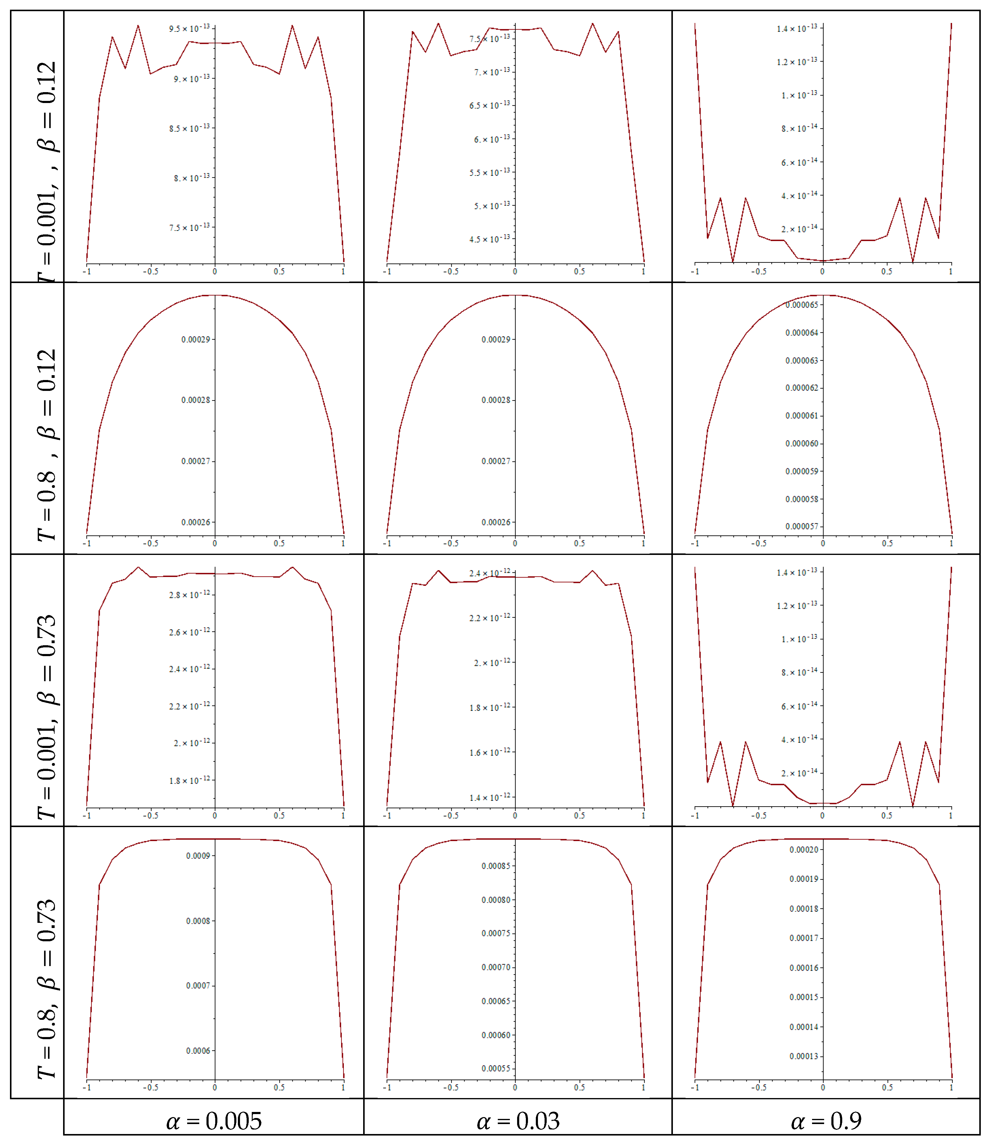
Table 1 and Table 2 include the exact solution, numerical values, and related errors when the kernel takes a logarithmic type of a cubic function w(u) = u³. Also, Figure 1 shows the error graphically in six curves for the calculations made for time values of 0.001 and 0.8 with different values of the parameter α = 0.005, 0.03, and 0.9. When $t=0.001$, the highest error is of order 10⁻¹, whereas the lowest error obtained in Table 1 is of order 10⁻¹⁰.

Table 1. The exact solution, the numerical solution, and the estimate of error at $T=0.001$.

$\mathit{x}$	Exact	$\mathit{\alpha }=0.005$		$\mathit{\alpha }=0.03$		$\mathit{\alpha }=0.9$
		App.	Error	App.	Error	App.	Error
−1	4.28714 × 10−4	4.28714 × 10−4	5.7161 × 10−13	4.28714 × 10−4	2.2864 × 10−13	4.28714 × 10−4	1.4290 × 10−13
−0.6	1.54337 × 10−4	1.54337 × 10−4	8.1800 × 10−13	1.54337 × 10−4	6.2251 × 10−13	1.54337 × 10−4	3.8570 × 10−14
−0.2	1.71486 × 10−5	1.71486 × 10−5	8.2813 × 10−13	1.71486 × 10−5	6.7637 × 10−13	1.71486 × 10−5	2.2860 × 10−15
0.2	1.71486 × 10−5	1.71486 × 10−5	8.2813 × 10−13	1.71486 × 10−5	6.7637 × 10−13	1.71486 × 10−5	2.2860 × 10−15
0.6	1.54337 × 10−4	1.54337 × 10−4	8.1800 × 10−13	1.54337 × 10−4	6.2251 × 10−13	1.54337 × 10−4	3.8570 × 10−14
1	4.28714 × 10−4	4.28714 × 10−4	5.7161 × 10−13	4.28714 × 10−4	2.2864 × 10−13	4.28714 × 10−4	1.4290 × 10−13

Table 2. The exact solution, the numerical solution, and the estimate of error at $T=0.8$.

$\mathit{x}$	Exact	$\mathit{\alpha }=0.005$		$\mathit{\alpha }=0.03$		$\mathit{\alpha }=0.9$
		App.	Error	App.	Error	App.	Error
−1	0.206000	0.20611701	1.17014 × 10−4	0.20611244	1.12441 × 10−4	0.20602572	2.57231 × 10−5
−0.6	0.074160	0.07442870	2.68709 × 10−4	0.07441821	2.582061 × 10−4	0.07421907	5.90696 × 10−5
−0.2	8.240 × 10−3	8.50309 × 10−3	2.63098 × 10−4	8.49281 × 10−3	2.52815 × 10−4	8.2978 × 10−3	5.78363 × 10−5
0.2	8.240 × 10−3	8.50309 × 10−3	2.63098 × 10−4	8.49281 × 10−3	2.52815 × 10−4	8.2978 × 10−3	5.78363 × 10−5
0.6	0.074160	0.07442870	2.68709 × 10−4	0.07441821	2.582061 × 10−4	0.07421907	5.90696 × 10−5
1	0.206000	0.20611701	1.17014 × 10−4	0.20611244	1.12441 × 10−4	0.20602572	257231 × 10−5

Figure 1. The error according to the time $t$, the parameter $\alpha$, and a logarithmic kernel.

Example 2. (Carleman-cubic function)

$$\psi \left(u,t\right)-{\displaystyle \frac{\lambda }{\mathsf{\Gamma }\left(\alpha \right)}}{\int }_0^t{\int }_{-1}^1{\left(t-\tau \right)}^{\alpha -1}{\left|u^3-v^3\right|}^{-\beta }\psi \left(v,\tau \right){\tau }^{2}dvd\tau =F\left(u,t\right)$$

(37)

Following the same method as Example (1) by using the exact solution $\psi \left(u,t\right)={\displaystyle \frac{u^2\left(t^2+t+0.002\right)}{7}}$ and the free function $F\left(u,t\right)={\displaystyle \frac{1}{7}}\left(t^2+t+0.002\right)f^{*}\left(u\right)$ in Equation $\left(37\right),\mathrm{w}\mathrm{e}\mathrm{h}\mathrm{a}\mathrm{v}\mathrm{e}$

$$f\left(u\right)=u^2+{\displaystyle \frac{1}{3}}\left\{{\displaystyle \frac{1}{1-\beta }}\left[{\left|u^3-1\right|}^{1-\beta }-{\left|1+u^3\right|}^{1-\beta }\right]-{\displaystyle \frac{1}{\left(1-\beta \right)\left(2-\beta \right)}}\left[{\left|u^3-1\right|}^{2-\beta }-{\left|1+u^3\right|}^{2-\beta }\right]\right\}.$$

The above equation of $f^{*}\left(u\right),\mathrm{f}\mathrm{o}\mathrm{r}u\in (-\mathrm{1,1})$ is a bounded and a continuous function. Hence, the condition of normality of $F\left(u,t\right)={\displaystyle \frac{1}{7}}\left(t^2+t+0.002\right)f^{*}\left(u\right)\mathrm{i}\mathrm{n}{L.}_2(-\mathrm{1,1})\times C\left[0,T\right]$ is satisfied.

Furthermore, for the position kernel condition,

$${\left(9{\int }_{-1}^1{\int }_{-1}^1({\left|u^3-v^3\right|}^{-2\beta }{u}^2{v}^{2}dudv\right)}^{{\displaystyle \frac{1}{2}}}\le {\displaystyle \frac{1}{9}}{\int }_{-1}^1\left({\int }_{-1}^1{\left|u^3-v^3\right|}^{-\beta }d{u}^3\right)d{v}^3],$$

and after integrating we obtain

$${\left(9{\int }_{-1}^1{\int }_{-1}^1({\left|u^3-v^3\right|}^{-2\beta }{u}^2{v}^{2}dudv\right)}^{{\displaystyle \frac{1}{2}}}\le {\displaystyle \frac{2^{3-\beta }}{9\left(1-\beta \right)\left(2-\beta \right)}},0\le \beta <1.$$

It is clear that the condition (i) is satisfied.

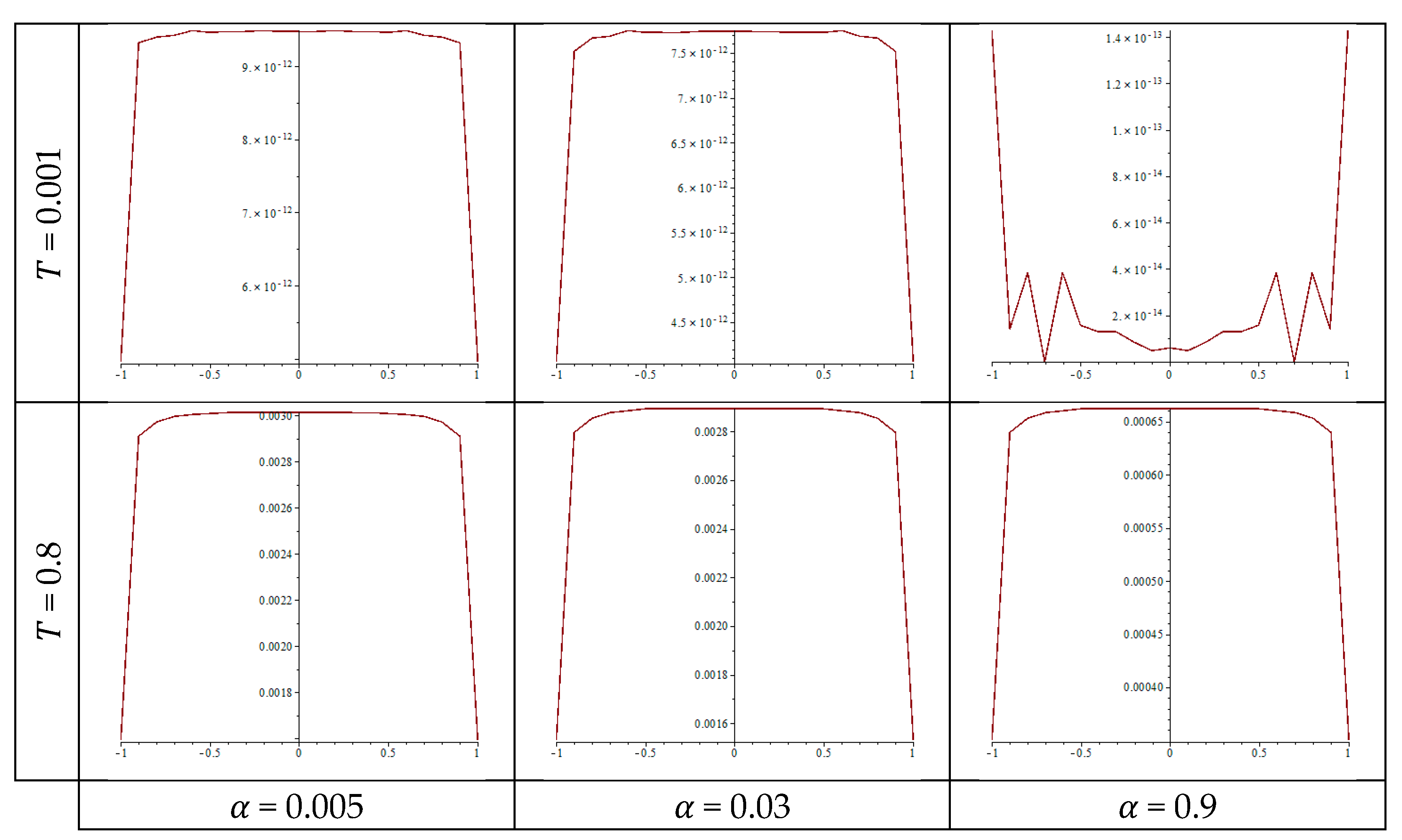
The computed values of the exact and approximate solutions, along with the associated errors, when the kernel takes the Carleman function, are shown in Table 3, Table 4, Table 5 and Table 6. For the fractional coefficient values $\alpha =0.005,0.03$ and $0.9att=0.001,t=0.8$, where the Carleman coefficient takes values $\beta =0.12$, and $0.73$. Figure 2 shows the error values graphically in 12 curves. It is seen that the largest error is of order 10⁻¹ at $t=0.8$ in Table 6, whilst the smallest error is of order 10⁻¹⁰ at $t=0.001$ in Table 3.

Table 3. The exact solution, numerical solution, and error estimate at $T=0.001,\beta =0.12$.

x	Exact	α = 0.005		α = 0.03		α = 0.9
		App.	Error	App.	Error	App.	Error
−1	4.28714 × 10−4	4.28714 × 10−4	7.1453 × 10−13	4.28714 × 10−4	4.1443 × 10−13	4.28714 × 10−4	1.4290 × 10−13
−0.6	1.54337 × 10−4	1.54337 × 10−4	9.5345 × 10−13	1.54337 × 10−4	7.7339 × 10−13	1.54337 × 10−4	3.8570 × 10−14
−0.2	1.71486 × 10−5	1.71486 × 10−5	9.3688 × 10−13	1.71486 × 10−5	7.6583 × 10−13	1.71486 × 10−5	2.2860 × 10−15
0.2	1.71486 × 10−5	1.71486 × 10−5	9.3688 × 10−13	1.71486 × 10−5	7.6583 × 10−13	1.71486 × 10−5	2.2860 × 10−15
0.6	1.54337 × 10−4	1.54337 × 10−4	9.5345 × 10−13	1.54337 × 10−4	7.7339 × 10−13	1.54337 × 10−4	3.8570 × 10−14
1	4.28714 × 10−4	4.28714 × 10−4	7.1453 × 10−13	4.28714 × 10−4	4.1443 × 10−13	4.28714 × 10−4	1.4290 × 10−13

Table 4. The exact solution, approximate solution, and error estimate at $T=0.8,\beta =0.12$.

x	Exact	α = 0.005		α = 0.03		α = 0.9
		App.	Error	App.	Error	App.	Error
−1	0.206000	0.20574196	2.58043 × 10−4	0.20575204	2.47959 × 10−4	0.20594327	5.67295 × 10−5
−0.6	0.074160	0.07386905	2.90953 × 10−4	0.07388042	2.79582 × 10−4	0.07409604	6.39646 × 10−5
−0.2	8.240 × 10−3	7.94335 × 10−3	2.96654 × 10−4	7.95494 × 10−3	2.85060 × 10−4	8.17478 × 10−3	6.52180 × 10−5
0.2	8.240 × 10−3	7.94335 × 10−3	2.96654 × 10−4	7.95494 × 10−3	2.85060 × 10−4	8.17478 × 10−3	6.52180 × 10−5
0.6	0.074160	0.07386905	2.90953 × 10−4	0.07388042	2.79582 × 10−4	0.07409604	6.39646 × 10−5
1	0.206000	0.20574196	2.58043 × 10−4	0.20575204	2.47959 × 10−4	0.20594327	5.67295 × 10−5

Table 5. The exact solution, numerical solution, and error estimate at $T=0.001,\beta =0.73$.

$\mathit{x}$	Exact	$\mathit{\alpha }=0.005$		$\mathit{\alpha }=0.03$		$\mathit{\alpha }=0.9$
		App.	Error	App.	Error	App.	Error
−1	4.28714 × 10−4	4.28714 × 10−4	1.6577 × 10−12	4.28714 × 10−4	1.3576 × 10−12	4.28714 × 10−4	1.4290 × 10−13
−0.6	1.54337 × 10−4	1.54337 × 10−4	2.9495 × 10−12	1.54337 × 10−4	2.4094 × 10−12	1.54337 × 10−4	3.8567 × 10−14
−0.2	1.71485 × 10−5	1.71485 × 10−5	2.9163 × 10−12	1.71486 × 10−5	2.3821 × 10−12	1.71486 × 10−5	5.2870 × 10−15
0.2	1.71485 × 10−5	1.71485 × 10−5	2.9163 × 10−12	1.71486 × 10−5	2.3821 × 10−12	1.71486 × 10−5	5.2870 × 10−15
0.6	1.54337 × 10−4	1.54337 × 10−4	2.9495 × 10−12	1.54337 × 10−4	2.4094 × 10−12	1.54337 × 10−4	3.8567 × 10−14
1	4.28714 × 10−4	4.28714 × 10−4	1.6577 × 10−12	4.28714 × 10−4	1.3576 × 10−12	4.28714 × 10−4	1.4290 × 10−13

Table 6. The exact solution, approximate solution, and error estimate at $T=0.8,\beta =0.73$.

x	Exact	$\mathit{\alpha }=0.005$		$\mathit{\alpha }=0.03$		$\mathit{\alpha }=0.9$
		App.	Error	App.	Error	App.	Error
−1	0.206000	0.20544240	5.57597 × 10−4	0.20546419	5.35807 × 10−4	0.20587741	1.22590 × 10−4
−0.6	0.074160	0.07324070	9.19298 × 10−4	0.07327663	8.83372 × 10−4	0.07395789	2.02111 × 10−4
−0.2	8.240 × 10−3	7.31460 × 10−3	9.25400 × 10−4	7.35076 × 10−3	8.89236 × 10−4	8.03655 × 10−3	2.03453 × 10−4
0.2	8.240 × 10−3	7.31460 × 10−3	9.25400 × 10−4	7.35076 × 10−3	8.89236 × 10−4	8.03655 × 10−3	2.03453 × 10−4
0.6	0.074160	0.07324070	9.19298 × 10−4	0.07327663	8.83372 × 10−4	0.07395789	2.02111 × 10−4
1	0.206000	0.20544240	5.57597 × 10−4	0.20546419	5.35807 × 10−4	0.20587741	1.22590 × 10−4

Figure 2. The error via the time $t$ and the parameters $\alpha ,\beta$, for the Carleman kernel.

Example 3. (Cauchy-cubic kernel)

$$\mu \psi \left(u,t\right)-{\displaystyle \frac{\lambda }{\mathsf{\Gamma }\left(\alpha \right)}}{\int }_0^t{\int }_{-1}^1{\displaystyle \frac{{\left(t-\tau \right)}^{\alpha -1}\psi \left(v,\tau \right){\tau }^2}{\left|u^3-v^3\right|}}dvd\tau =F\left(u,t\right).$$

(38)

According to the assumption of an exact solution and the time function $\psi \left(u,t\right)={\displaystyle \frac{u^2\left(t^2+t+0.002\right)}{7}}$, the free position function of the above function becomes

$$\begin{gathered} f^{*}\left(u\right)=u^2-2+u\left[{\displaystyle \frac{1}{3}}\mathrm{l}\mathrm{n}{\displaystyle \frac{\left|1-u\right|}{\left|1+u\right|}}-{\displaystyle \frac{1}{6}}\mathrm{l}\mathrm{n}{\displaystyle \frac{{\left(1+\frac{u}{2}\right)}^2+\frac{3u^2}{4}}{{\left(-1+\frac{u}{2}\right)}^2+\frac{3u^2}{4}}}\right] \\ +{\displaystyle \frac{u}{3\sqrt{3}}}\left(1+6u\right)\left[\mathrm{t}{\mathrm{a}\mathrm{n}}^{-1}\left(2{\displaystyle \frac{1+\frac{u}{2}}{\sqrt{3}u}}\right)-\mathrm{t}{\mathrm{a}\mathrm{n}}^{-1}\left(2{\displaystyle \frac{-1+\frac{u}{2}}{\sqrt{3}u}}\right)\right] \end{gathered}$$

From the above formula, we deduce that $f^{*}\left(u\right)\mathrm{i}\mathrm{s} \mathrm{b}\mathrm{o}\mathrm{u}\mathrm{n}\mathrm{d}\mathrm{e}\mathrm{d} \mathrm{a}\mathrm{n}\mathrm{d} \mathrm{c}\mathrm{o}\mathrm{n}\mathrm{t}\mathrm{i}\mathrm{n}\mathrm{u}\mathrm{o}\mathrm{u}\mathrm{s} \mathrm{f}\mathrm{o}\mathrm{r} u\in (-\mathrm{1,1}).$

Also, for the condition of position kernel, we have

$${\left(9\underset{-1}{\overset{1}{\int }}\underset{-1}{\overset{1}{\int }}{\displaystyle \frac{u^2{v}^2}{{\left|u^3-v^3\right|}^2}}dudv\right)}^{{\displaystyle \frac{1}{2}}}\le {\displaystyle \frac{1}{9}}{\int }_{-1}^1\left(\underset{-1}{\overset{1}{\int }}{\displaystyle \frac{d{u}^3}{\left|u^3-v^3\right|}}\right)d{v}^3]$$

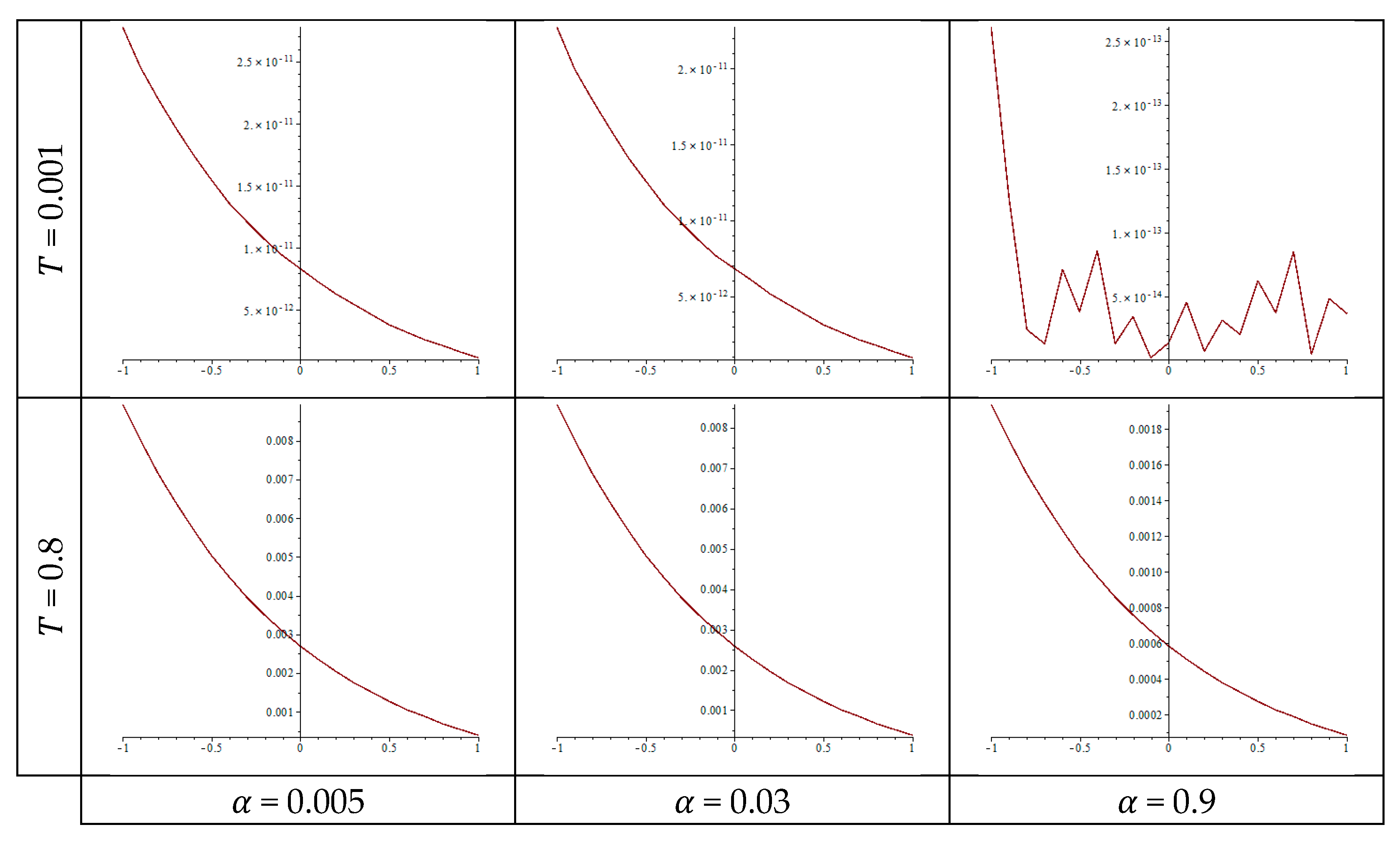
Hence, we have

$${\left(9\underset{-1}{\overset{1}{\int }}\underset{-1}{\overset{1}{\int }}{\displaystyle \frac{u^2{v}^2}{{\left|u^3-v^3\right|}^2}}dudv\right)}^{{\displaystyle \frac{1}{2}}}\le {\displaystyle \frac{4}{9}}\left(1+\mathrm{l}\mathrm{n}2\right)=\mathrm{f}\mathrm{i}\mathrm{n}\mathrm{i}\mathrm{t}\mathrm{e} \mathrm{t}\mathrm{e}\mathrm{r}\mathrm{m}$$

Table 7 and Table 8 indicate the calculated values of the exact and approximate solutions, as well as the corresponding errors, when the kernel takes the Cauchy kind. At $t=0.001, t=0.8$, the fractional coefficient values $\alpha =0.005, 0.03,$ and $0.9$ are used. The error curves are displayed in Figure 3. The highest inaccuracy in Table 8 is of order 10⁻¹ at t = 0.8, whereas the lowest error in Table 7 is of order 10⁻¹⁰ at $t=0.001$.

Table 7. The exact solution, the corresponding solution, and the estimate of error at $T=0.001$.

$\mathit{x}$	Exact	$\mathit{\alpha }=0.005$		$\mathit{\alpha }=0.03$		$\mathit{\alpha }=0.9$
		App.	Error	App.	Error	App.	Error
−1	4.28714 × 10−4	4.28714 × 10−4	4.9588 × 10−12	4.28714 × 10−4	4.0585 × 10−12	4.28714 × 10−4	1.4290 × 10−13
−0.6	1.54337 × 10−4	1.54337 × 10−4	9.4917 × 10−12	1.54337 × 10−4	7.7511 × 10−12	1.54337 × 10−4	3.8570 × 10−14
−0.2	1.71486 × 10−5	1.71486 × 10−5	9.4824 × 10−12	1.71486 × 10−5	7.7419 × 10−12	1.71486 × 10−5	8.2880 × 10−15
0.2	1.71486 × 10−5	1.71486 × 10−5	9.4824 × 10−12	1.71486 × 10−5	7.7419 × 10−12	1.71486 × 10−5	8.2880 × 10−15
0.6	1.54337 × 10−4	1.54337 × 10−4	9.4917 × 10−12	1.54337 × 10−4	7.7511 × 10−12	1.54337 × 10−4	3.8570 × 10−14
1	4.28714 × 10−4	4.28714 × 10−4	4.9588 × 10−12	4.28714 × 10−4	4.0585 × 10−12	4.28714 × 10−4	1.4290 × 10−13

Table 8. The exact solution, the approximate solution, and the estimate of error at $T=0.8$.

$\mathit{x}$	Exact	$\mathit{\alpha }=0.005$		$\mathit{\alpha }=0.03$		$\mathit{\alpha }=0.9$
		App.	Error	App.	Error	App.	Error
−1	0.206000	0.20440643	1.59357 × 10−3	0.2044687	1.53130 × 10−3	0.20564964	3.50357 × 10−4
−0.6	0.0741600	0.07115559	3.00441 × 10−3	0.0712730	2.88700 × 10−3	0.0734995	6.60537 × 10−4
−0.2	8.2400 × 10−3	5.22840 × 10−3	3.01159 × 10−4	5.34609 × 10−3	2.89390 × 10−4	7.57788 × 10−3	6.62117 × 10−5
0.2	8.2400 × 10−3	5.22840 × 10−3	3.01159 × 10−4	5.34609 × 10−3	2.89390 × 10−4	7.57788 × 10−3	6.62117 × 10−5
0.6	0.0741600	0.07115559	3.00441 × 10−3	0.0712730	2.88700 × 10−3	0.0734995	6.60537 × 10−4
1	0.206000	0.20440643	1.59357 × 10−3	0.2044687	1.53130 × 10−3	0.20564964	3.50357 × 10−4

Figure 3. The error according to the time $t$ and the parameter $\alpha ,$ with a Cauchy kernel.

Application 2:

In this application, $\omega \left(u\right)=e^{-u},$ and hence the kernel is expressed as $k\left(\left|\omega \left(u\right)-\omega \left(v\right)\right|\right)=k\left(\left|e^{-u}-e^{-v}\right|\right),$ with the exact solution $\psi \left(u,t\right)={\displaystyle \frac{e^{-u}\left(t^2+t+0.002\right)}{7}}.$

Example 4. (Logarithmic-exponential kernel)

$$\psi \left(u,t\right)-{\displaystyle \frac{\lambda }{\mathsf{\Gamma }\left(\alpha \right)}}{\int }_0^t{\int }_{-1}^1{\left(t-\tau \right)}^{\alpha -1}\ln \left|e^{-u}-e^{-v}\right|\psi \left(v,\tau \right){\mathrm{t}}^{2}dvd\tau =F\left(u,t\right).$$

(39)

Hence, the position term $f\left(u\right)$ takes the form

$$f^{*}\left(u\right)=e^{-u}-\left(e^{-1}-e^{-u}\right)\ln \left|e^{-1}-e^{-u}\right|+\left(e^1-e^{-u}\right)\ln \left|e^1-e^{-u}\right|+(e-e^{-1})$$

$f^{*}\left(u\right)$ is obviously bounded and continuous for $u\in (-1,1)$. Additionally, given condition (i), we perform the following

$${\left({\int }_{-1}^1{{\int }_{-1}^1(\ln \left|e^{-u}-e^{-v}\right|)}^2{e}^{-u}{e}^{-v}dudv\right)}^{{\displaystyle \frac{1}{2}}}\le {\int }_{-1}^1{\int }_{-1}^1\mathrm{l}\mathrm{n}\left|e^{-u}-e^{-v}\right|e^{-u}{e}^{-v}dudv$$

After integrating, we have

$${\left({\int }_{-1}^1{{\int }_{-1}^1(\ln \left|e^{-u}-e^{-v}\right|)}^2{e}^{-u}{e}^{-v}dudv\right)}^{{\displaystyle \frac{1}{2}}}\le 2(e-e^{-1})\ln \left|e-e^{-1}\right|-1+\left(e^2+e^{-2}\right)=\mathrm{f}\mathrm{i}\mathrm{n}\mathrm{i}\mathrm{t}\mathrm{e} \mathrm{n}\mathrm{u}\mathrm{m}\mathrm{b}\mathrm{e}\mathrm{r}$$

The exact solution, numerical values, and associated errors when the kernel takes a logarithmic type of an exponential function $w(u)=e^u$ are shown in Table 9 and Table 10. For calculations performed when the time takes the values 0.001 and 0.8 with various values of the parameter $\alpha =0.005,0.03$, and $0.9$. Figure 4 indicates the error for these cases in six curves. The lowest accuracy obtained in Table 10 is of order 10⁻² and the highest is of order 10⁻¹⁰ in Table 9.

Table 9. The exact solution, the numerical solution, and the error estimate at $T=0.001$.

$\mathit{x}$	Exact	$\mathit{\alpha }=0.005$		$\mathit{\alpha }=0.03$		$\mathit{\alpha }=0.9$
		App.	Error	App.	Error	App.	Error
−1	1.165366 × 10−3	1.16537 × 10−3	9.7984 × 10−12	1.16537 × 10−3	7.4677 × 10−12	1.16537 × 10−3	2.6114 × 10−13
−0.6	7.811684 × 10−4	7.81168 × 10−4	4.9584 × 10−12	7.81168 × 10−4	3.3960 × 10−12	7.81168 × 10−4	7.1429 × 10−14
−0.2	5.236328 × 10−4	5.23633 × 10−4	2.6037 × 10−12	5.23633 × 10−4	1.9851 × 10−12	5.23633 × 10−4	3.4571 × 10−14
0.2	3.510016 × 10−4	3.51002 × 10−4	1.3079 × 10−12	3.51002 × 10−4	9.4892 × 10−13	3.51002 × 10−4	7.5858 × 10−15
0.6	2.352834 × 10−4	2.35283 × 10−4	9.5485 × 10−13	2.35283 × 10−4	6.9864 × 10−13	2.35283 × 10−4	3.7700 × 10−14
1	1.577152 × 10−4	1.57715 × 10−4	1.0277 × 10−12	1.57715 × 10−4	7.9801 × 10−13	1.57715 × 10−4	3.6971 × 10−14

Table 10. The exact solution, the numerical solution, and the corresponding error at $T=0.8$.

$\mathit{x}$	Exact	$\mathit{\alpha }=0.005$		$\mathit{\alpha }=0.03$		$\mathit{\alpha }=0.9$
		App.	Error	App.	Error	App.	Error
−1	0.55996606	0.55685969	3.10637 × 10−3	0.5569804	2.98569 × 10−3	0.5592796	6.86411 × 10−4
−0.6	0.37535647	0.37392764	1.42883 × 10−3	0.3739832	1.37332 × 10−3	0.3750407	3.15727 × 10−4
−0.2	0.25160897	0.25088739	7.21581 × 10−4	0.2509154	6.93549 × 10−4	0.2514495	1.59447 × 10−4
0.2	0.16865854	0.16826433	3.94203 × 10−4	0.1682796	3.78889 × 10−4	0.1685714	8.71066 × 10−5
0.6	0.11305519	0.11278324	2.71960 × 10−4	0.1127938	2.61394 × 10−4	0.1129951	6.00946 × 10−5
1	0.07578316	0.07547805	3.05112 × 10−4	0.0754899	2.93259 × 10−4	0.0757157	6.74202 × 10−5

Figure 4. The error over the time $t$ and the parameter $\alpha ,$ with a log-exponential kernel.

Example 5. (Cauchy-exponential kernel)

$$\mu \psi \left(u,t\right)-{\displaystyle \frac{\lambda }{\mathsf{\Gamma }\left(\alpha \right)}}{\int }_0^t{\int }_{-1}^1{\left(t-\tau \right)}^{\alpha -1}/\left(e^{-u}-e^{-v}\right)\psi \left(v,\tau \right)t^{2}dvd\tau =F\left(u,t\right),$$

(40)

$$\left(\mathrm{T}\mathrm{h}\mathrm{e} \mathrm{e}\mathrm{x}\mathrm{a}\mathrm{c}\mathrm{t} \mathrm{s}\mathrm{o}\mathrm{l}\mathrm{u}\mathrm{t}\mathrm{i}\mathrm{o}\mathrm{n} \mathrm{i}\mathrm{s}\psi \left(u,t\right)={\displaystyle \frac{e^{-u}\left(t^2+t+0.002\right)}{7}}\right).$$

After separating the variables, we have $f^{*}\left(u\right)=\mu e^{-u}+\mathrm{l}\mathrm{n}[(e^{-u}-e^{-1}$)/$(e^{-u}-e^1$)}, where $f^{*}\left(u\right)$ is bounded and continuous at −1 < u < 1

For the condition of position kernel

$$\begin{gathered} {\left({\int }_{-1}^1{{\int }_{-1}^1(e^{-u}-e^{-v})}^{-2}{e}^{-u}{e}^{-v}dudv\right)}^{{\displaystyle \frac{1}{2}}}\le {\int }_{-1}^1{\int }_{-1}^1{\displaystyle \frac{e^{-u}{e}^{-v}dudv}{e^{-u}-e^{-v}}} \\ \le 4c\mathrm{o}\mathrm{s}\mathrm{h}e.\mathrm{l}\mathrm{n}2.\mathrm{c}\mathrm{o}\mathrm{s}\mathrm{h}2+4\mathrm{c}\mathrm{o}\mathrm{s}\mathrm{h}e\le \mathrm{c}\mathrm{o}\mathrm{n}\mathrm{s}\mathrm{t}\mathrm{a}\mathrm{n}\mathrm{t}. \end{gathered}$$

Table 11 and Table 12 indicate the calculated values of the exact and approximate solutions, as well as the corresponding errors, when the kernel takes the Cauchy kind as a function of an exponential function $w(u)=e^u$. The fractional coefficient values are $\alpha =0.005, 0.03,$ and $0.9$ at $t=0.001, t=0.8$. The error values are shown graphically in 6 curves in Figure 5. The maximum error is of order 10⁻² at $t=0.8$ in Table 12, while the minimum error in Table 11 is of order 10⁻¹⁰ at $t=0.001$.

Table 11. The exact solution, the numerical solution, and the error estimate at $T=0.001$.

$\mathit{x}$	Exact	$\mathit{\alpha }=0.005$		$\mathit{\alpha }=0.03$		$\mathit{\alpha }=0.9$
		App.	Error	App.	Error	App.	Error
−1	1.165366 × 10−3	1.16537 × 10−3	2.7793 × 10−11	1.16537 × 10−3	2.2744 × 10−11	1.16537 × 10−3	2.6114 × 10−13
−0.6	7.811684 × 10−4	7.81168 × 10−4	1.7394 × 10−11	7.81168 × 10−4	1.4151 × 10−11	7.81168 × 10−4	7.1428 × 10−14
−0.2	5.236328 × 10−4	5.23633 × 10−4	1.0684 × 10−11	5.23633 × 10−4	8.6512 × 10−12	5.23633 × 10−4	3.4571 × 10−14
0.2	3.510016 × 10−4	3.51002 × 10−4	6.2886 × 10−12	3.51002 × 10−4	5.1533 × 10−12	3.51002 × 10−4	7.5858 × 10−15
0.6	2.352834 × 10−4	2.35283 × 10−4	3.2115 × 10−12	2.35283 × 10−4	2.6200 × 10−12	2.35283 × 10−4	3.7700 × 10−14
1	1.577152 × 10−4	1.57715 × 10−4	1.1799 × 10−12	1.57715 × 10−4	9.5310 × 10−13	1.57715 × 10−4	3.6971 × 10−14

Table 12. The exact solution, the numerical solution, and the error at $T=0.8$.

$\mathit{x}$	Exact	$\mathit{\alpha }=0.005$		$\mathit{\alpha }=0.03$		$\mathit{\alpha }=0.9$
		App.	Error	App.	Error	App.	Error
−1	0.55996606	0.56890287	8.93682 × 10−3	0.56854784	8.58178 × 10−3	0.5619052	1.93917 × 10−3
−0.6	0.37535647	0.38103759	5.68111 × 10−3	0.3808119	5.45542 × 10−3	0.3765892	1.23273 × 10−3
−0.2	0.25160897	0.25510772	3.49875 × 10−3	0.2549687	3.35975 × 10−3	0.2523682	7.59182 × 10−4
0.2	0.16865854	0.17069440	2.03587 × 10−3	0.1706135	1.95498 × 10−3	0.1691003	4.41756 × 10−4
0.6	0.11305519	0.11411046	1.05527 × 10−3	0.1140685	1.01334 × 10−3	0.1132842	2.28979 × 10−4
1	0.07578316	0.07618112	3.97950 × 10−4	0.0761653	3.82141 × 10−4	0.0758695	8.63499 × 10−5

Figure 5. The error according to the time $t$ and the parameter $\alpha ,$ for a Cauchy-exponential kernel.

9. Discussion

Regarding the results given in the prior tables, we notice the following:

• In all previous cases, the numerical solutions obtained were very close to the exact solution.
• If time is fixed, the higher value of α, the smaller error.
• As the time values increase, the error increases for any fixed values of α.
• For the Carleman kernel, the error increased with decreasing values of $\beta$.
• It is evident how the symmetry of $u^2$ accounts for the symmetry in the results for generalized kernels in application (1).
• Because of the respective qualities of the functions, the error in the findings for $w\left(u\right)=u^3$ is more affected by time than its equivalent with $w\left(u\right)=e^{-u}$.
• It is obvious that the TMM is effective in solving this article’s issue.

10. Conclusions

In this study, we investigated the solution of an I-FrDE, under an initial condition with different forms of generalized symmetric singular kernels $k(\left|\omega (u)-\omega (v)\right|);u,v\in [-\mathrm{1,1}].$ The main goal is to accurately approximate the solution of the MIE which transformed from I-FrDE by applying the Riemann-Liouville fractional integral. A unique solution to MIE has been demonstrated using Picard’s method. To solve the MIE, we used the separation of variables method and then solved the obtained Fredholm integral equation by the TMM. The existence of a unique solution of the linear algebraic system in the Banach space ${\mathcal{l}}^{\mathrm{\infty }}$ has been proven. Many applications have been solved and their results calculated, which achieved high accuracy. All numerical results were computed using Maple18 software. The presented work opens doors to deal with more complex problems in real analysis and numerical computation fields.

References

- Tarasov, V.E. Fractional integro-differential equations for electromagnetic waves in dielectric media. Theor. Math. Phys. 2009, 158, 355–359. [Google Scholar] [CrossRef]
- Murugesan, M.; Shanmugam, S.; Rhaima, M.; Ravi, R. Analysis of Non-Local Integro-Differential Equations with Hadamard Fractional Derivatives: Existence, Uniqueness, and Stability in the Context of RLC Models. Fractal Fract. 2024, 8, 409. [Google Scholar] [CrossRef]
- Hao, Y.; Li, Q. Existence of Solutions for Fractional Integro-differential Equations with Impulsive and Integral Conditions. J. Nonlinear Model. Anal. 2019, 1, 221–235. [Google Scholar]
- Verma, P.; Kumar, M. An analytical solution with existence and uniqueness conditions for fractional integro-differential equations. Int. J. Model. Simul. Sci. Comput. 2020, 11, 2050045. [Google Scholar] [CrossRef]
- Abbas, M.I. Existence and uniqueness of mittage-leffler-ulam stable solution for fractional integrodifferential equations with nonlocal initial conditions. Eur. J. Pure Appl. Math. 2015, 8, 478–498. [Google Scholar]
- Wang, Y.; Zhu, L.; Wang, Z. Fractional-order Euler functions for solving fractional integro-differential equations with weakly singular kernel. Adv. Differ. Equ. 2018, 2018, 1–13. [Google Scholar] [CrossRef]
- Li, M.; Wang, L.; Liu, Y. Generalized hat functions method for solving fractional integro-differential equations of bratu-type. IAENG Int. J. Comput. Sci. 2017, 44, 105–111. [Google Scholar]
- Raad, S.; Alqurashi, K. Toeplitz matrix and Nyström method for solving linear fractional integro-differential equation. Eur. J. Pure Appl. Math. 2022, 15, 796–809. [Google Scholar] [CrossRef]
- Alkan, S.; Hatipoglu, V.F. Approximate solutions of Volterra-Fredholm integro-differential equations of fractional order. Tbilisi Math. J. 2017, 10, 1–13. [Google Scholar] [CrossRef]
- Li, J.; Zhao, K.; Su, X. Barycentric Interpolation Collocation Method for Solving Fractional Linear Fredholm-Volterra Integro-Differential Equation. J. Funct. Spaces 2023, 1, 7918713. [Google Scholar] [CrossRef]
- Devi, J.V.; Sreedhar, C.V. Generalized monotone iterative method for Caputo fractional integro-differential equation. Eur. J. Pure Appl. Math. 2016, 9, 346–359. [Google Scholar]
- Mahdy, A.M.; Abdou, M.A.; Mohamed, D.S. Computational methods for solving higher-order (1 + 1) dimensional mixed-difference integro-differential equations with variable coefficients. Mathematics 2023, 11, 2045. [Google Scholar] [CrossRef]
- Alhazmi, S.E.; Abdou, M.A.; Basseem, M. Physical phenomena of spectral relationships via quadratic third kind mixed integral equation with discontinuous kernel. AIMS Math. 2023, 8, 24379–24400. [Google Scholar] [CrossRef]
- Jan, A.R. An asymptotic model for solving mixed integral equation in position and time. J. Math. 2022, 2022, 8063971. [Google Scholar] [CrossRef]
- Jebreen, H.B. On the Multiwavelets Galerkin Solution of the Volterra–Fredholm Integral Equations by an Efficient Algorithm. J. Math. 2020, 2020, 2672683. [Google Scholar] [CrossRef]
- Micula, S. On some iterative numerical methods for mixed Volterra–Fredholm integral equations. Symmetry 2019, 11, 1200. [Google Scholar] [CrossRef]
- Geçmen, M.Z.; Çelik, E. Numerical solution of Volterra–Fredholm integral equations with Hosoya polynomials. Math. Methods Appl. Sci. 2021, 44, 11166–11173. [Google Scholar] [CrossRef]
- Esmaeili, H.; Rostami, M.; Hooshyarbakhsh, V. Numerical solution of Volterra-Fredholm integral equation via hyperbolic basis functions. Int. J. Numer. Model. Electron. Netw. Devices Fields 2021, 34, e2823. [Google Scholar] [CrossRef]
- WANG, Y.; ZHOU, X. An Efficient Numerical Method Based on Bell Wavelets for Solving the Fractional Integro-Differential Equations with Weakly Singular Kernels. Fractal Fract. 2024, 8, 74. [Google Scholar] [CrossRef]
- Abdou, M.A.; El-Kojok, M.M.; Raad, S.A. On the solution of Fredholm-Volterra integral equation with discontinuous kernel in time. J. Adv. Math. 2014, 9, 2553–2563. [Google Scholar]
Disclaimer/Publisher’s Note: The statements, opinions and data contained in all publications are solely those of the individual author(s) and contributor(s) and not of MDPI and/or the editor(s). MDPI and/or the editor(s) disclaim responsibility for any injury to people or property resulting from any ideas, methods, instructions or products referred to in the content. |
© 2024 by the authors. Licensee MDPI, Basel, Switzerland. This article is an open access article distributed under the terms and conditions of the Creative Commons Attribution (CC BY) license (https://creativecommons.org/licenses/by/4.0/).