Abstract
Ebola virus disease (EVD) is a severe and often fatal illness posing significant public health challenges. This study investigates EVD transmission dynamics using a novel fractional mathematical model with five distinct compartments: individuals with low susceptibility (), individuals with high susceptibility (), infected individuals (), exposed individuals (), and recovered individuals (). To capture the complex dynamics of EVD, we employ a -piecewise hybrid fractional derivative approach. We investigate the crossover effect and its impact on disease dynamics by dividing the study interval into two subintervals and utilize the -Caputo derivative in the first interval and the -ABC derivative in the second interval. The study determines the basic reproduction number , analyzes the stability of the disease-free equilibrium and investigates the sensitivity of the parameters to understand how variations affect the system’s behavior and outcomes. Numerical simulations support the model and demonstrate consistent results with the theoretical analysis, highlighting the importance of fractional calculus in modeling infectious diseases. This research provides valuable information for developing effective control strategies to combat EVD.
1. Introduction
Ebola virus disease (EVD) is a severe, often fatal illness primarily affecting humans and primates, which is caused by the Ebola virus. It leads to hemorrhagic fever and spreads through direct contact with infected bodily fluids. While EVD outbreaks have occurred sporadically in sub-Saharan Africa [1] since its discovery in 1976, the largest outbreak to date ravaged West Africa between 2013 and 2016, claiming over 11,000 lives [2,3,4]. Subsequent outbreaks in the Democratic Republic of the Congo in 2017, 2018 [5,6], and 2019 [7,8] were also severe, highlighting the ongoing challenge this deadly virus poses [9]. Fatality rates range from 25% to 90% with death often occurring within two weeks. The early diagnosis of EVD is challenging due to its initial symptoms resembling many common African diseases, including malaria, dengue fever, and other hemorrhagic fevers [10,11,12]. While no cure exists for EVD, early supportive treatment, including oral and intravenous rehydration, is crucial. An FDA-approved vaccine and treatments like Inmazeb offer hope [13], while prevention efforts focus on hygiene, the safe handling of bushmeat, and rapid response to outbreaks, including contact tracing and the proper disposal of deceased individuals.
Mathematical models play a vital role in simulating the transmission dynamics of diseases, providing insights into the disease’s spread and potential intervention strategies. By simulating the transmission dynamics, these models can help predict future outbreaks, identify vulnerable populations, and evaluate the effectiveness of various control measures. This knowledge is essential for guiding public health interventions and prioritizing research efforts. The fight against Ebola is a complex and multifaceted endeavor, demanding a collaborative effort from governments, international organizations, scientists, and communities to mitigate future outbreaks and minimize the devastating consequences of this disease.
Fractional derivatives offer key advantages over classical ones by incorporating memory effects, capturing the crossover effect between transmission phases, and representing heterogeneity in susceptibility. These features allow for a more realistic and accurate representation of disease dynamics, leading to improved model fit, predictive capabilities, and insights for designing effective public health interventions.
Regarding Ebola virus disease (EVD), numerous studies have been published in the literature aimed at identifying EVD and exploring its potential eradication. For instance, Ahmad et al. [14] presented an innovative SVEIR model for analyzing Ebola spread, suggesting that voluntary vaccination could effectively control outbreaks. However, its reliance on simplifying assumptions and the need for accurate data may limit practical applicability and overlook sociocultural factors. Nazir et al. [15] studied the Ebola virus transmission model through an advanced conformable mathematical approach, improving accuracy and responsiveness for public health strategies, but its complexity and reliance on reliable data may limit practical applicability and generalizability to other diseases. Ahmad and Abbas [16] developed a susceptible–exposed–infected–quarantined–recovered model to analyze the impact of quarantine on Ebola virus transmission dynamics, highlighting that effective quarantine measures can significantly reduce disease spread and validating the findings through numerical methods. Yadav et al. [17] presented a fractional order mathematical model of the Ebola virus using the ABC operator, capturing memory effects in transmission dynamics and potentially improving accuracy in predicting epidemic trends and informing control strategies. Baller et al. [18] analyzed real data from the EVD outbreaks in the Democratic Republic of Congo during 2018 and 2020. The authors in [19] discuss a detailed analysis of a stochastic EVD model that incorporates multiple delays and is based on a probability density function. Optimal control modeling for EVD is examined in [20]. Additionally, the authors in [21] address EVD considering sexual transmission and the persistence of the Ebola virus in the male reproductive tract.
Recently, in 2021, Atangana-Seda [22] introduced a novel technique based on piecewise hybrid differential and integral operators, offering a fresh perspective and enhanced capabilities for modeling and solving complex real-world problems. This piecewise fractional operator offers remarkable flexibility in representing systems characterized by diverse dynamics. By accommodating distinct behaviors like growth, decay, or oscillations within separate regions or intervals, it facilitates a more nuanced and comprehensive understanding of the system’s evolution [23,24,25,26]. For example, the piecewise mathematical model for Nipah virus disease was studied by [27]. The model of Rubella disease using a piecewise hybrid fractional order was discussed in [28], while [29] discussed hepatitis B virus modeling through similar methods. An epidemic model for the Ebola virus using a piecewise hybrid fractional order was presented in [30], and optimal control strategies for Ebola were studied in [31].
This work enhances existing five-compartment fractional mathematical models of Ebola virus disease (EVD) [32] by employing a novel -piecewise hybrid fractional derivative approach [22]. We partition the study interval into two subintervals: and [33], applying the -Caputo fractional derivative in the first interval [34,35] and the -ABC fractional derivative in the second [36]. This partitioning allows us to investigate the crossover effect of the shift in model dynamics as we transition between fractional operators and their impact on EVD transmission patterns, particularly how variations in susceptibility influence these patterns over time.
Our comprehensive framework represents a significant advancement in EVD modeling by merging advanced mathematical techniques with a detailed compartmental structure, offering a more nuanced representation of disease progression than previous models. This enhanced compartmentalization, coupled with hybrid fractional derivatives, enables more accurate predictions of EVD transmission dynamics, informing more effective public health strategies for outbreak management and ultimately leading to improved disease control and reduced mortality.
Specifically, our work introduces two new concepts of fractional derivatives:
- -ABC and -Caputo fractional derivatives: These generalizations provide greater flexibility in modeling disease dynamics by incorporating the influence of various factors affecting transmission.
- -piecewise hybrid fractional derivative (-PCABC): This approach enables us to model the transition between different phases of an outbreak, where initial conditions and memory effects play varying roles, providing a more nuanced understanding of disease dynamics and improving the accuracy of model predictions.
- The choice of the -Caputo and -ABC operators is a key innovation of our manuscript, significantly advancing the application of fractional calculus in infectious disease modeling. This approach offers a fresh perspective and a new framework for applying fractional calculus to complex disease dynamics, substantially expanding the state of the literature.
This paper is structured as follows: Section 2 introduces the fundamental concepts of the ABC fractional operator, detailing its relationship with and introducing -PCABC. Rigorous definitions of piecewise hybrid fractional derivatives are provided in this context. Section 3 presents a mathematical model incorporating the -PCABC fractional order, highlighting the crossover behavior of the EVD model. Section 4 focuses on the qualitative analysis of the Ebola model, examining critical aspects such as the boundedness and positivity of solutions, the disease-free equilibrium point, the basic reproduction number, the stability of the disease-free equilibrium point, and a sensitivity analysis of the relevant parameters. Section 5 establishes the Lipschitz property and discusses the existence and uniqueness of the model solution. Section 6 establishes the solution of Ebola Model via Recursive Sequences. Section 7 introduces a numerical scheme utilizing -piecewise hybrid derivatives. Section 8 presents simulations and a thorough discussion of the results. Finally, the paper concludes by summarizing the findings and their implications.
2. Basic Concepts
This section establishes the foundation for our subsequent analysis by defining the key concepts of the ABC fractional derivative and piecewise hybrid fractional derivatives.
2.1. ABC Fractional Operator
Atangana and Baleanu [37] defined a fractional derivative with a non-local and non-singular kernel for a function of order as follows:
where is the normalization function, denotes the derivative of , and is the M-L function defined by
This derivative accounts for the influence of past events on the current state of the system, providing a more realistic representation of disease dynamics. The corresponding fractional integral of the ABC fractional derivative is given by [37]
where is the R-L-fractional integral of function of order defined by [38]
2.2. Piecewise Hybrid Fractional Derivatives
Atangana and Araz in 2021 [22] investigated new concepts of fractional derivatives called piecewise hybrid fractional derivatives. One from these derivatives is called a piecewise hybrid derivative with Caputo and M-L kernel that is defined by
where is the Caputo fractional derivative and is the ABC fractional derivative. The corresponding fractional integral is defined by
2.3. -ABC Fractional Operator
Building upon the ABC fractional derivative [37], the authors in [36] extended the definition to include a non-decreasing function for all as follows
where This generalization allows for greater flexibility in modeling disease dynamics, as it allows us to incorporate the influence of various factors that affect disease transmission. Also, the authors in [36] introduced the definition of an AB fractional integral with respect to as follows
where is the -R-L-fractional integral of function of order defined by [38]
2.4. -Piecewise Hybrid Fractional Derivative
Here, by the definition of the - fractional derivative defined in [36], and the definition of the -C fractional derivative defined in [35], we present the definitions of the -piecewise hybrid derivative and integral with -C and -. The -piecewise hybrid derivative with -C and -, denoted by (-), is given as
where is the -Caputo fractional derivative and is the - fractional derivative. This generalization allows for greater flexibility in modeling disease dynamics, as it allows us to incorporate the influence of various factors that affect disease transmission. The corresponding fractional integral is defined by
3. Mathematical Model
The proposed fractional model for Ebola meticulously dissects the total human population, denoted as , into five distinct and mutually exclusive compartments, offering a comprehensive framework for understanding the disease’s dynamics. The susceptible population, those at risk of contracting the virus, is further subdivided into two subclasses: individuals with a low risk of susceptibility, represented as , and individuals with a high risk of susceptibility, represented as . We divide the susceptible population into lower and higher risk groups based on evidence that the EVD susceptibility varies due to occupational exposure, age and health, genetics and prior exposure; see [32,39,40]. Additionally, the model incorporates compartments for exposed individuals , infected individuals , and recovered individuals . The sum of these compartments constitutes the total population, as expressed by the following equation:
The high-risk susceptible population, , encompasses individuals who are most vulnerable to contracting the virus from infected individuals. This category includes individuals involved in the burial process, healthcare workers, and relatives of infected individuals. The remaining segment of the population, denoted by , is classified as having a minimal likelihood of contracting the virus. Susceptible individuals are constantly introduced into the population through birth and immigration at a steady rate of . Of these new individuals, the proportion deemed to be at high risk of infection is represented by the parameter , while the remaining proportion () represents individuals with a low risk of infection.
The infection rate for the low-risk susceptible population is denoted as , whereas the infection rate for the high-risk population is . Here, is a class modification parameter that reflects the heightened susceptibility of the high-risk group. The parameter should be greater than 1. A natural mortality rate applies to all five compartments (except the infected compartment), which also experiences an additional mortality rate specifically due to the infection.
The exposed population increases as individuals from both susceptible populations, and , transition into this category through interactions with individuals who are already infected. The rates of infection for these two populations are denoted as and , respectively. Exposed individuals transition to the infected class at a rate denoted as as they begin to exhibit symptoms. The size of the infected class increases as exposed individuals transition to the symptomatic stage with a growth rate represented by . The infected class decreases due to mortality (natural deaths at a rate and disease-induced deaths at a rate ) or recovery from the infection, which occurs at a rate denoted by .
This detailed compartmental structure of the model allows for a more nuanced and realistic representation of the Ebola virus disease’s spread and its impact on the population. It is crucial to inform effective public health interventions and control strategies.
Here, we extend the Ebola model presented in [32] by incorporating the -piecewise hybrid fractional derivative approach. The --fractional model, expressed in terms of fractional state variables, and with a derivative order of , can be formulated in the following conventional form:
The model is subject to the following initial conditions: , , , , and . The schematic diagram of our proposed model is given in Figure 1.
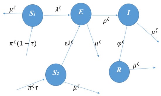
Figure 1.
Schematic diagram of our proposed model.
Advantages of -Piecewise Hybrid Fractional Derivative
The -piecewise hybrid fractional derivative used in this work is a novel approach that combines two different types of fractional derivatives (-Caputo and -ABC) within a single model applied over distinct intervals of the independent variable (usually time). This approach allows us to effectively capture the crossover effect observed in many real-world outbreaks.
In the beginning, we divide the study interval into two subintervals: and . In the early phase of an Ebola outbreak, represented by the interval , we know that the primary transmission mechanism is direct contact with infected individuals. The -Caputo derivative, which emphasizes the local behavior of the system, is well suited to model this initial stage, where the immediate impact of infected individuals on susceptible populations is most pronounced. This phase is characterized by rapid spread driven primarily by direct contact and the absence of substantial acquired immunity or widespread public health interventions.
As the outbreak progresses, represented by the interval , the dynamics become more complex. The influence of factors beyond immediate contacts, such as acquired immunity, public health interventions, behavioral changes, and environmental factors, becomes increasingly significant. In this phase, the -ABC fractional derivative, which incorporates memory effects, is better suited to model this later phase where the outbreak’s history and the cumulative impact of these factors are crucial. It allows us to represent the system’s memory, capturing the influence of past events on the present state, which is essential for accurately modeling the evolving outbreak dynamics.
The point represents a transition point where the dominant mechanism shifts from localized direct transmission to a more complex, memory-dependent dynamic, leading to the observed crossover effect. The choice of is based on the assumption that this transition occurs at a specific point in the outbreak.
Also, the function in our model allows for a more flexible representation of the transition dynamics. The choice of is informed by the assumption that the rate of change in the dominant transmission mechanism is not constant throughout the outbreak.
4. Crossover Behavior
To analyze the crossover behavior and capture the evolving dynamics of Ebola transmission, we partition our model (1) into two phases:
- Early Phase (): Characterized by localized direct transmission as the dominant mechanism.
- Later Phase (): Where memory effects, such as acquired immunity and interventions, become increasingly influential.
This partitioning allows us to investigate the crossover point at which the dominant transmission mechanism shifts and to accurately represent the changing influence of various factors over time. Using this approach, model (1) can be rewritten as follows:
and
where and represent the Caputo and ABC derivatives with respect to the function , respectively.
5. Qualitative Analysis of the Ebola Model (1)
This section delves into the fundamental properties of the Ebola model presented in Equation (1). Specifically, we will investigate the boundedness and positivity of the model’s solutions, analyze the disease-free equilibrium point and its stability, and calculate the basic reproduction number . We will also examine the sensitivity of the model’s parameters to determine which factors have the most significant influence on the spread of Ebola.
5.1. Boundedness of the Solutions
Theorem 1.
The solution set of the Φ-piecewise hybrid Ebola model (1) is bounded within the biologically and mathematically feasible region where
Proof.
To ensure the biological feasibility of our model, we need to demonstrate that the population size remains bounded. In our model, the -piecewise hybrid derivative of the total population, , at time z represents
where
Clearly
This implies that
By definition , the inequality (2) becomes
Now, for , we have
We apply the Laplace transform with respect to function on both sides of (3) and obtain
Thus, according to the Laplace transform of Caputo fractional derivative with respect to function defined in [41,42], we obtain
Consequently, is bounded by in case
Next, for , we have
We apply the Laplace transform with respect to function on both sides of (4) and obtain
Using the definition of the Laplace transform for the derivative (as detailed in [43]) and leveraging the asymptotic behavior of the M-L function (as described in [44,45]), we can show that the total population size is bounded by in . Therefore, by considering both subintervals, we conclude that the total population size is bounded by in . Since , we can conclude that all state variables are bounded in region , ensuring the biological feasibility of the model. □
5.2. Positivity of the Solutions
Theorem 2.
Model (1), with initial conditions , and , guarantees positive solutions for all time.
Proof.
To ensure the biological relevance of our model, we need to demonstrate that all state variables remain non-negative. We will prove this by showing that each state variable remains positive for all time . To analyze this, we examine the third equation of model (1), which takes the following form:
Then, we have
By the definition of the fractional derivative, the inequality (5) becomes
Now, for , we have
By same technique using in [41,42], we have
This demonstrates that the solution remains positive for all values of z within the interval .
Next, for , we have
The Laplace transform with respect to of both sides of (6) yields
Thus, we obtain
Upon applying the inverse Laplace transform with respect to , we obtain the following solution
Given and the fact that , we deduce that remains positive for all . Combining this with the previous analysis for the interval , we can definitively state that is a positive solution for all . Applying the same manner, we can demonstrate that and are positive, ensuring the model’s biological feasibility. □
5.3. Disease-Free Equilibrium Point (DFEP)
5.4. Basic Reproduction Number
To obtain the basic reproduction number , we consider the exposed and infected classes as the following equations:
Thus, this system can be written as
where
and
The Jacobian matrices of functions and at are given by
and
Using , the basic reproduction number for model (1) is
5.5. Stability of the Disease-Free Equilibrium Point
The stability of the disease-free equilibrium point is a fundamental concept in infectious disease modeling because it tells us whether a disease is likely to persist in a population or eventually disappear. A stable disease-free equilibrium indicates that even if a few infected individuals are introduced, the disease will die out naturally due to insufficient transmission. However, an unstable disease-free equilibrium signifies that even a small introduction of the disease could lead to a sustained outbreak. This crucial information guides the development of control strategies, allowing us to target interventions that either maintain a stable disease-free equilibrium or shift an unstable one toward stability. By understanding the factors that influence the stability of the disease-free equilibrium, we can identify key drivers of transmission and tailor control measures to effectively protect public health.
Theorem 3.
The disease-free equilibrium of the model (1) is locally stable if and unstable if
Proof.
By the same analysis of stability in the Ebola model [32], we conclude that when , the disease-free equilibrium is locally stable, indicating that any small outbreak will eventually die out. However, if , the disease-free equilibrium becomes unstable, suggesting that even a small introduction of the disease can lead to a sustained epidemic. □
5.6. Sensitivity Analysis
This subsection applies sensitivity analysis methods to calculate the basic reproduction number and the sensitivity indices for the model’s parameters. These indices highlight the significance of each factor in disease emergence and transmission. Sensitivity analysis also assesses how resilient the model’s predictions are to changes in parameter values. To calculate the sensitivity indices, we utilize the following formula:
Applying the above formula gives
Figure 2 presents an overview of sensitivity indices for the parameters of the model.
From the above analysis, we conclude the following:
- The most influential parameters for increasing : , , and (positive elasticity).
- Parameters that decrease : , and (negative elasticity).
- Strongest influence: has a stronger positive influence than , despite both being positive.
- Practical implications: Target interventions to reduce parameters with high positive elasticity for maximum impact on controlling outbreaks.
- Efforts to improve recovery rates will have a limited impact on due to its low elasticity.
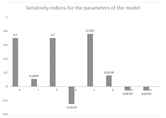
Figure 2.
Overview of sensitivity indices used in calculating .
5.7. Existence and Uniqueness of Solution via Fixed Point Theorem
This subsection focuses on examining the existence and uniqueness of a solution for the model (1) through the application of the fixed point technique. Let then, we define the Banach space under the norm
where In the following analysis, we use the compact initial value problem defined as
where
and
Define an operator as
Theorem 4
(Existence). Assume that the function is continuous such that
Then, the model (1) has a solution, provided that
Proof.
Let us consider the operator defined by (10). To establish the existence of a solution for the model (1), it suffices to demonstrate that the operator has a fixed point. For this purpose, we define the closed ball as follows:
with
We will divide the proof into several steps as outlined below:
Step (1).
This proves that
Step (2). The operator is relatively compact, meaning it is continuous, uniformly bounded, and equicontinuous.
The continuity of the function indicates that the operator is also continuous. Let Then, the inequality (11) provides the following:
Hence, is uniformly bounded on . Let Then, we have
It can be concluded that
This implies that . Therefore, is equicontinuous and compact on according to the Arzelá–Ascoli theorem. Consequently, by the Leray–Schauder theorem, the model (1) possesses at least one solution. □
Theorem 5
(Uniqueness). Assume that the function is continuous such that
Then, the model (1) has a unique solution, provided that
6. Solution of Model (1) via Recursive Sequences
Make use of the integral operator in - on the Ebola model (1); then, we shall have
and
where and are the kernels defined as follows
6.1. Lipschitz Property
Theorem 6.
Given that are continuous functions in , we can find positive constants , and such that
Then, the kernels and defined by (13) satisfy Lipschitz conditions with Lipschitz constant , such that
Proof.
For let Then,
Put Thus, we obtain
To further demonstrate the concept, we can obtain the following:
and
Let
This shows that the function is Lipschitz continuous with a Lipschitz constant □
6.2. Existence of Solution via Recursive Sequences
Theorem 7.
Assuming that the kernels satisfy the Lipschitz condition with Lipschitz constant (as established in Theorem ), and if
then model (1) has a solution.
Proof.
To solve the model numerically, we introduce the following recursive formulas:
For our subsequent analysis, we define the functions () as follows:
By applying the norm to the system of equations above, we obtain
By Theorem 6, we have
Thus, (15) becomes
Given that
we observe that converges to zero as n approaches infinity. Applying similar reasoning, we can conclude that
and
Based on the inequalities obtained above, and inequality (14), we can conclude that
Consequently, we can conclude that model (1) has a solution. □
7. Numerical Scheme with -Piecewise Hybrid Derivative
In this section, we employ a numerical scheme based on the concept of the -piecewise hybrid Caputo and Atangana–Baleanu fractional integral to solve the fractional-order Ebola model. This scheme is specifically designed to handle the complexities introduced by the piecewise hybrid fractional derivative approach. The fractional derivatives and integrals were approximated using numerical integration techniques. We utilized the Trapezoidal and Adams–Bashforth–Moulton methods adapted for fractional operators, which offer a balance of accuracy and computational efficiency [22]. By applying the -piecewise hybrid Caputo and Atangana–Baleanu fractional integral, we have
and
Now, put , we obtain
and
Convergence of the Scheme
We provide a theorem (Theorem 7 in this paper) that establishes conditions under which the proposed numerical scheme has a solution, implying its convergence. However, the scheme does not converge unconditionally. The convergence of our scheme depends on several factors:
- Lipschitz Condition: The kernels (interaction terms) in the model must satisfy the Lipschitz condition.
- Convergence Condition: An inequality involving the Lipschitz constant, fractional order, increasing function , and interval lengths must be satisfied (detailed in Theorem 7).
8. Simulations and Discussion
This section provides a graphical interpretation of the -piecewise hybrid fractional Ebola model (1). We investigate the model’s behavior for various values of the fractional order and a suitable increasing function . By visualizing the model’s dynamics, we gain a deeper understanding of how fractional derivatives and the choice of influence the spread of Ebola. The parameter values used in our numerical simulations were carefully chosen based on a combination of a literature review [32,46,47], real-world data from previous outbreaks, and expert consultation. These parameters have practical biological significance, reflecting key aspects of EVD transmission and progression. Our sensitivity analysis provides insights into the robustness of our results and highlights areas where further research is needed to reduce parameter uncertainty. Here, we will use the relevant biological parameters , , with the following initial values
Figure 3, Figure 4, Figure 5, Figure 6, Figure 7, Figure 8, Figure 9, Figure 10, Figure 11 and Figure 12 illustrate the numerical solutions of the proposed -piecewise hybrid fractional Ebola model, showcasing the population dynamics within each of the five compartments (, , , , ) over time. The simulations highlight the impact of varying the fractional order and the increasing function on the model’s behavior. We present graphical illustrations for two cases as follows.
8.1. Case-I:
Figure 3, Figure 4, Figure 5, Figure 6 and Figure 7 depict the solutions graphically for fractional orders ranging from , and with . The crossover effect is evident near .
Figure 3 (Susceptible Population ): The low-risk susceptible population exhibits a consistent decrease over time as individuals transition to the exposed and infected classes. Smaller fractional orders result in a more rapid decrease, signifying faster disease spread.
Figure 4 (High-Risk Susceptible Population ): The high-risk susceptible population shows a consistent decrease over time for all fractional orders.
Figure 5 (Exposed Population ): The exposed population shows a rapid initial increase, peaking earlier and more prominently for smaller fractional orders. This highlights the quicker initial spread associated with lower values. The crossover effect, the gradual transition from -Caputo to -ABC derivative, is observed as a gradual increase in the exposed class over time rather than a sudden “bump” near .
Figure 6 (Infected Population ): The infected population initially decreases due to recoveries and deaths, which is followed by a gradual increase and eventual stabilization. This pattern aligns with the crossover effect observed in the exposed population. Smaller values lead to a more rapid initial decrease and a sharper rise, highlighting the influence of memory effects on disease transmission.
Figure 7 (Recovered Population ): The recovered population exhibits a gradual increase as infected individuals recover, which is followed by a slight decline and eventual stabilization. The peak is higher for smaller values, suggesting a larger proportion of recovered individuals with faster initial spread.
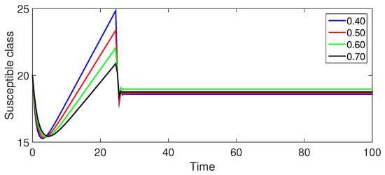
Figure 3.
Numerical illustration for susceptible class at fractional orders ranging from , and with .
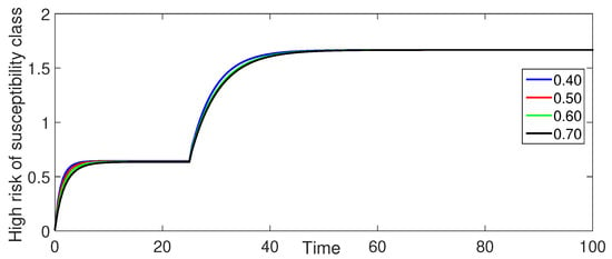
Figure 4.
Numerical illustration for high risk of susceptibility class at fractional orders ranging from and with .
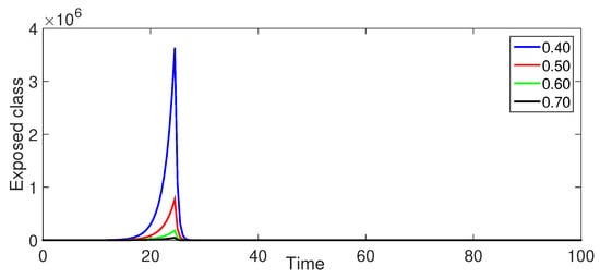
Figure 5.
Numerical illustration for exposed class at fractional orders ranging from , and with .
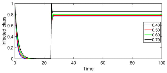
Figure 6.
Numerical illustration for infected class at fractional orders ranging from , and with .
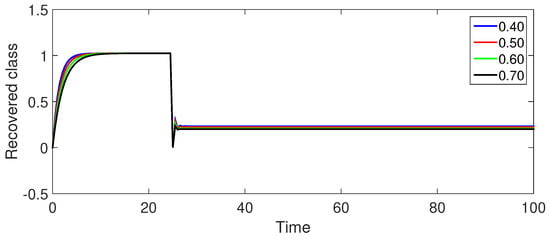
Figure 7.
Numerical illustration for recovered class at fractional orders ranging from , and with .
8.2. Case-II:
Figure 8, Figure 9, Figure 10, Figure 11 and Figure 12 illustrate the solutions graphically for fractional orders ranging from and with and .
Figure 8 and Figure 9 (Susceptible Populations and ): The trends in the susceptible populations for are similar to those observed in Case-I but with less pronounced differences between the curves for different fractional orders. The susceptible class decreases more gradually, and the high-risk susceptible population shows a consistent decrease without the initial increase.
Figure 10 (Exposed Population ): The exposed population exhibits a similar pattern to Figure 5 with a rapid initial increase, a peak, and a crossover effect around . However, the peak is less pronounced compared to the smaller values in Case-I, suggesting that the crossover effect is less prominent when .
Figure 11 (Infected Population ): The infected population exhibits a similar trend to Figure 6 with an initial decrease, a gradual increase, and eventual stabilization. However, the initial decrease is slower for the same fractional orders compared to Case-I, indicating a slower rate of disease spread.
Figure 12 (Recovered Population ): The recovered population shows a similar pattern to Figure 7 with an initial increase followed by a gradual stabilization. The peak is lower for the same fractional orders compared to Case-I, suggesting a slower rate of recovery.
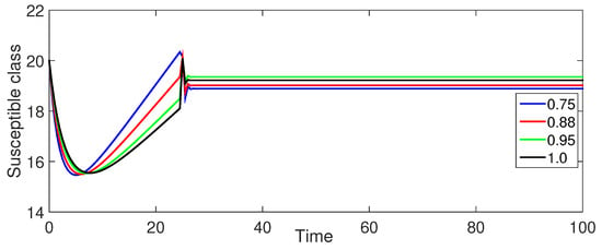
Figure 8.
Numerical illustration for susceptible class at fractional orders ranging from , and with .
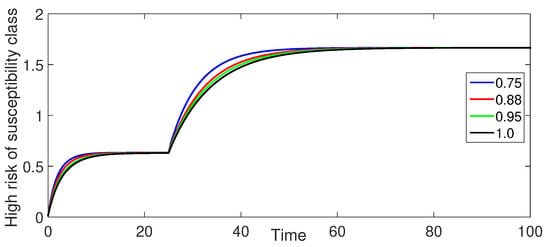
Figure 9.
Numerical illustration for High risk of susceptibility class at fractional orders ranging from and with .
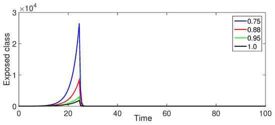
Figure 10.
Numerical illustration for exposed class at fractional orders ranging from , and with .
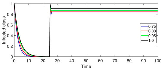
Figure 11.
Numerical illustration for infected class at fractional orders ranging from , and with .
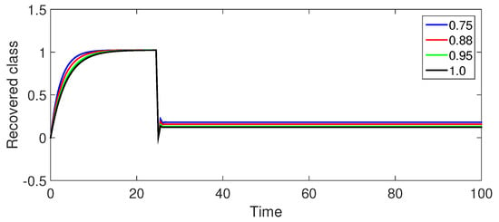
Figure 12.
Numerical illustration for recovered class at fractional orders ranging from , and with .
Overall, the simulations demonstrate the following:
- Fractional Order : Smaller fractional orders lead to a faster disease spread and a quicker initial increase in the exposed population. The transition from -Caputo to -ABC derivative, or the crossover effect, is more pronounced with smaller , highlighting the influence of memory effects on the early stages of the outbreak.
- Increasing Function : The choice of the increasing function affects the model’s dynamics. In general, the crossover effect is less prominent for compared to , suggesting a smoother transition in the model’s behavior.
- Crossover Effect: The crossover effect is evident in all compartments, representing a gradual transition from local behavior (-Caputo derivative) to non-local behavior (-ABC derivative). This transition is more gradual for .
These observations highlight the importance of incorporating memory effects and the crossover effect in modeling disease outbreaks. The -piecewise hybrid fractional derivative approach offers a more realistic and nuanced representation of disease dynamics compared to traditional integer-order models, providing valuable insights for understanding and controlling infectious diseases like Ebola.
Therefore, Figure 3, Figure 4, Figure 5, Figure 6, Figure 7, Figure 8, Figure 9, Figure 10, Figure 11 and Figure 12 provide valuable visual insights into the dynamics of the -piecewise hybrid fractional Ebola model, highlighting the influence of fractional order and crossover effects. They emphasize the importance of incorporating memory effects and demonstrate the potential of this approach for improving the accuracy of EVD modeling and predictions.
9. Conclusions
This study has developed a novel fractional mathematical model to investigate the dynamics of Ebola virus disease (EVD) transmission, incorporating multiple compartments representing different levels of susceptibility and disease states. Our approach utilizes the -Caputo derivative and the -ABC derivative, allowing us to analyze the complex interactions within the population and the effects of memory on disease dynamics. The findings from our analysis reveal several key insights:
The total population size is positive and bounded by , indicating that the model captures the constraints of real-world populations. This aspect is essential for understanding the potential spread of EVD within defined limits.
We identified the disease-free equilibrium point , which serves as a critical threshold for assessing the potential for disease eradication. The parameters defining this equilibrium are crucial for guiding public health interventions.
The basic reproduction number provides a quantitative measure of the epidemic potential of EVD.
The stability analysis indicates that when , small outbreaks will eventually die out, while suggests the possibility of sustained epidemics. This finding emphasizes the importance of targeting control strategies to reduce below unity.
From the sensitivity analysis, we conclude that the infection rate , which governs the speed of disease spread, and the birth rate as well as , which affects the size of the susceptible population, have a significant impact on the EVD model’s dynamics.
The observed crossover effect suggests a critical transition in the disease dynamics near , which could have implications for timing and strategies in outbreak response.
Overall, the results obtained in this work are more important compared to results [32]. This implies that the -piecewise hybrid fractional derivative plays a vital role in simulating the transmission dynamics of the diseases, providing insights into the disease’s spread and potential intervention strategies.
Future Research Directions
- Spatial Dynamics: Incorporate spatial heterogeneity in transmission patterns.
- Detailed Interventions: Model specific interventions like vaccination and contact tracing.
- Environmental Factors: Integrate factors like temperature and sanitation.
- Animal Reservoirs: Explore the role of zoonotic transmission.
- Data Calibration: Refine parameters with detailed datasets.
- Real-World Validation: Validate model predictions against observed outbreaks.
- Other Diseases: Extend the approach to other infectious diseases with complex dynamics.
These directions aim to enhance the realism and applicability of our model, leading to a deeper understanding of EVD and improved strategies for its control.
Author Contributions
Conceptualization, M.A.A.; methodology, M.A.A.; software, M.A.A.; validation, N.M. and K.A.A.; writing—original draft preparation, M.A.A., H.S. and K.A.A.; writing—review and editing, T.A., N.M., A.A., K.A.A. and H.S.; visualization, K.A.A.; supervision and project administration, M.A.A. and K.A.A.; funding acquisition, N.M. All authors have read and agreed to the published version of the manuscript.
Funding
This work was funded by Qassim University.
Data Availability Statement
Data are contained within the article.
Acknowledgments
The Researchers would like to thank the Deanship of Graduate Studies and Scientific Research at Qassim University for financial support (QU-APC-2024-9/1). The authors extend their appreciation to the Islamic University of Madinah.
Conflicts of Interest
The authors declare no conflicts of interest.
References
- World Health Organization (WHO). World Health Statistics 2014. Available online: https://iris.who.int/bitstream/handle/10665/112738/9789240692671_eng.pdf (accessed on 5 October 2024).
- World Health Organization. Ebola Virus Disease (Report); World Health Organization: Geneva, Switzerland, 2019.
- Centers for Disease Control and Prevention (CDC). CDC Urges All US Residents to Avoid Nonessential Travel to Liberia, Guinea and Sierra Leone Because of an Unprecedented Outbreak of Ebola; Centers for Disease Control and Prevention (CDC): Atlanta, GA, USA, 2014.
- Centers for Disease Control and Prevention (CDC). Ebola Outbreak in West Africa 2014; Centers for Disease Control and Prevention (CDC): Atlanta, GA, USA, 2014.
- World Health Organization (WHO). Statement on Ebola in the Democratic Republic of the Congo; World Health Organization (WHO): Geneva, Switzerland, 2017.
- Hodal, K. Ebola Outbreak Declared in Democratic Republic of the Congo after Three Die; The Guardian: London, UK, 2017; ISSN 1756-3224. [Google Scholar]
- Scutti, S.; Goldschmidt, D. Ebola Outbreak Declared in Democratic Republic of Congo; CNN: Atlanta, GA, USA, 2018. [Google Scholar]
- World Health Organization (WHO). Ebola Outbreak in DRC Ends: WHO Calls for International Efforts to Stop Other Deadly Outbreaks in the Country; World Health Organization (WHO): Geneva, Switzerland, 2018.
- Grady, D. Congo’s Ebola Outbreak Is Declared a Global Health Emergency. The New York Times, 17 July 2019. [Google Scholar]
- Gatherer, D. The 2014 Ebola virus disease outbreak in West Africa. J. Gen. Virol. 2014, 95 Pt 8, 1619–1624. [Google Scholar] [CrossRef] [PubMed]
- Longo, D.L.; Kasper, D.L.; Jameson, J.L.; Fauci, A.S.; Hauser, S.L.; Loscalzo, J. (Eds.) Harrison’s Principles of Internal Medicine, 18th ed.; McGraw-Hill: New York, NY, USA, 2011; Chapter 197; ISBN 978-0071748896. [Google Scholar]
- Beeching, N.J.; Fenech, M.; Houlihan, C.F. Ebola Virus Disease. BMJ 2014, 10, G7438. [Google Scholar] [CrossRef] [PubMed]
- Modrow, S.; Falke, D.; Truyen, U.; Schätzl, H. (Eds.) Viruses: Definition, Structure, Classification. In Molecular Virology; Springer: Berlin/Heidelberg, Germany, 2013; pp. 17–30. ISBN 978-3-642-20718-1. [Google Scholar] [CrossRef]
- Ahmad, W.; Rafiq, M.; Abbas, M. Mathematical analysis to control the spread of Ebola virus epidemic through voluntary vaccination. Eur. Phys. J. Plus 2020, 135, 775. [Google Scholar] [CrossRef]
- Nazir, A.; Ahmed, N.; Khan, U.; Mohyud-Din, S.T.; Nisar, K.S.; Khan, I. An advanced version of a conformable mathematical model of Ebola virus disease in Africa. Alex. Eng. J. 2020, 59, 3261–3268. [Google Scholar] [CrossRef]
- Ahmad, W.; Abbas, M. Effect of quarantine on transmission dynamics of Ebola virus epidemic: A mathematical analysis. Eur. Phys. J. Plus 2021, 136, 355. [Google Scholar] [CrossRef]
- Yadav, P.; Jahan, S.; Nisar, K.S. Fractional order mathematical model of Ebola virus under Atangana–Baleanu–Caputo operator. Results Control Optim. 2023, 13, 100332. [Google Scholar] [CrossRef]
- Baller, A.; Padoveze, M.C.; Mirindi, P.; Hazim, C.E.; Lotemo, J.; Pfaffmann, J.; Ndiaye, A.; Carter, S.; Chabrat, M.A.D.; Mangala, S.; et al. Ebola virus disease nosocomial infections in the Democratic Republic of the Congo: A descriptive study of cases during the 2018–2020 outbreak. Int. J. Infect. 2022, 115, 126–133. [Google Scholar] [CrossRef]
- Liu, Q.; Din, A.; Allali, A. Analysis of a multiply delayed stochastic Ebola model based on probability density function with case study. Eur. Phys. J. Plus 2023, 138, 1–18. [Google Scholar] [CrossRef]
- Adu, I.K.; Wireko, F.A.; Nana-Kyere, S.; Appiagyei, E.; Osman, M.A.; Asamoah, J.K.K. Modelling the dynamics of Ebola disease transmission with optimal control analysis. Model. Earth Syst. Environ. 2024, 10, 4731–4757. [Google Scholar] [CrossRef]
- Clancy, C.S.; Smart, G.; Rhoderick, J.F.; O’Donnell, K.L.; Rosenke, R.; Schäfer, A.; Marzi, A. Establishing a mouse model for sexual transmission and male reproductive tract persistence of Ebola virus. J. Infect. Dis. 2023, 228 (Suppl. S7), S554–S558. [Google Scholar] [CrossRef]
- Atangana, A.; Araz, S.İ. New concept in calculus: Piecewise differential and integral operators. Chaos Solitons Fractals 2021, 145, 110638. [Google Scholar] [CrossRef]
- Redhwan, S.S.; Han, M.; Almalahi, M.A.; Alyami, M.A.; Alsulami, M.; Alghamdi, N. Piecewise implicit coupled system under ABC fractional differential equations with variable order. AIMS Math. 2024, 9, 15303–15324. [Google Scholar] [CrossRef]
- Almalahi, M.A.; Aldwoah, K.A.; Shah, K.; Abdeljawad, T. Stability and Numerical Analysis of a Coupled System of Piecewise Atangana–Baleanu Fractional Differential Equations with Delays. Qual. Theory Dyn. Syst. 2024, 23, 105. [Google Scholar] [CrossRef]
- Kattan, D.A.; Hammad, H.A. Existence and Stability Results for Piecewise Caputo-Fabrizio Fractional Differential Equations with Mixed Delays. Fractal Fract. 2023, 7, 644. [Google Scholar] [CrossRef]
- Alazman, I.; Alkahtani, B.S.T. Investigation of novel piecewise fractional mathematical model for COVID-19. Fractal Fract. 2022, 6, 661. [Google Scholar] [CrossRef]
- Shah, K.; Khan, A.; Abdalla, B.; Abdeljawad, T.; Khan, K.A. A mathematical model for Nipah virus disease by using piecewise fractional order Caputo derivative. Fractals 2024, 32, 2440013. [Google Scholar] [CrossRef]
- Alkahtani, B.S.T. Dynamical Analysis of Rubella Disease Model in the Context of Fractional Piecewise Derivative: Simulations with Real Statistical Data. Fractal Fract. 2023, 7, 746. [Google Scholar] [CrossRef]
- Aldwoah, K.A.; Almalahi, M.A.; Shah, K. Theoretical and numerical simulations on the hepatitis B virus model through a piecewise fractional order. Fractal Fract. 2023, 7, 844. [Google Scholar] [CrossRef]
- Nisar, K.S.; Farman, M.; Jamil, K.; Akgul, A.; Jamil, S. Computational and stability analysis of Ebola virus epidemic model with piecewise hybrid fractional operator. PLoS ONE 2024, 19, e0298620. [Google Scholar] [CrossRef]
- Rosa, S.; Ndaïrou, F. Optimal Control Applied to Piecewise-Fractional Ebola Model. Mathematics 2024, 12, 985. [Google Scholar] [CrossRef]
- Abdul-Wahhab, R.D.; Eisa, M.M.; Khalaf, S.L. The study of stability analysis of the Ebola virus via fractional model. Partial. Equs. Appl. Math. 2024, 11, 100792. [Google Scholar] [CrossRef]
- Aldwoah, K.A.; Almalahi, M.A.; Abdulwasaa, M.A.; Shah, K.; Kawale, S.V.; Awadalla, M.; Alahmadi, J. Mathematical analysis and numerical simulations of the piecewise dynamics model of Malaria transmission: A case study in Yemen. AIMS Math. 2024, 9, 4376–4408. [Google Scholar] [CrossRef]
- Almeida, R.; Malinowska, A.B.; Monteiro, M.T.T. Fractional differential equations with a Caputo derivative with respect to a kernel function and their applications. Math. Methods Appl. Sci. 2018, 41, 336–352. [Google Scholar] [CrossRef]
- Almeida, R. A Caputo fractional derivative of a function with respect to another function. Commun. Nonlinear Sci. Numer. Simulat. 2017, 44, 460–481. [Google Scholar] [CrossRef]
- Fernandez, A.; Baleanu, D. Differintegration with respect to functions in fractional models involving Mittag-Leffler functions. In Proceedings of the International Conference on Fractional Differentiation and Its Applications (ICFDA), Amman, Jordan, 16–18 July 2018. [Google Scholar] [CrossRef]
- Atangana, A.; Baleanu, D. New fractional derivative with non-local and non-singular kernel. Therm. Sci. 2016, 20, 757–763. [Google Scholar] [CrossRef]
- Kilbas, A.A.; Srivastava, H.M.; Trujillo, J.J. Theory and applications of fractional differential equations. In North-Holland Mathematicsstudies; Elsevier Science B.V.: Amsterdam, The Netherlands, 2006; Volume 204. [Google Scholar]
- Neves, H.C.C.; Medeiros, M.; Munari, D.B.; Ribeiro, L.C.M.; Tipple, A.F.V. Safety of nursing staff and determinants of adherence to personal protective equipment. Rev. Lat.-Am. Enfermagem 2011, 19, 354–361. [Google Scholar] [CrossRef] [PubMed]
- Makinde, O.D.; Okosun, K.O. Impact of chemo-therapy on optimal control of malaria disease with infected immigrants. BioSystems 2011, 104, 32–41. [Google Scholar] [CrossRef]
- Jarad, F.; Abdeljawad, T. Generalized fractional derivatives and Laplace transform. Discrete Contin. Dyn. Syst. Ser. S 2020, 13, 709–722. [Google Scholar] [CrossRef]
- Fahad, H.M.; Rehman, M.U.; Fernandez, A. On Laplace transforms with respect to functions and their applications to fractional differential equations. Math. Methods Appl. Sci. 2023, 46, 8304–8323. [Google Scholar] [CrossRef]
- Thabet, S.T.; Abdeljawad, T.; Kedim, I.; Ayari, M.I. A new weighted fractional operator with respect to another function via a new modified generalized Mittag–Leffler law. Bound. Value Probl. 2023, 2023, 100. [Google Scholar] [CrossRef]
- Kilbas, A.A.; Saigo, M.; Saxena, R.K. Generalized Mittag-Leffler function and generalized fractional calculus operators. Integral Transform. Spec. Funct. 2004, 15, 31–49. [Google Scholar] [CrossRef]
- Haubold, H.J.; Mathai, A.M.; Saxena, R.K. Mittag-Leffler functions and their applications. J. Appl. Math. 2011, 2011, 298628. [Google Scholar] [CrossRef]
- Agusto, F.B.; Teboh-Ewungkem, M.I.; Gumel, A.B. Mathematical assessment of the effect of traditional beliefs and customs on the transmission dynamics of the 2014 Ebola outbreaks. BMC Med. 2015, 13, 96. [Google Scholar] [CrossRef] [PubMed]
- Nuño, M.; Reichert, T.A.; Chowell, G.; Gumel, A.B. Protecting residential care facilities from pandemic influenza. Proc. Natl. Acad. Sci. USA 2008, 105, 10625–10630. [Google Scholar] [CrossRef]
Disclaimer/Publisher’s Note: The statements, opinions and data contained in all publications are solely those of the individual author(s) and contributor(s) and not of MDPI and/or the editor(s). MDPI and/or the editor(s) disclaim responsibility for any injury to people or property resulting from any ideas, methods, instructions or products referred to in the content. |
© 2024 by the authors. Licensee MDPI, Basel, Switzerland. This article is an open access article distributed under the terms and conditions of the Creative Commons Attribution (CC BY) license (https://creativecommons.org/licenses/by/4.0/).