Multivariable Fractional-Order Controller Design for a Nonlinear Dual-Tank Device

Abstract

Fractional calculus is defined by expanded integer order integration and differentiation. In this paper, multiple mathematical models of a nonlinear dual-tank device are precisely formulated by fractional calculus. Using the accurate model, a multivariable fractional-order controller is designed for nonlinear devices. The merits of the fractional-order design include: (1) control of multivariable nonlinearities, (2) compensation of uncertainties, and (3) elimination of coupling effects. Simulations and experiments are conducted to verify the precision of the fractional order models and the effectiveness of the multivariable fractional-order control system design.

1. Introduction

Tank devices, which are the subject of control in this paper, are widely used in oil, gas, chemical, pharmaceutical, food, and other plants. The chemical products and energy produced in these plants are essential to our daily lives and must operate day and night without interruption. Plants produce products by controlling temperature, pressure, and flow rate to cause the desired chemical and physical reactions in raw materials, and the process is continuous. Chemical products such as iron and resins require precise temperature control because they solidify at lower temperatures. The plant must continue to operate as long as possible after the start of production, and the goals of control are to ensure safety, increase productivity, and improve economic efficiency. In order to achieve these goals, process control research is actively conducted. The dual-tank device used in this paper is widely used in the process field because it heats the material to be heated indirectly, allowing slow and uniform heating of the material, and is stable and resistant to temperature fluctuations.

Many of the phenomena that occur in process systems are mathematically nonlinear, making it difficult to design precise control systems. In general, when designing control systems for nonlinear systems, nonlinear systems are often linearized and linear control theory is applied [1,2,3,4,5]. In this case, however, linearization often degrades the performance of the entire control system and determines the controllable range. For this reason, research has been conducted on adaptive control and optimal control to satisfy the specified control performance, as well as on control systems that handle nonlinear systems [6,7,8,9]. Sliding mode control is one of the control methods for control systems with nonlinear elements. It is applied to servo systems because of its excellent robustness [10,11,12,13,14]. Furthermore, operator theory has been studied as a control theory for handling nonlinear systems. Operator theory can represent a plant as a map from the input space to the output space, allowing control of the system in the time domain. It also has the advantages of easy robust stability analysis in the presence of uncertainty and extensibility to multi-input/output systems, and has been applied to a variety of control objects [15,16,17,18,19,20,21,22].

Process control is a multivariable control in which multiple values such as temperature, flow rate, pressure, and liquid level are controlled simultaneously. In the tank device that is the target of control in this paper the temperature and liquid volume in the tank must be controlled at the same time. When many control variables are controlled simultaneously, each control system generates interference in each other’s input/output. If the model of the control system includes the effects of interference, errors may occur between the actual plant and the model, leading to a reduction in control performance. In control systems where interference exists, unlike single-input single-output control, it is necessary to design the control system and apply stability conditions that take into account the interference that occurs in the plant. Control system design based on operator theory has attracted attention because it considers the bounded-input bounded-output stability of the plant and can be easily extended to multi-input multi-output systems.

In a previous study, the heat exchange and liquid level processes of a dual-tank device were modeled using integer calculus and operator theory to control the liquid temperature and liquid level, respectively, [23]. In that study, a multi-input multi-output control system was designed to perform single-input single-output target-value tracking for the heat exchange process in a dual-tank device and then perform target-value tracking for the liquid level process after the target-value tracking is stabilized. However, the model constructed in that study assumes a constant liquid volume in TANK1, and thus cannot control the liquid level and temperature simultaneously—the temperature rises even when a liquid cooler than the liquid in TANK1 flows into the system. Therefore, it is necessary to develop a new mathematical model for the case of variable liquid volume. In addition, in that study, the control system design is an integer-order control system. The integer-order derivative is a series of derivatives with properties similar to those of ordinary derivatives because the order of the derivatives is an integer, making it a general modeling; however, modeling with fractional-order calculus can represent more complex phenomena than conventional integer-order calculus modeling.

Based on the above, this paper has two objectives. The first is to realize a control system that can simultaneously control liquid temperature and liquid level. In previous studies, heating by a heater was the only way to control the liquid temperature, and the temperature did not decrease even if low-temperature liquid was allowed to flow into the physical model. This paper focuses on the fact that the temperature decreases when low-temperature liquid flows into TANK1 in a real plant, and confirms that the physical model can reproduce the decrease in liquid temperature. Temperature control is performed by using the temperature drop due to pumping liquid as well as heater-based heating as input. Second, modeling is performed in which the liquid temperature and liquid level are expressed in fractional-order derivatives. In other words, in this paper, the goal is to improve modeling accuracy by using fractional calculus for the heat exchange and liquid level processes in the tank device under control. Fractional calculus is a concept that extends the derivative, which is usually expressed in terms of integers, to whole real numbers, and has been applied in various fields of research in recent years [24,25]. It is believed that the use of fractional differential orders allows for simpler expressions of complex phenomena than those of integer orders. The use of fractional order derivatives in modeling controls multivariate nonlinearities, compensates for uncertainties, and eliminates coupling effects. Based on the above objectives, the accuracy of the heat exchange process and liquid level process models expressed in fractional calculus derivatives and the effectiveness of a multivariable fractional-order control system design are verified through simulations and experiments to validate a control system that can simultaneously control liquid temperature and liquid level. Simulation and experiments show that the proposed modeling and control system design using fractional calculus can simultaneously control liquid temperature and liquid level, compensate for uncertainties, and eliminate coupling effects by improving the accuracy of the model.

2. Mathematical Preparation

2.1. Fractional Calculus

Fractional calculus is a calculus that extends the definition of calculus, originally defined only for integers, to include real numbers [26]. Fractional calculus is not a new concept, with early systematic work having been carried out as early as the 19th century. In recent years, fractional calculus has been applied to the field of control in an increasing number of engineering applications. There are many phenomena that can be expressed using fractional calculus, such as the stress generated in a viscoelastic damper, which consists of a spring and damper, and the heat flux generated in a semi-infinitely extending thermocouple. There are several definitions of fractional calculus, but in this paper, the Grünwald–Letnikov definition, which is based on finite differences, is used. This definition can be derived by generalizing the finite difference, which is the defining equation for the derivative. The Grünwald–Letnikov definition is shown in Equation (1).

$$\frac{d^{q}f\left(t\right)}{d{t}^q}\equiv \underset{N\to \infty }{lim}\left({\left(\frac{t-t_0}{N}\right)}^{-q}\sum _{k=0}^{N-1}\frac{\mathsf{\Gamma }(k-q)}{\mathsf{\Gamma }(k+1)\mathsf{\Gamma }(-q)}f\left(t-k\frac{t-t_0}{N}\right)\right)$$

(1)

Since numerical computations by computer cannot realize the computation of the limit contained in Equation (1), the G1-Algorithm expression, as shown in Equation (2), is used in the simulations and experiments.

$$\frac{d^{q}f\left(t\right)}{d{t}^q}=\Delta t^{-q}\sum _{k=0}^{m-1}\frac{\mathsf{\Gamma }(k-q)}{\mathsf{\Gamma }(k+1)\mathsf{\Gamma }(-q)}f\left(t-k\Delta t\right)$$

(2)

2.2. Newmark-$\beta$ Method

In this section, we explain the derivation of numerical solutions of differential equations using fractional calculus. In this paper, the control target is expressed as a fractional differential equation, and its solution must be obtained. However, in general, it is difficult to obtain analytical solutions for fractional differential equations. For example, one study [27] established the basic structure of the exponential Euler difference form for Caputo–Fabrizio fractional-order differential equations (CF-FODEs) with multiple lags. It is necessary to derive a numerical solution, and for this, this paper uses the Newmark-$\beta$ method, which is a method for obtaining a solution by integrating differential equations at each small time interval that is also used in general differential equation analysis [28].

The algorithm of the Newmark-$\beta$ method is shown below. First, the output $y\left(t\right)$ and its first-, second-, and q-order derivatives at time t are described by using two parameters $\gamma$ and $\beta$ as follows.

$$\begin{array}{cc}\hfill y\left(t\right)& =\Delta y\left(t\right)+y(t-1)+\Delta t\dot{y}(t-1)+\left(0.5-\frac{\beta }{\gamma }\right)\Delta t^2\ddot{y}(t-1)\hfill \end{array}$$

(3)

$$\begin{array}{cc}\hfill \dot{y}\left(t\right)& =\dot{y}(t-1)+\frac{\gamma }{\beta \Delta t}\Delta y\left(t\right)\hfill \end{array}$$

(4)

$$\begin{array}{cc}\hfill \ddot{y}\left(t\right)& =\frac{1}{\beta \Delta t^2}\left[\Delta y\left(t\right)+\left(\beta -\frac{\beta }{\gamma }\right)\Delta t^2\ddot{y}(t-1)\right]\hfill \end{array}$$

(5)

$$\begin{array}{cc}\hfill \frac{d^{q}y\left(t\right)}{d{t}^q}& =\frac{1}{\mathsf{\Gamma }(1-q)}\left[I_0+\Delta I_t+I_{t-1}\right]\hfill \end{array}$$

(6)

where $\Delta y\left(t\right)$, $I_0$, $\Delta I_t$, $I_{t-1}$ is as follows.

$$\begin{array}{cc}\hfill \Delta y\left(t\right)& =y\left(t\right)-y(t-1)-\Delta t\dot{y}(t-1)-\left(0.5-\frac{\beta }{\gamma }\right)\Delta t^2\ddot{y}(t-1)\hfill \end{array}$$

(7)

$$\begin{array}{cc}\hfill I_0& =\frac{y\left(0\right)}{t^q}\hfill \end{array}$$

(8)

$$\begin{array}{cc}\hfill \Delta I_t& =\frac{\Delta t^{-q}}{(1-q)(2-q)}\left(\frac{\gamma }{\beta }\right)\left[\Delta y\left(t\right)+(2-q)\left(\frac{\beta }{\gamma }\right)\Delta t\dot{y}(t-1)\right]\hfill \end{array}$$

(9)

$$\begin{array}{cc}\hfill I_{t-1}& =\frac{\Delta t}{2}\left[\frac{\dot{y}\left(0\right)}{t^q}+2\sum _{j=1}^{t-2}\frac{\dot{y}\left(j\right)}{{(t-j\Delta t)}^q}+\frac{\dot{y}(t-1)}{\Delta t^q}\right]\hfill \end{array}$$

(10)

In this way, the fractional first-order differential equation can be replaced by the equation for the variable $\Delta y$, which can be solved to obtain the output $y\left(t\right)$ and its first-, second-, and q-order derivatives at time t, respectively. Depending on how $\gamma$ and $\beta$ are taken, the solution may diverge if the sampling time $\Delta t$ is not sufficiently small.

3. Modeling

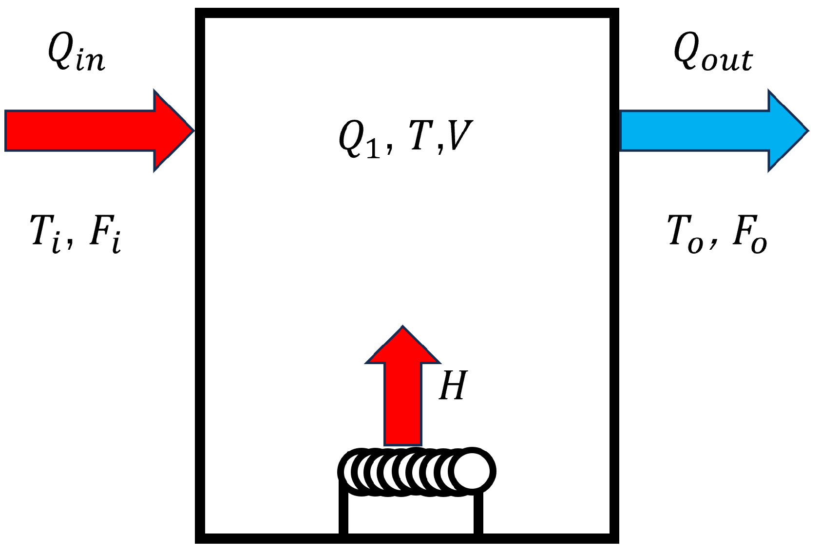
3.1. Fractional Heat Exchange Process

The tank device under control in this paper is a dual tank separated by a solid wall (Figure 1) that uses indirect resistance heating to control the TANK2 liquid temperature. The heat generated from the heater is transferred to TANK2 via the liquid in TANK1, and the temperature of the liquid in TANK2 is controlled by this method. In modeling this device, the parameters shown in

Table 1. Modeling parameters.

Parameter	Definition	Value
${\widehat{D}}_1$	Inside diameter (TANK1)	32 cm
${\widehat{D}}_2$	Inside diameter (TANK2)	11 cm
${\widehat{D}}_0$	Inner diameter	4.0 cm
$\delta$	Thickness of wall	2.0 cm
$h_{\mathrm{b}}$	Distance between botttoms of TANK1 and TANK2	20 cm
$h_{\mathrm{s}}$	Water level (TANK2)	35 cm
${\alpha }_1$	Heat transfer coefficient	$5.0\times {10}^{-5}$ $\mathrm{kJ}/(\mathrm{s}·{\mathrm{cm}}^2·$°C)
${\alpha }_2$	Heat transfer coefficient	$1.5\times {10}^{-4}$ $\mathrm{kJ}/(\mathrm{s}·{\mathrm{cm}}^2·$°C)
k	Thermal conductivity of TANK wall	$1.7\times {10}^{-4}$ $\mathrm{kJ}/(\mathrm{s}·{\mathrm{cm}}^2·$°C)
$C_{\mathrm{TA}}$	TANK1 wall heat capacity	47 $\mathrm{kJ}{/}^{\circ }\mathrm{C}$
$C_2$	Heat capacity of water in TANK2	$5.6$ $\mathrm{kJ}{/}^{\circ }\mathrm{C}$
$C_{\mathrm{TB}}$	TANK2 wall heat capacity	10 $\mathrm{kJ}{/}^{\circ }\mathrm{C}$
$c_{\mathrm{w}}$	Specific heat of water	$4.2\times {10}^{-3}$ $\mathrm{kJ}/{(}^{\circ }\mathrm{C}·\mathrm{g})$
${\rho }_{\mathrm{w}}$	Density of water	$1.0$ $\mathrm{g}/{\mathrm{cm}}^3$
g	acceleration of gravity	$9.8\times {10}^2$ $\mathrm{cm}/{\mathrm{s}}^2$
${\theta }_1\mathrm{i}$	Temperature of influent liquid	18 ${}^{\circ }\mathrm{C}$
${\theta }_1$	Liquid temperature (TANK1)	${}^{\circ }\mathrm{C}$
${\theta }_2$	Liquid temperature (TANK2)	${}^{\circ }\mathrm{C}$
${\widehat{\theta }}_1$	Outer wall temperature	${}^{\circ }\mathrm{C}$
${\widehat{\theta }}_2$	Inner wall temperature	${}^{\circ }\mathrm{C}$
h	Water level (TANK1)	$\mathrm{cm}$
$C_1$	Heat capacity of water in TANK1	$\mathrm{kJ}{/}^{\circ }\mathrm{C}$
$r_{\mathrm{o}}$	Liquid volume of effluent	$\mathrm{L}/\min$
$r_{\mathrm{i}}$	Liquid volume of influent	$\mathrm{L}/\min$
H	Heat supplied by heater	$\mathrm{kJ}/\mathrm{s}$
$\lambda$	Thermal conductivity	$\mathrm{kJ}/(\mathrm{s}·\mathrm{m}·{}^{\circ }\mathrm{C})$

are applied.

The liquid in the tank is kept at a constant temperature by an agitator, and heat is transferred by heat conduction within the solid wall of the tank. Heat conduction is a phenomenon in which heat is transferred by a temperature gradient within the same material, and the amount of heat follows Fourier’s law of heat conduction. If the heat flux moving per unit time is $q_{\mathrm{HF}}$$[\mathrm{J}/\mathrm{s}·{\mathrm{m}}^2]$ and the thermal conductivity of the medium is $\lambda$$[\mathrm{J}/\mathrm{s}·{\mathrm{m}}^2·{}^{\circ }\mathrm{C}]$, heat conduction within the same material can be expressed by Equation (11) to obtain the temperature distribution $\theta \left(x\right)$ of the medium at position x.

$$\begin{array}{c}\hfill q_{\mathrm{HF}}=\lambda \frac{d\theta \left(x\right)}{dx}\end{array}$$

(11)

Here, the thermal conductivity $\lambda$ is a specific value for each medium material. Next, we consider the heat exchange that takes place between the liquid in the tank and the solid wall of the tank. The heat exchange phenomenon that takes place between two different kinds of objects is called heat transfer, and the heat flux $q_{\mathrm{HF}}$$[\mathrm{J}/\mathrm{s}·{\mathrm{m}}^2]$ resulting from this is obtained from the heat transfer coefficient $\alpha$$[\mathrm{J}/\mathrm{s}·{\mathrm{m}}^2·\mathrm{K}]$ and the temperature difference between the objects $\Delta \theta$$\left[\mathrm{K}\right]$ by Equation (12).

$$\begin{array}{c}\hfill q_{\mathrm{HF}}=\alpha \Delta \theta \end{array}$$

(12)

Heat exchange is a series of phenomena in which heat is transferred by heat conduction and heat transfer, and the amount of heat transferred is expressed as the product of a coefficient and a temperature difference in both phenomena.

The amount of heat transferred by heat conduction occurring within the side of the tank solid wall at a radial distance r from the center axis of TANK2, $Q_s$$[\mathrm{J}/\mathrm{s}]$, is expressed by the product of heat flux and heat transfer area using Equation (13).

$$\begin{array}{c}\hfill Q_s=2\pi r(h-(h_b+\delta ))\lambda \frac{d\theta \left(r\right)}{dr}\end{array}$$

(13)

Integrating Equation (13) with respect to temperature $\theta$, the amount of heat transferred within the solid wall is expressed by Equation (14), using the surface temperature of the solid walls ${\widehat{\theta }}_2$ and ${\widehat{\theta }}_1$.

$$\begin{array}{c}\hfill Q_s=\frac{2\pi \lambda (h-(h_b+\delta ))}{ln\left(\frac{{\widehat{D}}_2+2\delta }{{\widehat{D}}_2}\right)}({\widehat{\theta }}_2-{\widehat{\theta }}_1)\end{array}$$

(14)

Assuming that the amount of heat transferred by heat transfer between the liquid in the tank and the solid wall is equal to the amount of heat transferred by heat conduction in the solid wall, the amount of heat $Q_s$ transferred from the liquid in TANK1 to the liquid in TANK2 by heat exchange at the tank side can be expressed by Equation (15).

$$\begin{array}{c}\hfill Q_s=\frac{\pi (h-(h_b+\delta ))}{\frac{1}{{\alpha }_1({\widehat{D}}_2+2\delta )}+\frac{1}{2k}ln\left(\frac{{\widehat{D}}_2+2\delta }{{\widehat{D}}_2}\right)+\frac{1}{{\alpha }_2{\widehat{D}}_2}}({\theta }_1-{\theta }_2)\end{array}$$

(15)

Similarly, the heat quantity $Q_b$$[\mathrm{J}/\mathrm{s}]$ transferred from the liquid in TANK1 to the liquid in TANK2 by heat exchange at the tank bottom is expressed by Equation (16).

$$\begin{array}{c}\hfill Q_b=\frac{\pi {\widehat{D}}_2^2}{4(\frac{\delta }{\lambda }+\frac{1}{{\alpha }_1}+\frac{1}{{\alpha }_2})}({\theta }_1-{\theta }_2)\end{array}$$

(16)

From Equations (15) and (16), the heat quantity $Q_a$$[\mathrm{J}/\mathrm{s}]$ transferred from the liquid in TANK1 to the liquid in TANK2 due to the heat exchange that occurs throughout the tank is expressed by Equation (17).

$$\begin{array}{c}\hfill Q_a=Q_s+Q_b=k({\theta }_1-{\theta }_2)\end{array}$$

(17)

k is expressed in Equation (18).

$$\begin{array}{cc}\hfill k& =\frac{\pi (h-(h_b+\delta ))}{\frac{1}{{\alpha }_1({\widehat{D}}_2+2\delta )}+\frac{1}{2k}ln\left(\frac{{\widehat{D}}_2+2\delta }{{\widehat{D}}_2}\right)+\frac{1}{{\alpha }_2{\widehat{D}}_2}}+\frac{\pi {\widehat{D}}_2^2}{4(\frac{\delta }{\lambda }+\frac{1}{{\alpha }_1}+\frac{1}{{\alpha }_2})}\hfill \end{array}$$

(18)

Next, the concept of the heat balance of the tank is explained. Let $Q_i,Q_o$$\left[\mathrm{J}\right]$ be the heat value, H$\left[\mathrm{J}\right]$ be the heater output, $T_i,T_o$$\left[\mathrm{C}\right]$ be the liquid temperature, $F_i,F_o$$[{\mathrm{m}}^3/\mathrm{s}]$ be the flow rate, V$\left[{\mathrm{m}}^3\right]$ be the liquid volume, $c_p$$[\mathrm{kJ}/\mathrm{kg}·\mathrm{K}]$ be the specific heat, and $\rho$$[\mathrm{kg}/{\mathrm{m}}^3]$ be the density. Then, Equation (19) shows the equation for the heat quantity change in the tank for the heat quantity flowing in, the heat quantity flowing out, and the heat quantity supplied from the heater in Figure 2.

$$\begin{array}{c}\hfill \frac{d{Q}_1}{dt}=Q_{in}-Q_{out}+H\end{array}$$

(19)

The heat quantity Q can be expressed as $Q=\rho c_{p}VT$, and is substituted into the Equation (19).

$$\begin{array}{c}\hfill \rho c_p\frac{d\left\{VT\right\}}{dt}=F_i\rho c_p{T}_i-F_o\rho c_p{T}_o+H\end{array}$$

(20)

Equation (20) can be transformed as in Equation (21), because in this paper we are considering the case where the liquid volume in the tank changes for TANK1.

$$\begin{array}{c}\hfill V\frac{dT}{dt}=F_i{T}_i-F_o{T}_o+\frac{1}{\rho c_p}H-T\frac{dV}{dt}\end{array}$$

(21)

Since the time variation of the heat quantity related to the liquid inside TANK1 and TANK2 can be considered to be equal to the heat balance of each liquid over a small time period, the heat quantity and heat balance equations derived above can be used to formulate the equations for each tank. In TANK1, the amount of heat change in a small time period is determined by the heat supplied from the control input, the heat flow rate that varies with the liquid entering and leaving the tank, the amount of heat transferred by heat exchange, and the amount of heat absorbed by the solid walls of the tank. In TANK2, it is determined by the amount of heat transferred by the heat exchange and the amount of heat absorbed by the solid wall of the tank.

Next, the heat exchange model equation for a dual-tank device is expressed using fractional calculus. In previous studies, it has been found that heat transfer phenomena can be described more accurately by expressing the amount of heat absorbed by the tank solid walls in fractional calculus. The heat transfer model is extended to a fractional dimension in this paper, which can represent the outflow of heat from the solid wall of TANK1 and the change in liquid temperature near the individual tank walls caused by the flow of liquid in the tank. A model expressing the amount of heat absorbed by the solid wall of the tank in fractional calculus is shown in Equations (22) and (23).

$$\{\begin{array}{}\mathrm{(22)}& \begin{array}{cc}\hfill C_1\frac{d{\theta }_1}{dt}& ={\rho }_w{c}_w{r}_i{\theta }_{1i}-{\rho }_w{c}_w{r}_0{\theta }_1+H\hfill \\ \hfill & +k\left({\theta }_2-{\theta }_1\right)-{\chi }_q\frac{d^q{\theta }_1}{d{t}^q}\hfill \\ \hfill & -{\rho }_w{c}_w{\theta }_1\frac{dV}{dt}\hfill \end{array}\mathrm{(23)}& \hfill C_2\frac{d{\theta }_2}{dt}& =k({\theta }_1-{\theta }_2)-{\chi }_p\frac{d^p{\theta }_2}{d{t}^p}\hfill \end{array}$$

${\chi }_q$ and ${\chi }_p$ are expressed as in Equations (24) and (25).

$$\begin{array}{c}\hfill {\chi }_q=\frac{d^{1-q}{C}_{TA}}{d{t}^{1-q}}\end{array}$$

(24)

$$\begin{array}{c}\hfill {\chi }_p=\frac{d^{1-p}{C}_{TB}}{d{t}^{1-p}}\end{array}$$

(25)

The advantage of modeling a heat exchange process such as Equations (22) and (23) using fractional-order derivatives over existing modeling is that it can produce a greater variety of waveforms than conventional modeling using integer-order derivatives. Typically, heat exchange modeling is represented using integer-order derivatives; however, the heat exchange modeling used in this paper uses fractional-order derivatives and can model phenomena that cannot be represented by conventional modeling.

From Equations (22) and (23), the differential Equation (26) is derived.

$$\begin{array}{cc}\hfill C_1& C_{2}B\frac{d^2{\theta }_2}{d{t}^2}+(C_1+C_2+{\rho }_w{c}_w{r}_i{C}_{2}B)\frac{d{\theta }_2}{dt}+{\rho }_w{c}_w{r}_i{\theta }_2+({\rho }_w{c}_w{r}_{i}B{\chi }_p+{\chi }_p)\frac{d^p{\theta }_2}{d{t}^p}\hfill \\ \hfill & +{\chi }_q\frac{d^q{\theta }_2}{d{t}^q}+C_1{\chi }_{p}B\frac{d^{p+1}{\theta }_2}{d{t}^{p+1}}+C_2{\chi }_{q}B\frac{d^{q+1}{\theta }_2}{d{t}^{q+1}}+{\chi }_q{\chi }_{p}B\frac{d^{p+q}{\theta }_2}{d{t}^{p+q}}={\rho }_w{c}_w{r}_i{\theta }_{1i}+H\hfill \end{array}$$

(26)

Solving Equation (26) for ${\theta }_2$ yields a model of the heat exchange process. The coefficients ${\chi }_q$ and ${\chi }_p$ are determined by considering the dimension of the model. Specifically, the dimension of ${\chi }_q$ is $[\mathrm{J}/\mathrm{K}·{\mathrm{s}}^{1-\mathrm{q}}]$ and that of ${\chi }_p$ is $[\mathrm{J}/\mathrm{K}·{\mathrm{s}}^{1-\mathrm{p}}]$. This confirms that the dimensions of the left and right sides of the heat balance equation match.

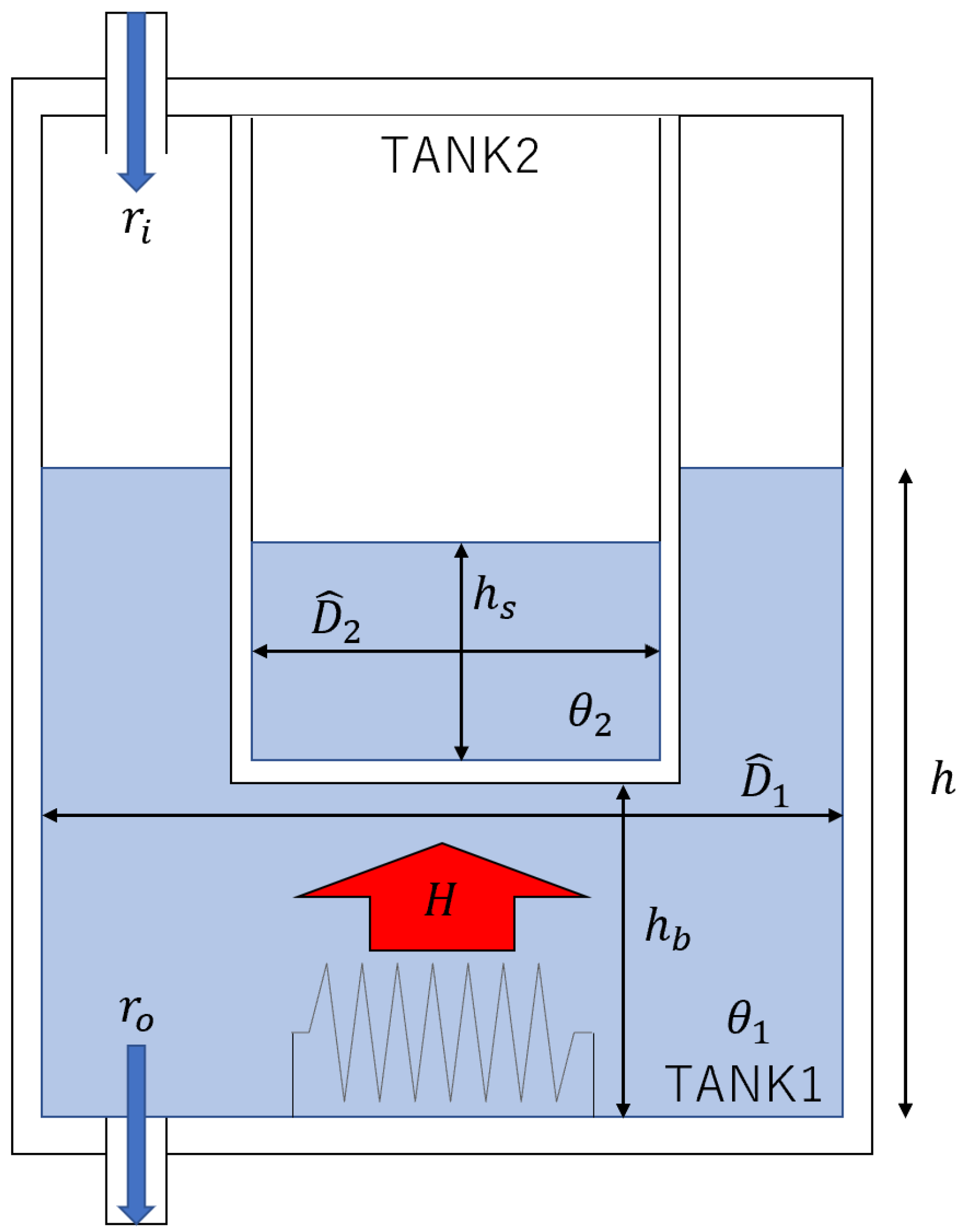
3.2. Fractional Liquid Process

The area A of the liquid surface of TANK1 and the area a of the outlet at the bottom of TANK1 are expressed by Equations (27) and (28).

$$\begin{array}{cc}\hfill A& =\frac{\pi }{4}\left[{\widehat{D}}_1^2-{\left({\widehat{D}}_2+2\delta \right)}^2\right]\hfill \end{array}$$

(27)

$$\begin{array}{cc}\hfill a& =\frac{\pi {\widehat{D}}_0^2}{4}\hfill \end{array}$$

(28)

Letting the inflow into TANK1 be $r_i\left(t\right)$ and the outflow be $r_o\left(t\right)$, Equation (29) is obtained for the time variation of the liquid level $h\left(t\right)$ in TANK1.

$$A\dot{h}\left(t\right)=r_i\left(t\right)-r_o\left(t\right)$$

(29)

The inflow $r_i\left(t\right)$ is the control input and is observable. The outflow $r_o\left(t\right)$ is expressed as the product of the cross-sectional area of the outlet and the velocity of the outflow. The velocity $v\left(t\right)$ at which the liquid in the container flows out through the small hole is obtained from Torricelli’s theorem and is expressed as in Equation (30).

$$v\left(t\right)=\sqrt{2gh\left(t\right)}$$

(30)

Therefore, the outflow from TANK1 is obtained as in Equation (31).

$$r_o\left(t\right)=a\sqrt{2gh\left(t\right)}$$

(31)

From Equations (29)–(31), we obtain Equation (32) as the model equation for the liquid level system.

$$\dot{h}\left(t\right)=\frac{1}{A}{r}_i\left(t\right)-\frac{a}{A}\sqrt{2gh\left(t\right)}$$

(32)

Here, the inflow rate $r_i\left(t\right)$ has a role as a cooling input for liquid temperature control in addition to its role as an input for liquid level control in the dual-tank device used in this paper. Therefore, the inflow rate $r_i\left(t\right)$ includes the interference from the heater in addition to the input $r_i^{\prime }\left(t\right)$ from the pump, and is considered to be expressed by Equation (33).

$$\begin{array}{c}\hfill r_i\left(t\right)=r_i^{\prime }\left(t\right)+\frac{1}{\rho c_w({\theta }_1-{\theta }_i)}H\end{array}$$

(33)

Next, the liquid level model of the tank is expressed using fractional order derivatives. In a real plant, the liquid level oscillates due to the effects of circulators and pumping of liquid. In this paper, this is expressed as uncertainty due to perturbation by fractional calculus, and Equation (34) is added to the liquid level.

$$\begin{array}{cc}\hfill & D^{q_w}\left(G_{1}sin\left({\omega }_{1}t\right)+G_{2}cos\left({\omega }_{2}t\right)\right)\hfill \\ \hfill \simeq & {\left(G_1{\omega }_1\right)}^{q_w}\left[sin\left({\omega }_{1}t+\frac{\pi q_w}{2}\right)+\frac{{\left({\omega }_{1}t\right)}^{-1-q_w}}{\mathsf{\Gamma }(-q_w)}+\frac{{\left({\omega }_{1}t\right)}^{-3-q_w}}{\mathsf{\Gamma }(-q_w-2)}\right]\hfill \\ \hfill +& {\left(G_2{\omega }_2\right)}^{q_w}\left[cos\left({\omega }_{2}t+\frac{\pi q_w}{2}\right)+\frac{{\left({\omega }_{2}t\right)}^{-2-q_w}}{\mathsf{\Gamma }(-q_w-1)}+\frac{{\left({\omega }_{2}t\right)}^{-4-q_w}}{\mathsf{\Gamma }(-q-3)}\right]\hfill \end{array}$$

(34)

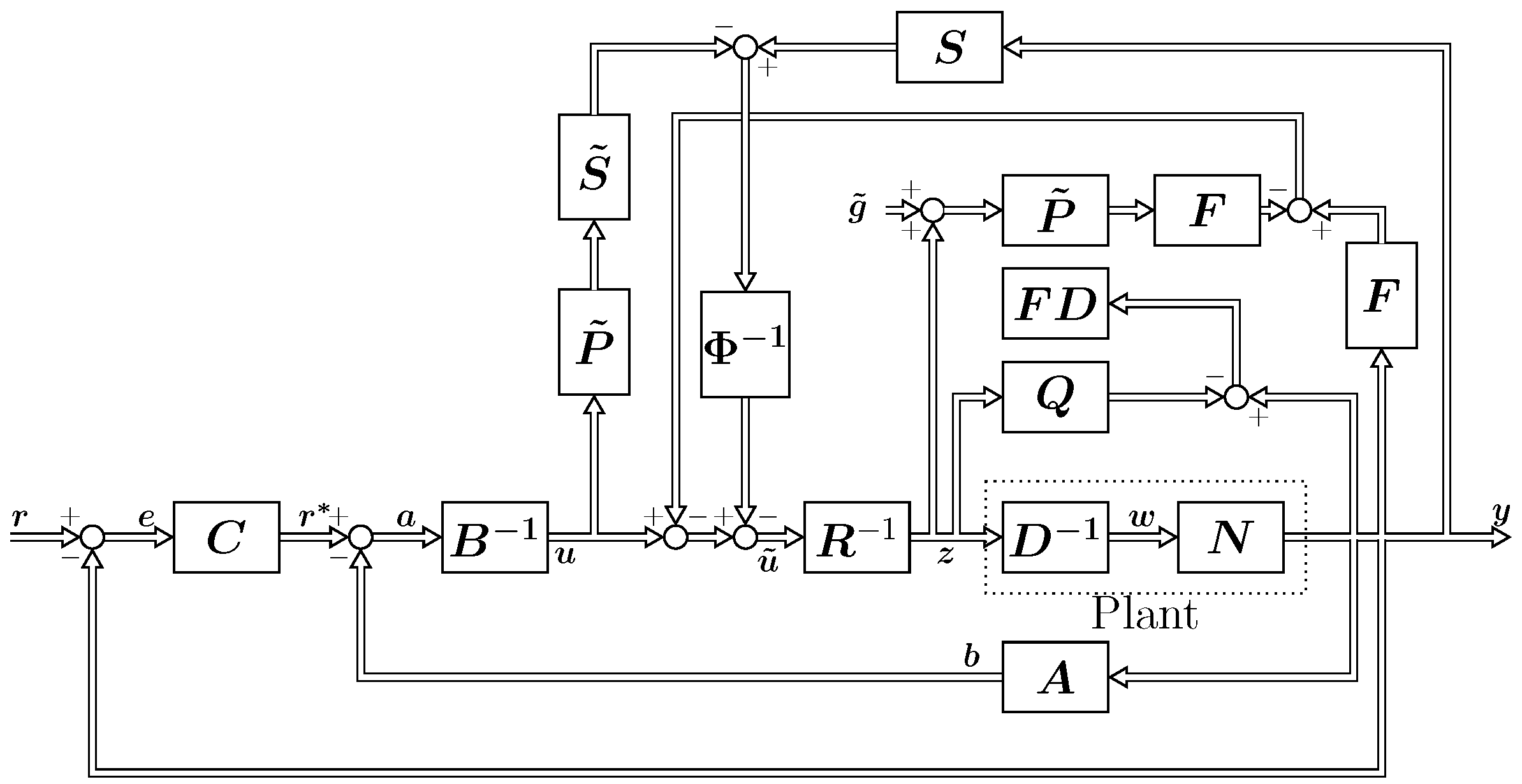
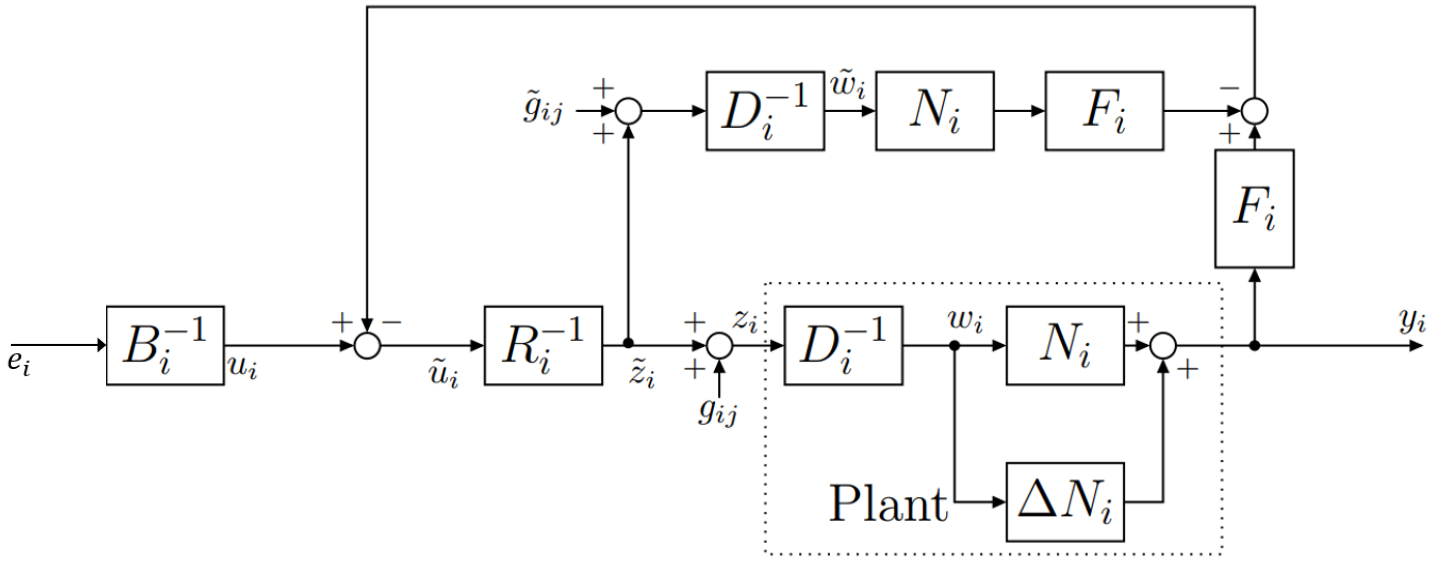
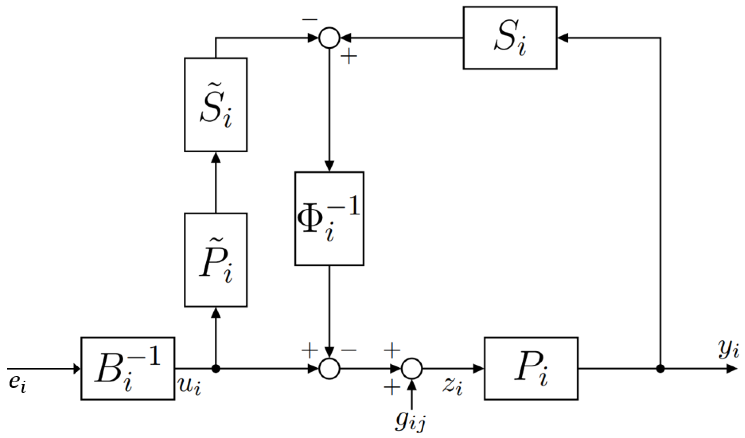
4. Multivariable Fractional-Order Nonlinear Control Feedback System Design

Comparison with existing control methods is performed before designing the control system. The authors of [29] introduced a fractional-order integral derivative controller for a class of integrating systems involving time delays. The stability region is explored through the complex root boundary analysis, which explicitly provides the search space of fractional-order integral derivative controller parameters for integrating time delay systems of any order. The authors of [30] proposed a hybrid fuzzy fractional order proportional integral-fractional order proportional derivative controller as a new expert control technique to tackle automatic generation control profitably in isolated and interconnected multi-area power systems. These control methods are based on a control system design that uses fractional calculus. Therefore, in this paper, modeling using fractional calculus is performed to improve the accuracy of models in chemical plants, and control systems are designed based on operator theory. The advantage of control system design based on operator theory is that it facilitates robust stability analysis in the presence of uncertainty and is highly scalable to multi-input/output systems. A nonlinear feedback control system based on operator theory is designed using the models of the heat exchange process and liquid level process of the tank system constructed in the previous section. An overview of the proposed method is shown in Figure 3. For the operators in Figure 3, $\mathit{N}=(N_1,N_2)$, $\mathit{D}=(D_1,D_2)$ represent the plant and $\mathit{A}=(A_1,A_2)$, $\mathit{B}=(B_1,B_2)$, $\mathit{S}=(S_1,S_2)$, $\mathit{F}=(F_1,F_2)$, $\tilde{\mathit{P}}=({\tilde{P}}_1,{\tilde{P}}_2)$, $\mathsf{\Phi }=({\mathsf{\Phi }}_1,{\mathsf{\Phi }}_2)$, $\mathit{R}=(R_1,R_2)$, $\mathit{C}=(C_1,C_2)$ represent the controller.

4.1. Fractional Liquid Temperature Control Design

Transforming the model equation derived in the previous section, we obtain the plant $P_1:Z_1\to Y_1$. The operators $N_1,D_1^{-1}$ satisfying right factorization $P_1\left(z_1\right)\left(t\right)=N_1{D}_1^{-1}\left(z_1\right)\left(t\right)$ are shown in Equations (35) and (36).

$$\begin{array}{cc}\hfill & N_1:\left\{\begin{array}{c}{C}_1{C}_{2}B\frac{d^2{x}_1\left(t\right)}{d{t}^2}+\left({\rho }_w{c}_w{r}_i+k\right)B{\chi }_p\frac{d^p{x}_1\left(t\right)}{d{t}^p}\hfill \\ +\left(C_1+C_2+C_{2}B{\rho }_w{c}_w{r}_i\right)\frac{d{x}_1\left(t\right)}{dt}+{\rho }_w{c}_w{r}_i{x}_1\left(t\right)\hfill \\ +{\chi }_q\frac{d^q{x}_1\left(t\right)}{d{t}^q}+C_1{\chi }_{p}B\frac{d^{p+1}{x}_1\left(t\right)}{d{t}^{p+1}}+C_2{\chi }_{q}B\frac{d^{q+1}{x}_1\left(t\right)}{d{t}^{q+1}}\hfill \\ +{\chi }_q{\chi }_{p}B\frac{d^{p+q}{x}_1\left(t\right)}{d{t}^{p+q}}=w_1\left(t\right)\hfill \\ {\theta }_2\left(t\right)=x_1\left(t\right)\hfill \end{array}\right.\hfill \end{array}$$

(35)

$$\begin{array}{cc}\hfill & D_1:z_1\left(t\right)=I\left(w_1\left(t\right)\right)\hfill \end{array}$$

(36)

Next, we design controllers $A_1,B_1$ that satisfy the Bezoo equality $A_1{N}_1+B_1{D}_1=M$. Let M be a unimodular operator. When $A_1,B_1$ is a stable operator satisfying the Bezoo equation, the plant has a right-irreducible decomposition and the nonlinear feedback system becomes stable. The operators designed using the design coefficient $K_t$ are shown in Equations (37) and (38).

$$\begin{array}{cc}\hfill A_1:b_1\left(t\right)& =\left(1-K_t\right)\left(C_1{C}_{2}B\frac{d^2{\theta }_2\left(t\right)}{d{t}^2}\right.+\left(C_1+C_2+C_{2}B{\rho }_w{c}_w{r}_i\right)\frac{d{\theta }_2\left(t\right)}{dt}\hfill \\ \hfill +& {\rho }_w{c}_w{r}_i{\theta }_2\left(t\right)+\left({\rho }_w{c}_w{r}_i+k\right)B{\chi }_p\frac{d^p{\theta }_2\left(t\right)}{d{t}^p}+{\chi }_q\frac{d^q{\theta }_2\left(t\right)}{d{t}^q}+C_1{\chi }_{p}B\frac{d^{p+1}{\theta }_2\left(t\right)}{d{t}^{p+1}}\hfill \\ \hfill +& C_2{\chi }_{q}B\frac{d^{q+1}{\theta }_2\left(t\right)}{d{t}^{q+1}}+\left.{\chi }_q{\chi }_{p}B\frac{d^{p+q}{\theta }_2\left(t\right)}{d{t}^{p+q}}\right)\hfill \end{array}$$

(37)

$$\begin{array}{cc}\hfill B_1:e_1\left(t\right)& =K_t{u}_1\left(t\right)\hfill \end{array}$$

(38)

A tracking compensator was designed to compensate for tracking performance. In Figure 3, $C_{1_m}$, $C_{21}$ is a follow-up compensator that operates with the difference between TANK2 temperature ${\theta }_2$ and target temperature as input and a controller that calculates the amount of liquid pumped based on the difference in liquid temperature, and $C_{1_s}$ is a controller that operates with TANK1 temperature ${\theta }_1$ as feedback. $C_{1_s}$ is a follow-up compensator that operates with the TANK1 temperature ${\theta }_1$ as feedback.

$$\begin{array}{cc}\hfill & C_{1_m}:r_{1_m}\left(t\right)=K_{P_{t1}}{\tilde{r}}_1\left(t\right)+K_{I_{t1}}{\int }_{t_0}^t{\tilde{r}}_1\left(\tau \right)d\tau \hfill \end{array}$$

(39)

$$\begin{array}{cc}\hfill & C_{1_s}:r_{1_s}\left(t\right)=K_{P_{t2}}{e}_{1_m}\left(t\right)+K_{I_{t2}}{\int }_{t_0}^t{e}_{1_m}\left(\tau \right)d\tau \hfill \end{array}$$

(40)

$$\begin{array}{cc}\hfill & C_{21}:r_{21}\left(t\right)=K_{P_{tw}}{\tilde{r}}_1\left(t\right)+K_{I_{tw}}{\int }_{t_0}^t{\tilde{r}}_1\left(\tau \right)d\tau \hfill \end{array}$$

(41)

4.2. Fractional Liquid Level Control Design

Similar to the liquid temperature control design, the right-hand decomposition $N_2,D_2$ and stabilizing compensators $A_2,B_2$ of the plant are designed as follows. where $K_w$ is the design coefficient.

$$\begin{array}{cc}\hfill & N_2:\left\{\begin{array}{c}{\dot{x}}_2\left(t\right)=w_2\left(t\right)-\frac{a}{A}\sqrt{2g{x}_2\left(t\right)}\hfill \\ y_2\left(t\right)=x_2\left(t\right)\hfill \end{array}\right.\hfill \end{array}$$

(42)

$$\begin{array}{cc}\hfill & \Delta N_2:D^q\left(G_{1}sin\left({\omega }_{1}t\right)+G_{2}cos\left({\omega }_{2}t\right)\right)\hfill \end{array}$$

(43)

$$\begin{array}{cc}\hfill & D_2:u_2\left(t\right)=A{w}_2\left(t\right)\hfill \end{array}$$

(44)

$$\begin{array}{cc}\hfill & A_2:b_2\left(t\right)=\left(1-K_w\right)\left({\dot{y}}_2\left(t\right)+\frac{a}{A}\sqrt{2g{y}_2\left(t\right)}\right)\hfill \end{array}$$

(45)

$$\begin{array}{cc}\hfill & B_2:e_2\left(t\right)=\frac{K_p}{A}{u}_2\left(t\right)\hfill \end{array}$$

(46)

where for the signal $z_2\left(t\right)$ appearing at the plant $N_2$, $D_2$, the interference from the heater shown during modeling is included, in addition to the liquid level control input $u_2\left(t\right)$. The tracking compensator is designed in the same way.

$$\begin{array}{c}\hfill C_2:r_2\left(t\right)=K_{Pw}{\tilde{r}}_2\left(t\right)+K_{Iw}{\int }_{t_0}^t{\tilde{r}}_2\left(\tau \right)d\tau \end{array}$$

(47)

4.3. Interference Design

In the dual-tank device under control in this paper, when liquid temperature and liquid level are controlled simultaneously, each control input/output affects the other control input/output, resulting in interference. Therefore, the design must take interference into account. The effect of interference on liquid temperature control and liquid level control is expressed using the operator G. In the heat exchange process, the liquid is heated by a heater, but the temperature also changes due to external inflow of liquid. Therefore, when liquid is pumped to control the liquid level in the liquid level control system, interference occurs with the temperature control system. This can be expressed in a mathematical expression using the operator $G_{12}:U_2\to U_1$, which gives Equation (48).

$$\begin{array}{c}\hfill G_{12}\left(u_2\left(t\right)\right)={\rho }_w{c}_w{\theta }_{1i}{u}_2\left(t\right)\end{array}$$

(48)

Next, the liquid level process is designed in the same way. In the liquid temperature control method used in this paper, the controller $C_{21}$ orders the liquid to be pumped to TANK1 if the liquid temperature becomes too high. This changes the amount of liquid pumped and affects the liquid level control operation. However, the output from the heater does not become zero during this time. This results in the need for extra cooling for the amount of heat from the heater, so the amount of liquid pumped increases according to the amount of heat supplied by the heater. This can be expressed in a mathematical expression using the operator $G_{21}:U_1\to U_2$, which gives Equation (49).

$$\begin{array}{cc}\hfill & G_{21}\left(u_1\left(t\right)\right)=\frac{u_1\left(t\right)}{{\rho }_w{c}_w({\theta }_1-{\theta }_{1i})}\hfill \end{array}$$

(49)

4.4. Uncertainty Compensation Design

The feedback system of uncertainty compensation is shown in Figure 4.

In the actual process, the dual-tank device has uncertainties that are not included in the model. The process $P_i+\Delta P_i$ including this uncertainty is expressed as in Equation (50).

$$\begin{array}{c}\hfill P_i+\Delta P_i=(N_i+\Delta N_i)D_i^{-1}\end{array}$$

(50)

As an example, consider the case where $i=1$, $j=2$. In this case, the signal ${\tilde{u}}_1$ can be expressed as in Equation (51), in which ${\tilde{g}}_{12}$ is the ideal interference without uncertainty.

$$\begin{array}{cc}\hfill {\tilde{u}}_1& =u_1-F_1\left(y_1\right)+F_1{N}_1\left({\tilde{\omega }}_1\right)\hfill \\ \hfill & =R_1(D_1\left({\tilde{\omega }}_1\right)-{\tilde{g}}_{12})\hfill \end{array}$$

(51)

If $R_1$ is designed as a linear operator, Equation (51) is expressed as in Equation (52).

$$\begin{array}{c}\hfill R_1{D}_1\left({\tilde{\omega }}_1\right)-F_1{N}_1\left({\tilde{\omega }}_1\right)=u_1-F_1\left(y_1\right)+R_1\left({\tilde{g}}_{12}\right)\end{array}$$

(52)

The signal ${\tilde{\omega }}_1$ can be transformed as in Equation (53) since $D_1^{-1}$ is a linear operator.

$$\begin{array}{c}\hfill {\tilde{\omega }}_1=D_1^{-1}({\tilde{z}}_1+{\tilde{g}}_{12})=D_1^{-1}\left({\tilde{z}}_1\right)+D_1^{-1}\left({\tilde{g}}_{12}\right)\end{array}$$

(53)

Substituting the signal ${\tilde{\omega }}_1$ into Equation (51) and transforming it, we obtain Equation (54).

$$\begin{array}{c}\hfill R_1\left({\tilde{z}}_1\right)+R_1\left({\tilde{g}}_{12}\right)-F_1{P}_1\left({\tilde{z}}_1\right)-F_1{P}_1\left({\tilde{g}}_{12}\right)\\ \hfill =u_1-F_1\left(y_1\right)+R_1\left({\tilde{g}}_{12}\right)\end{array}$$

(54)

Here, by designing $F_1{P}_1=I$ and $R_1=I$, where I is an identity map, it is expressed as in Equation (55).

$$\begin{array}{c}\hfill u_1+{\tilde{g}}_{12}=F_1\left(y_1\right)\end{array}$$

(55)

Thus, the ideal output and the output with uncertainty are equal, and the uncertainty can be compensated.

4.5. Coupling Effect Elimination Design

The control system that eliminates coupling effects is shown in Figure 5.

In this section, we consider the case $i=1,j=2$. When controlling liquid temperature and liquid level simultaneously, there is mutual interference in terms of the heat supplied and the amount of liquid pumped. In Figure 3, $z_1\left(t\right)$ is represented by Equation (56).

$$\begin{array}{cc}\hfill z_1\left(t\right)=& u_1+g_{12}-{\varphi }_1^{-1}{S}_{1}P\left(z_1\right)+{\varphi }_1^{-1}{\tilde{S}}_1{\tilde{P}}_1\left(u_1\right)\hfill \end{array}$$

(56)

where ${\varphi }_1$ and ${\varphi }_1^{-1}$ can be transformed as in Equation (57) when designed as linear operators.

$$\begin{array}{c}\hfill {\varphi }_1^{-1}({\varphi }_1+S_1{P}_1)\left(z_1\right)=g_{12}+{\varphi }_1^{-1}({\varphi }_1+{\tilde{S}}_1{\tilde{P}}_1)\left(u_1\right)\end{array}$$

(57)

Therefore, the controller is designed to satisfy the relationship in Equation (57). Each operator is designed with $S_1=I$ and ${\varphi }^{-1}\left({\alpha }_1\right)\left(t\right)=\frac{1}{n}{\alpha }_1$, where $\frac{1}{n}{\alpha }_1$ is the bounded signal and n is the design parameter. By considering ${\varphi }_1^{-1}$ and ${\varphi }_1$, we obtain Equation (58).

$$\begin{array}{c}\hfill z_1\to u_1\end{array}$$

(58)

Equation (58) shows that the input signal $Z_1$ and the output $U_1$ of operator $B_1^{-1}$ are equal, thus eliminating coupling effects.

4.6. Control System Design Details

Finally, the details of the control system design used in this paper are shown in Figure 6. For plants $D,N,\Delta N$ and controllers $A,B,R,C,F,S,\tilde{S},\tilde{P},\mathsf{\Phi }$ in the control system, subscripts of 1 are related to the liquid temperature control system and those of 2 to the liquid level control system. $C_{21}$ refers to a controller that calculates the amount of liquid pumped based on the difference in liquid temperature, and $G_{12},G_{21}$ refers to interference between the liquid temperature control system and the liquid level control system. Figure 6 shows a detail of the control system design proposed in this paper, and Figure 3 shows a compact version of the control system design in Figure 6.

5. Results and Discussion

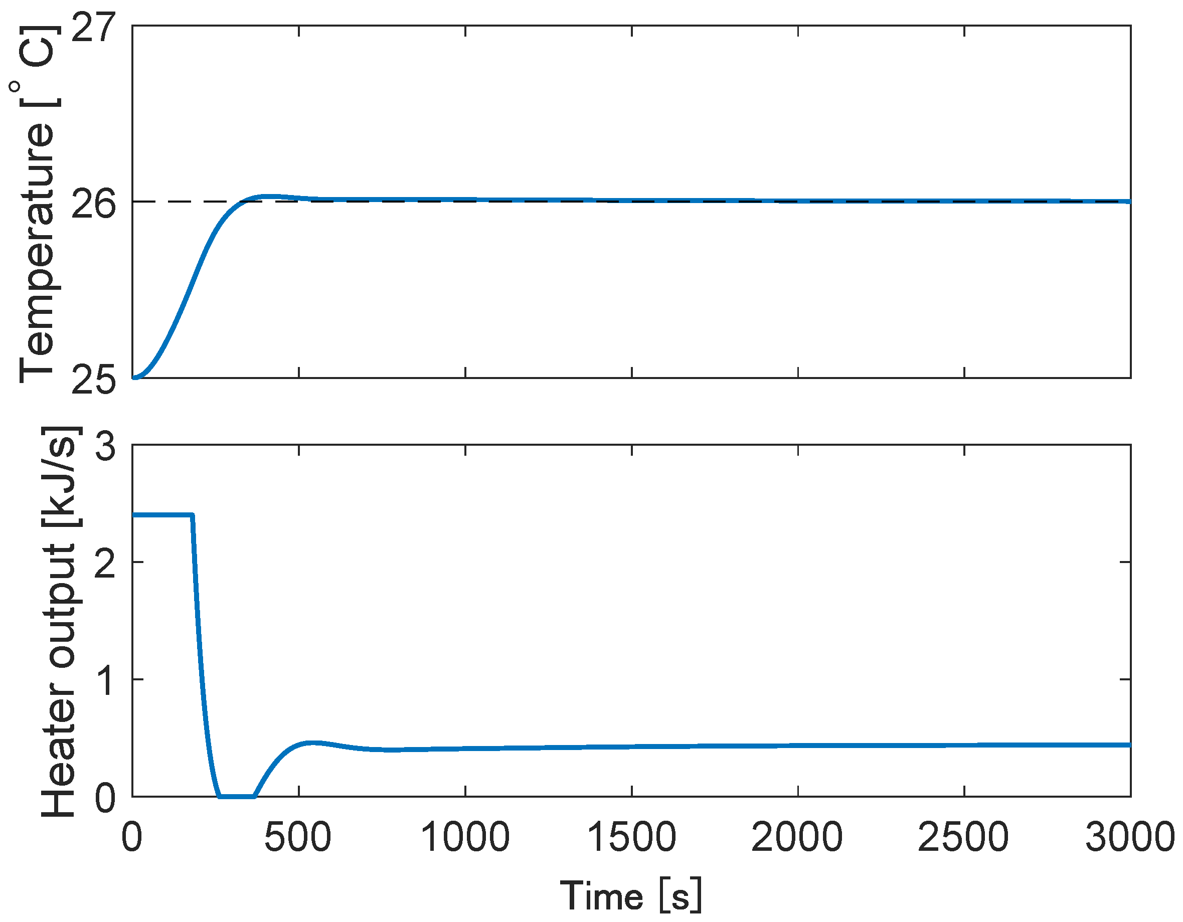
5.1. Simulation Results

This section presents the simulation results of the proposed control system. The simulation results were obtained using MATLAB R2023a(MATLAB9.14), which is one of the most effective software products for system engineering. The simulation parameters are shown in

Table 2. Simulation parameters.

Parameter	Definition	Value
	Simulation time	3500 s
	Sampling time	$1.0$ s
$r_w$	Target liquid level	40 $\mathrm{cm}$
$r_t$	Target liquid temperature	26 ${}^{\circ }\mathrm{C}$
$y_{w_0}$	Initial value	35 $\mathrm{cm}$
$y_{t_0}$	Initial value	25 ${}^{\circ }\mathrm{C}$
$K_{P_t}$	Proportional gain	3.0
$K_{I_t}$	Integral gain	0.0015
$K_{P_w}$	Proportional gain	1.0
$K_{I_w}$	Integral gain	0.003
$K_{P_{tw}}$	Proportional gain	50
$K_{I_{tw}}$	Integral gain	0.02
p	Differential factorial	$0.95$
q	Differential factorial	$1.05$
$q_w$	Differential factorial	$5/14$
$G_1$	Gain	$0.001$
$G_2$	Gain	$0.0005$
${\omega }_1$	Angular frequency	$\pi /30$ $\mathrm{rad}/\mathrm{s}$
${\omega }_2$	Angular frequency	$3\pi /4$ $\mathrm{rad}/\mathrm{s}$

and the simulation results of the proposed control system are shown in Figure 7 and Figure 8. A control parameter that generates a slight overshoot for ${\theta }_2$ was set, and the overshoot was reduced by pumping liquid. From Figure 7 and Figure 8, it can be seen that the liquid flow rate increases when ${\theta }_2$ exceeds the target value and the cooling operation is performed. Finally, it can be seen that the liquid temperature and liquid level follow the target values.

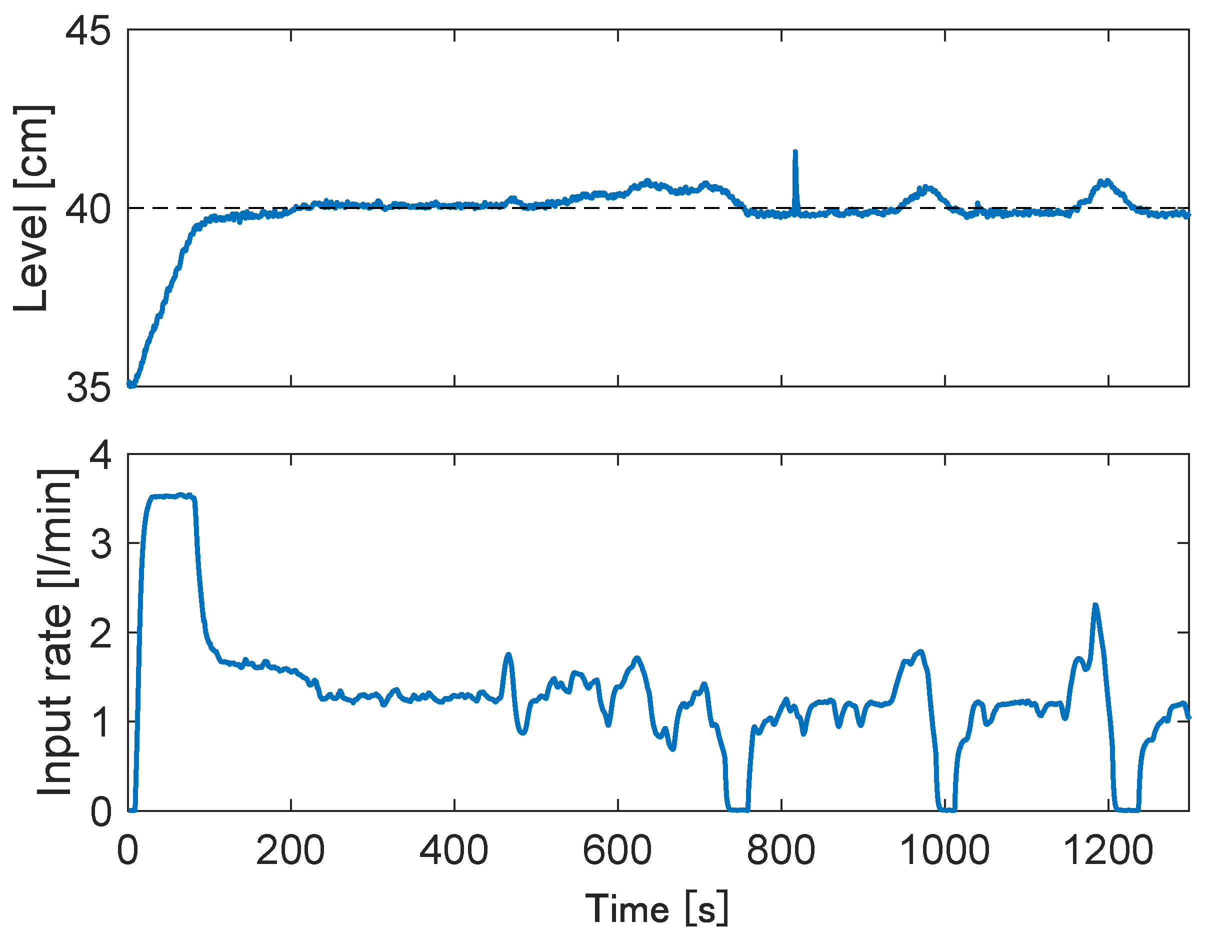
5.2. Exprimental Results

This section presents the results of experiments on the proposed control system using an actual device. Figure 9 and Figure 10 show the results of the experiment with the initial and target TANK2 liquid temperatures of 25 °C and 26 °C, respectively, and the initial and target TANK1 liquid levels of 35 cm and 40 cm, respectively. The parameters used in the experiments are shown in

Table 3. Expriment parameters.

Parameter	Definition	Value
	Sampling time	$1.0$ s
	Outside temperature	22 ${}^{\circ }\mathrm{C}$
$r_w$	Target liquid level	40 $\mathrm{cm}$
$r_t$	Target liquid temperature	26 ${}^{\circ }\mathrm{C}$
$y_{w_0}$	Initial value	35 $\mathrm{cm}$
$y_{t_0}$	Initial value	25 ${}^{\circ }\mathrm{C}$
${\theta }_i$	Inflow liquid temperature	20 ${}^{\circ }\mathrm{C}$
$K_{P_t}$	Proportional gain	1.8
$K_{I_t}$	Integral gain	0.0024
$K_{P_w}$	Proportional gain	1.1
$K_{I_w}$	Integral gain	0.003
$K_{P_{tw}}$	Proportional gain	15
$K_{I_{tw}}$	Integral gain	0.001
p	Differential factorial	$1.1$
q	Differential factorial	$1.05$
$q_w$	Differential factorial	$5/14$
$G_1$	Gain	$0.001$
$G_2$	Gain	$0.0005$
${\omega }_1$	Angular frequency	$\pi /30$ $\mathrm{rad}/\mathrm{s}$
${\omega }_2$	Angular frequency	$3\pi /4$ $\mathrm{rad}/\mathrm{s}$

. Figure 9 and Figure 10 show that both liquid level and liquid temperature can follow the target values while performing cooling operation when ${\theta }_2$ exceeds the target value in the experiment just as in the simulation. When a slight overshoot occurs for ${\theta }_2$, it can be confirmed that the overshoot is reduced by pumping liquid. Both the liquid temperature and the liquid level are finally able to follow the target values.

6. Conclusions

In this paper, we proposed a control system that can simultaneously track and control liquid level and temperature for a multi-input/output dual-tank device expressed using fractional calculus, and confirmed its operation through simulations and experiments. First, by considering the heat balance when the liquid volume in TANK1 changes during the heat exchange process, we constructed a model that can reproduce the temperature drop caused by the inflow of low-temperature liquid. Next, we designed a control system that can simultaneously control the liquid temperature and liquid level. For the liquid temperature control, heating by a heater and the temperature decrease that results from pumping liquid were used as inputs. Furthermore, modeling by fractional calculus was confirmed to control multivariate nonlinearity, compensate for uncertainties, and eliminate coupling effects. In conclusion, the simulation and experimental results show the effectiveness of the multivariable fractional-order controller design for a nonlinear dual-tank device. Previous control methods cannot simultaneously control liquid temperature and liquid level, but in this paper, the model was designed with a variable liquid volume, so simultaneous control was possible in simulation and experiment. The settling time was reduced by 2500 s compared to the previous control method. No overshooting or undershooting occurred, and the system was found to be stable even after following the target value. As for future development, because this paper describes a control system design using fractional-order derivatives based on operator theory, it is possible to propose a control system that compensates for tracking using fractional-order derivatives for a tracking compensator as well. In addition, it is expected that the control system design for interference introduced in this paper can be improved by designing the control system as a fractional-order derivative.

References

1. Deng, M.; Iwai, Z.; Mizumoto, I. Robust parallel compensator design for output feedback stabilization of plants with structured uncertainty. Syst. Control. Lett. 1999, 36, 193–198. [Google Scholar] [CrossRef]
2. Shah, S.L.; Iwai, Z.; Mizumoto, I.; Deng, M. Simple adaptive control of processes with time-delay. J. Process. Control 1997, 7, 439–449. [Google Scholar] [CrossRef]
3. Matsumoto, K.; Saito, D.; Wakui, S. Comparison of Connection Methods of One-axis Tracking Filters and Implementation for Pneumatic Anti-Vibration Apparatus. In Proceedings of the 2018 International Conference on Advanced Mechatronic Systems, Zhengzhou, China, 29 August–2 September 2018. [Google Scholar]
4. Ishii, H.; Wakui, S. Performance improvement of PDD2 compensator embedded in position control for pneumatic stage. In Proceedings of the 2019 International Conference on Advanced Mechatronic Systems, Kusatsu, Japan, 26–28 August 2019. [Google Scholar]
5. Patra, A.K.; Nanda, A. Automated micro insulin dispenser system based on the model predictive control algorithm. Int. J. Adv. Mechatron. Syst. 2020, 8, 144–154. [Google Scholar] [CrossRef]
6. Wen, S.; Liang, T.; Wang, P. Adaptive position estimation and control for permanent magnet synchronous motor. In Proceedings of the 2018 International Conference on Advanced Mechatronic Systems, Zhengzhou, China, 29 August–2 September 2018. [Google Scholar]
7. Shafieenejad, I. Novel method for bang-bang optimal control of starship soft landing. Int. J. Adv. Mechatron. Syst. 2023, 10, 146–155. [Google Scholar] [CrossRef]
8. Wang, C.; Man, Z.; Jin, J.; Ye, W. Hash-Based Convolutional Deep-thinking Pattern Classifier. In Proceedings of the 2023 International Conference on Advanced Mechatronic Systems, Melbourne, Australia, 4–7 September 2023. [Google Scholar]
9. Cheng, W.; Liu, T.; Liang, S. Temperatrue Control of Microwave Heating System by Adaptive Dynamic Programming. In Proceedings of the 2020 International Conference on Advanced Mechatronic Systems, Hanoi, Vietnam, 10–13 December 2020. [Google Scholar]
10. Rsetam, K.; Cao, Z.; Man, Z. Design of Robust Terminal Sliding Mode Control for Underactuated Flexible Joint Robot. IEEE Trans. Syst. Man Cybern. Syst. 2022, 52, 4272–4285. [Google Scholar] [CrossRef]
11. Man, Z.; Paplinski, A.P.; Wu, H.R. A robust MIMO terminal sliding mode control scheme for rigid robotic manipulators. IEEE Trans. Autom. Control 1994, 39, 2464–2469. [Google Scholar]
12. Wang, H.; Man, Z.; Kong, H.; Zhao, Y.; Yu, M.; Cao, Z.; Zheng, J.; Do, M.T. Design and Implementation of Adaptive Terminal Sliding-Mode Control on a Steer-by-Wire Equipped Road Vehicle. IEEE Trans. Ind. Electron. 2016, 63, 5774–5785. [Google Scholar] [CrossRef]
13. Yu, X.; Man, Z. Model reference adaptive control systems with terminal sliding modes. Int. J. Control 1996, 64, 1165–1176. [Google Scholar] [CrossRef]
14. Chen, J.; Qian, D. Three controllers via 2nd-order sliding mode for leader-following formation control of multi-robot systems. Int. J. Adv. Mechatron. Syst. 2021, 9, 85–101. [Google Scholar] [CrossRef]
15. Deng, M. Operator-Based Nonlinear Control Systems: Design and Applications; John Wiley & Sons: Hoboken, NJ, USA, 2014; pp. 5–26. [Google Scholar]
16. Chen, G.; Han, Z. Robust right coprime factorization and robust stabilization of nonlinear feedback control systems. IEEE Trans. Autom. Control 1998, 43, 1505–1509. [Google Scholar] [CrossRef]
17. Gao, X.; Yang, Q.; Zhang, J. Multi-objective optimisation for operator-based robust nonlinear control design for wireless power transfer systems. Int. J. Adv. Mechatron. Syst. 2022, 9, 203–210. [Google Scholar] [CrossRef]
18. Bu, N.; Zhang, Y.; Li, X. Robust tracking control for uncertain micro-hand actuator with Prandtl-Ishlinskii hysteresis. Int. J. Robust Nonlinear Control 2023, 33, 9391–9405. [Google Scholar] [CrossRef]
19. Bu, N.; Liu, H.; Li, W. Robust passive tracking control for an uncertain soft actuator using robust right coprime factorization. Int. J. Robust Nonlinear Control 2021, 31, 6810–6825. [Google Scholar] [CrossRef]
20. Bu, N.; Wang, X. Swing-up design of double inverted pendulum by using passive control method based on operator theory. Int. J. Adv. Mechatron. Syst. 2023, 10, 1–7. [Google Scholar] [CrossRef]
21. Wang, A.; Deng, M. Robust nonlinear multivariable tracking control design to a manipulator with unknown uncertainties using operator-based robust right coprime factorization. Trans. Inst. Meas. Control 2013, 35, 788–797. [Google Scholar] [CrossRef]
22. Deng, M.; Inoue, A.; Goto, S. Operator based thermal control of an aluminum plate with a peltier device. Int. J. Innov. Comput. Inf. Control 2008, 4, 3219–3229. [Google Scholar]
23. Furukawa, K.; Deng, M. Operator based fault detection and compensation design of an unknown multivariable tank process. In Proceedings of the 2013 International Conference on Advanced Mechatronic Systems, Luoyang, China, 25–27 September 2013. [Google Scholar]
24. Keith, B.O.; Jerome, S. The Fractional Calculus; Dover Publications: Mineola, NY, USA, 2006; pp. 107–117. [Google Scholar]
25. Das, S. Functional Fractional Calculus; Springer: Berlin/Heidelberg, Germany, 2011; pp. 149–152. [Google Scholar]
26. Fractional Calculus: What Is It? Available online: https://igor.podlubny.website.tuke.sk/fc.html (accessed on 24 December 2023).
27. Zhang, T.; Li, Y. Exponential Euler scheme of multi-delay Caputo-Fabrizio fractional-order differential equations. Appl. Math. Lett. 2022, 124, 107709. [Google Scholar] [CrossRef]
28. Nasuno, H.; Shimizu, N. Numerical Integration Algorithm for Nonlinear Fractional Differential Equation. Trans. Jpn. Soc. Mech. Eng. Ser. C 2006, 72, 3193–3200. [Google Scholar] [CrossRef]
29. Mehta, U.; Aryan, P.; Raja, G.L. Tri-Parametric Fractional-Order Controller Design for Integrating Systems with Time Delay. IEEE Trans. Circuits Syst. II Express Briefs 2023, 70, 4166–4170. [Google Scholar] [CrossRef]
30. Arya, Y. A new optimized fuzzy FOPI-FOPD controller for automatic generation control of electric power systems. J. Frankl. Inst. 2019, 356, 16–32. [Google Scholar] [CrossRef]
Figure 1. Cross-section of tank device.
Fractalfract 08 00027 g001
Figure 2. Tank heat balance.
Fractalfract 08 00027 g002
Figure 3. Proposed control system.
Fractalfract 08 00027 g003
Figure 4. Uncertainty compensation.
Fractalfract 08 00027 g004
Figure 5. Elimination of coupling effects.
Fractalfract 08 00027 g005
Figure 6. Details of the proposed control system.
Fractalfract 08 00027 g006
Figure 7. Simulation results: liquid temperature and heater output. The dotted line is reference temperature.
Fractalfract 08 00027 g007
Figure 8. Simulation results: liquid level and input rate. The dotted line is reference water level.
Fractalfract 08 00027 g008
Figure 9. Experimental results: liquid temperature and heater output. The dotted line is reference temperature.
Fractalfract 08 00027 g009
Figure 10. Experimental results: liquid level and input rate. The dotted line is reference water level.
Fractalfract 08 00027 g010