Global Stability of Fractional Order HIV/AIDS Epidemic Model under Caputo Operator and Its Computational Modeling

Abstract

The human immunodeficiency virus (HIV) causes acquired immunodeficiency syndrome (AIDS), which is a chronic and sometimes fatal illness. HIV reduces an individual’s capability against infection and illness by demolishing his or her immunity. This paper presents a new model that governs the dynamical behavior of HIV/AIDS by integrating new compartments, i.e., the treatment class T. The steady-state solutions of the model are investigated, and accordingly, the threshold quantity $R_0$ is calculated, which describes the global dynamics of the proposed model. It is proved that for $R_0$ less than one, the infection-free state of the model is globally asymptotically stable. However, as the threshold number increases by one, the endemic equilibrium becomes globally asymptotically stable, and in such case, the disease-free state is unstable. At the end of the paper, the analytic conclusions obtained from the analysis of the ordinary differential equation (ODE) model are supported through numerical simulations. The paper also addresses a comprehensive analysis of a fractional-order HIV model utilizing the Caputo fractional differential operator. The model’s qualitative analysis is investigated, and computational modeling is used to examine the system’s long-term behavior. The existence/uniqueness of the solution to the model is determined by applying some results from the fixed points of the theory. The stability results for the system are established by incorporating the Ulam–Hyers method. For numerical treatment and simulations, we apply Newton’s polynomial and the Toufik–Atangana numerical method. Results demonstrate the effectiveness of the fractional-order approach in capturing the dynamics of the HIV/AIDS epidemic and provide valuable insights for designing effective control strategies.

1. Introduction

AIDs is a sexually transmitted infection that impairs the routine functions of an individual immune response to a disease. The disease spreads through HIV, which destroys an individual’s ability to withstand infections. In 1981, the foremost AIDS case was reported, and since then, HIV has constantly been spreading around the globe. In 2009, about 20 individuals perished globally, and the disease is still endemic [1]. Consequently, some genuine antiviral medications are needed to decrease these deaths [1,2]. There are several barriers to HIV/AIDS medication due to the lack of a vaccine. The modern HIV/AIDS treatment consists of administering two or even more drugs at the same time, and usually, these drugs are from the two primary groups: protease inhibitors (PIs) and reverse transcriptase inhibitors (RTIs) [3,4]. By taking antiretroviral medication, patients can increase their lifespan by extending the time that they are free of HIV complications. Individuals with HIV who agree to medication before developing AIDS can considerably lower the danger of transfer of the disease to upcoming generations [5,6]. According to reports, mother-to-child propagation accounts for $40\%$ of all HIV/AIDS infections, and in 1997, fewer than 300 newborns in the United States contracted HIV via vertical routes. AIDS killed about $2.5$ millions youngsters below the age of 15 in sub-Saharan Africa. The majority of these youngsters were infected with HIV during delivery or nursing. That is why the early detection and treatment of AIDS is critical and urgent [7,8].

Contiguous diseases may be studied very well with the aid of mathematical models. In Ref. [9], Yusuf and Benyah provided and analyzed an ODE model for limiting the increase in HIV/AIDS cases, utilizing the variations in sexual behavior and antiviral (ARV) medication as control policies, and estimated the system’ parameters and states value using the reported cases of the South African demographic. The findings of the study indicate that the efficient strategy to restrict the transmission of HIV/AIDS is for vulnerable persons to engage himself/herself in safer sexual practices as much as they can, and the ARV medications should be administered to those persons who have not yet reached the severe conditions of AIDS. Huo and Feng [10] investigated an epidemic model for AIDS having slow and rapid latency classes, and it was found that it is highly important to treat people in the fast and slow classes in order to control the spread. For more details on the dynamical behavior of HIV/AIDS and other related epidemics, the readers are advised to see [11,12,13,14,15,16,17,18] and the reference materials cited therein.

Inspired by the preceding research works, we investigate a basic HIV/AIDS pandemic model, including therapy, in this study. From the previous literature, a novel model for HIV/AIDS epidemic is formulated by adding the treatment class T. People in class T are subjected to a variety of therapies. These medications do not entirely remove HIV from the human body. Even in the case of an effective treatment, the virus is suppressed to extremely low levels. Those individuals who are suffering from HIV, after the treatment, can live longer and better lives by reducing the quantity of viruses in their body. However, after the treatment, they can still spread the virus, and they must take antiviral medications on a regular basis to maintain their health. The resident of class T will move to the class of HIV-positive individuals at the phase of HIV infection (I) or full-blown AIDS not receiving ARV therapy $\left(A\right)$ if the medication is failed or canceled. Our primary objective in this work is to explore the relative effect of treatment on the dynamical aspects of HIV/AIDS.

Ordinary and partial differential equations, and stochastic and delay differential equations are the most often used methodologies for modeling epidemics. There have been a lot of studies on mathematical models for infectious illnesses that take into account fractional and fractal-fractional operators, for example, see [19,20,21]. A fractional modeling technique was also used here in this paper to investigate the dynamics of the new AIDS model. The dynamic processes are represented as a set of differential equations having a fractional-order Caputo derivative. Parallel to the simulation analysis, a full theoretical examination of the fractional scenario is completed. The existence/uniqueness of the model’s solution are determined by applying some theorem of the fixed points. The analysis of the stability of the system is established by incorporating the Ulam–Hyers method. Lastly, we present a simulation studies of the problem using Newton’s polynomial and the Toufik–Atangana numerical approach, as well as a sketch of the influence of key crucial parameters of the proposed system on the dynamic behaviors of HIV/AIDS. The remaining parts of the manuscript are structured as follows. In Section 2, we formulate the ODE model and present the basic properties of the underlying model. The model analysis, along with stability analysis, is carried out in Section 3. Section 4 introduces the fractional-order model and some fundamental ideas of the fractional derivative. Section 5 illustrates the comprehensive theoretical study of the fractional model, which covers the existence/uniqueness and stability analyses. Section 6 outlines the numerical process for obtaining the numerical solution of the system and, using graphs, gives some deep insights into the influence of various parameters. Section 7 discusses the numerical scheme and simulations related to the study. Section 8 concludes the study with some practical advice on the dynamical aspects of the epidemic HIV/AIDS.

2. Structure of the Model

This section introduces a simplified model describing the dynamical behaviors of HIV and AIDS, particularly showing the impact of treatment. To formulate the compartmental model, let us assume that the entire population is stratified into five disjoint groups, namely, $S\left(t\right)$ is the class of vulnerable people; $I\left(t\right)$ stands for the number of positive HIV cases within the stage of HIV; the number of people with full-blown AIDS who are not receiving ARV therapy is denoted by $A\left(t\right)$; the individuals under treatment are described as $T\left(t\right)$; and $R\left(t\right)$ indicates the total number of individuals who have modified their sexual practices substantially to be resistant to HIV transmission through sexual relations. It is also assumed that a vulnerable person may become infected by coming into touch with contagious people. Despite AIDS not being a curable disease, therapy is extremely vital. As a result, in this study, we undertake studies on the medication of HIV patients. Upon treatment, the likelihood of persons developing AIDS is reduced, as is the chance of passing the disease on to subsequent generations. Here, by $R\left(t\right)$, we do not mean fully recovered; in fact, it denotes those individuals who adopt safe sexual behaviors and stick with them for the entire duration of their life spans [9]. The change in these individual compartments is mathematically described by the following set of equations:

$$\begin{array}{cc}\hfill & \frac{dS\left(t\right)}{dt}=-\beta S\left(t\right)I\left(t\right)+\Lambda -dS\left(t\right)-{\mu }_{1}S\left(t\right),\hfill \\ \hfill & \frac{dI\left(t\right)}{dt}=\beta I\left(t\right)S\left(t\right)-dI\left(t\right)+{\alpha }_{1}T\left(t\right)-k_{2}I\left(t\right)-k_{1}I\left(t\right),\hfill \\ \hfill & \frac{dA\left(t\right)}{dt}=k_{1}I\left(t\right)+{\alpha }_{2}T-\left(d+{\delta }_1\right)A,\hfill \\ \hfill & \frac{dT\left(t\right)}{dt}=k_{2}I\left(t\right)-{\alpha }_{1}T\left(t\right)-\left(d+{\delta }_2+{\alpha }_2\right)T\left(t\right),\hfill \\ \hfill & \frac{dR\left(t\right)}{dt}={\mu }_{1}S\left(t\right)-dR\left(t\right).\hfill \end{array}$$

(1)

We suppose that each of the model’s parameters is positive and constant. The parameters $\Lambda ,d$ and $\beta$ respectively denote the rate of recruitment into the susceptible population, natural death rates in each class, and the rate at which the infected individuals make contact with the susceptible people. The parameter $k_1$ is the pace at which people leave the infectious group and contract full-blown AIDS; it is the fraction of the I that develops full-blown AIDS. The infection also causes deaths in the infected compartments and, respectively, ${\delta }_i$’s for $i=1,2$ are the infection-related mortality rates in the classes A and T. The rate of treatment in the HIV-infected compartment is denoted by $k_2$ and in a unit time; it is proportional to the class I, which is individuals under treatment. It implies that not everyone accepts therapy, and that some individuals refuse treatment due to financial constraints. Raising the rate of therapy is critical for eliminating HIV/AIDS. The pace at which vulnerable people alter their sexual practices per given period of time is denoted by ${\mu }_1$. The removal rate from class $T\left(t\right)$ is given by ${\alpha }_1$, and for the sake of simplicity, the description, value, units and source of parameters are presented in

Table 1. Parameters description, values, units and sources used in model (1).

Parameters	The Physical Interpretation	Value	Date Source
$\Lambda$	The rate at which people are entering into the susceptible class	0.55 year−1	[10]
d	Natural mortality rate	0.0196 year−1	[9]
$\beta$	Transmitting coefficient of the disease phase	0.03 year−1	Estimate
$k_2$	The rate at which people moves form class I to T	0.35 year−1	Estimate
${\alpha }_2$	Denotes the fraction of people with fail treatment	Variable
${\alpha }_1$	Denotes the fraction of people with full treatment	Variable
$k_1$	The rate at which people moves form class A to I	0.15 year−1	Estimate
${\delta }_1$	AIDS-induced mortality rate	0.0909 year−1	[9]
${\mu }_1$	Percentage of vulnerable people who modified their behaviors	0.03 year−1	[9]
${\delta }_2$	Mortality rate in the treatment compartment due to the infection	0.0667 year−1	[9]

.

3. Deterministic System (1) and Its Analysis

In the present part of the manuscript, we analyze the deterministic model (1), and we take help from [22,23,24,25].

3.1. Positivity of Solutions

Lemma 1.

Any solution $(S,I,A,R,T)\left(t\right)$ of model (1) with a given initial data $S\left(0\right)>0, A\left(0\right)\ge 0, I\left(0\right)\ge 0, T\left(0\right)\ge 0, R\left(0\right)\ge 0$ is non-negative for each $0<t$.

Proof. 

Keeping in view the work of Sharomi and Podder [14], the first equation in model (1) can be expressed alternatively as

$$\frac{d}{dt}\left[exp\left\{{\int }_0^t\beta I\left(\tau \right)d\tau +\left(d+{\mu }_1\right)t\right\}S\left(t\right)\right]=\Lambda exp\left\{{\int }_0^t\beta I\left(\tau \right)d\tau +\left(d+{\mu }_1\right)t\right\}.$$

(2)

Thus,

$$S\left(t_1\right)exp\left\{{\int }_0^{t_1}I\left(\tau \right)\beta d\tau +\left(d+{\mu }_1\right)t_1\right\}-S\left(0\right)={\int }_0^{t_1}\Lambda exp\left\{{\int }_0^{y}I\left(\tau \right)\beta d\tau +\left(d+{\mu }_1\right)y\right\}dy,$$

(3)

from which we can write

$$\begin{array}{cc}\hfill S\left(t_1\right)=& S\left(0\right)exp\left\{-{\int }_0^{t_1}I\left(\tau \right)\beta d\tau -\left(d+{\mu }_1\right)t_1\right\}\hfill \\ \hfill & +exp\left\{-{\int }_0^{t_1}I\left(\tau \right)\beta d\tau -\left(d+{\mu }_1\right)t_1\right\}\times {\int }_0^{t_1}\Lambda exp\left\{{\int }_0^{y}I\left(\tau \right)\beta d\tau +\left(d+{\mu }_1\right)y\right\}dy>0.\hfill \end{array}$$

(4)

In the same way, one can easily prove that $A\left(t\right)\ge 0, I\left(t\right)\ge 0, R\left(t\right)\ge 0, T\left(t\right)\ge 0$. Therefore, any solution $(S,I,A,R,T)\left(t\right)$ of model (1) with given non-negative initial data is positive for each $0<t$. □

3.2. The Invariant Region

Lemma 2.

The region of feasibility Ω for the problem under consideration is defined by

$$\Omega =\left\{(S,I,A,T,R)\left(t\right)\in R_{+}^5\mid \frac{\Lambda }{d}\ge S+I+A+T+R\ge 0\right\},$$

(5)

where $R_{+}^5$ stands for the positive cone of $R_{+}^5$, and the lower-dimensional face is the positive invariant set for model (32) with any initial conditions in $R_{+}^5$.

Proof. 

By adding all of the equations of model (1), we have

$$\frac{dN}{dt}=-{\delta }_{2}T+\Lambda -{\delta }_{1}A-dN\le -dN+\Lambda .$$

(6)

Upon solving this differential inequality, we obtain the following:

$$e^{-dt}N\left(0\right)+\frac{\Lambda }{d}\ge N\left(t\right),$$

(7)

where $N\left(0\right)$ stands for the value of the total population at $t=0$. Thus, by applying the limit, we have ${lim}_{t\to \infty }supN\left(t\right)\le \frac{\Lambda }{d}$. Further, from the previous lemma, we have $N\left(t\right)\ge 0$ for all time t. Hence, one can conclude that the set (5) is positive invariant for model (1). □

3.3. The Disease-Free State and Derivation of $R_0$

Following the steady-state case of the proposed system, one can easily prove that model (1) has always an infection-free state, which is given by

$$E_0=\left(\frac{\Lambda }{d+{\mu }_1},0,0,0,\frac{{\mu }_1\Lambda }{\left({\mu }_1+d\right)d}\right).$$

(8)

Following the well-known method of the next generation matrix [22,23], one can obtain the threshold quantity $R_0$ for the underlying model. To proceed further, let us re-arrange system (1) in the following form:

$$\begin{array}{cc}\hfill \frac{dI}{dt}& ={\alpha }_{1}T+\beta IS-dI-k_{2}I-k_{1}I,\hfill \\ \hfill \frac{dA}{dt}& =-\left(d+{\delta }_1\right)A+k_{1}I+{\alpha }_{2}T,\hfill \\ \hfill \frac{dT}{dt}& =-{\alpha }_{1}T+k_{2}I-\left({\alpha }_2+d+{\delta }_2\right)T,\hfill \\ \hfill \frac{dS}{dt}& =\Lambda -{\mu }_{1}S-\beta IS-dS,\hfill \\ \hfill \frac{dR}{dt}& =-dR+{\mu }_{1}S.\hfill \end{array}$$

(9)

Assume that $z={(I,A,T,S,R)}^T$, then model (9) will take the form

$$\frac{dz}{dt}=\mathcal{W}\left(z\right)-\mathcal{U}\left(z\right),$$

(10)

where,

$$\mathcal{W}\left(z\right)=\left(\begin{array}{c}\beta IS\\ 0\\ 0\\ 0\\ 0\end{array}\right),\mathcal{U}\left(z\right)=\left(\begin{array}{c}\left(k_1+k_2+d\right)I-{\alpha }_{1}T\\ \left({\delta }_1+d\right)A-k_{1}I-{\alpha }_{2}T\\ \left(d+{\delta }_2+{\alpha }_2+{\alpha }_1\right)T-k_{2}I\\ \beta IS+{\mu }_{1}S+dS-\Lambda \\ -{\mu }_{1}S+dR\end{array}\right).$$

(11)

We calculate the Jacobian of the matrices $\mathcal{W}\left(z\right)$ and $\mathcal{U}\left(z\right)$ at the infection-free states, which yields

$$D\mathcal{W}\left(E_0\right)=\left(\begin{array}{ccc}{F}_{3\times 3}& 0& 0\\ 0& 0& 0\\ 0& 0& 0\end{array}\right),D\mathcal{U}\left(E_0\right)=\left(\begin{array}{cccc}{V}_{3\times 3}& 0& & 0\\ \beta \frac{\Lambda }{{\mu }_1+d}& 0& 0& d+{\mu }_1& 0\\ 0& 0& 0& -{\mu }_1& d\end{array}\right),$$

(12)

where

$$W_{3\times 3}=\left(\begin{array}{ccc}\beta \frac{\Lambda }{{\mu }_1+d}& 0& 0\\ 0& 0& 0\\ 0& 0& 0\end{array}\right),U_{3\times 3}=\left(\begin{array}{ccc}{k}_2+k_1+d& 0& -{\alpha }_1\\ -k_1& {\delta }_1+d& -{\alpha }_2\\ -k_2& 0& {\delta }_2+d+{\alpha }_2+{\alpha }_1\end{array}\right).$$

(13)

The threshold parameter $R_0$ can be written as

$$\begin{array}{cc}\hfill R_0& =\rho \left(W{U}^{-1}\right)=\frac{\beta \left({\delta }_2+d+{\alpha }_1+{\alpha }_2\right)\Lambda }{\left(k_1+k_2+d\right)\left({\delta }_2+d+{\alpha }_2+{\alpha }_1\right)\left(d+{\mu }_1\right)-k_2{\alpha }_1\left(d+{\mu }_1\right)}\hfill \\ \hfill & =\frac{\beta \Lambda }{\left(k_2+k_1+d\right)\left(d+{\mu }_1\right)-\frac{k_2{\alpha }_1\left(d+{\mu }_1\right)}{{\delta }_2+d+{\alpha }_2+{\alpha }_1}}.\hfill \end{array}$$

(14)

3.4. Global Stability Analysis of $E^0$

Theorem 1.

The infection-free state $E^0$ of system (1) is globally asymptotically stable whenever $R_0$ is less than one.

Proof. 

Following the ideas of Cheng et al. [24] and Li and Jin [25], we consider the Lyapunov function:

$$V\left(t\right)=mT+I,0<m.$$

(15)

By assuming the derivative of (15) w.r.t. time, we have

$$\frac{dV}{dt}=\frac{dI}{dt}+m\frac{dT}{dt}.$$

(16)

By putting values of $\frac{I}{dt}$ and $\frac{T}{dt}$ from the model into Equation (16), we have

$$\frac{dV}{dt}={\alpha }_{1}T+\beta IS-dI-k_{2}I-k_{1}I+m\left[-{\alpha }_{1}T+k_{2}I-\left({\alpha }_2+d+{\delta }_2\right)T\right].$$

(17)

Keeping in view the values of S and R from the disease-free states, that is, $S_0=\Lambda /\left({\mu }_1+d\right)$ and ${\overline{R}}_0=\Lambda {\mu }_1/\left({\mu }_1+d\right)d$, (17) will take the form

$$\dot{V}+{\alpha }_1\le \left[\frac{\beta \Lambda }{\left({\mu }_1+d\right)}-\left(k_2+d+k_1\right)+k_{2}m\right]I\left(t\right)+T\left(t\right)\left[-m\left(d+{\alpha }_2+{\delta }_2+{\alpha }_1\right)\right].$$

(18)

If we chose $m=\frac{{\alpha }_1}{d+{\alpha }_2+{\delta }_2+{\alpha }_1}$, one can write the above inequality as

$$\begin{array}{cc}\hfill \frac{dV}{dt}& \le \left[\frac{\beta \Lambda }{\left({\mu }_1+d\right)}-\left(k_2+d+k_1\right)+\frac{k_2{\alpha }_1}{{\delta }_2+d+{\alpha }_2+{\alpha }_1}\right]I,\hfill \\ \hfill & =\frac{\beta \Lambda \left(d+{\alpha }_2+{\delta }_2+{\alpha }_1\right)-\left(k_2+d+k_1\right)\left(d+{\alpha }_2+{\delta }_2+{\alpha }_1\right)\left(d+{\mu }_1\right)+k_2{\alpha }_1\left(d+{\mu }_1\right)}{\left(d+{\mu }_1\right)\left({\alpha }_2+{\delta }_2+d+{\alpha }_1\right)}I.\hfill \end{array}$$

(19)

Since

$$\begin{array}{cc}\hfill -1+R_0& =\frac{\beta \Lambda \left({\alpha }_1+{\delta }_2+d+{\alpha }_2\right)-\left(k_2+d+k_1\right)\left({\delta }_2+d+{\alpha }_2+{\alpha }_1\right)\left({\mu }_1+d\right)+k_2{\alpha }_1\left(d+{\mu }_1\right)}{\left(d+{\mu }_1\right)\left({\alpha }_2+{\delta }_2+d+{\alpha }_1\right)\left(k_2+d+k_1-k_2{\alpha }_1\right)},\hfill \\ \hfill \frac{dV}{dt}& \le \frac{\left(R_0-1\right)\left[\left(k_2+d+k_1\right)\left({\alpha }_2+{\delta }_2+d+{\alpha }_1\right)\left(d+{\mu }_1\right)-k_2{\alpha }_1\left(d+{\mu }_1\right)\right]}{\left(d+{\mu }_1\right)\left({\alpha }_2+{\delta }_2+d+{\alpha }_1\right)}I,\hfill \\ \hfill & =\frac{\left(R_0-1\right)\left[\left(d+k_1+k_2\right)\left({\alpha }_2+{\delta }_2+d+{\alpha }_1\right)-{\alpha }_1{k}_2\right]}{{\alpha }_1+d+{\delta }_2+{\alpha }_2}I\le 0.\hfill \end{array}$$

(20)

It is to be noted that $\frac{dV}{dt}=0$ only if $T=I=0$. By letting $T=I=0$ in model (1), one can arrive at the conclusion that

$$S\to \frac{\Lambda }{\left(d+{\mu }_1\right)},A\to 0\mathrm{and}R\to \frac{\Lambda {\mu }_1}{\left(d+{\mu }_1\right)d},$$

as t approaches ∞. Following LaSalle’s principle of invariance [26], we conclude that the infection-free state of the system is globally asymptotically stable.

LaSalle’s principle of invariance is an essential concept in the study of dynamical systems. It states that, within a certain region of the state space, trajectories of a dynamical system will converge to a set known as the “invariant set”. This set contains points where the derivative of the Lyapunov function is zero, implying that the system’s behavior becomes bounded over time. In our analysis, invoking this principle allows us to conclude that the infection-free state is globally asymptotically stable. This, in turn, signifies that any initial condition within a specific region of the state space will ultimately tend toward the infection-free state as time progresses. □

3.5. Existence of the Endemic Equilibrium

In the previous part of the study, we investigated that for $R_0<1$, the infection tends to eliminate out of the population. However, for $R_0>1$, there exists a unique endemic state of system (1) that is given by $E^{*}=\left(S^{*},I^{*},A^{*},T^{*},R^{*}\right)$, where

$$\begin{array}{cc}\hfill S^{*}& =\frac{\Lambda }{{\mu }_1+\beta I^{*}+d},\hfill \\ \hfill I^{*}& =\frac{1}{\beta }\left(-1+R_0\right)\left(d+{\mu }_1\right),\hfill \\ \hfill A^{*}& =\frac{{\alpha }_2{T}^{*}+k_1{I}^{*}}{{\delta }_1+d}\hfill \\ \hfill T^{*}& =\frac{I^{*}{k}_2}{{\alpha }_2+{\delta }_2+d+{\alpha }_1},\hfill \\ \hfill R^{*}& =\frac{{\mu }_1\Lambda }{\left(\beta I^{*}+{\mu }_1+d\right)d}.\hfill \end{array}$$

(21)

3.6. Global Stability of the Endemic Equilibrium

Theorem 2.

The endemic state $E^{*}$ of system (1) is globally asymptotically stable whenever $R_0$ is greater than one.

Proof. 

Under the condition of $R_0>1$, we see that the system has one and only one steady state $E^{*}$. Now here, we intend to investigate the global analysis of this equilibrium. To do so, we consider the Lyapunov function V in the following form [27,28]:

$$V=-S^{*}lnS+S+\left(-I^{*}lnI+I\right)B+\left(-T^{*}lnT+T\right)D.$$

(22)

The time derivative of the above function V can be expressed as

$$\begin{array}{cc}\hfill \frac{dV}{dt}=& \left(-\frac{S^{*}}{S}+1\right)\frac{dS}{dt}+\left(-\frac{I^{*}}{I}+1\right)B\frac{dI}{dt}+\left(-\frac{T^{*}}{T}+1\right)D\frac{dT}{dt},\hfill \\ \hfill =& \left(1-\frac{S^{*}}{S}\right)\left(\Lambda -{\mu }_{1}S-\beta IS-dS\right)+\left(1-\frac{I^{*}}{I}\right)B\left({\alpha }_{1}T+\beta IS-dT-k_{2}I-k_{1}I\right)\hfill \\ \hfill & +\left(1-\frac{T^{*}}{T}\right)D\left[-{\alpha }_{1}T+k_{2}I-{\alpha }_{2}T-\left({\delta }_2+d\right)T\right],\hfill \\ \hfill =& \left(1-\frac{S^{*}}{S}\right)\left({\mu }_1{S}^{*}+\beta I^{*}{S}^{*}-\beta IS+d{S}^{*}-dS-{\mu }_{1}S\right)+\left(1-\frac{I^{*}}{I}\right)B\left({\alpha }_{1}T+\beta IS-\frac{\beta I^{*}{S}^{*}+{\alpha }_1{T}^{*}}{I^{*}}I\right)\hfill \\ \hfill & +\left(1-\frac{T^{*}}{T}\right)D\left(-k_2\frac{I^{*}}{T^{*}}T+k_{2}I\right).\hfill \end{array}$$

(23)

Now, let us suppose that

$$\frac{S}{S^{*}}=x,\frac{I}{I^{*}}=y,\frac{T}{T^{*}}=\mu ,$$

(24)

then Equation (23) takes the form

$$\begin{array}{cc}\hfill \frac{dV}{dt}=& \left(1-x^{-1}\right)\left({\mu }_1{S}^{*}+\beta I^{*}{S}^{*}-\beta S^{*}x{I}^{*}y+d{S}^{*}-{\mu }_{1}x{S}^{*}-x{S}^{*}d\right)\hfill \\ \hfill & +\left(1-\frac{1}{y}\right)B\left(\beta x{S}^{*}y{I}^{*}+\mu {\alpha }_1{T}^{*}-\frac{{\alpha }_1{T}^{*}+\beta I^{*}{S}^{*}}{I^{*}}y{I}^{*}\right)+\left(1-\frac{1}{\mu }\right)D\left(-k_2\frac{I^{*}}{T^{*}}{T}^{*}+k_2{I}^{*}y\right)\hfill \\ \hfill =& \left(1-x^{-1}\right)\left[\beta (1-yx)I^{*}{S}^{*}+{\mu }_1(1-x)S^{*}+d(1-x)S^{*}\right]\hfill \\ \hfill & +\left(1-y^{-1}\right)B\left[\beta (-y+xy)I^{*}{S}^{*}+{\alpha }_1(\mu -y)T^{*}\right]+\left(1-{\mu }^{-1}\right)D{k}_2(y-\mu )I^{*},\hfill \\ \hfill =& -\left({\mu }_1{S}^{*}+d{S}^{*}\right)\frac{{(-x+1)}^2}{x}+\left(1-\frac{1}{x}\right)I^{*}\beta S^{*}(-yx+1)\hfill \\ \hfill & +\left(1-y^{-1}\right)B\left[I^{*}\beta S^{*}(-y+yx)+T^{*}{\alpha }_1(-y+\mu )\right]+\left(1-\frac{1}{\mu }\right)D{I}^{*}{k}_2(-\mu +y),\hfill \\ \hfill =& -\left(d{S}^{*}+{\mu }_1{S}^{*}\right)\frac{{(-x+1)}^2}{x}+\beta S^{*}{I}^{*}\left(-yx+1-x^{-1}+y\right)+T^{*}{\alpha }_{1}B\left(-y+\mu +1-\frac{\mu }{y}\right)\hfill \\ \hfill & +B{S}^{*}\beta I^{*}(-x+yx+1-y)+I^{*}{k}_{2}D\left(-\frac{y}{\mu }-y+1-\mu \right),\hfill \\ \hfill =& -\left(d{S}^{*}+{\mu }_1{S}^{*}\right)\frac{{(-x+1)}^2}{x}+\left(S^{*}\beta I^{*}+I^{*}\beta B{S}^{*}+T^{*}{\alpha }_{1}B+I^{*}{k}_{2}D\right)\hfill \\ \hfill & +yx\left(I^{*}\beta B{S}^{*}-I^{*}\beta S^{*}\right)+\left(I^{*}\beta S^{*}-I^{*}\beta B{S}^{*}+I^{*}{k}_{2}D-T^{*}{\alpha }_{1}B\right)y\hfill \\ \hfill & +\left(T^{*}{\alpha }_{1}B-I^{*}{k}_{2}D\right)\mu -\beta \frac{S^{*}{I}^{*}}{x}-I^{*}\beta B{S}^{*}x-\frac{\mu }{y}B{\alpha }_1{T}^{*}-I^{*}{k}_{2}D\frac{y}{\mu }.\hfill \end{array}$$

(25)

The variables which occur in $\frac{dV}{dt}$ have non-negative coefficients $y,\mu$ and $yx$. If we prove that all of the coefficients of each term are positive, then we have that $\frac{dV}{dt}$ could also be positive. By setting equal to zero all of the coefficients of $y,\mu$ and $yx$, we obtain

$$B{I}^{*}\beta S^{*}-I^{*}\beta S^{*}=0,$$

(26)

$$T^{*}{\alpha }_{1}B-I^{*}{k}_{2}D=0,$$

(27)

and from Equations (26) and (27), we obtain

$$D=\frac{{\alpha }_1{T}^{*}}{k_2{I}^{*}},B=1.$$

(28)

Therefore, we can write

$$\begin{array}{cc}\hfill \frac{dV}{dt}& =-\left(d+{\mu }_1\right)S^{*}\frac{{(-x+1)}^2}{x}+2I^{*}\beta S^{*}+2T^{*}{\alpha }_1-\frac{S^{*}\beta I^{*}}{x}-S^{*}x\beta I^{*}-\frac{\mu }{y}{\alpha }_1{T}^{*}-T^{*}{\alpha }_1\frac{y}{\mu }\hfill \\ \hfill & =-\left(d{S}^{*}+{\mu }_1{S}^{*}\right)\frac{{(-x+1)}^2}{x}+S^{*}{I}^{*}\beta \left(2-x^{-1}-x\right)+T^{*}{\alpha }_1\left(-\frac{y}{\mu }-\frac{\mu }{y}+2\right).\hfill \end{array}$$

As the geometrical average is smaller than the arithmetic average, $-x+2-\frac{1}{x}\le 0$ when $0<x$, and this quantity is zero if and only if $x=1$. Similarly, $2-\frac{\mu }{y}-\frac{y}{\mu }\le 0$ for $\mu >0,y>0$ and $2-\frac{\mu }{y}-\frac{y}{\mu }=0$ iff $y=\mu$. Putting $\mu ,y,x$ in Equation (1), one can obtain

$$\frac{dx}{dt}=\left[\left(-1+\frac{1}{x}\right)\frac{\Lambda }{S^{*}}+\beta I^{*}(1-y)\right]x$$

(29)

By assuming $x=1$ into (29), one can obtain $y=1$ and hence $y=\mu =1$. The largest set of invariance for model (1) over $\{(x,y,\mu ):\dot{V}=0\}$ is proved to be the singleton set $\left\{\right(1,1,1\left)\right\}$. Therefore, following the LaSalle principle [26], the endemic state of model (1) is globally asymptotically stable whenever $R_0>1$. □

4. Formulation of Fractional Model

One advantage of using the Caputo derivative over the classical derivative in the context of disease modeling is that it allows for modeling with fractional-order derivatives, which can more accurately capture the dynamics of certain diseases that exhibit noninteger-order behavior [29,30,31]. This can lead to more accurate predictions and better control strategies, as the fractional-order derivatives can capture both the memory effects and the power-law decay characteristic of many disease models. Additionally, using the Caputo derivative often requires fewer computational resources and fewer data, making it a more cost-effective solution in disease modeling. Furthermore, the time memory effect can be found in most natural phenomena, such as epidemiological dynamics. Model (1) is expressed in integral form as

$$\left\{\begin{array}{cc}\hfill & \frac{dS}{dt}={\int }_{t_0}^t\varsigma (t-\varpi )\left[\Lambda -\beta I\left(t\right)S\left(t\right)-dS\left(t\right)-{\mu }_{1}S\left(t\right)\right]d\varpi ,\hfill \\ \hfill & \frac{dI}{dt}={\int }_{t_0}^t\varsigma (t-\varpi )\left[\beta SI-dI\left(t\right)+{\alpha }_{1}T\left(t\right)-(k_2+k_1)I\left(t\right)\right]d\varpi ,\hfill \\ \hfill & \frac{dA}{dt}={\int }_{t_0}^t\varsigma (t-\varpi )\left[k_{1}I\left(t\right)-\left(d+{\delta }_1\right)A+{\alpha }_{2}T\left(t\right)\right]d\varpi ,\hfill \\ \hfill & \frac{dT}{dt}={\int }_{t_0}^t\varsigma (t-\varpi )\left[k_{2}I\left(t\right)-{\alpha }_{1}T\left(t\right)-\left(d+{\delta }_2+{\alpha }_2\right)T\left(t\right)\right]d\varpi ,\hfill \\ \hfill & \frac{dR}{dt}={\int }_{t_0}^t\varsigma (t-\varpi )\left[{\mu }_{1}S\left(t\right)-dR\left(t\right)\right]d\varpi .\hfill \end{array}\right.$$

(30)

Incorporating the Caputo derivative, we obtain

$$\left\{\begin{array}{cc}\hfill & {}^C{D}_t^{\delta -1}\left[\frac{dS}{dt}\right]{=}^C{D}_t^{\delta -1}{I}^{-(\delta -1)}\left[\Lambda -\beta I\left(t\right)S\left(t\right)-dS\left(t\right)-{\mu }_{1}S\left(t\right)\right],\hfill \\ \hfill & {}^C{D}_t^{\delta -1}\left[\frac{dI}{dt}\right]{=}^C{D}_t^{\delta -1}{I}^{-(\delta -1)}\left[\beta SI-dI\left(t\right)+{\alpha }_{1}T\left(t\right)-(k_2+k_1)I\left(t\right)\right],\hfill \\ \hfill & {}^C{D}_t^{\delta -1}\left[\frac{dA}{dt}\right]{=}^C{D}_t^{\delta -1}{I}^{-(\delta -1)}\left[k_{1}I\left(t\right)-\left(d+{\delta }_1\right)A+{\alpha }_{2}T\left(t\right)\right],\hfill \\ \hfill & {}^C{D}_t^{\delta -1}\left[\frac{dT}{dt}\right]{=}^C{D}_t^{\delta -1}{I}^{-(\delta -1)}\left[k_{2}I\left(t\right)-{\alpha }_{1}T\left(t\right)-\left(d+{\delta }_2+{\alpha }_2\right)T\left(t\right)\right],\hfill \\ \hfill & {}^C{D}_t^{\delta -1}\left[\frac{dR}{dt}\right]{=}^C{D}_t^{\delta -1}{I}^{-(\delta -1)}\left[{\mu }_{1}S\left(t\right)-dR\left(t\right)\right].\hfill \end{array}\right.$$

(31)

After calculations, we reach

$$\left\{\begin{array}{cc}\hfill & {}^C{D}_t^{\delta }S=\Lambda -\beta I\left(t\right)S\left(t\right)-dS\left(t\right)-{\mu }_{1}S\left(t\right),\hfill \\ \hfill & {}^C{D}_t^{\delta }I=\beta SI-dI\left(t\right)+{\alpha }_{1}T\left(t\right)-(k_2+k_1)I\left(t\right),\hfill \\ \hfill & {}^C{D}_t^{\delta }A=k_{1}I\left(t\right)-\left(d+{\delta }_1\right)A+{\alpha }_{2}T\left(t\right),\hfill \\ \hfill & {}^C{D}_t^{\delta }T=k_{2}I\left(t\right)-{\alpha }_{1}T\left(t\right)-\left(d+{\delta }_2+{\alpha }_2\right)T\left(t\right),\hfill \\ \hfill & {}^C{D}_t^{\delta }R={\mu }_{1}S\left(t\right)-dR\left(t\right).\hfill \end{array}\right.$$

(32)

Fundamental Results

In this section, because of its further use in the research, we present some fundamental definition and findings of the numerical methods and fractional calculus.

Definition 1.

The Riemann–Liouville type of integral, having an arbitrary order $\delta \in (0,1)$ of a given function $\phi \in L^1([0,\infty ),\mathbb{R})$, can be expressed as follows:

$$I_{0+}^{\delta }\phi \left(t\right)=\frac{1}{\Gamma \left(\delta \right)}{\int }_0^t{(t-s)}^{\delta -1}\phi \left(s\right)ds$$

subject to the condition that the right side integral is defined point-wise over the interval $(0,\infty )$.

Definition 2.

For a function φ, we can write the Caputo fractional derivative as

$${}^c{D}_{0+}^{\delta }\phi \left(t\right)=\frac{1}{\Gamma (n-\delta )}{\int }_0^t{(t-s)}^{-\phi +n-1}{\phi }^n\left(s\right)ds,$$

here, $n=\left[\delta \right]+1$ and $\left[\delta \right]$ stand for the integer component of the number δ.

Lemma 3.

For differential equations having a fractional order, we have the following assertion:

$$I^{\alpha }{[}^c{D}^{\delta }\phi ]\left(t\right)=a_{n-1}{t}^{n-1}+\dots +a_2{t}^2+a_{1}t+a_0+\phi \left(t\right),$$

here, $a_i$ belongs to $\mathbb{R},$ and for $i=0,\dots ,n-1$, $n=\left[\delta \right]+1$ and $\left[\delta \right]$ stand for the integer component of the number δ.

Theorem 3.

For a compact and continuous mapping τ from the space $\mathbb{B}$ (Banach space) to the same space corresponding to a given bounded set

$$\mathbb{D}=\left\{{\rm Y}\in \mathbb{B}:{\rm Y}=\Lambda \tau {\rm Y}and\Lambda \in [0,1]\right\},$$

there must exist at least one fixed point for such mapping of τ.

5. Qualitative Analysis of the Assume Model

In this section, we intend to explore the well-posedness of the fractional-order problem. To do so, we utilize the well-known theory of fixed point to check whether the problem has a solution or not. To proceed further, let us re-write the right sides of system (32) in the following form:

$$\begin{array}{cc}\hfill & F_1=\Lambda -\beta SI-dS\left(t\right)-{\mu }_{1}S\left(t\right),\hfill \\ \hfill & F_2=-k_{1}I\left(t\right)+{\alpha }_{1}T\left(t\right)+\beta IS-dI\left(t\right)-k_{2}I\left(t\right),\hfill \\ \hfill & F_3={\alpha }_{2}T-\left(d+{\delta }_1\right)A+k_{1}I\left(t\right),\hfill \\ \hfill & F_4=-{\alpha }_{1}T\left(t\right)+k_{2}I\left(t\right)-\left({\delta }_2+d+{\alpha }_2\right)T\left(t\right),\hfill \\ \hfill & F_5=-dR+{\mu }_{1}S.\hfill \end{array}$$

(33)

where each $F_i=F_i(t,S,I,A,T,R)$ for $i=1,2,\dots ,5$.

Let us consider the Banach space $\chi =C([0,T]\times {\Re }^5,\Re ),$ with $\infty >T\ge t\ge 0$, with the norm defined as

$${\left|\right|\phi \left|\right|}_{\chi }=\underset{t\in [0,T]}{sup}\left[\left|S\right(t\left)\right|+\left|I\right(t\left)\right|+\left|A\right(t\left)\right|+\left|T\right(t\left)\right|+\left|R\right(t\left)\right|\right]$$

where

$$\begin{array}{cccccc}\hfill \phi & =\left[\begin{array}{c}S\\ I\\ A\\ T\\ R\end{array}\right]\left(t\right)\hfill & \hfill {\phi }_0& =\left[\begin{array}{c}{S}_0\\ I_0\\ A_0\\ T_0\\ R_0\end{array}\right],\hfill & \hfill \Lambda (t,\phi (t\left)\right)& =\left[\begin{array}{c}{F}_1\\ F_2\\ F_3\\ F_4\\ F_5\end{array}\right],\hfill \end{array}$$

(34)

and by using (33), the underlying fractional model (32) can be written as

$$\begin{array}{cc}\hfill {}^c{D}^{\delta }\phi \left(t\right)& ={\rm Y}(t,\phi (t\left)\right),\hfill \\ \hfill \phi \left(0\right)& ={\phi }_0,\mathrm{and}t\in [0,T].\hfill \end{array}$$

(35)

Following Lemma 3, Equation (35) gives us

$$\phi \left(t\right)={\phi }_0+{\int }_0^t\frac{{(t-s)}^{\delta -1}}{\Gamma \left(\delta \right)}{\rm Y}(s,\phi \left(s\right)),$$

(36)

for all $t\in [0,T]$. To prove the existence of a solution to the problem, we presume the following assumptions.

Hypothesis 1.

There exist constants ${\Theta }_{{\rm Y}}$ and ${\Psi }_{{\rm Y}}$ such that

$$\left|{\rm Y}(t,\phi (t\left)\right)\right|\le {\Theta }_{{\rm Y}}\left|\phi \right|+{\Psi }_{{\rm Y}},\forall \phi \in \chi$$

Hypothesis 2.

There exists constant ${\psi }_{{\rm Y}}>0$ for each ${\phi }^{*},\phi \in \chi$ in such a way that

$$\left|{\rm Y}(t,\phi )-{\rm Y}(t,{\phi }^{*})\right|\le {\psi }_{{\rm Y}}\left|\phi -{\phi }^{*}\right|.$$

Moreover, we apply the fixed point theorem due to Schauder to verify the existence of the suggested system’s solution.

Theorem 4.

If we assume the continuity of ${\rm Y}:[0,T]\times {\Re }^5\mapsto \Re$ and under Assumption H1, the integral Equation (36) has one and only one solution. Ultimately, the underlying system (32) has a minimum of one solution with $\nu {\Theta }_{{\rm Y}}<1$, where $\nu =\frac{t^{\delta }}{\Gamma (\delta +1)}$.

Proof. 

Let us consider that Hypothesis H1 is true, and we define

$$\Lambda =\{\phi \left(t\right)\subseteq \chi :\xi \ge |\left|\phi \right|{|}_{\chi },t\in [0,T]\},$$

a convex and closed subset of $\chi$ and $\xi \ge \frac{v_0+v{\Psi }_{{\rm Y}}}{1-v{\Theta }_{{\rm Y}}}$. Further, we define the following operator:

$$\tau :\Lambda \mapsto \Lambda ,\forall \phi \in \Lambda \mathrm{and}|{\phi }_0|={\nu }_0$$

Let

$$\begin{array}{cc}\hfill \left|\tau \phi \right(t\left)\right|& =\left|{\phi }_0+\frac{1}{\Gamma \left(\delta \right)}{\int }_0^t{(-s+t)}^{\delta -1}{\rm Y}(\phi \left(s\right),s)ds\right|,\hfill \\ \hfill & \le |{\phi }_0|+\left|\frac{1}{\Gamma \left(\delta \right)}{\int }_0^t{(-s+t)}^{\delta -1}{\rm Y}(\phi \left(x\right),s)ds\right|,\left|\tau \phi \left(t\right)\right|\hfill \\ \hfill & \le {\nu }_0+\frac{1}{\Gamma \left(\delta \right)}{\int }_0^t{(-s+t)}^{\delta -1}|{\rm Y}(\phi \left(s\right),s)|ds,={\nu }_0+{\Theta }_{{\rm Y}}\xi +\nu \Psi \hfill \\ \hfill & \le \xi ,\hfill \end{array}$$

which implies that

$${\left|\right|\tau \left(\phi \right)\left|\right|}_{\chi }\le \xi .$$

This means that $\tau$ is continuous and $\tau (\Lambda )\subseteq \Lambda$. Next, we shall consider $t_2>t_1$ in the interval $[0,T]$ in order to show that $\tau$ is a completely continuous operator. To do so, let

$$\begin{array}{cc}\hfill \left|\tau \phi \left(t_2\right)-\tau \phi \left(t_1\right)\right|& =\left|\left({\phi }_0+{\int }_0^{t_2}\frac{{(t_2-s)}^{\delta -1}}{\Gamma \left(\delta \right)}{\rm Y}(s,\phi \left(s\right))ds\right)-\left({\phi }_0+{\int }_0^{t_1}\frac{{(-s+t_1)}^{\delta -1}}{\Gamma \left(\delta \right)}{\rm Y}(s,\phi \left(s\right))ds\right)\right|\hfill \\ \\ \hfill & =\left|\left[{\int }_0^{t_2}\frac{{(-s+t_2)}^{-1+\delta }}{\Gamma \left(\delta \right)}-{\int }_0^{t_1}\frac{{(-s+t_1)}^{-1+\delta }}{\Gamma \left(\delta \right)}\right]{\rm Y}(\phi \left(s\right),s)ds)\right|,\hfill \\ \\ \hfill \left|\tau \phi \left(t_2\right)-\tau \phi \left(t_1\right)\right|& \le \frac{({\Theta }_{{\rm Y}}\xi +\nu {\Psi }_{{\rm Y}})}{\Gamma (\delta +1)}\left(t_2^{\delta -1}-t_1^{\delta -1}\right)\hfill \end{array}$$

(37)

if we approach $t_2$ to $t_1$, then the right-hand side of Equation (37) will approach 0, and consequently, $\left|\right|\tau \phi \left(t_2\right)-\tau \phi \left(t_1\right){\left|\right|}_{\chi }\to 0$.

This shows that $\tau$ is equi-continuous and bounded, and by using the ArzilaAscoli theorem, the mapping $\tau$ is complete, relatively. Consequently, the proposed problem (32) has at least one solution. □

Theorem 5.

If we hold true Assumption H2 and $T^{\delta }{\psi }_{{\rm Y}}<\Gamma (\delta +1),$ then the proposed problem has one and only one solution.

Proof. 

Whenever $\phi {\phi }^{*}\in \chi$, and $\tau$ is an operator from $\chi$ to $\chi$, then

$$\begin{array}{cc}\hfill \left|\right|\tau \left(\phi \right)-\tau \left({\phi }^{*}\right){\left|\right|}_{\chi }& =\underset{t\in [0,T]}{\max }\left|{\int }_0^t\frac{{(-s+t)}^{(-1+r)}}{\Gamma \left(\delta \right)}{\rm Y}(s,\phi \left(s\right))ds-{\int }_0^t\frac{{(-s+t)}^{(-1+r)}}{\Gamma \left(\delta \right)}{\rm Y}(s,{\phi }^{*}\left(s\right))ds\right|\hfill \\ \hfill & \le \underset{t\in [0,T]}{\max }{\int }_0^t\frac{{(-s+t)}^{(-1+r)}}{\Gamma \left(\delta \right)}\left|{\rm Y}(s,\phi (s\left)\right)-{\rm Y}(s,\phi *(s\left)\right)\right|ds,\hfill \\ \hfill & \le \frac{T^{\delta }}{\Gamma (r+1}{\psi }_{{\rm Y}}\left|\right|\phi -{\phi }^{*}{\left|\right|}_{\chi }.\hfill \end{array}$$

This shows the continuity of operator $\tau$ and as a result, model (32) has one and only one solution. □

Stability Results for Model

For an operator $\tau :\chi \to \chi$ which satisfies

$$\tau \phi =\phi ,\mathrm{for}\phi \in \chi ,$$

(38)

we have some of the following important results.

Definition 3.

Equation (38) is Ulam–Hyers (UH) stable if, besides the basic assumption, there exists $ϵ>0$ and for a solution $\phi \in \chi$, we have

$$\left|\right|\phi -{\tau \phi \left|\right|}_{\chi }\le ϵ,\mathrm{for}t\in [0,T].$$

(39)

∃ at maximum single solution $\overline{\phi }$ of (38) with ${ð}_q>0$ satisfies

$$\left|\right|\overline{\phi }-\phi {\left|\right|}_{\chi }\le {ð}_qϵ,t\in [0,T].$$

(40)

Definition 4.

Further, if $\exists \phi \in \mathit{C}({\mathbf{R}}^{+},\mathbf{R})$ with $\phi \left(0\right)=0$ for any solution φ of (39) and $\overline{\phi }$ is at most one solution of (38) with

$$\left|\right|\overline{\phi }-\phi {\left|\right|}_{\chi }\le \phi \left(ϵ\right).$$

(41)

then (38) is generalized as being Ulam–Hyers (GUH) stable.

Remark 1.

If ∃$\delta \left(t\right)\in \mathit{C}\left(\right[0,\tau ];\mathbb{R})$, then $\overline{\phi }\in \chi$ satisfies (39) if

$$\begin{array}{c}\left(i\right)\left|\delta \right(t\left)\right|\le ϵ,\forall t\in [0,T].\hfill \\ \left(ii\right)\tau \overline{\phi }\left(t\right)=\overline{\phi }+\delta \left(t\right),\forall t\in [0,T].\hfill \end{array}$$

and for a detailed discussion, we require the following assertion. Let us consider the perturb case of system (35) in the form of

$$\begin{array}{cc}\hfill {}^C{D}_{+0}^{\delta }\phi \left(t\right)& =\varphi (t,\phi (t\left)\right)+\delta \left(t\right),\hfill \\ \\ \hfill \phi \left(0\right)& ={\phi }_0\hfill \end{array}$$

(42)

Lemma 4.

The following result holds for (42)

$$\left|\right|\phi -\tau \phi \left|\right|\le \alpha ϵ,where\alpha =\frac{T^{\delta }}{\Gamma (\delta +1)}$$

(43)

Proof. 

This is a simple consequence of Lemma 3 and the above remark. □

Theorem 6.

Under Lemma 4, the solution of the considered problem (35) is UH-stable and also GUH-stable if $\frac{T^{\delta }{L}_{\varphi }}{\Gamma (\delta +1)}<1$.

Proof. 

Let us consider that $\phi ,\overline{\phi }\in \chi$ is respectively any and at most one solution of problem (35), then

$$\begin{array}{cc}\hfill |\phi \left(t\right)-\overline{\phi \left(t\right)}|& =|\phi \left(t\right)-\tau \overline{\phi \left(t\right)}|\hfill \\ \hfill & \le |\phi \left(t\right)-\tau \phi \left(t\right)|+|\tau \phi \left(t\right)-\tau \overline{\phi \left(t\right)}|\hfill \\ \hfill & \le \alpha ϵ+\frac{T^{\delta }{L}_{\varphi }}{\Gamma (\delta +1)}|\phi \left(t\right)-\overline{\phi \left(t\right)}\left|\mathrm{which}\mathrm{gives}\mathrm{us}\right||\phi -\overline{\phi }{\left|\right|}_{\chi }\hfill \\ \hfill & \le \frac{\alpha ϵ}{1-\frac{T^{\delta }{L}_{\varphi }}{\Gamma (\delta +1)}}.\hfill \end{array}$$

(44)

This means that problem (35) is UH-stable and, consequently, GHU-stable. □

Definition 5.

Equation (38) is Ulam–Hyers–Rassias (UHR)-stable for $\varphi \in \mathit{C}\left[\right[0,T],\Re ],$ if $ϵ>0$. Let $\phi \in \chi$ be any solution of inequality

$$\left|\right|\phi -{\tau \phi \left|\right|}_{\chi }\le \varphi \left(t\right)ϵ,\mathrm{for}t\in [0,T],$$

(45)

where ∃ at most one solution $\overline{\phi }$ of (38) with ${ð}_q$, satisfying

$$\left|\right|\overline{\phi }-\phi {\left|\right|}_{\chi }\le {ð}_q\varphi \left(t\right)ϵ,\forall t\in [0,T].$$

(46)

Definition 6.

Further, for $\varphi \in \mathit{C}\left[\right[0,T],\Re ]$, if ∃${\mathit{C}}_{q,\varphi }$ and for $ϵ>0,$ let φ be any solution of (45) and $\overline{\phi }$ be at most one solution of (38) ∋

$$\left|\right|\overline{\phi }-\phi {\left|\right|}_{\chi }\le {\mathit{C}}_{q,\varphi }\varphi \left(t\right),\forall t\in [0,T],$$

(47)

then (38) is generalized as UHR stable.

Remark 2.

If ∃$\delta \left(t\right)\in \mathit{C}\left(\right[0,\tau ];\Re )$, then $\overline{\phi }\in \chi$ satisfies (39) if

$$\begin{array}{c}\left(i\right)\left|\delta \right(t\left)\right|\le ϵ,\forall t\in [0,T].\hfill \\ \left(ii\right)\tau \overline{\phi }\left(t\right)=\overline{\phi }+\delta \left(t\right),\forall t\in [0,T].\hfill \end{array}$$

Lemma 5.

The following result holds for (42):

$$\left|\right|\phi \left(t\right)-\tau \phi \left(t\right)\left|\right|\le \alpha ϵ,$$

(48)

where

$$\alpha =\frac{T^{\delta }}{\Gamma (\delta +1)}$$

Proof. 

The proof of the lemma can be easily obtained if one directly applies Lemma 3 and the above remark. □

Theorem 7.

Subject to Lemma 5, a solution of system (35) is UH-stable. Moreover, it is GUH-stable whenever $\frac{T^{\delta }{L}_{\Phi }}{\Gamma (\delta +1)}<1$.

Proof. 

Let us consider $\phi ,\overline{\phi }\in \chi$ to be, respectively, any and at most one solution of problem (35), then

$$\begin{array}{cc}\hfill |\phi \left(t\right)-\overline{\phi \left(t\right)}|& =|\phi \left(t\right)-\tau \overline{\phi \left(t\right)}|,\hfill \\ \hfill & \le |\phi \left(t\right)-\tau \phi \left(t\right)|+|\tau \phi \left(t\right)-\tau \overline{\phi \left(t\right)}|,\hfill \\ \hfill & \le \alpha \varphi \left(t\right)ϵ+\frac{T^{\delta }{L}_{\Phi }}{\Gamma (\delta +1)}|\phi \left(t\right)-\overline{\phi \left(t\right)}|.\hfill \end{array}$$

(49)

Thus,

$$\begin{array}{cc}\hfill \left|\right|\phi \left(t\right)-\overline{\phi \left(t\right)}{\left|\right|}_{\chi },& \le \frac{\alpha \varphi ϵ}{1-\frac{T^{\delta }{L}_{\varphi }}{\Gamma (\delta +1)}}.\hfill \end{array}$$

(50)

Hence, Equation (35) is UH-stable and, consequently, it is GUH-stable. □

6. Sensitivity Analysis

The sensitivity analysis of the model with respect to the basic reproduction number ($R_0$) can provide valuable insights into how changes in various parameters influence the overall dynamics of the system. The graphic results of parameter variations versus $R_0$ are displayed in Figure 1. The sensitivity of $R_0$ with respect to each parameter can be computed using partial derivatives:

1. Sensitivity with respect to $\beta$:

$$\frac{\partial R_0}{\partial \beta }=\frac{\Lambda }{\left(k_2+k_1+d\right)\left(d+{\mu }_1\right)-\frac{k_2{\alpha }_1\left(d+{\mu }_1\right)}{{\delta }_2+d+{\alpha }_2+{\alpha }_1}}$$

2. Sensitivity with respect to $\Lambda$:

$$\frac{\partial R_0}{\partial \Lambda }=\frac{\beta }{\left(k_2+k_1+d\right)\left(d+{\mu }_1\right)-\frac{k_2{\alpha }_1\left(d+{\mu }_1\right)}{{\delta }_2+d+{\alpha }_2+{\alpha }_1}}$$

3. Sensitivity with respect to $k_1$:

$$\frac{\partial R_0}{\partial k_1}=\frac{-\beta \Lambda }{{\left(k_2+k_1+d\right)}^2\left(d+{\mu }_1\right)}$$

4. Sensitivity with respect to $k_2$:

$$\frac{\partial R_0}{\partial k_2}=\frac{-\beta \Lambda }{{\left(k_2+k_1+d\right)}^2\left(d+{\mu }_1\right)}+\frac{k_2{\alpha }_1\beta \Lambda }{{\left({\delta }_2+d+{\alpha }_2+{\alpha }_1\right)}^2\left(d+{\mu }_1\right)}$$

5. Sensitivity with respect to d:

$$\frac{\partial R_0}{\partial d}=\frac{-\beta \Lambda }{{\left(k_2+k_1+d\right)}^2\left(d+{\mu }_1\right)}+\frac{k_2{\alpha }_1\beta \Lambda }{{\left({\delta }_2+d+{\alpha }_2+{\alpha }_1\right)}^2\left(d+{\mu }_1\right)}$$

6. Sensitivity with respect to ${\mu }_1$:

$$\frac{\partial R_0}{\partial {\mu }_1}=\frac{-\beta \Lambda }{\left(k_2+k_1+d\right){\left(d+{\mu }_1\right)}^2}+\frac{k_2{\alpha }_1\beta \Lambda }{\left({\delta }_2+d+{\alpha }_2+{\alpha }_1\right){\left(d+{\mu }_1\right)}^2}$$

7. Sensitivity with respect to ${\alpha }_1$:

$$\frac{\partial R_0}{\partial {\alpha }_1}=\frac{k_2\beta \Lambda }{{\left({\delta }_2+d+{\alpha }_2+{\alpha }_1\right)}^2\left(d+{\mu }_1\right)}-\frac{k_2{\alpha }_1\beta \Lambda }{{\left({\delta }_2+d+{\alpha }_2+{\alpha }_1\right)}^2\left(d+{\mu }_1\right)}$$

8. Sensitivity with respect to ${\alpha }_2$:

$$\frac{\partial R_0}{\partial {\alpha }_2}=\frac{-k_2\beta \Lambda }{{\left({\delta }_2+d+{\alpha }_2+{\alpha }_1\right)}^2\left(d+{\mu }_1\right)}+\frac{k_2{\alpha }_1\beta \Lambda }{{\left({\delta }_2+d+{\alpha }_2+{\alpha }_1\right)}^2\left(d+{\mu }_1\right)}$$

9. Sensitivity with respect to ${\delta }_2$:

$$\frac{\partial R_0}{\partial {\delta }_2}=\frac{-k_2{\alpha }_1\beta \Lambda }{{\left({\delta }_2+d+{\alpha }_2+{\alpha }_1\right)}^2\left(d+{\mu }_1\right)}$$

These partial derivatives will give insights into how changes in each parameter affect the basic reproduction number $R_0$. For instance, if the sensitivity with respect to a certain parameter is positive, an increase in that parameter would lead to an increase in $R_0$, indicating an increased potential for disease spread. Conversely, a negative sensitivity would indicate the opposite effect. Performing this sensitivity analysis can help with understanding which parameters have the most significant impact on the disease transmission dynamics and guide efforts in controlling or managing the epidemic more effectively.

Sensitivity Indexes for $R_0$ with Respect to Each Parameter

Recall the formula for sensitivity with respect to each parameter:

$$\mathrm{Sensitivity}\mathrm{Index}=\frac{\partial R_0}{\partial \mathrm{parameter}}\times \frac{\mathrm{parameter}}{R_0}\times 100.$$

Let us calculate the sensitivity indexes:

$$\begin{array}{cc}\hfill \mathrm{Sensitivity}\mathrm{Index}{}_{\beta }& =\frac{\partial R_0}{\partial \beta }\times \frac{\beta }{R_0}\times 100\hfill \\ \hfill & =\frac{0.55}{(0.35+0.15+0.0196)(0.0196+0.03)-\frac{0.35\times 0.25\times (0.0196+0.03)}{0.0667+0.0196+0.01+0.25+0.35}}\times \frac{0.03}{R_0}\times 100\hfill \\ \hfill \mathrm{Sensitivity}{\mathrm{Index}}_{\Lambda }& =\frac{\partial R_0}{\partial \Lambda }\times \frac{\Lambda }{R_0}\times 100\hfill \\ \hfill & =\frac{0.03}{(0.35+0.15+0.0196)(0.0196+0.03)-\frac{0.35\times 0.25\times (0.0196+0.03)}{0.0667+0.0196+0.01+0.25+0.35}}\times \frac{0.55}{R_0}\times 100\hfill \\ \hfill \mathrm{Sensitivity}{\mathrm{Index}}_{k_1}& =\frac{\partial R_0}{\partial k_1}\times \frac{k_1}{R_0}\times 100\hfill \\ \hfill & =\frac{-0.03}{{(0.35+0.15+0.0196)}^2(0.0196+0.03)}\times \frac{0.15}{R_0}\times 100\hfill \\ \hfill \mathrm{Sensitivity}{\mathrm{Index}}_{k_2}& =\frac{\partial R_0}{\partial k_2}\times \frac{k_2}{R_0}\times 100=\frac{-0.03}{{(0.35+0.15+0.0196)}^2(0.0196+0.03)}\hfill \\ \hfill & +\frac{0.35\times 0.25\times 0.03}{{(0.0667+0.0196+0.01+0.25+0.35)}^2(0.0196+0.03)}\times \frac{0.35}{R_0}\times 100\hfill \\ \hfill \mathrm{Sensitivity}{\mathrm{Index}}_d& =\frac{\partial R_0}{\partial d}\times \frac{d}{R_0}\times 100=\frac{-0.03}{{(0.35+0.15+0.0196)}^2(0.0196+0.03)}\hfill \\ \hfill & +\frac{0.35\times 0.25\times 0.03}{{(0.0667+0.0196+0.01+0.25+0.35)}^2(0.0196+0.03)}\times \frac{0.0196}{R_0}\times 100\hfill \\ \hfill \mathrm{Sensitivity}{\mathrm{Index}}_{{\mu }_1}& =\frac{\partial R_0}{\partial {\mu }_1}\times \frac{{\mu }_1}{R_0}\times 100=\frac{-0.03}{(0.35+0.15+0.0196){(0.0196+0.03)}^2}\hfill \\ \hfill & +\frac{0.35\times 0.25\times 0.03}{(0.0667+0.0196+0.01+0.25+0.35){(0.0196+0.03)}^2}\times \frac{0.03}{R_0}\times 100\hfill \\ \hfill \mathrm{Sensitivity}{\mathrm{Index}}_{{\alpha }_1}& =\frac{\partial R_0}{\partial {\alpha }_1}\times \frac{{\alpha }_1}{R_0}\times 100=\frac{0.35\times 0.03}{{(0.0667+0.0196+0.01+0.25+0.35)}^2(0.0196+0.03)}\hfill \\ \hfill & -\frac{0.35\times 0.25\times 0.03}{{(0.0667+0.0196+0.01+0.25+0.35)}^2(0.0196+0.03)}\times \frac{0.25}{R_0}\times 100\hfill \\ \hfill \mathrm{Sensitivity}{\mathrm{Index}}_{{\alpha }_2}& =\frac{\partial R_0}{\partial {\alpha }_2}\times \frac{{\alpha }_2}{R_0}\times 100=\frac{-0.35\times 0.03}{{(0.0667+0.0196+0.01+0.25+0.35)}^2(0.0196+0.03)}\hfill \\ \hfill & +\frac{0.35\times 0.25\times 0.03}{{(0.0667+0.0196+0.01+0.25+0.35)}^2(0.0196+0.03)}\times \frac{0.01}{R_0}\times 100\hfill \\ \hfill \mathrm{Sensitivity}{\mathrm{Index}}_{{\delta }_2}& =\frac{\partial R_0}{\partial {\delta }_2}\times \frac{{\delta }_2}{R_0}\times 100\hfill \\ \hfill & =\frac{-0.35\times 0.25\times 0.03}{{(0.0667+0.0196+0.01+0.25+0.35)}^2(0.0196+0.03)}\times \frac{0.0667}{R_0}\times 100\hfill \end{array}$$

7. Numerical Scheme and Simulations

In this part of the manuscript, the authors want to verify the theoretical findings of the study pertaining to models (1) and (31) through numerical simulations. Because the numerical findings are fully reliant on the qualitative aspect of the problem rather than the quantitative features, thus, we must analyze the epidemic parameter values while assuming their practicality in the physical realm. We utilize the Runge–Kutta technique in particular, and the discretization is provided in the following subsection.

7.1. Numerical Analysis of the Deterministic Model (1) by RK4 Method

The RK4 technique is a quantitative approach for solving differential equations that may be readily constructed from the Taylor series by truncating the series up to derivatives of the fourth order. The name of the method by itself explains the error, that is, this approach has the local truncation and cumulative errors of O($h^5$) and O($h^4$), respectively. The calculation needed to calculate the error is trivial or extremely low in comparison to phases for the higher-order technique. The RK4 method is commonly used to represent an effective balance between the opposing criteria of minimal truncation error and the associated cost of computation in each step. For an initial-value problem $\frac{d\mathcal{Z}}{dx}=g(x,\mathcal{Z}),\mathcal{Z}\left(x_0\right)={\mathcal{Z}}_0$, the main algorithm of the RK4 method is given below:

$$\left\{\begin{array}{c}{\mathcal{Z}}_{m+1}={\mathcal{Z}}_m+\frac{1}{6}h\left({\mathcal{L}}_1+2({\mathcal{L}}_2+{\mathcal{L}}_3)+{\mathcal{L}}_4\right),\hfill \\ x_{m+1}=x_m+h,\hfill \end{array}\right.$$

(51)

for $m=0,1,2,3,\dots$, using

$$\left\{\begin{array}{c}{\mathcal{L}}_1=g\left(x_m,{\mathcal{Z}}_m\right)\hfill \\ \\ {\mathcal{L}}_2=g\left(x_m+\frac{h}{2},{\mathcal{Z}}_m+h\frac{{\mathcal{L}}_1}{2}\right),\hfill \\ \\ {\mathcal{L}}_3=g\left(x_m+\frac{h}{2},{\mathcal{Z}}_m+h\frac{{\mathcal{L}}_2}{2}\right),\hfill \\ \\ {\mathcal{L}}_4=g\left(x_m+h,{\mathcal{Z}}_m+h{\mathcal{L}}_3\right).\hfill \end{array}\right.$$

(52)

The Runge–Kutta technique is popular because this method is highly efficient and simple as well. It is one of the most successful predictor–corrector methods, consisting of a single predictor and at least one corrector stage.

We utilized the well-known RK4 method and obtained an approximate solution to the problem (32) in Figure 2. For these plots, the desired values are ${\alpha }_1=0.08$ and ${\alpha }_2=0.03$. The other values of the parameters were assumed from Table 1, and it was calculated that $R_0=0.89256$, which clearly exceeds unity; thus, the disease-free state of the model must be globally asymptotically stable as suggested by the figure. The figure further explains that the population with AIDS tend to increase initially, and after receiving the medications, the concerned population tends to decrease and eventually goes to zero. This means that if there is no medication, the AIDS population will increase and reach its upper bound. To obtain the second scenario of the infection, we assumed ${\alpha }_1=0.25$ and ${\alpha }_2=0.01$. Again, the rest of the parameters were taken from Table 1, and now the threshold quantity is $R_0=1.24672>1$. As suggested by the analytical results, the endemic state is globally stable, and it is numerically confirmed by Figure 3. In other words, the figure explains that whenever the threshold exceeds unity, each population will approach their concerned steady state as the time evolves.

7.2. Numerical Scheme for Model (31)

7.2.1. Numerical Scheme via Newton’s Polynomial for Model (31)

In this part, we propose a numerical approach for the fractional-order system and basically, the method is based on Newton polynomial [32]. Atangana and Seda suggested novel COVID-19 models in [33,34,35], which were solved numerically with the help of Newton polynomials. It is worth mentioning that Newton’s interpolation is very essential in the numerical method and particularly in image processing. This approach is a very traditional and historic method used for interpolation. The interpolation functions employed in the bulk of conventional approaches are particular to the provided data. This study focuses on Newton’s polynomial interpolation since it has several benefits above all other approaches. Furthermore, this form of interpolation has a high level of convergence, is simple to apply, mathematically secure, and simple in several dimensions, such as differentiation and integration. Aside from this, one can readily calculate the noninteger-order derivatives of such polynomials. Further, one can easily change the value of the interpolation function of the Newton type in the concerned region if a suitable value of the parameter is selected. Depending on the nature and need of the geometrical shape, the form and shape of the interpolant surfaces and curves can be easily altered. Let us reproduce the model as

$$\left\{\begin{array}{cc}\hfill & {}^C{D}_t^{\delta }S=-\beta SI+\Lambda -dS-{\mu }_{1}S\left(t\right),\hfill \\ \hfill & {}^C{D}_t^{\delta }I=(1+\tau A)-({\epsilon }_2+\phi +\rho )I\left(t\right),\hfill \\ \hfill & {}^C{D}_t^{\delta }A={\alpha }_{2}T\left(t\right)+k_{1}I\left(t\right)-\left(d+{\delta }_1\right)A,\hfill \\ \hfill & {}^C{D}_t^{\delta }T=k_{2}I\left(t\right)-{\alpha }_{1}T\left(t\right)-\left({\alpha }_2+d+{\delta }_2\right)T\left(t\right),\hfill \\ \hfill & {}^C{D}_t^{\delta }R={\mu }_{1}S\left(t\right)-dR\left(t\right).\hfill \end{array}\right.$$

(53)

The above equation is written as follows for simplicity:

$$\left\{\begin{array}{cc}\hfill & {}^C{D}_t^{\delta }S=S^{*},\hfill \\ \hfill & {}^C{D}_t^{\delta }I=I^{*},\hfill \\ \hfill & {}^C{D}_t^{\delta }A=A^{*},\hfill \\ \hfill & {}^C{D}_t^{\delta }T=T^{*},\hfill \\ \hfill & {}^C{D}_t^{\delta }R=R^{*}.\hfill \end{array}\right.$$

(54)

where the right-hand sides of the above systems are all functions of the arguments $(t,S,I,A,T,R)$. If we apply the integral of the fractional order with the power law kernel and use the method of Newton polynomials, the model can be solved as follows:

$$\begin{array}{cc}{S}^{v+1}\hfill & =\frac{{(\Delta t)}^{\delta }}{\Gamma (\delta +1)}\sum _{u=2}^v{S}^{*}(t_{u-2},S^{u-2},I^{u-2},A^{u-2},T^{u-2},R^{u-2})\Pi \hfill \\ & +\frac{{(\Delta t)}^{\delta }}{\Gamma (\delta +2)}\sum _{u=2}^v\left[\begin{array}{c}{S}^{*}(t_{u-1},S^{u-1},I^{u-1},A^{u-1},T^{u-1},R^{u-1})\\ -S^{*}(t_{u-2},S^{u-2},I^{u-2},A^{u-2},T^{u-2},R^{u-2})\end{array}\right]\Sigma \hfill \\ & +\frac{{(\Delta t)}^{\delta }}{2\Gamma (\delta +3)}\sum _{u=2}^v\left\{\begin{array}{c}{S}^{*}(t_u,S^u,I^u,A^u,T^u,R^u)\\ -2S^{*}(t_{u-1},S^{u-1},I^{u-1},A^{u-1},T^{u-1},R^{u-1})\\ +S^{*}(t_{u-2},S^{u-2},I^{u-2},A^{u-2},T^{u-2},R^{u-2})\end{array}\right\}\Delta \hfill \end{array}$$

$$\begin{array}{cc}{I}^{v+1}\hfill & =\frac{{(\Delta t)}^{\delta }}{\Gamma (\delta +1)}\sum _{u=2}^v{I}^{*}(t_{u-2},S^{u-2},I^{u-2},A^{u-2},T^{u-2},R^{u-2})\Pi \hfill \\ & +\frac{{(\Delta t)}^{\delta }}{\Gamma (\delta +2)}\sum _{u=2}^v\left[\begin{array}{c}{I}^{*}(t_{u-1},S^{u-1},I^{u-1},A^{u-1},T^{u-1},R^{u-1})\\ -I^{*}(t_{u-2},S^{u-2},I^{u-2},A^{u-2},T^{u-2},R^{u-2})\end{array}\right]\Sigma \hfill \\ & +\frac{{(\Delta t)}^{\delta }}{2\Gamma (\delta +3)}\sum _{u=2}^v\left\{\begin{array}{c}{I}^{*}(t_u,S^u,I^u,A^u,T^u,R^u)\\ -2I^{*}(t_{u-1},S^{u-1},I^{u-1},A^{u-1},T^{u-1},R^{u-1})\\ +I^{*}(t_{u-2},S^{u-2},I^{u-2},A^{u-2},T^{u-2},R^{u-2})\end{array}\right\}\Delta \hfill \end{array}$$

$$\begin{array}{cc}{A}^{v+1}\hfill & =\frac{{(\Delta t)}^{\delta }}{\Gamma (\delta +1)}\sum _{u=2}^v{A}^{*}(t_{u-2},S^{u-2},I^{u-2},A^{u-2},T^{u-2},R^{u-2})\Pi \hfill \\ & +\frac{{(\Delta t)}^{\delta }}{\Gamma (\delta +2)}\sum _{u=2}^v\left[\begin{array}{c}{A}^{*}(t_{u-1},S^{u-1},I^{u-1},A^{u-1},T^{u-1},R^{u-1})\\ -A^{*}(t_{u-2},S^{u-2},I^{u-2},A^{u-2},T^{u-2},R^{u-2})\end{array}\right]\Sigma \hfill \\ & +\frac{{(\Delta t)}^{\delta }}{2\Gamma (\delta +3)}\sum _{u=2}^v\left\{\begin{array}{c}{A}^{*}(t_u,S^u,I^u,A^u,T^u,R^u)\\ -2A^{*}(t_{u-1},S^{u-1},I^{u-1},A^{u-1},T^{u-1},R^{u-1})\\ +A^{*}(t_{u-2},S^{u-2},I^{u-2},A^{u-2},T^{u-2},R^{u-2})\end{array}\right\}\Delta \hfill \end{array}$$

$$\begin{array}{cc}{T}^{v+1}\hfill & =\frac{{(\Delta t)}^{\delta }}{\Gamma (\delta +1)}\sum _{u=2}^v{T}^{*}(t_{u-2},S^{u-2},I^{u-2},A^{u-2},T^{u-2},R^{u-2})\Pi \hfill \\ & +\frac{{(\Delta t)}^{\delta }}{\Gamma (\delta +2)}\sum _{u=2}^v\left[\begin{array}{c}{T}^{*}(t_{u-1},S^{u-1},I^{u-1},A^{u-1},T^{u-1},R^{u-1})\\ -T^{*}(t_{u-2},S^{u-2},I^{u-2},A^{u-2},T^{u-2},R^{u-2})\end{array}\right]\Sigma \hfill \\ & +\frac{{(\Delta t)}^{\delta }}{2\Gamma (\delta +3)}\sum _{u=2}^v\left\{\begin{array}{c}{T}^{*}(t_u,S^u,I^u,A^u,T^u,R^u)\\ -2T^{*}(t_{u-1},S^{u-1},I^{u-1},A^{u-1},T^{u-1},R^{u-1})\\ +T^{*}(t_{u-2},S^{u-2},I^{u-2},A^{u-2},T^{u-2},R^{u-2})\end{array}\right\}\Delta \hfill \end{array}$$

$$\begin{array}{cc}{R}^{v+1}\hfill & =\frac{{(\Delta t)}^{\delta }}{\Gamma (\delta +1)}\sum _{u=2}^v{R}^{*}(t_{u-2},S^{u-2},I^{u-2},A^{u-2},T^{u-2},R^{u-2})\Pi \hfill \\ & +\frac{{(\Delta t)}^{\delta }}{\Gamma (\delta +2)}\sum _{u=2}^v\left[\begin{array}{c}{R}^{*}(t_{u-1},S^{u-1},I^{u-1},A^{u-1},T^{u-1},R^{u-1})\\ -R^{*}(t_{u-2},S^{u-2},I^{u-2},A^{u-2},T^{u-2},R^{u-2})\end{array}\right]\Sigma \hfill \\ & +\frac{{(\Delta t)}^{\delta }}{2\Gamma (\delta +3)}\sum _{u=2}^v\left\{\begin{array}{c}{R}^{*}(t_u,S^u,I^u,A^u,T^u,R^u)\\ -2R^{*}(t_{u-1},S^{u-1},I^{u-1},A^{u-1},T^{u-1},R^{u-1})\\ +R^{*}(t_{u-2},S^{u-2},I^{u-2},A^{u-2},T^{u-2},R^{u-2})\end{array}\right\}\Delta \hfill \end{array}$$

7.2.2. Numerical Scheme via Toufik–Atangana Method for Model (31)

It has been proposed that a numerical scheme that relies on the Caputo operator could be used to describe the nonlinear and linear models; this has already been discovered by researchers [36,37]. With this in mind, we can now consider an initial value problem with fractional-order differential operators. Alternatively, we will develop a numerical procedure which uses Caputo derivatives and could be employed to obtain a numerical estimate of the models with nonlinear and linear structures [36,37]. The initial value problem with the Caputo operator (to be dealt here)can have the form

$$\left\{\begin{array}{cc}\hfill {}_a^C{\mathbb{D}}_t^{\delta }\left(\mathfrak{M}\left(t\right)\right)& =\Phi (t,\mathfrak{M}(t\left)\right),\hfill \\ \hfill \mathfrak{M}\left(0\right)& =\mathfrak{M}0\hfill \end{array}\right.$$

(55)

The fractional calculus and its fundamental theorem can be used to derive a fractional integral:

$$\mathfrak{M}\left(t\right)-\mathfrak{M}\left(0\right)=\frac{1}{\Gamma \left(\delta \right)}{\int }_0^t\Phi (\varsigma ,\mathfrak{M}\left(\varsigma \right)){(t-\varsigma )}^{(\delta -1)}d\varsigma .$$

(56)

At the point $t=t_{q+1},m=0,1,2,\dots N,$ Equation (56) is restructured as

$$\begin{array}{cc}\hfill \mathfrak{M}\left(t_{q+1}\right)-\mathfrak{M}\left(0\right)& =\frac{1}{\Gamma \left(\delta \right)}{\int }_0^{t_{q+1}}\Phi (\varsigma ,\mathfrak{M}\left(\varsigma \right)){(t_{q+1}-\varsigma )}^{(\delta -1)}d\varsigma \hfill \\ \hfill & +\frac{1}{\Gamma \left(\delta \right)}\sum _{r=0}^q{\int }_{t_r}^{t_{r+1}}\Phi (\varsigma ,\mathfrak{M}\left(\varsigma \right)){(t_{q+1}-\varsigma )}^{(\delta -1)}d\varsigma .\hfill \end{array}$$

(57)

Equation (57) can be approximately determined by using the two-step Lagrange polynomial within the given interval $[t_r,t_{l+1}]$:

$$\begin{array}{cc}\hfill P_1\left(\varsigma \right)& =\frac{\varsigma -t_{r-1}}{t_r-t_{r-1}}\Phi (t_r,y\left(t_r\right))-\frac{\varsigma -t_r}{t_r-t_{r-1}}\Phi (t_{r-1},y\left(t_{r-1}\right)),\hfill \\ \hfill & =\frac{\Phi (t_r,y\left(t_r\right))}{h}(\varsigma -t_{r-1})-\frac{\Phi (t_{r-1},y\left(t_{r-1}\right))}{h}(\varsigma -t_r),\hfill \\ \hfill & \simeq \frac{\Phi (t_r,y_r))}{h}(\varsigma -t_{r-1})-\frac{\Phi (t_{r-1},y\left(t_{r-1}\right))}{h}(\varsigma -t_r)\hfill \end{array}$$

(58)

By utilizing the approximation mentioned above, we will arrive at an equation as a result:

$$\begin{array}{cc}\hfill \mathfrak{M}\left(t_{q+1}\right)& =\mathfrak{M}\left(0\right)+\frac{1}{\Gamma \left(\delta \right)}\sum _{r=0}^q\left(\frac{\Phi (t_r,{\mathfrak{M}}_r)}{h}\right){\int }_{t_r}^{t_{r+1}}(\varsigma -t_{r-1}){(t_{q+1}-\varsigma )}^{(\delta -1)}d\varsigma \hfill \\ \hfill & +\frac{\Phi (t_{r-1},{\mathfrak{M}}_{r-1})}{h}{\int }_{t_r}^{t_{r+1}}(\varsigma -t_r){(t_{q+1}-\varsigma )}^{(\delta -1)}d\varsigma .\hfill \end{array}$$

(59)

Now, we have

$$\begin{array}{cc}\hfill A_{\delta ,r,1}& ={\int }_{t_r}^{t_{r+1}}(\varsigma -t_{r-1}){(t_{q+1}-\varsigma )}^{\delta -1}d\varsigma \hfill \\ \hfill & =h^{\delta -1}\frac{{(q+1-r)}^{\delta }(q-r+2-\delta )-{(q-r)}^{\delta }(q-r+2+2\delta )}{\delta (\delta +1)}\hfill \\ \hfill A_{\delta ,r,1}& ={\int }_{t_r}^{t_{r+1}}(\varsigma -t_r){(t_{q+1}-\varsigma )}^{\delta -1}d\varsigma \hfill \\ \hfill & =h^{\delta -1}\frac{{(q+1-r)}^{\delta +1}-{(q-r)}^{\delta }(q-r+1+\delta )}{\delta (\delta +1)}\hfill \end{array}$$

(60)

Additionally, we obtain the subsequent numerical method

$$\begin{array}{cc}\hfill \mathfrak{M}\left(t_{q+1}\right)& =\mathfrak{M}\left(0\right)+\frac{1}{\Gamma \left(\delta \right)}\sum _{r=0}^q\left(\frac{h^{\delta }\Phi (t_r,{\mathfrak{M}}_r)}{\Gamma (\delta +2)}\right)\left({(q+1-r)}^{\delta }(q-r+2-\delta )-{(q-r)}^{\delta }(q-r+2+2\delta )\right)\hfill \\ \hfill & +\frac{h^{\delta }\Phi (t_{r-1},{\mathfrak{M}}_{r-1})}{\Gamma (\delta +2)}\left({(q+1-r)}^{\delta +1}-{(q-r)}^{\delta }(q-r+1+\delta )\right).\hfill \end{array}$$

(61)

In this section, we discuss a numerical scheme based on the Toufik–Atangana method for handling the fractional-order problem described by model (31). To enhance clarity and comprehensibility, we now provide an explanation for the parameters employed in the equations. This will help the readers understand the significance and role of each parameter in the context of the presented numerical approach. Regarding Equation (57) and subsequent equations, we have the following:

• $\mathfrak{M}\left(t_{q+1}\right)$: Represents the value of the variable of interest at time step $t_{q+1}$.
• $\Phi (\varsigma ,\mathfrak{M}(\varsigma \left)\right)$: Denotes the functional dependence of the problem, involving the variable of interest and its derivative.
• $\delta$: Signifies the fractional order of the derivative in the Caputo sense.
• $\Gamma \left(\delta \right)$: Refers to the Gamma function evaluated at $\delta$.
• $t_r$: Represents the discretized time step r.
• h: Stands for the step size between consecutive time points.

Additionally, in Equations (58) to (61), the following parameters are involved:

• ${\mathfrak{M}}_r$ and ${\mathfrak{M}}_{r-1}$: These are the values of the variable of interest at time steps $t_r$ and $t_{r-1}$, respectively.
• $(q+1-r)$ and $(q-r)$: These terms are used in the context of the time step index for the summations.
• $\Gamma (\delta +2)$: Denotes the Gamma function evaluated at $(\delta +2)$.
• The term $\frac{h^{\delta }\Phi (t_r,{\mathfrak{M}}_r)}{\Gamma (\delta +2)}$ is a part of the approximation process within the numerical scheme.

7.2.3. Application of Toufik–Atangana Numerical Method for Caputo Model Using (33)

$$\begin{array}{cc}\hfill S\left(t_{q+1}\right)& =S\left(0\right)+\frac{1}{\Gamma \left(\delta \right)}\sum _{r=0}^q\left(\frac{h^{\delta }{\Phi }_1(t_r,S_r)}{\Gamma (\delta +2)}\right)\left({(q+1-r)}^{\delta }(q-r+2-\delta )-{(q-r)}^{\delta }(q-r+2+2\delta )\right)\hfill \\ \hfill & +\frac{h^{\delta }{\Phi }_1(t_{r-1},S_{r-1})}{\Gamma (\delta +2)}\left({(q+1-r)}^{\delta +1}-{(q-r)}^{\delta }(q-r+1+\delta )\right),\hfill \\ \hfill I\left(t_{q+1}\right)& =I\left(0\right)+\frac{1}{\Gamma \left(\delta \right)}\sum _{r=0}^q\left(\frac{h^{\delta }{\Phi }_2(t_r,I_r)}{\Gamma (\delta +2)}\right)\left({(q+1-r)}^{\delta }(q-r+2-\delta )-{(q-r)}^{\delta }(q-r+2+2\delta )\right)\hfill \\ \hfill & +\frac{h^{\delta }{\Phi }_2(t_{r-1},I_{r-1})}{\Gamma (\delta +2)}\left({(q+1-r)}^{\delta +1}-{(q-r)}^{\delta }(q-r+1+\delta )\right),\hfill \\ \hfill A\left(t_{q+1}\right)& =A\left(0\right)+\frac{1}{\Gamma \left(\delta \right)}\sum _{r=0}^q\left(\frac{h^{\delta }{\Phi }_3(t_r,A_r)}{\Gamma (\delta +2)}\right)\left({(q+1-r)}^{\delta }(q-r+2-\delta )-{(q-r)}^{\delta }(q-r+2+2\delta )\right)\hfill \\ \hfill & +\frac{h^{\delta }{\Phi }_3(t_{r-1},A_{r-1})}{\Gamma (\delta +2)}\left({(q+1-r)}^{\delta +1}-{(q-r)}^{\delta }(q-r+1+\delta )\right),\hfill \\ \hfill T\left(t_{q+1}\right)& =T\left(0\right)+\frac{1}{\Gamma \left(\delta \right)}\sum _{r=0}^q\left(\frac{h^{\delta }{\Phi }_4(t_r,T_r)}{\Gamma (\delta +2)}\right)\left({(q+1-r)}^{\delta }(q-r+2-\delta )-{(q-r)}^{\delta }(q-r+2+2\delta )\right)\hfill \\ \hfill & +\frac{h^{\delta }{\Phi }_4(t_{r-1},T_{r-1})}{\Gamma (\delta +2)}\left({(q+1-r)}^{\delta +1}-{(q-r)}^{\delta }(q-r+1+\delta )\right),\hfill \\ \hfill R\left(t_{q+1}\right)& =R\left(0\right)+\frac{1}{\Gamma \left(\delta \right)}\sum _{r=0}^q\left(\frac{h^{\delta }{\Phi }_4(t_r,R_r)}{\Gamma (\delta +2)}\right)\left({(q+1-r)}^{\delta }(q-r+2-\delta )-{(q-r)}^{\delta }(q-r+2+2\delta )\right)\hfill \\ \hfill & +\frac{h^{\delta }{\Phi }_4(t_{r-1},R_{r-1})}{\Gamma (\delta +2)}\left({(q+1-r)}^{\delta +1}-{(q-r)}^{\delta }(q-r+1+\delta )\right).\hfill \end{array}$$

(62)

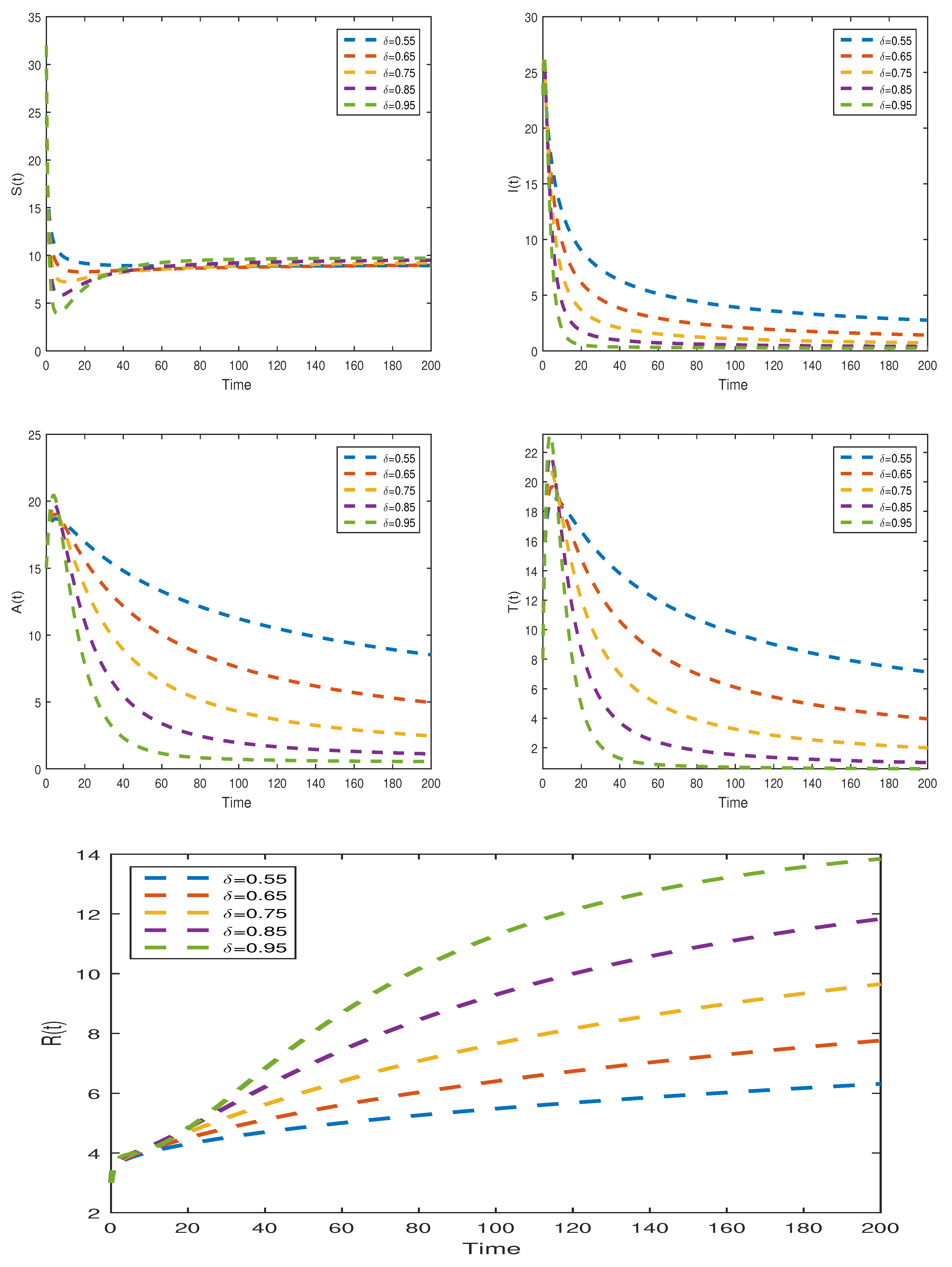
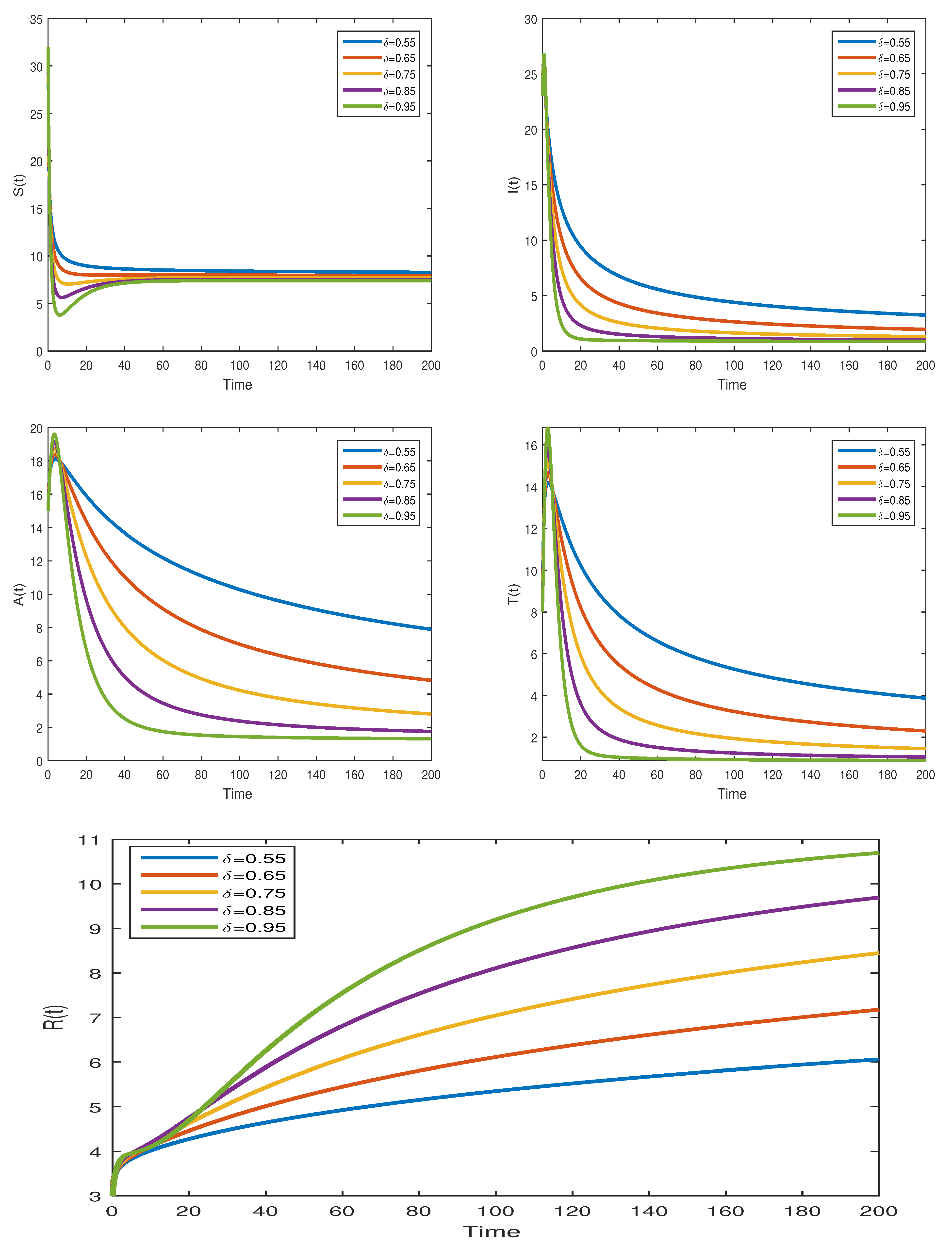
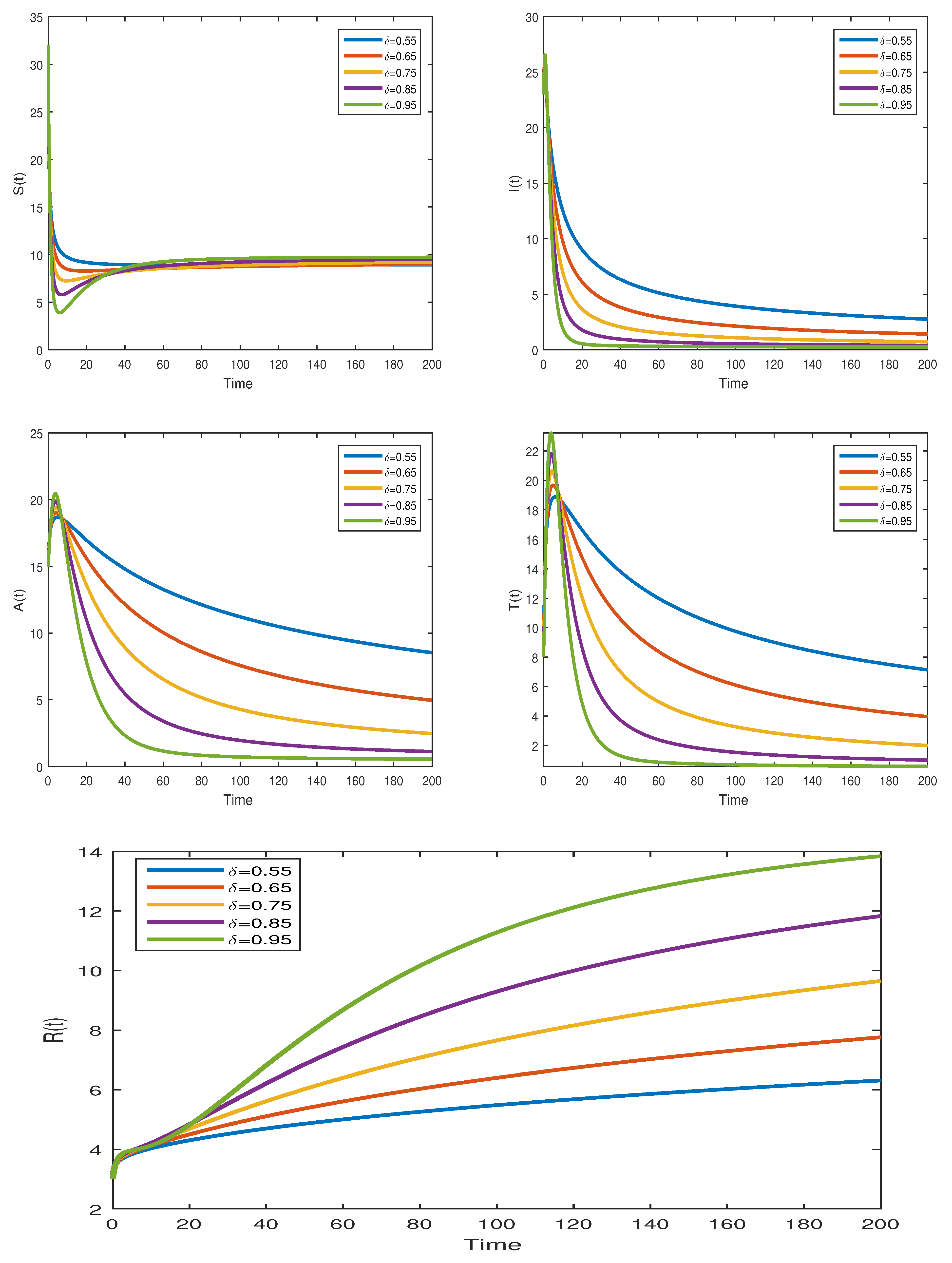
7.2.4. Graphical Results Model (31)

This part of the paper uses graphical results to demonstrate the behavior of the disease anticipated by model (1). The major purpose is to investigate how the memory index and other crucial characteristics impact the patterns of the current HIV/AIDS pandemic and, eventually, the potential of regulating it. Besides the analytical results, we obtained an approximate solution of both ODE and fractional-order models by using the RK4 algorithm and Newton’s polynomials. The majority of the parameters’ values utilized in the simulations were taken from Table 1. Figure 4, Figure 5, Figure 6 and Figure 7 depict the influence of the order of the fractional derivatives by altering the values of $\delta$ (i.e., memory index). As illustrated in Figure 4a, the sensitive population declines for a time before dropping to a specific positive population irrespective of $\delta$. Similarly, Figure 4b explains the dynamics of the infectious individuals for choosing a suitable value of $\delta$ in a given range. The maxima of the infectious trajectories appeared relatively slower and marginally fewer for the lowest values of $\delta$. We repeated a similar process, and Figure 4c shows the dynamics of individuals with full-blown AIDS who are not taking ARV medication. Figure 4d depicts the dynamic of representing the number of people being treated as $\delta$ changes. Similarly, the dynamical behaviors of the people who have changed their lifestyle is illustrated in Figure 4e for different values of $\delta$. The behavior of the curves suggests that the recovered population rises initially and then asymptotically reaches the underlying equilibrium point.

8. Conclusions

In conclusion, we present an epidemic model to understand and combat HIV/AIDS infection utilizing the tools of ODE and fractional calculus by using the Caputo operator. The use of fractional calculus in modeling infectious diseases, such as HIV/AIDS, allows for a more accurate representation of the complex dynamics involved in the spread and control of the infection. The results of this work provide important insights into the role of both the Caputo fractional derivative and treatment strategies in controlling the spread of HIV/AIDS. The model’s global stability analysis also sheds light on the importance of early detection and treatment in reducing the impact of the disease on individuals and communities. As such, this study serves as a valuable resource for researchers and policymakers working towards mitigating the HIV/AIDS epidemic and improving public health outcomes. In this paper, we present an epidemic model that governs the transmission behavior of HIV/AIDS by incorporating the treatment class T. The equilibria of the model are investigated, and subsequently, the threshold quantity $R_0$ is calculated to describe the global dynamics of the model. It is proved that for $R_0<1$, the infection-free state of the model is globally asymptotically stable. However, as we increase the threshold number beyond one, the endemic equilibrium becomes globally asymptotically stable, and in such a case, the disease-free state is noted to be unstable. At the end of the paper, the obtained analytic conclusions regarding the ODE model are verified through numerical simulations. We also explore a fractional-order HIV/AIDS epidemic model, utilizing the Caputo fractional differential operator for dynamical behaviors. The model is investigated qualitatively, and computational modeling is used to examine the system’s long-term behavior. The existence and uniqueness of the solution to the proposed model are determined by applying some results from the fixed point theory. The stability analysis for the system is investigated by employing the Ulam–Hyers method. For numerical simulations, we use Newton’s polynomial and the Toufik–Atangana numerical method. The results of the paper demonstrate that the fractional-order approach in capturing the dynamics of the HIV/AIDS epidemic is effective, and it provides valuable insights for designing optimal control policies. Further, the findings of the study reveal that early medication for HIV/AIDS is crucial and can save money and lives alike.

References

1. Palella, F.J.; Delaney, K.M. Declining morbidity and mortality among patients with advanced human immunodeficiency virus infection. N. Engl. J. Med. 1998, 339, 405–406. [Google Scholar] [CrossRef] [PubMed]
2. Kandwal, R.; Garg, P.K.; Garg, R.D. Health GIS and HIV/AIDS studies; perspective and retrospective. J. Biomed. Inf. 2009, 42, 748–755. [Google Scholar] [CrossRef] [PubMed]
3. Lou, J.; Lou, Y.; Wu, J. Threshold virus dynamics with impulsive antiretroviral drug effects. J. Math. Biol. 2012, 65, 623–652. [Google Scholar] [CrossRef] [PubMed]
4. Chibaya, S.; Kgosimore, M. Mathematical analysis of drug resistance in vertical transmission of HIV/AIDS. Open J. Epidemiol. 2013, 3, 139–148. [Google Scholar] [CrossRef]
5. Naresh, R.; Tripathi, A.; Omar, S. Modelling the spread of AIDS epidemic with vertical transmission. Appl. Math. Comput. 2006, 178, 262–272. [Google Scholar] [CrossRef]
6. Waziri, A.S.; Makinde, O.D. Mathematical modelling of HIV/AIDS dynamics with treatment and vertical transmission. J. Appl. Math. 2012, 2, 77–89. [Google Scholar] [CrossRef]
7. Naresh, R.; Sharma, D. An HIV/AIDS model with vertical transmission and time delay. World J. Model. Simul. 2011, 7, 230–240. [Google Scholar]
8. Walensky, R.P.; Paltiel, A.D. The survival benefits of AIDS treatment in the united states. Infect. Dis. Soc. Am. 2006, 194, 11–19. [Google Scholar] [CrossRef]
9. Yusuf, T.; Benyah, F. Optimal strategy for controlling the spread of HIV/AIDS disease: A case study of South Africa. J. Biol. Dyn. 2012, 6, 475–494. [Google Scholar] [CrossRef]
10. Huo, H.F.; Feng, L.X. Global stability for an HIV/AIDS epidemic model with different latent stages and treatment. Appl. Math. Model. 2012, 37, 1480–1489. [Google Scholar] [CrossRef]
11. Meng, X.; Chen, L.; Cheng, H. Two profitless delays for the SEIRS epidemic disease model with nonlinear incidence and pulse vaccination. Appl. Math. Comput. 2007, 186, 516–529. [Google Scholar] [CrossRef]
12. Hsieh, Y.H.; Chen, C.H. Modelling the social dynamics of a sex industry: Its implications for spread of HIV/AIDS. Bull. Math. Biol. 2004, 66, 143. [Google Scholar] [CrossRef] [PubMed]
13. Diallo, O.; Kone, Y.; Pousin, J. A model of spatial spread of an infection with applications to HIV/AIDS in mali. Appl. Math. 2012, 3, 1877–1881. [Google Scholar] [CrossRef]
14. Sharomi, O.; Podder, C.N. Modelling the transmission dynamics and control of the novel 2009 swine influenza (h1n1) pandemic. Bull. Math. Biol. 2011, 73, 515–548. [Google Scholar] [CrossRef]
15. Taneco-Hernández, M.A.; Vargas-De-León, C. Stability and Lyapunov functions for systems with Atangana–Baleanu Caputo derivative: An HIV/AIDS epidemic model. Chaos Solitons Fractals 2020, 132, 109586. [Google Scholar] [CrossRef]
16. Ali, Z.; Rabiei, F.; Shah, K.; Khodadadi, T. Fractal-fractional order dynamical behavior of an HIV/AIDS epidemic mathematical model. Eur. Phys. J. Plus 2021, 136, 36. [Google Scholar] [CrossRef]
17. Jan, A.; Srivastava, H.M.; Khan, A.; Mohammed, P.O.; Jan, R.; Hamed, Y.S. In Vivo HIV Dynamics, Modeling the Interaction of HIV and Immune System via Non-Integer Derivatives. Fractal Fract. 2023, 7, 361. [Google Scholar] [CrossRef]
18. Almoneef, A.A.; Barakat, M.A.; Hyder, A.A. Analysis of the Fractional HIV Model under Proportional Hadamard-Caputo Operators. Fractal Fract. 2023, 7, 220. [Google Scholar] [CrossRef]
19. Algahtani, O.J.J. Comparing the Atangana-Baleanu and Caputo-Fabrizio derivative with fractional order: Allen Cahn model. Chaos Solitons Fractals 2016, 89, 552–559. [Google Scholar] [CrossRef]
20. Atangana, A.; Baleanu, D. New fractional derivatives with nonlocal and non-singular kernel: Theory and application to heat transfer model. Therm. Sci. 2016, 20, 763–769. [Google Scholar] [CrossRef]
21. Hilfer, R. Mathematical and physical interpretations of fractional derivatives and integrals. Handb. Fract. Calc. Appl. 2019, 1, 47–85. [Google Scholar]
22. van den Driessche, P. Reproduction numbers and sub-threshold endemic equilibria for compartmental models of disease transmission. Math. Biosci. 2002, 180, 29–48. [Google Scholar] [CrossRef] [PubMed]
23. Gautam, R. Reproduction numbers for infections with free-living pathogens growing in the environment. J. Biol. Dyn. 2012, 6, 923–940. [Google Scholar]
24. Cheng, Y.; Wang, J.; Yang, X. On the global stability of a generalized cholera epidemiological model. J. Biol. Dyn. 2012, 6, 1088–1104. [Google Scholar] [CrossRef] [PubMed]
25. Li, G.H.; Jin, Z. Global stability of a SEIR epidemic model with infectious force in latent, infected and immune period. Chaos Solitons Fractals 2005, 25, 1177–1184. [Google Scholar] [CrossRef]
26. LaSalle, J.P. The stability of dynamical systems. In Regional Conference Series in Applied Mathmatics; Society for Industrial and Applied Mathematics: Philadelphia, PA, USA, 1976; Volume 25. [Google Scholar]
27. Huo, H.F.; Feng, L.X. Global stability of an epidemic model with incomplete treatment and vaccination. Discret. Dyn. Nat. Soc. 2012, 14, 530267. [Google Scholar] [CrossRef]
28. Naresh, R.; Tripathi, A.; Sharma, D. Modelling and analysis of the spread of AIDS epidemic with immigration of HIV infectives. Math. Comput. Model. 2009, 49, 880–892. [Google Scholar] [CrossRef]
29. Yang, X.; Wu, L.; Zhang, H. A space-time spectral order sinc-collocation method for the fourth-order nonlocal heat model arising in viscoelasticity. Appl. Math. Comput. 2023, 2023457, 128192. [Google Scholar] [CrossRef]
30. Jiang, X.; Wang, J.; Wang, W.; Zhang, H. A Predictor–Corrector Compact Difference Scheme for a Nonlinear Fractional Differential Equation. Fractal Fract. 2023, 7, 521. [Google Scholar] [CrossRef]
31. Zhang, H.; Han, X. Quasi-wavelet method for time-dependent fractional partial differential equation. Int. J. Comput. Math. 2013, 90, 2491–2507. [Google Scholar] [CrossRef]
32. Atangana, A.; Araz, S.I. New Numerical Scheme with Newton Polynomial: Theory, Methods, and Applications; Academic Press: New York, NY, USA, 2021. [Google Scholar]
33. Atangana, A.; İğret Araz, S. Mathematical model of COVID-19 spread in Turkey and South Africa: Theory, methods, and applications. Adv. Differ. Equ. 2020, 2020, 659. [Google Scholar] [CrossRef]
34. Zarin, R.; Khan, A.; Kumar, P. Fractional-order dynamics of Chagas-HIV epidemic model with different fractional operators. AIMS Math. 2022, 7, 18897–18924. [Google Scholar] [CrossRef]
35. İğret Araz, S. Analysis of a Covid-19 model: Optimal control, stability and simulations. Alex. Eng. J. 2021, 60, 647–658. [Google Scholar] [CrossRef]
36. Kumar, S.; Kumar, A.; Jleli, M. A numerical analysis for fractional model of the spread of pests in tea plants. Numer. Methods Partial. Differ. Equ. 2022, 38, 540–565. [Google Scholar] [CrossRef]
37. Kumar, S.; Kumar, A.; Samet, B.; Dutta, H. A study on fractional host–parasitoid population dynamical model to describe insect species. Numer. Methods Partial. Differ. Equ. 2021, 37, 1673–1692. [Google Scholar] [CrossRef]
Figure 1. The plots examine how changes in various parameters relate to R 0 through sensitivity analysis. (a) R 0 versus sensitive parameters k 2 and β ; (b) R 0 versus sensitive parameters d and α 1 ; (c) R 0 versus sensitive parameters α 2 and Λ ; (d) R 0 versus sensitive parameters δ 2 and d; (e) R 0 versus sensitive parameters δ 2 and α 2 ; (f) R 0 versus sensitive parameters μ 1 and k 1 .
Fractalfract 07 00643 g001
Figure 2. When R 0 = 0.89256 < 1 ,   α 1 = 0.08 ,   α 2 = 0.03 , the disease-free state E 0 is globally asymptotically stable.
Fractalfract 07 00643 g002
Figure 3. For R 0 = 1.24672 > 1 ,   α 1 = 0.25 ,   α 2 = 0.01 , the plot shows the global asymptotic stability of the endemic state E * .
Fractalfract 07 00643 g003
Figure 4. The behavior of each state variable of the Caputo fractional model via Newton’s polynomial numerical method for EE case is depicted in the figure.
Fractalfract 07 00643 g004
Figure 5. The behavior of each state variable of the Caputo fractional model via Newton’s polynomial numerical method for DFE case is depicted in the figure.
Fractalfract 07 00643 g005
Figure 6. The behavior of each state variable of the Caputo fractional model via Toufik–Atangana numerical method for DFE case is depicted in the figure.
Fractalfract 07 00643 g006
Figure 7. The behavior of each state variable of the Caputo fractional model via Toufik–Atangana numerical method for DFE case is depicted in the figure.
Fractalfract 07 00643 g007