Abstract
Recent years have seen an increase in scientific interest in the El Nio/La Nia Southern Oscillation (ENSO), a quasiperiodic climate phenomenon that takes place throughout the tropical Pacific Ocean over five years and causes significant harm. It is associated with the warm oceanic stage known as El Nio and the cold oceanic stage known as La Nia. In this research, the ENSO model is considered under a fractional operator, which is defined via a nonsingular and nonlocal kernel. Some theoretical features, such as equilibrium points and their stability, bifurcation maps, the existence of a unique solution via the Picard–Lindelof approach, and the stability of the solution via the Ulam–Hyres stability approach, are deliberated for the proposed ENSO model. The Adams–Bashforth numerical method, associated with Lagrangian interpolation, is used to obtain a numerical solution for the considered ENSO model. The complex dynamics of the ENSO model are displayed for a few fractional orders via MATLAB-18.
1. Introduction
A mathematical model is an easy and cheap tool with whcih to investigate problems in ocean and atmospheric engineering [1,2,3]. Our interest is in the analysis of climate changes produced via the ocean and the atmosphere. The ENSO phenomenon, which has been the subject of many studies, dominates the decadal climatic changes that result from the interplay of the tropical ocean and the atmosphere. Over the past ten years, the idea of the ENSO phenomenon has grown to a more developed stage. ENSO research has developed to the point where forecasts are now routinely made. In its investigation of the empirical relationships between El Nio and the Southern Oscillation, Ref. [4] originally proposed that ENSO is the outcome of ocean–atmosphere interaction in the tropical Pacific. He understood that the easterlies across the tropical Pacific are caused by the equatorial SST zonal gradient. By producing a cold SST over the eastern Pacific, these easterlies, in turn, enhance the SST gradient. A hot or cold SST anomaly is maintained through the Bjerknes positive feedback process of tropical ocean–atmosphere interaction. Wyrtki, in [5], discovered that oceanic anomalies in sea-level data are dynamic and basin-wide during an El Nio. He proposed that the strengthening of the trade winds is related to the rise in sea level, which is a measure of the heat content over the western Pacific. The stored warm water then moves eastward in the form of Kelvin waves to initiate an El Nio event.
La Nia has low air surface pressure and El Nio has high air surface pressure in the tropical western Pacific. The eastern equatorial Pacific Sea surface temperature u (t) and the thermocline depth anomaly v (t) are provided by the perturbation coefficient in the dynamics of recounting the oscillating physical mechanism of the ENSO model, as shown in [6,7] and the following:
where , and are physical constants. System (1) has many physical applications in ocean engineering and is analyzed from a different of point of view. Studying ENSO holds great significance for several compelling reasons. First, ENSO is a natural climate pattern with far-reaching impacts on weather and climate conditions worldwide. This understanding is invaluable for meteorologists, climatologists, and policymakers as it allows them to anticipate and prepare for extreme weather events, including droughts, floods, and hurricanes, often associated with El Niño and La Niña phases.
Moreover, ENSO’s influence extends beyond meteorology, profoundly affecting ecosystems, agriculture, fisheries, and water resources in diverse regions across the globe. By grasping the intricacies of ENSO and its oscillations, scientists and decision-makers can develop more effective strategies for managing water resources, planning agricultural practices, and conserving biodiversity, enhancing overall resilience to environmental changes.
Additionally, the interactions between ENSO and other climate patterns, such as the Indian Ocean Dipole and the Pacific Decadal Oscillation, underscore the interconnected nature of global climate systems. This awareness plays a crucial role in refining climate models and making more accurate long-term climate predictions, essential for adapting to and mitigating the effects of climate change, ultimately shaping a more sustainable future for our planet.
Fractional calculus (FC) is a hot research topic nowadays due to its interesting properties and applications [8,9,10,11]. In the literature, several operators have been introduced for the analysis of mathematical models that occur in various disciplines. Three main operators, i.e., Caputo, Caputo–Fabrizio (CF) and Atangana–Baleanu (AB) operators, are very popular and have been frequently used in the investigation of physical phenomena [12,13,14]. These operators are dependent on the distinct nature of kernels. Amongst these, the operator defined via the Mittag–Leffler kernel, which we call the Atangana–Baleanu (AB) operator, gives better results than the others. The AB operator has many applications in different fields of applied sciences such as mathematical physics [15,16,17], biomathematics [18,19], chaotic systems [20], and many more [21,22].
The relevance of using a fractional operator in the ENSO model lies in its ability to capture complex and long-range interactions within the system. ENSO is a highly intricate climate phenomenon influenced by a wide range of factors operating across different spatial and temporal scales. By employing a fractional operator, the model can effectively account for nonlocal interactions and memory effects that play a significant role in ENSO dynamics. This approach allows for a more accurate representation of the system’s behavior, leading to a better understanding of ENSO’s complexities and improved predictions of its behavior over time. Using the concept presented in [23], we can change the fractional operator with an auxiliary parameter , having the dimension of sec. stands for, to make sure that the dimension is the same on both sides. Therefore, we can express the Equation (1) in the fractional sense of correct dimensions as follows:
subject to initial values (IV) and . In the system (2), denotes the fractional AB differential operator which is defined below. Let FD denote the fractional derivative.
Definition 1
([24]). For fractional order , and , the FD is defined as follows:
where signifies the normalization function, , and represents Mittag–Leffler function in one parameter as given below:
Let FI represent fractional integral. The corresponding inverse operator of the is defined as follows.
Definition 2
([24]). For fractional order and , x FI is defined as follows:
2. Equilibria and Bifurcation
Here, we study the equilibrium points (EPs) and the stability of the considered mode. For the EPs, we equate the left side of model (2) to zero, so we have
On solving Equation (3), for and , we obtain
The Jacobian matrix of the considered model is as follows:
Putting the values of parameters in Equation (2), we obtain complex complex equilibrium points, which we do not consider. We consider the first equilibrium point ; therefore, after putting the first equilibrium point in Equation (5), we obtain the eigen values as and , which shows that the proposed system is a stable spiral with damped oscillatory behavior.
Bifurcation
Here, we graphically present the bifurcation in the proposed model (2) vs. different parameters.
Figure 1 conveys the bifurcation in the state variable of model (2) vs. parameter . Figure 2 gives the bifurcation in the state variable of model (2) vs. parameter . Figure 3 displays the bifurcation in the state variable of model (2) vs. parameter . In Figure 1, we observe the period doubling bifurcation. Figure 2 and Figure 3 depict the inverse period doubling bifurcations.

Figure 1.
The bifurcation in of model (2) vs. .
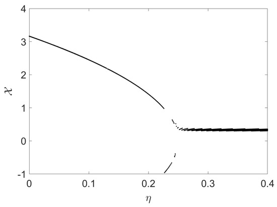
Figure 2.
The bifurcation in of model (2) vs. .
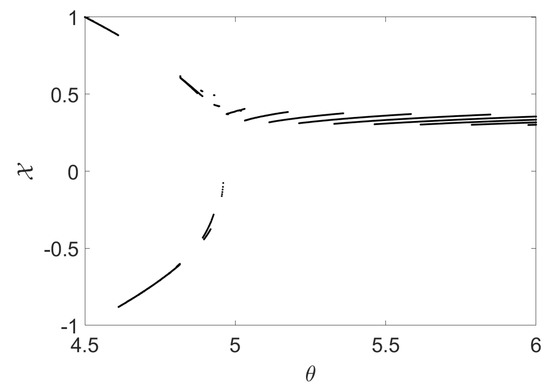
Figure 3.
The bifurcation in of model (2) vs. .
3. Some Theoritical Results
The theoretical and qualitative analysis of differential equations under FDs has gained much interest among scientists. Several approaches have been implemented to study these theoretical characteristics. In this section, some famous fixed point results are utilized to demonstrate some qualitative features such as the existence and stability of the solution of the ENSO model under the AB fractional operator. Let us write the ENSO model under AB as follows:
Here, we utilize the Picard–Lindelof approach and fixed-point theory to show that the ENSO model has a solution. One may write model (6) in an alternative form as follows:
where and denote the right hand sides of Equation (6). From here on, consider .
Theorem 1.
If and , then the kernels and fulfill the Lipschitz condition.
Proof.
Let , and where , , and . In the start, we demonstrate that the contraction requirement is met by . For this, consider
Thus, satisfies the contraction condition by taking . Now, consider the second equation as follows:
Thus, satisfies the contraction condition by taking □
One way to express the system (7) is as follows:
Here, we obtain the subsequent iterative equations
Now, we achieve the exact solution by taking the limit .
Theorem 2.
The considered system posses a unique solution if
Proof.
Let , where
Define the Picard operator as follows:
where
and
Since and satisfies the contraction condition,
Additionally, we assume that the solution is bounded, i.e.,
Thus, we need As a consequence, using Banach contraction result, one obtains
Now we have
where . Since ℜ fulfills the criteria of contraction, the suggested ENSO model has a unique solution. □
4. Numerical Results
Model (2) ’s approximative solutions are provided in this section. A numerical technique is developed using the fractional Adams–Bashforth approach to simulate our system. The recommended scheme allows for the capture of numerical simulations. To obtain numerical results, consider
where , and Using integral, we have
Now, to deduce the numerical results, set , for , then
The function is approximated in the via Lagrangian interpolation as
Sos system (13) obtains the form:
Now,
At , we obtain
Likewise,
So, system (14) becomes
Similarly,
5. Stability Analysis
Here, we exhibit the stability of the solution of the coupled ocean model under operator using the concept of Ulam–Hyres () stability. We present the following definitions which will be used in the stability solution. Let us write the proposed ENSO model as
where
Next, we apply the integral operator in the ABC sense on (15)
Next, we define operator by
Definition 3
Definition 4
([25]). The solution of AB ENSO model (2) is stable if with for each solution which satisfies
with , and , for i = 1, 2.
Definition 5
Definition 6
([25]). The ENSO system (2) is stable with respect to if ∃; thus, for each solution of
we have , so
with and for i = 1, 2.
Remark 1.
satisfies (19) ⇔ there is (depending on ), so
- ;
- .
Remark 2.
is the solution of (21) ⇔ there is (depending on ), so
- ;
- .
Remark 3.
Consider an increasing mapping and let , so ∀. Here, we obtain
Stability
Here, we ellaborate the important result which factor into the and stability of the proposed model (2).
Lemma 1.
Suppose that and is the solution of (19). Then, satisfies the following:
Proof.
Consider that is the solution of (19). Then, we have
The solution of the above equation can expressed as
Using Remark 3, we obtain
Hence, we obtained the inequality (27). □
Next, we demonstrate the and stability of the solutions to the proposed model (2).
Theorem 3.
Suppose that and satisfies the Lipchitz condition. Then, model (2) is stable on .
Proof.
Consider that is any solution of (19) and is a unique solution of model (2). Using triangle inequality with Lemma (1), we obtain
which shows that , where
So, the suggested model (2) is stable. □
Corollary 1.
Considering in the above theorem with , model (2) is stable.
Lemma 2.
Suppose that and is the solution of (21). Then, satisfies the following:
Proof.
Consider that is the solution of (21). Then, one reaches:
The solution of the above equation can expressed as
Using Remark 4, we obtain
Hence, we obtained the inequality (33). □
Next, we prove that the suggested model (2) is and stable.
Theorem 4.
Suppose that and satisfies the Lipchitz condition . Then, model (2) is stable on
Proof.
Consider that is any solution of (24) and is a unique solution of model (2). Using triangle inequality with Lemma (2), we obtain
which shows that , where
So, the suggested model (2) is stable. □
Corollary 2.
Considering in the above theorem with , model (2) is stable.
6. Numerical Simulations
Here, we numerically simulate the approximate results using various values of parameters and fractional orders. For the simulations of the outcomes, the initial conditions are considered as .
In Figure 4, the parameters values are considered as , . The fractional order is considered as , , , and . Figure 4a shows the 2D dynamics of the sea surface temperature and thermocline depth anomaly . Figure 4b depicts the 3D behavior of the state variables and vs. time t. Further, Figure 4c,d visualizes the evolution of the waves in the state variables and vs. t, respectively. In Figure 4, the damping behavior can be observed; further, it is observed that the fractional order operators decrease the wave amplitude, which shows the existence of a fixed point attractor that attracts all the nearby trajectories towards it.
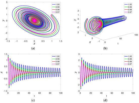
Figure 4.
The dynamics of model (2) with various fractional orders.
In Figure 5, different values of parameter are considered as , , , and . The fractional order is considered as . Decreasing the value of parameter reduces the number of oscillations in the proposed system. Figure 5a shows the 2D dynamics of the sea surface temperature and thermocline depth anomaly . Figure 5b,c visualize the evolution of the waves in the state variables vs. t, respectively.
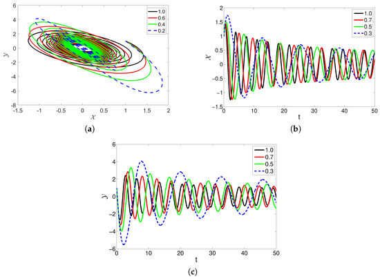
Figure 5.
The dynamics of model (2) with different values of .
In Figure 6, different values of parameter are considered as , , , and . The fractional order is considered as . From Figure 6, we see that the decrease in the value of increases the amplitude of the oscillations. Figure 6a shows the 2D dynamics of the sea surface temperature and thermocline depth anomaly . Figure 6b,c visualize the evolution of the waves in the state variables vs. t, respectively.
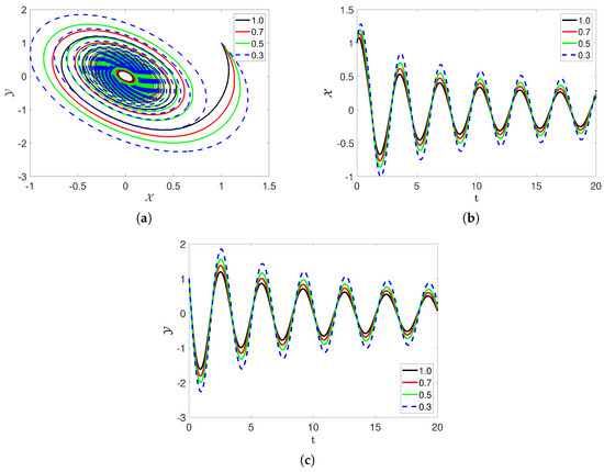
Figure 6.
The affects of different values of parameter on the dynamics of model (2).
In Figure 7, different values of parameter are considered as , , , and . Here, the fractional order is considered as . Figure 7a displays the 2D dynamics of vs. with . Figure 7b demonstrates the behavior of sea surface temperature vs. time t, along with thermocline depth anomaly vs. time t. The increase in the parameter decreases the oscillations. Figure 7c visualize the evolution of the waves in the state variable vs. t.
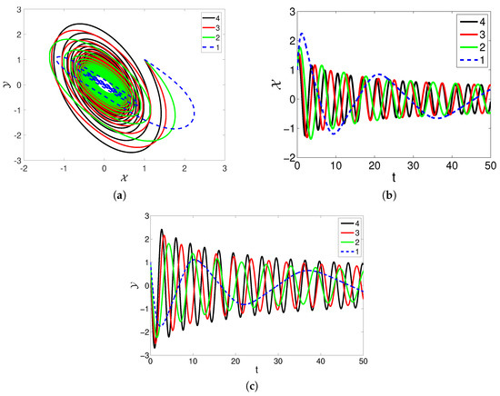
Figure 7.
The affects of different values of parameter on the dynamics of model (2).
In Figure 8, different values of parameter are considered as , , , and . For this figure, the fractional order is considered as . From the varying , one can observe that decreasing increases the number as well as amplitudes of the waves with the passage of time. Figure 8a shows the 2D dynamics of the sea surface temperature and thermocline depth anomaly . Figure 8b,c visualize the evolution of the waves in the state variables vs. t, respectively.
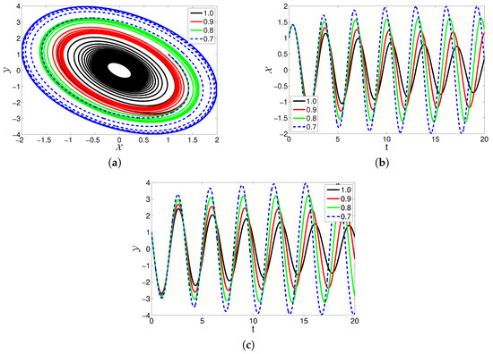
Figure 8.
The affects of different values of parameter on the dynamics of model (2).
7. Conclusions
Young researchers have always been drawn to the study of the complicated nature of realistic models in order to share their ideas and highlight the innovative characteristics of the relevant system. In this article, we have used a coupled system, the ENSO model with a Mittag–Leffler fractional derivative, to represent the atmospheric ocean. We have exhibited results indicating the existence of, at most, one solution to the considered model by applying the Picard–Lindelof theory and the Banach contraction theorem. We have analyzed the equilibrium points and have presented their stability. We have depicted the different natures of bifurcation maps with respect to various parameters. We have used the two-step Adams–Bashforth method and Lagrangian interpolation polynomial to procure numerical results for the projected ENSO model. In parametric graphs, the ENSO model under consideration’s complexity has been depicted for various fractional orders. The figures illustrate the behavior of several parameters related to the coupled system after analysis. Additionally, the employed system has a significant impact on how water and weather affect living things on a regular basis. Therefore, the current study helps researchers to learn more about the model and makes room for innovation.
Author Contributions
Methodology, Y.Z., P.L., C.X. and X.P.; Software, Y.Z., P.L. and R.Q.; Formal analysis, Y.Z., P.L., C.X., X.P. and R.Q.; Investigation, Y.Z., P.L., C.X. and R.Q.; Writing-original draft, Y.Z., P.L., C.X. and X.P.; Writing-review & editing, Y.Z., P.L., C.X., X.P. and R.Q. All authors have read and agreed to the published version of the manuscript.
Funding
This work is supported by Project of High-level Innovative Talents of Guizhou Province ([2016]5651).
Data Availability Statement
No data has been used to support this study.
Conflicts of Interest
The authors declare no conflict of interest.
References
- Varsoliwala, A.C.; Singh, T.R. Mathematical modeling of tsunami wave propagation at mid ocean and its amplification and run-up on shore. J. Ocean Eng. Sci. 2021, 6, 367–375. [Google Scholar] [CrossRef]
- Li, J.; Liao, S. On the dynamics of the gravitational lifting system in the deep sea mining industry. J. Ocean Eng. Sci. 2021, 6, 400–404. [Google Scholar] [CrossRef]
- Rajapriyadharshini, J.R. An improved smoothed particle hydrodynamics approach using new inverse kernel function. J. Ocean Eng. Sci. 2022, 7, 327–336. [Google Scholar] [CrossRef]
- Bjerknes, J. Atmospheric teleconnections from the equatorial. Pac. Mon. Weather Rev. 1969, 97, 163–172. [Google Scholar] [CrossRef]
- Wyrtki, K. El Niño, the dynamic response of the equatorial Pacific Ocean to atmospheric forcing. J. Phys. Oceanogr. 1975, 5, 572–584. [Google Scholar] [CrossRef]
- Zeng, Y. The Laplace-Adomian-Pade Technique for the ENSO Model. Math. Probl. Eng. 2013, 2013, 954857. [Google Scholar] [CrossRef][Green Version]
- Singh, J.; Kumar, D.; Nieto, J.J. Analysis of an El Nino-Southern Oscillation model with a new fractional derivative. Chaos Solitons Fractals 2017, 99, 109–115. [Google Scholar] [CrossRef]
- Ou, W.; Xu, C.; Cui, Q.; Liu, Z.; Pang, Y.; Farman, M.; Ahmad, S.; Zeb, A. Mathematical study on bifurcation dynamics and control mechanism of tri-neuron BAM neural networks including delay. Math. Methods Appl. Sci. 2023. [Google Scholar] [CrossRef]
- Xu, C.; Mu, D.; Pan, Y.; Aouiti, C.; Yao, L. Exploring bifurcation in a fractional-order predator-prey system with mixed delays. J. Appl. Anal. Comput. 2023, 13, 1119–1136. [Google Scholar] [CrossRef]
- Xu, C.; Mu, D.; Liu, Z.; Pang, Y.; Liao, M.; Li, P. Bifurcation dynamics and control mechanism of a fractional-order delayed Brusselator chemical reaction model. MATCH Commun. Math. Comput. Chem. 2023, 89, 73–106. [Google Scholar] [CrossRef]
- Xu, C.J.; Cui, X.H.; Li, P.L.; Yan, J.L.; Yao, L.Y. Exploration on dynamics in a discrete predator-prey competitive model involving time delays and feedback controls. J. Biol. Dyn. 2023, 17, 2220349. [Google Scholar] [CrossRef] [PubMed]
- Jhangeer, A.; Faridi, W.A.; Asjad, M.I.; Inc, M. A comparative study about the propagation of water waves with fractional operators. J. Ocean Eng. Sci. 2022; in press. [Google Scholar] [CrossRef]
- Alqahtani, R.T.; Ahmad, S.; Akgül, A. Dynamical analysis of bio-ethanol production model under generalized nonlocal operator in Caputo sense. Mathematics 2021, 9, 2370. [Google Scholar] [CrossRef]
- Ahmad, S.; Ullah, A.; Partohaghighi, M.; Saifullah, S.; Akgül, A.; Jarad, F. Oscillatory and complex behaviour of Caputo-Fabrizio fractional order HIV-1 infection model. AIMS Math. 2021, 7, 4778–4792. [Google Scholar] [CrossRef]
- Gulalai; Rihan, F.A.; Ahmad, S.; Rihan, F.A.; Ullah, A.; Al-Mdallal, Q.M.; Akgül, A. Nonlinear analysis of a nonlinear modified KdV equation under Atangana Baleanu Caputo derivative. AIMS Math. 2022, 7, 7847–7865. [Google Scholar] [CrossRef]
- Khan, A.; Ali, A.; Ahmad, S.; Saifullah, S.; Nonlaopon, K.; Akgül, A. Nonlinear Schrödinger equation under non-singular fractional operators: A computational study. Results Phys. 2022, 43, 106062. [Google Scholar] [CrossRef]
- Ali, A.; Khan, A.U.; Algahtani, O.; Saifullah, S. Semi-analytical and numerical computation of fractal-fractional sine-Gordon equation with non-singular kernels. AIMS Math. 2022, 7, 14975–14990. [Google Scholar] [CrossRef]
- Saifullah, S.; Ahmad, S.; Jarad, F. Study on the dynamics of a piecewise tumor–immune interaction model. Fractals 2022, 30, 2240233. [Google Scholar] [CrossRef]
- Naowarat, S.; Ahmad, S.; Saifullah, S.; de la Sen, M.; Akgül, A. Crossover dynamics of Rotavirus disease under fractional piecewise derivative with vaccination effects: Simulations with real data from Thailand, West Africa, and the US. Symmetry 2022, 14, 2641. [Google Scholar] [CrossRef]
- Gao, F.; Li, W.Q.; Tong, H.Q.; Li, X.L. Chaotic analysis of Atangana–Baleanu derivative fractional order Willis aneurysm system. Chin. Phys. B 2019, 28, 090501. [Google Scholar] [CrossRef]
- Xu, C.; Liu, Z.; Liao, M.; Yao, L. Theoretical analysis and computer simulations of a fractional order bank data model incorporating two unequal time delays. Expert Syst. Appl. 2022, 199, 116859. [Google Scholar] [CrossRef]
- Xu, C.; Liu, Z.; Yao, L.; Aouiti, C. Further exploration on bifurcation of fractional-order six-neuron bi-directional associative memory neural networks with multi-delays. Appl. Math. Comput. 2021, 410, 126458. [Google Scholar] [CrossRef]
- Gómez-Aguilar, J.F.; Rosales-García, J.J.; Bernal-Alvarado, J.J.; Córdova-Fraga, T.; Guzmán-Cabrera, R. Fractional mechanical oscillators. Rev. Mex. Fís. 2012, 58, 348–352. [Google Scholar]
- Atangana, A.; Baleanu, D. New fractional derivatives with nonlocal and non-singular kernel: Theory and application to heat transfer model. Therm. Sci. 2016, 20, 763–769. [Google Scholar] [CrossRef]
- Rus, I.A. Ulam stabilities of ordinary differential equations in a Banach space. Carpath. J. Math. 2010, 26, 103–107. [Google Scholar]
Disclaimer/Publisher’s Note: The statements, opinions and data contained in all publications are solely those of the individual author(s) and contributor(s) and not of MDPI and/or the editor(s). MDPI and/or the editor(s) disclaim responsibility for any injury to people or property resulting from any ideas, methods, instructions or products referred to in the content. |
© 2023 by the authors. Licensee MDPI, Basel, Switzerland. This article is an open access article distributed under the terms and conditions of the Creative Commons Attribution (CC BY) license (https://creativecommons.org/licenses/by/4.0/).