Article

Overcoming Nonlinear Dynamics in Diabetic Retinopathy Classification: A Robust AI-Based Model with Chaotic Swarm Intelligence Optimization and Recurrent Long Short-Term Memory

by
Yusuf Bahri Özçelik
and
Aytaç Altan
*
Department of Electrical Electronics Engineering, Zonguldak Bülent Ecevit University, Zonguldak 67100, Turkey
*
Author to whom correspondence should be addressed.
Fractal Fract. 2023, 7(8), 598; https://doi.org/10.3390/fractalfract7080598
Submission received: 30 June 2023 / Revised: 23 July 2023 / Accepted: 1 August 2023 / Published: 3 August 2023

Abstract

:
Diabetic retinopathy (DR), which is seen in approximately one-third of diabetes patients worldwide, leads to irreversible vision loss and even blindness if not diagnosed and treated in time. It is vital to limit the progression of DR disease in order to prevent the loss of vision in diabetic patients. It is therefore essential that DR disease is diagnosed at an early phase. Thanks to retinal screening at least twice a year, DR disease can be diagnosed in its early phases. However, due to the variations and complexity of DR, it is really difficult to determine the phase of DR disease in current clinical diagnoses. This paper presents a robust artificial intelligence (AI)-based model that can overcome nonlinear dynamics with low computational complexity and high classification accuracy using fundus images to determine the phase of DR disease. The proposed model consists of four stages, excluding the preprocessing stage. In the preprocessing stage, fractal analysis is performed to reveal the presence of chaos in the dataset consisting of 12,500 color fundus images. In the first stage, two-dimensional stationary wavelet transform (2D-SWT) is applied to the dataset consisting of color fundus images in order to prevent information loss in the images and to reveal their characteristic features. In the second stage, 96 features are extracted by applying statistical- and entropy-based feature functions to approximate, horizontal, vertical, and diagonal matrices of 2D-SWT. In the third stage, the features that keep the classifier performance high are selected by a chaotic-based wrapper approach consisting of the k-nearest neighbor (kNN) and chaotic particle swarm optimization algorithms (CPSO) to cope with both chaoticity and computational complexity in the fundus images. At the last stage, an AI-based classification model is created with the recurrent neural network-long short-term memory (RNN-LSTM) architecture by selecting the lowest number of feature sets that can keep the classification performance high. The performance of the DR disease classification model was tested on 2500 color fundus image data, which included five classes: no DR, mild non-proliferative DR (NPDR), moderate NPDR, severe NPDR, and proliferative DR (PDR). The robustness of the DR disease classification model was confirmed by the 10-fold cross-validation. In addition, the classification performance of the proposed model is compared with the support vector machine (SVM), which is one of the machine learning techniques. The results obtained show that the proposed model can overcome nonlinear dynamics in color fundus images with low computational complexity and is very effective and successful in precisely diagnosing all phases of DR disease.

1. Introduction

Diabetes is a lifelong metabolic disease that occurs when blood sugar rises in the body due to the pancreas’ inability to produce enough insulin hormone or to use insulin hormone effectively. Diabetes, which is among the top 10 causes of death in adults, is seen in 9.3% of adults aged 20–79 worldwide, according to 2019 data. This rate corresponds to 463 million adults. The number of adults aged 20–79 years living with diabetes has increased by 62% in the last 10 years, and it is predicted that 578 million adults will live with diabetes in 2030 globally [1].
Since diabetes brings with it many diabetes-related diseases, it causes serious negative effects on the quality of life of individuals. Diabetic retinopathy (DR), a specific microvascular complication of diabetes, is damage to the blood vessels in the retinal mesh layer due to diabetes [2]. The individual’s vision is impaired due to bleeding or fluid leaking from the blood vessels in the retinal mesh layer [3]. Since DR disease has a progressive process, patients are at risk of vision loss if the disease cannot be diagnosed at an early phase and the necessary treatment cannot be applied in a timely manner [4]. The incidence of DR disease in the community increases in parallel with the duration of diabetes and is generally seen in approximately 30% of diabetics [5]. The progression of DR disease needs to be limited in order to prevent diabetes patients from losing their vision. This can be possible by diagnosing DR disease at an early phase. Therefore, it is recommended that diabetic patients undergo retinal screening at least twice a year under the supervision of a specialist ophthalmologist [6]. However, these scans take a lot of time and require good experience and expertise. Detection and classification of DR disease in the current clinical diagnosis is mainly based on a specialist ophthalmologist’s in-depth examination of the color fundus image and then the assessment of the patient’s condition. This diagnostic method is a time-consuming and laborious process, which can lead to more errors. The high number of diabetic patients and the insufficient medical resources in some regions make this process even more difficult. Today, it has become inevitable to benefit from fast and reliable computerized automatic scanning and pre-diagnosis systems to overcome this problem and assist ophthalmologists [7,8]. In this study, a robust artificial intelligence (AI)-based hybrid classification model that can classify the phases of DR disease at an early phase with high accuracy and low computational complexity is proposed to make it possible to limit the progression of DR disease.
DR disease is essentially divided into two classes, non-proliferative DR (NPDR) and proliferative DR (PDR). NPDR is defined as the early phase of the disease, while PDR is defined as the advanced phase of the disease. The NPDR phase of the disease is separated into three classes as mild, moderate, and severe. In the mild NPDR phase of the disease, microaneurysms and a few small hemorrhages are seen in color fundus images. In the moderate NPDR phase of the disease, diffusely increased microaneurysms in at least one retinal layer, exudates, venous changes, hemorrhages, and intraretinal microvascular abnormalities are observed in color fundus images. In the severe NPDR phase of the disease, predominantly microaneurysms, exudates, hemorrhages, venous changes, diffuse arteriolar occlusions, and increases in intraretinal microvascular abnormality density are seen in color fundus images. In the PDR phase of the disease, in addition to the findings in the NPDR phase, retinal neovascularization and minimal fibrous tissue proliferation are detected in color fundus images [8,9,10,11]. These findings, shown in Figure 1, are distinctive features in diagnosing the disease and determining its phase. If these findings, which cause the patients’ vision to decrease and disappear, are diagnosed and treated immediately, the deteriorated process can be taken under control and delayed [6].
In recent years, digital-fundus-image-based scanning programs have been used to cope with DR disease. However, their use for larger populations is not common all over the world due to the cost factor [12]. Meanwhile, the rapid increase in diabetes patients makes the capabilities of current digital-fundus-image-based screening programs questionable because these programs are heavily dependent on manual grading, which takes a significant amount of time for each case [7]. Therefore, research in recent years has focused on the automatic detection of DR disease at an early phase so that patients do not experience vision loss. However, it is seen that nonlinear dynamics, especially chaoticity, in color fundus images are ignored in most studies. The motivation of this paper is to develop a robust model that can automatically diagnose and classify DR disease in fundus images by coping with nonlinear dynamics in the image. Color fundus images are classified according to the severity of DR disease by the classification model with low computational complexity, so that an end-to-end real-time classification can be obtained from the fundus image for the patient’s condition. The main contributions of this study are summarized as follows:
  • The presence of chaos in the images of each DR disease class along with the healthy class is revealed by fractal analysis.
  • Feature groups are extracted for each family by applying two-dimensional stationary wavelet transform (2D-SWT) with biorthogonal, reverse biorthogonal, Daubechies, Coiflet, symlet, and Fejer–Korovkin wavelet families to the dataset consisting of each DR disease class together with the healthy class.
  • The entropy- and statistical-based feature groups extracted for the 12 image matrices obtained as a result of three-level decomposition contain nonlinear dynamics representing the DR disease classes.
  • The features that keep the model performance high are selected with a wrapper approach consisting of the chaotic particle swarm optimization (CPSO) and k-nearest neighbor (kNN) algorithms in order to keep the computational complexity of the model at a minimum and to cope with the chaoticity in the fundus images.
  • The most suitable chaotic map, which improves the convergence speed and optimum solution of the optimization algorithm, is determined and included in the optimization process to obtain the highest classification accuracy with the least features.
  • The effect of the features selected by the chaotic wrapper approach on the model performance is examined for each wavelet family.
  • The selected optimum feature vectors are finally fed into the recurrent neural network-long short-term memory (RNN-LSTM) for classifying DR disease sub-types like PDR, mild NPDR, moderate NPDR, and severe NPDR.
  • The model with the best performance is proposed, which includes the three-level 2D-SWT technique based on the ‘bior 2.8’ wavelet family, the wrapper approach consisting of logistic-chaotic-map-based CPSO and kNN, and the RNN-LSTM network for DR disease classification.
  • It is shown by experimental results that the proposed model can cope with nonlinear dynamics, has low computational complexity, and can be used in real-time applications thanks to these features.
The rest of this paper is organized as follows. Section 2 presents the background of the study and related works on the diagnosis and classification of DR disease. The methodology that makes up the diagnosis and classification model for DR disease, including 2D-SWT with wavelet families, chaotic-based wrapper approach consisting of the kNN and CPSO algorithms, the RNN-LSTM classifier, and performance metrics, is described in Section 3. The results of this study and some concrete discussions proving the performance of the proposed model are provided in Section 4. Finally, Section 5 highlights the conclusions.

2. Background and Related Works

DR disease, which develops due to diabetes and occurs as a result of damage to the vessels in the retinal layer of the eye, can be treated and vision loss can be prevented when it is diagnosed effectively in the early phases. In the literature review, there are many AI-based studies for the diagnosis and classification of DR disease. In [13], an AI-based model consisting of four stages, namely preprocessing, feature extraction, feature reduction, and classification, was proposed for the early diagnosis of DR. In the preprocessing stage of the model, techniques such as image scaling, green channel subtraction, and top-bottom line transformation were used to improve fundus images. The optic disc and blood vessels were segmented by two independent U-Net models. The features of the fundus images were extracted by the convolutional neural network (CNN)-singular value decomposition (SVD) hybrid model. It was stated that 100 of the 256 extracted features were selected and used by SVD. In the classification layer of the model, transfer-learning-based Inception-v3 architecture is preferred. The highest performance of the proposed model in three different datasets was measured as 97.92%. In [14], a segmentation-based learning approach was proposed by utilizing deep learning to detect and classify DR and DR lesions. With the proposed approach, it is aimed to deal with irregular lesions of DR. Fundus images with different contrast, image resolution, and illumination were preprocessed, and image segments were removed from the preprocessed image. The image segments were fed into the CNN classifier considering the segment level to evaluate the DR probabilities. The performance of the proposed model was measured to be approximately 96.3%. In [15], the prognosis of microaneurysm and an early diagnosis system were introduced for an NPDR system that is capable of training effectively a deep CNN (DCNN) for the semantic segmentation of fundus images, which can improve the accuracy and efficiency of NPDR detection. In [16], a hybrid deep neural network (DNN) model based on feature extraction and optimization-based feature selection was proposed for the early detection of DR. The most important features in the dataset were extracted using principal component analysis (PCA). The firefly algorithm was applied to reduce the size of the feature matrix. The selected features were fed into the DNN to classify the DR dataset. The performance of the model was also compared with the predominant machine learning methods in terms of accuracy, recall, precision, specificity, and sensitivity, and it was reported that the results obtained were superior to the machine learning models of the proposed model.
It is noteworthy that in the detection and classification of many DR diseases today, swarm-based optimization algorithms are used either to improve the parameters of the proposed AI-based algorithms to overcome the hyperparameter problem or to select the features that maximize the classifier performance [17,18,19,20,21,22]. In [17], a model was proposed for the DR classification problem in which CNN parameters were optimized with a hybrid genetic and ant colony optimization (HGACO) algorithm. The proposed model was built in three stages. In the first step, the noise at the edges of the DR images was removed. In the second step, the region of interest (ROI) features were extracted from the DR images using K-means cluster-based growing region segmentation. In the final stage, DR images were classified at four severity levels with the HGACO-based CNN algorithm. It was reported that the accuracy performance of the proposed model was measured as 97.7%. In [21], the severity of DR was categorized using a two-level classification strategy. At the first level, DR in fundus images was detected using SqueezeNet tuned by hybridized fractional war strategy optimization. At the second level, DR disease was classified according to severity levels by DCNN trained with the designed fractional war royale optimization algorithm. It was stated that the accuracy performance of the proposed strategy was measured as 91.6% at the first level and 91.1% at the second level. In the literature, there is no study that addresses both the model hyperparameter problem and high classification accuracy in the classification of DR disease. This study presents a model with both low computational cost and high classification accuracy to classify DR disease by overcoming nonlinear dynamics in fundus images.

3. Framework of the Diagnosis and Classification Algorithm for Diabetic Retinopathy

This section introduces our approach framework that can classify DR disease with minimal model complexity and high accuracy. Entropy- and statistical-based feature groups in the fundus image set, which consists of each DR disease class together with the healthy class and includes nonlinear dynamics, are extracted by 2D-SWT using biorthogonal, reverse biorthogonal, Daubechies, Coiflet, symlet, and Fejer–Korovkin wavelet families. To cope with the chaoticity in the fundus images, feature selection is performed with a wrapper approach consisting of the CPSO and kNN algorithms. The fitness function of the optimization algorithm is formed to obtain the highest model performance with the least computational cost. The selected feature vectors are finally fed into the RNN-LSTM, and the DR disease classification performance of the model is tested. The methodology used in our DR classification model is presented in detail in the following subsections.

3.1. Stationary Wavelet Transform

Wavelet transform, which is mostly preferred in the analysis of non-stationary signals, is a transform technique that separates the data into different frequency components and examines each component with its resolution at that scale [23]. Wavelet transform uses scalable windows that can be shifted along the signal. In this way, spectral behavior can be examined for each new location. Wavelets that provide a good tool for time–frequency analysis are mathematical functions that decompose data into different frequency components and then express each component with a resolution matched to the scale of the component. The priority in the wavelet transform is to choose the prototype function called the parser or mother wavelet [24]. Time analysis is performed with a compressed high-frequency version of the mother wavelet. Similarly, this analysis is repeated with the extended low-frequency version of the mother wavelet. The original signal is expressed in terms of the coefficients of a propagating wavelet. If a wavelet that is well matched to the original signal is selected, or if coefficients below a certain threshold value are assigned, the most approximate partial representation of the original signal is obtained.
There are two types of wavelet transforms, the continuous wavelet transform ( C W T ) and the discrete wavelet transform ( D W T ). The C W T of signal x ( t ) is represented as
C W T ψ X a , b = x ( t ) , ψ a , b ( t ) = + x t ψ a , b * t d t
where * indicates the complex conjugate operation, ψ ( t ) is the mother wavelet, x ( t ) is a square integrable function, and ψ a , b ( t ) is the wavelet family and is expressed as
ψ a , b ( t ) = 1 a   ψ t b a
where a 0 and b are real and positive numbers representing scaling and shifting parameters, respectively. Note that the wavelet function is a function of two variables, scale and position coefficients, while the original function x ( t ) is only a function of time. The inverse C W T of a signal is possible if the mother wavelet function ψ ( t ) satisfies the admissibility criterion, which is given by
C ψ = + ψ ( s ) 2 s d s <
and requires that the Fourier transform ψ ( s ) of ψ ( t ) satisfies certain properties. The admissibility criterion ensures that ψ ( t ) has finite energy, is localized both in time and frequency domains, and has a zero mean. This allows for the wavelet transform to be applied to signals of finite energy. If 0 < C ψ < , then the inverse C W T is mathematically defined as [25]:
x t = C W T ψ X a , b 1 = 1 C ψ a = 0 + b = + 1 a 2 C W T ψ X a , b ψ a , b t d b d a
Thus, the function can be synthesized from its wavelet transform by integrating over all scales and shifts.
C W T is a powerful tool for analyzing non-stationary signals in continuous time, but it requires a lot of computations and memory resources. On the other hand, D W T operates on a discretized version of the signal, making it more efficient and practical for many applications. The D W T is a useful tool for signal processing and analysis, particularly in cases where efficiency, multiresolution analysis, discretization, and compression are important considerations [26,27]. The D W T of the signal can be represented as the inner product of the signal x ( t ) with a wavelet function ψ m , n that has been scaled and shifted using dyadic variables m and n , respectively. The D W T can also be expressed in terms of the original signal’s samples, x ( k ) , as
D W T ψ X m , n = x , ψ m , n = a 0 m / 2 k x ( k ) ψ m , n * k n a 0 m b 0 a 0 m
where ψ m , n * denotes the complex conjugate of the wavelet function, a 0 > 1 and b 0 > 0 are scaling and translation parameters, m and n are integers, and x ( t ) is the discrete signal being analyzed. The wavelet function ψ m , n is obtained from the mother wavelet function by scaling and shifting it using the parameters a 0 m and n a 0 m b 0 , respectively.
In the D W T , a signal is decomposed into a set of discrete frequency sub-bands by applying a series of low-pass and high-pass filters. However, the filter banks used in the D W T are not shift-invariant, which means that the D W T coefficients are not localized in time. The stationary wavelet transform (SWT) is a type of wavelet transform that aims to address the shift-variance problem of the D W T . The SWT is performed by convolving the signal with a series of shifted and scaled versions of a single wavelet function, similar to the D W T . However, unlike the D W T , the scaling factor is fixed at 1, which means that the wavelet function is not dilated or contracted as it moves across different scales. This results in a stationary property, which means that the wavelet coefficients at a given scale and position are not affected by the coefficients at neighboring scales and positions, which makes them more robust to noise and small signal variations [28].
The SWT is a variant of the D W T but with a different sampling scheme. While the scales in both transforms are dyadic, the SWT does not subsample time steps at each level, resulting in non-dyadic time sampling. The SWT can be considered as a representation that lies between the high-redundancy C W T and the non-redundant D W T in terms of redundancy. The SWT preserves a non-redundancy frequency representation by maintaining a dyadic sampling of the scales while having an almost continuous and uniform time sampling [29]. The general transformation equation of SWT can be written based on the coefficients c m , n calculated as follows:
c m , n = x , ψ m , n = k Z x ( k ) ψ m , n * ( k )
where ψ m , n * is the discrete wavelet defined by
ψ m , n * ( k ) = 2 m / 2 ψ 2 m k n
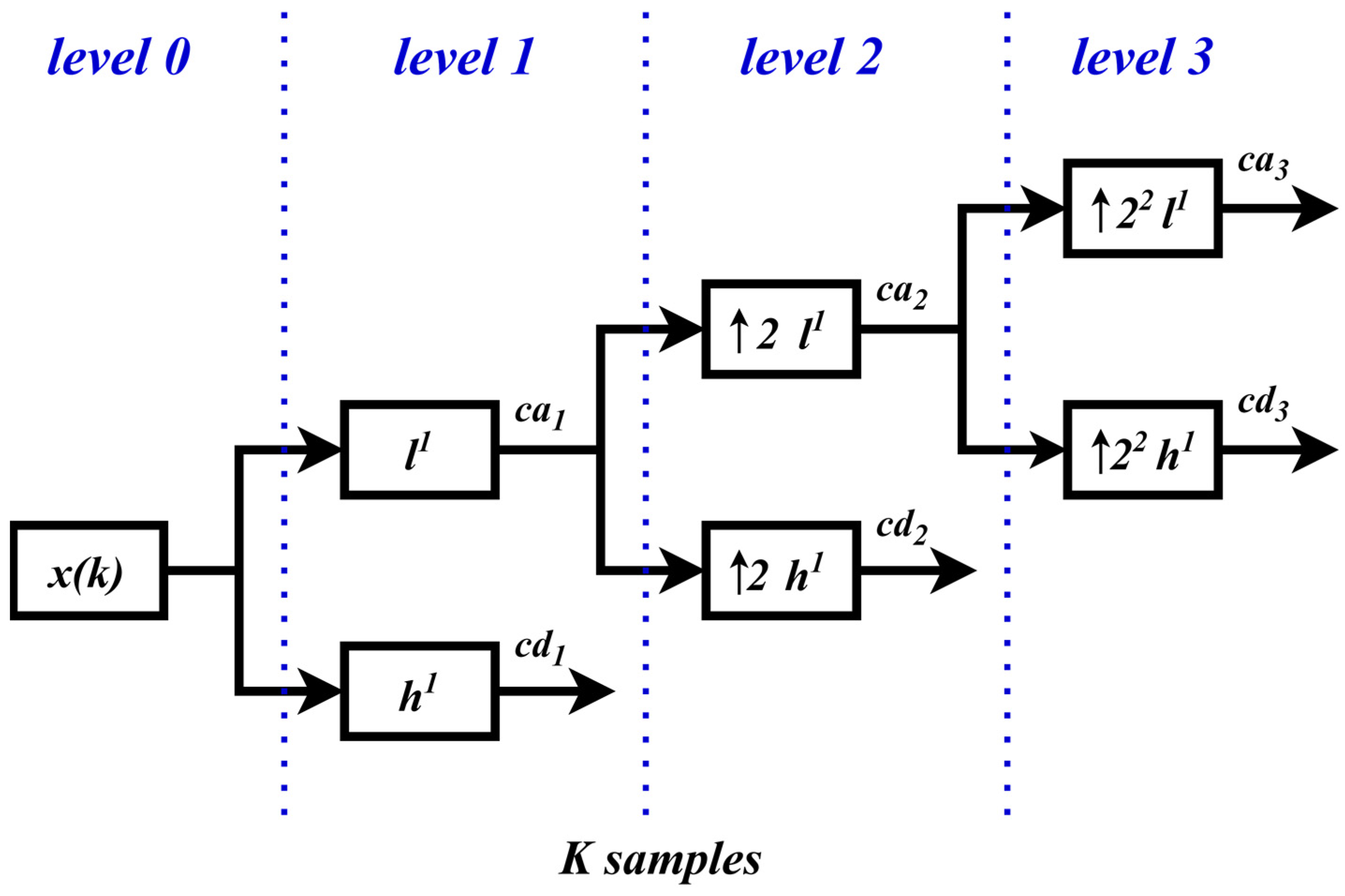
The scaling and wavelet coefficients, represented by c a m , n and c d m , n , respectively, are obtained through a convolution chain of the original signal sequence x ( k ) , along with the level-adaptive low-pass filter l 1 and high-pass filter h 1 . These filters are size-varying and adapt to the level of decomposition. The scaling coefficients provide an approximation of the signal, while the wavelet coefficients provide detailed information [30]. One can obtain the first scale and detail coefficients, c a 1 , n and c d 1 , n , of the SWT by convolving the input signal x ( k ) with the low-pass filter l 1 and high-pass filter h 1 , respectively. The calculation can be expressed as follows:
c a 1 , n ( k ) = k Z l 1 ( k τ ) x ( τ )
c d 1 , n ( k ) = k Z h 1 ( k τ ) x ( τ )
The above statement can be generalized to different coefficient scales by
c a m , n k = 2 m 1 l 1 * c a m 1 , n = k Z l m ( k τ ) c a m 1 , n ( τ )
c d m , n k = 2 m 1 h 1 * c a m 1 , n = k Z h m ( k τ ) c a m 1 , n ( τ )
where 2 m 1 l 1 = l m ( k ) is the oversampling of the low-pass filter l m 1 ( k ) coefficients, while 2 m 1 h 1 = h m ( k ) is the oversampling of the high-pass filter h m 1 ( k ) coefficients. These coefficients are expressed as
l m 2 k = l m 1 k
l m 2 k + 1 = 0
h m 2 k = h m 1 k
h m 2 k + 1 = 0
It is evident from Equations (10) and (11) that the low-pass filter l 1 and the high-pass filter h 1 are upsampled by a factor of two at each stage. As a result, the decomposition coefficients, namely approximation and detail, have the same length K C as the original signal x ( k ) , where K C = 2 m . This makes the output signal more accurate than the one obtained with D W T .
In our study, we used the SWT, which is capable of characterizing texture properties at multiple scales owing to its tight framework and fast iterative algorithm. The feature groups for each wavelet family were obtained using three-level SWT, as shown in Figure 2.

3.2. Multiresolution Analysis

It is possible to extract and classify features from signals in both the time domain and the frequency domain. Multiresolution analysis (MRA) based on the SWT is highly beneficial in extracting features from image signals. This approach can effectively separate undesirable components, such as trends and noise, from signals [31]. The computation of scaling and wavelet functions is utilized to analyze signals in both the time and frequency domains. The scaling function, denoted by φ m , n ( k ) , and the wavelet function, denoted by ψ m , n ( k ) , are defined by
φ m , n ( k ) = 2 m / 2 φ 2 m k n
ψ m , n ( k ) = 2 m / 2 ψ 2 m k n
where m , n Z . In SWT, the components with a high scale and low frequency correspond to the approximation coefficients φ ( k ) , whereas the components with a low scale and high frequency correspond to the detail coefficients ψ ( k ) . These coefficients are expressed by
φ ( k ) = k Z l ( k 2 n ) x ( k )
ψ ( k ) = k Z h ( k 2 n ) x ( k )
where l ( k ) and h ( k ) represent the coefficients of the low-pass filter and the high-pass filter, respectively.

3.3. Wavelet Families

The subsections following this one introduce the biorthogonal, Coiflet, Daubechies, Fejer–Korovkin, reverse biorthogonal, and symlet wavelet families that are utilized to compute the low- and high-pass filter coefficients of the SWT. Two-dimensional SWT (2D-SWT) with all the specified wavelet families was applied to the image set consisting of DR disease classes. The row and column of the image are, respectively, represented by the variables x and y . Horizontal, vertical, and diagonal directions correspond to ψ H , ψ V , and ψ D , respectively.

3.3.1. Biorthogonal Wavelet

Biorthogonal wavelets possess a compactly supported symmetrical structure that is not based on vanishing moments. In the biorthogonal scenario, there exist two scaling functions φ , φ ~ that can produce different MRA and correspondingly two distinct wavelet functions ψ , ψ ~ , instead of having only one scaling and wavelet function. The recursive computations of the scaling function and mother wavelet for orthogonal wavelets are denoted by [32]
φ ( k ) = 2 n l 0 ( n ) φ 2 k n
φ ~ ( k ) = 2 n l ~ 0 ( n ) φ ~ 2 k n
ψ ( k ) = 2 n h 1 ( n ) φ 2 k n
ψ ~ ( k ) = 2 n h ~ 1 ( n ) φ ~ 2 k n
where dual scaling functions φ ( k ) and φ ~ ( k ) , as well as dual mother wavelet functions ψ ( k ) and ψ ~ ( k ) , are related to a set of dual filter coefficients denoted by l 0 , l ~ 0 , h 1 , and h ~ 1 .
In this study, the 2D-SWT with the biorthogonal wavelet family was applied to the dataset consisting of DR disease classes. The scaling and wavelet functions of the ‘bior2.8’ wavelet, which provides the best classification performance for the biorthogonal wavelet family used in the study, are given in Figure 3.

3.3.2. Coiflet Wavelet

Coiflet wavelets are a family of wavelets introduced by Ingrid Daubechies. They are derived from scaling functions, are orthogonal and compactly supported, and have a high degree of smoothness, which make them useful in a variety of applications such as image compression, denoising, feature extraction, and analysis of signals containing sharp transitions or discontinuities [33]. The Coiflet wavelet of order N , denoted by ψ ( k ) , is defined as
ψ ( k ) = n = 0 2 N 1 l ( n ) φ 2 k n
where l ( n ) is the Coiflet scaling filter, and φ ( k ) is the scaling function. The scaling filter l ( n ) is obtained from the low-pass filter coefficients of the Daubechies wavelet of order 2 N 2 .
Coiflet wavelets are also characterized by their vanishing moments, which determine how well they can represent functions with different degrees of smoothness. The Coiflet wavelet of order N has 2 N 1 vanishing moments, which means it can accurately represent polynomials of a degree up to 2 N 2 . This property makes Coiflet wavelets particularly useful for analyzing signals that have a mixture of smooth and oscillatory behaviors [34].
In this study, the 2D-SWT with the Coiflet wavelet family was applied to the dataset consisting of DR disease classes. The scaling and wavelet functions of the ‘coif5’ wavelet, which provides the best classification performance for the Coiflet wavelet family used in the study, are given in Figure 4.

3.3.3. Daubechies Wavelet

The Daubechies wavelets are a family of orthonormal wavelets that are defined by a set of scaling coefficients and wavelet coefficients. They are characterized by their vanishing moments, which determine the degree of smoothness of the wavelet function. The Daubechies wavelets satisfy the admissibility condition, which guarantees that they form an orthonormal basis for L 2 ( R ) , the space of square-integrable functions over the real line. The filter coefficients for the Daubechies wavelets have finite support, meaning that they are non-zero only on a finite interval. The number of non-zero coefficients is 2 N 1 , where N is the order of the wavelet. The scaling function and wavelet function of the Daubechies of order N have a support size in the range of [ 0 , 2 N 1 ] , while the scaling function has 2 N non-zero scaling coefficients. This property makes them particularly useful for signal processing applications where a localized representation of the signal is important [35].
The scaling function φ ( k ) and the wavelet function ψ ( k ) of the Daubechies wavelets can be written as follows:
φ ( k ) = 2 n = 0 N 1 l n φ ( 2 k n )
ψ ( k ) = n = 0 N 1 1 n h N 1 n φ ( 2 k n )
where N is the number of coefficients, and l n and h N 1 n are the scaling and wavelet coefficients, respectively. These coefficients are determined by the Daubechies filter, which is a set of coefficients that satisfy certain orthogonality and vanishing moment conditions [36].
In this study, the 2D-SWT with the Daubechies wavelet family was applied to the dataset consisting of DR disease classes. The scaling and wavelet functions of the ‘db5’ wavelet, which demonstrated the highest classification performance in the Daubechies wavelet family used in the study, are illustrated in Figure 5.

3.3.4. Fejer–Korovkin Wavelet

The Fejer–Korovkin wavelet is characterized by a higher degree of symmetry compared to Daubechies filters, although it is less smooth. It also has a frequency response that is adequate as the support increases. These properties make it a useful tool for signal processing and analysis. By using the MRA filter m 0 , the scaling function associated with an MRA can be defined as
φ ^ ( ξ ) = j = 1 m 0 ( 2 j ξ )
where ξ is the index of the vector, m 0 is a trigonometric function, and the sufficient condition for filter m 0 satisfies
m 0 ( ξ ) 2 + m 0 ( ξ + π ) 2 = 1
and taking on the value 1 at 0 , to be an MRA filter, m 0 does not vanish on π / 2 , π / 2 . The kernel function is described by
K ξ = 1 + π l = 0 N 1 1 l ( 2 l + 1 ) a 1 c o s 2 l + 1 ξ
where ξ is the index of the vector, and a 1 is the sequence of coefficients. The relationship between K ξ and m 0 can be defined as
m 0 n ( ξ ) 2 = 1 2 π π / 2 π / 2 K ξ u d u
where m 0 n has length n + 1 if n is odd and length n if n is even [37].
In this study, the dataset containing DR disease classes was subjected to 2D-SWT using the Fejer–Korovkin wavelet family. Figure 6 illustrates the scaling and wavelet functions of the ‘fk14’ wavelet, which achieved the best classification performance among the Fejer–Korovkin wavelets used in the study.

3.3.5. Reverse Biorthogonal Wavelet

Reverse biorthogonal wavelets are a type of wavelet that has become increasingly popular in signal and image processing applications. They are closely related to biorthogonal wavelets, which are sets of wavelet functions that form a basis for the space of square-integrable functions. The key difference between reverse biorthogonal wavelets and biorthogonal wavelets is the order in which the scaling coefficients and wavelet coefficients are computed during the wavelet transform. In biorthogonal wavelets, the scaling coefficients and wavelet coefficients are computed in a particular order, and their associated dual wavelets are used to reconstruct the original signal or image. In reverse biorthogonal wavelets, the order of the computations is reversed, resulting in a different set of dual wavelets that can be used for signal or image reconstruction.
A reverse biorthogonal wavelet pair ψ ~ k , φ ~ ( k ) can be defined as the dual function of a given biorthogonal wavelet pair ψ k , φ k , where ψ ( k ) is the wavelet function, and φ k is the scaling function. Specifically, the reverse biorthogonal wavelet pair is defined as follows:
ψ ~ k = ( 1 ) k ψ 1 k
φ ~ ( k ) = ( 1 ) k φ 1 k
One advantage of reverse biorthogonal wavelets is their ability to achieve nearly perfect reconstruction of signals and images with a relatively small number of coefficients. This makes them useful in applications such as image compression, where it is important to represent the image using as few coefficients as possible. Another advantage of reverse biorthogonal wavelets is their ability to provide high directional selectivity in image processing applications. This makes them useful for tasks such as edge detection and feature extraction [38].
In this study, 2D-SWT using the reverse biorthogonal wavelet family was applied to the dataset containing DR disease classes. Figure 7 presents the scaling and wavelet functions of the ‘rbior6.8’ wavelet achieving the best classification performance.

3.3.6. Symlet Wavelet

Symlet wavelets were introduced to the literature by Daubechies [34] and are similar in structure to Daubechies wavelets. They are known as orthogonal, biorthogonal, and least asymmetrical wavelets. Daubechies made modifications to wavelets to increase the symmetry of the wavelets while keeping the simplicity. While Daubechies wavelets have a maximum phase, symlet wavelets have a minimum phase. Unlike Daubechies wavelets, symlet wavelets have smoothed wavelet functions with near-zero moments [25]. Even though symlet wavelets have a support size of 2 N 1 with N vanishing moments, they are more symmetrical than Daubechies. Symlet wavelet coefficients for various filter lengths were computed in [34].
The dataset consisting of DR disease classes was analyzed in this study using 2D-SWT with the symlet wavelet family. The wavelet with the ‘sym5’ label, which provided the most effective classification performance, is displayed in Figure 8, along with its scaling and wavelet functions.

3.4. Two-Dimensional Stationary Wavelet Transform (2D-SWT)

SWT-derived sub-signals maintain the original signal’s length and are insensitive to translation, while also containing valuable information on the middle frequency range that can aid in image segmentation. The 2D-SWT is a multiresolution analysis tool used to decompose a 2D signal into different frequency bands. It is a type of D W T that is stationary in nature, which means that the transformation retains the spatial coordinates of the original image. The new image has the same resolution as the approximation signal at higher levels, and shift invariance is achieved at the expense of redundant decomposition. Despite its redundancy, the SWT has a low computational cost. Based on the aforementioned reasons, the SWT was chosen for this study.
Assuming we have an image f ( x , y ) with dimensions M × N , we can define three 2D-wavelet functions ψ H x , y , ψ V x , y , and ψ D x , y as
ψ H x , y = ψ ( x ) φ ( y )
ψ V x , y = φ ( x ) ψ ( y )
ψ D x , y = ψ ( x ) ψ ( y )
representing the horizontal, vertical, and diagonal directions, respectively. The decomposition at level i in the 2D-SWT can be described as follows [39]:
c a i + 1 a , b = j k l j i l k i c a i a + j , b + k
c d i + 1 H a , b = j k h j i l k i c a i a + j , b + k
c d i + 1 V a , b = j k l j i h k i c a i a + j , b + k
c d i + 1 D a , b = j k h j i h k i c a i a + j , b + k
where a = 1 , 2 , 3 , , M , and b = 1 , 2 , 3 , , N . l j i and l k i are low-pass filters. h j i and h k i are high-pass filters. c a i and c a i + 1 are the low-frequency sub-band at levels i and i + 1 , respectively. The coefficients c d i + 1 H , c d i + 1 V , and c d i + 1 D correspond to the horizontal, vertical, and diagonal detail components, respectively.
In this study, the three-level 2D-SWT with biorthogonal, reverse biorthogonal, Daubechies, Coiflet, symlet, and Fejer–Korovkin wavelet families was applied to the dataset consisting of color fundus images to prevent information loss and reveal the characteristic features. To capture the nonlinear dynamics of DR disease classes, 96 features were extracted by applying entropy- and statistical-based feature functions to the resulting 12 image matrices. These features serve to represent the characteristics of the disease.

3.5. Chaotic Particle Swarm Optimization

Particle swarm optimization (PSO) is an evolutionary computing algorithm inspired by the social interactions of birds and their swarm behavior. In this algorithm, each bird is represented by a particle, and a group of these particles form a swarm. By leveraging its previous experiences, each particle adjusts its position toward the best position within the swarm. The main objective of PSO is to bring individual positions in the swarm closer to the best position found within the entire swarm. This process occurs randomly, with individuals typically improving their positions with each iteration. The algorithm continues until it reaches the target, continually refining the positions of the particles in the swarm [40].
In the PSO algorithm, a set of particles is randomly initialized within the search space. Each particle represents a potential solution to the optimization problem and has its own position vector, denoted as X i , and velocity vector, denoted as V i . The objective function is used to evaluate the position of each particle, and the goal of PSO is to identify the set of particle positions that optimize this function. The equation for updating the position of particle i can be formulated as
X i t + 1 = X i t + V i ( t + 1 )
where t is the current iteration, and t + 1 is the next iteration. The equation for updating the velocity of particle i can be expressed as
V i t + 1 = ω V i t + c 1 r 1 P i t X i t + c 2 r 2 P g t X i t
where ω is the inertia weight, r 1 and r 2 are random numbers between 0 and 1 , and c 1 and c 2 are the cognitive and social acceleration coefficients, respectively. For each iteration, P i specifies the best location the particle has ever visited, and the best position found by the swarm is indicated by P g . The inertia weight ω determines the balance between the particle’s current velocity and its tendency to follow its previous direction of motion. A high value of ω promotes global exploration, while a low value promotes local exploitation. The acceleration coefficients c 1 and c 2 control the influence of the particle’s own best position and the best position found by the swarm, respectively. The random numbers r 1 and r 2 introduce stochasticity into the algorithm and help the particles explore the search space.
The behavior of a chaotic system can be characterized by a phenomenon where even a minor alteration in the initial condition results in nonlinear changes in future outcomes. The system demonstrates diverse behaviors across different phases, including periodic oscillations, stable fixed points, ergodicity, and bifurcations [41]. Chaos optimization, which is among the latest search algorithms, primarily aims to transform variables from a chaotic state to the solution space. The key rationale for employing the chaos optimization algorithm in this research lies in its ability to avoid local minima and achieve fast convergence. Utilizing chaos theory represents an effective and significant approach to surmounting these challenges. In CPSO, the algorithm uses chaotic maps to enhance the exploration and exploitation capabilities of the traditional PSO algorithm. The chaotic maps introduce randomness and nonlinearity to the particle movements, allowing them to explore the search space more effectively and escape from local optima. By incorporating chaotic maps presented in Table 1 into the position and velocity updates, CPSO introduces additional randomness and exploration into the search process, enabling the algorithm to escape local optima and explore a larger portion of the solution space. It is important to note the choice of the chaotic map, the length of the chaotic sequence, and the values of the acceleration coefficients.
When employing CPSO in our model, we also considered the benefits offered by the chaotic meta-heuristic optimization algorithm, including its simplicity, scalability, and ability to reduce computation time. The behavior of the algorithm can be greatly influenced by the selection of the chaotic map and scaling factor. It is important to note that various chaotic maps may exhibit varying levels of effectiveness when applied to different types of optimization problems. During our study, we evaluated all the chaotic maps listed in Table 1, and ultimately, we chose to utilize the logistic map. This particular map showcases the highest accuracy performance while requiring the fewest features.
The addition of chaotic maps can enhance the exploration and exploitation capabilities of the algorithm. The position update equation for particle i in CPSO can be written as
X i t + 1 = X i t + V i t + 1 + F i ( t + 1 )
where X i t is the position vector of particle i at iteration t , V i t + 1 is the velocity vector of particle i at iteration t + 1 , and F i ( t + 1 ) is the chaotic perturbation term. The chaotic perturbation term is calculated using a chaotic map, such as the logistic map as follows:
F i t + 1 = C r a n d i t + 1 0.5
where C is a scaling factor that controls the magnitude of the perturbation, and r a n d i t + 1 is a random number generated by the chaotic map. The chaotic map generates a sequence of numbers that are used to modify the particle updates, making them more diverse and unpredictable. The velocity update equation for particle i in CPSO is similar to that of PSO, except that the acceleration coefficients are also modified by the chaotic perturbation term:
V i t + 1 = ω V i t + c 1 r 1 P i t X i t + c 2 r 2 P g t X i t + F i t + 1
where ω , r 1 , r 2 , c 1 , and c 2 are the same as in PSO [41]. The first term in Equation (44) represents the inertia of the particle, the second term represents the particle’s attraction to its own best position, the third term represents the particle’s attraction to the best position found by the swarm, and the fourth term represents the chaotic perturbation.

3.6. Classification Using Recurrent Neural Network-Long Short-Term Memory (RNN-LSTM)

Each neuron in a neural network acts as a processing unit that receives input from the output of its node. Before generating the output, each neuron undergoes a nonlinear activation function. This activation function is crucial as it enables neural networks to model nonlinear relationships. However, traditional neural models are limited in their ability to simulate time relationships, as all data points are composed of fixed-length vectors. This limitation reduces the processing effect of the model when there is a strong correlation with the input phasor. To address this limitation, recurrent neural networks (RNNs) were introduced, which have the ability to explicitly model time by incorporating hidden-layer feedback connections and adding across time points from the hidden layer.
Traditional neural networks lack a cyclic process in their intermediate layer. Given a specified input sequence x 0 , x 1 , x 2 , …, x t , neurons process the data and produce corresponding outputs h 0 , h 1 , h 2 , …, h t . In each training iteration, there is no need for information transfer between the neurons. However, RNNs differ in that they require neurons to transfer information in each training iteration. During training, neurons use the output of the previous neuron as input, similar to a recursive function. Figure 9 illustrates the expanded form of the RNN, where A represents the hidden layer, x i denotes the input vector, and h i indicates the hidden layer’s output. In Figure 9, the output of each hidden layer is fed as input to the next hidden layer [42].
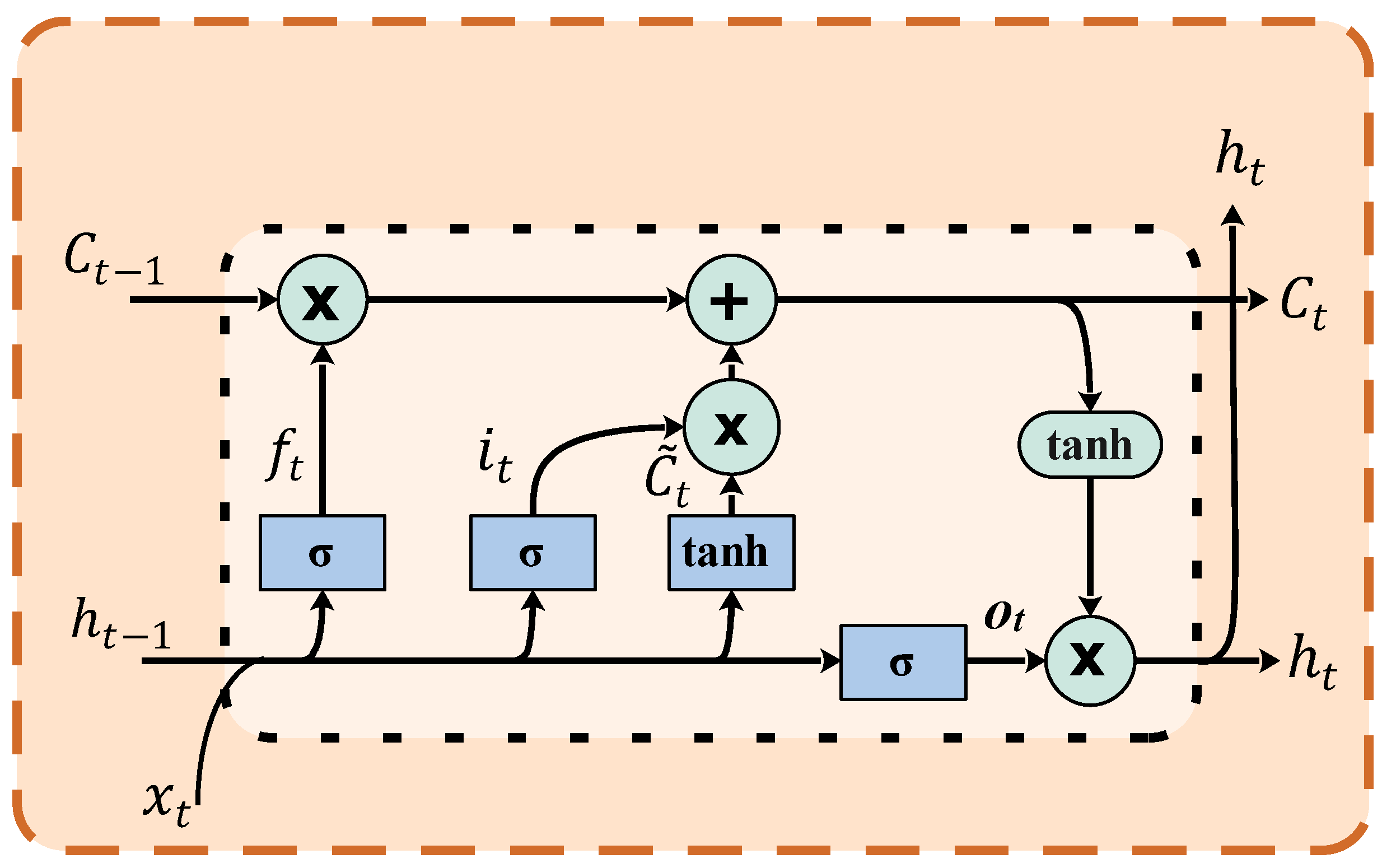
Long short-term memory (LSTM) is a specific type of RNN that addresses the issue of vanishing gradients, which can occur when training traditional RNNs on long sequences. LSTM networks are capable of learning long-term dependencies in sequential data by introducing memory cells and gating mechanisms. The LSTM network is an architecture within RNNs that can effectively capture order dependencies in nonlinear sequence prediction problems. It exhibits the ability to retain information for extended periods. Instead of traditional hidden layers, the core component of the LSTM network is the memory cell. While RNNs have recurrent cells, LSTM cells are equipped with input, output, and forget gates that interact with the cell, in contrast to a single gate found in conventional RNNs. These gates control the flow of information into and out of the cell, allowing the cell to remember values over arbitrary time intervals. By considering the previous state, available memory, and current input, the LSTM network can selectively activate and update cells [43]. One significant advantage of LSTM networks is their ability to mitigate the vanishing gradient problem that often arises in training conventional RNNs. The architecture depicted in Figure 10 effectively addresses this issue, enabling the neural network to retain information over long distances. Consequently, LSTM networks are highly suitable for tasks involving time-series data, such as classification, processing, and making predictions, where significant events in the series may be separated by unknown time intervals. Compared to RNNs, hidden Markov models, and other sequence learning methods, LSTM networks offer relative insensitivity to the duration of gaps, which proves advantageous in many applications [44].
Figure 10 illustrates the process of determining new information to be incorporated into the cell. This involves multiplying the input data with the output of the input gate. Similarly, to calculate the information that can be propagated through the network, the output data of the network is multiplied by the activation of the output gate. Additionally, the decision of whether to forget the previous cell state is determined by multiplying the cell states from the previous time step with the activation of the forget gate.
The operational procedure of the LSTM can be described as follows. To start, let us establish the notations employed in LSTM:
  • x t represents the input at time step t .
  • h t denotes the hidden state at time step t .
  • C t represents the cell state at time step t .
  • W x i , W x f , W x o , and W x g denote the weight matrices for the input x t at time step t associated with the input gate, forget gate, output gate, and candidate cell state, respectively.
  • W h i , W h f , W h o , and W h g represent the weight matrices for the hidden state h t 1 at time step t 1 associated with the input gate, forget gate, output gate, and candidate cell state, respectively.
  • b i , b f , b o , and b g denote the bias vectors for the input gate, forget gate, output gate, and candidate cell state, respectively.
Let us delve into the equations that govern the operations of an LSTM network [45]:
At each time step, an LSTM cell receives an input vector x t and the hidden state vector from the previous time step, h t 1 . The LSTM cell performs a series of computations to update its internal memory and produce an output for the current time step.
 (i) 
Input gate ( i t )
The input gate controls how much of the current input x t and the previous hidden state h t 1 should be stored in the cell state C t . It is calculated using the sigmoid activation function as
i t = σ ( W x i x t + W h i h t 1 + b i )
where σ denotes the sigmoid function.
 (ii) 
Forget gate ( f t )
The forget gate determines how much of the previous cell state C t 1 should be retained or forgotten. It is calculated using the sigmoid activation function as
f t = σ ( W x f x t + W h f h t 1 + b f )
 (iii) 
Output gate ( o t )
The output gate controls how much of the updated cell state C t should be exposed as the hidden state h t . It is calculated using the sigmoid activation function as
o t = σ ( W x o x t + W h o h t 1 + b o )
 (iv) 
Candidate cell state ( C ~ t )
The candidate cell state represents the new information that can be added to the cell state C t . It is calculated using the hyperbolic tangent ( t a n h ) activation function as
C ~ t = t a n h ( W x g x t + W h g h t 1 + b g )
 (v) 
Cell state update ( C t )
The cell state is updated by combining the previous cell state C t 1 with the new information from the input gate ( i t ) and the candidate cell state ( C ~ t ). The update equation is
C t = f t C t 1 + i t C ~ t
where denotes element-wise multiplication.
 (vi) 
Hidden state ( h t )
The hidden state is the output of the LSTM at each time step and is based on the updated cell state C t . It is calculated by applying the t a n h activation function to the cell state ( C t ) and multiplying it by the output gate ( o t ):
h t = o t t a n h ( C t )
These equations govern the operations of an LSTM network. By incorporating memory cells, input gates, forget gates, and output gates, LSTM networks can effectively capture and utilize long-term dependencies in sequential data.

3.7. Performance Metrics for Classification

The dataset used in this study, consisting of color fundus images, is divided randomly into two independent datasets: 80% for training and 20% for testing. To evaluate the performance of the models created for DR disease classification, the study employs the 10-fold cross-validation method. The performance of each classification model is calculated by averaging the accuracy values obtained from each fold. The study measures the performances of all classification models on the test data using the metrics defined in Equations (51)–(54). These metrics, which are derived from the confusion matrix, utilize the symbols T P (true positives), F P (false positives), T N (true negatives), and F N (false negatives).
A c c u r a c y = T P + T N T P + T N + F P + F N   ,  
P r e c i s i o n = T P T P + F P   ,
R e c a l l = T P T P + F N   ,
F 1 s c o r e = 2 × R e c a l l × P r e c i s i o n R e c a l l + P r e c i s i o n   .
A c c u r a c y is a metric used to measure how often a classifier makes correct predictions. It is calculated by dividing the number of correct predictions by the total number of predictions. A c c u r a c y provides an overall assessment of the classifier’s performance. P r e c i s i o n is the ratio of correctly predicted positive samples to the total number of positive predictions made by the classifier. It is calculated by dividing the number of true positive predictions by the sum of true positives and false positives. P r e c i s i o n reflects the classifier’s ability to make accurate positive predictions. R e c a l l , also known as sensitivity, is a measure of the proportion of actual positive samples that are correctly identified as positive by the classifier. It is calculated by dividing the number of true positive predictions by the sum of true positives and false negatives. R e c a l l indicates the classifier’s ability to identify positive samples correctly. F 1 s c o r e combines both recall and precision into a single metric. It is the harmonic mean of recall and precision and provides a balanced assessment of the classifier’s performance. F 1 s c o r e is particularly useful when there is an imbalance between the number of positive and negative samples in the dataset [46].

3.8. Framework of the Proposed DR Disease Classification Model

In this study, we propose a robust hybrid model that can classify DR disease with low computational cost, minimum model complexity, and high accuracy by dealing with nonlinear dynamics in the image. The framework of the proposed model is illustrated in Figure 11, and the processing steps are briefly outlined below.
Step 1: Data preparation involves randomly dividing the dataset, which contains images from each DR disease class, as well as the healthy class, into two independent datasets. Eighty percent of the data is allocated for the training phase, while the remaining twenty percent is reserved for the test phase. Fractal analysis is used to uncover the presence of chaos in the images belonging to each DR disease class, as well as the healthy class.
Step 2: Employing 2D-SWT for signal processing, the feature groups are obtained for each wavelet family by applying 2D-SWT using biorthogonal, Coiflet, Daubechies, Fejer–Korovkin, reverse biorthogonal, and symlet wavelet families to the dataset that comprises images from each DR disease class, as well as the healthy class. Following a three-level decomposition, a total of 12 image matrices are derived, consisting of vertical, horizontal, diagonal, and approximate matrices.
Step 3: The feature extraction process includes extracting entropy- and statistical-based features from the vertical, horizontal, diagonal, and approximate matrices obtained through 2D-SWT. The following eight features, namely entropy, Renyi entropy, Shannon entropy, energy, arithmetic mean, standard deviation, kurtosis, and skewness, are applied to these four matrices. This procedure is repeated for the second- and third-level decomposition in 2D-SWT. As a result of this step, a total of 96 features are extracted. These extracted features encompass the nonlinear dynamics that represent the classes of DR disease.
Step 4: In the feature selection stage using CPSO-kNN, a wrapper approach is utilized, combining the CPSO and kNN algorithms, to select features that minimize computational complexity, address chaos in fundus images, and ensure high model performance. The fitness function is constructed to meet these criteria. The effectiveness of various chaotic maps is tested to enhance the convergence speed and optimal solution of the optimization algorithm, and the most suitable one is integrated into the optimization process to achieve the highest classification accuracy with the least number of features. The extracted features for each wavelet family are subjected to normalization, and the most appropriate ones are selected.
Step 5: In the classification stage with RNN-LSTM, the selected optimum feature vectors are finally fed into the RNN-LSTM for classifying DR disease sub-types like PDR, mild NPDR, moderate NPDR, and severe NPDR, as well as healthy cases. The classification performance of the model is evaluated using metrics such as accuracy, precision, recall, and F1-score, and its effectiveness is compared to the SVM classifier.

4. Results and Discussion

This section includes studies that exhibit the classification effectiveness of the proposed model on a dataset comprising color fundus images. The dataset contains disease classes such as mild NPDR, moderate NPDR, severe NPDR, and PDR, as well as the healthy class. The presence of chaos in the dataset is revealed by fractal dimension analysis. The proposed model involves a three-level 2D-SWT technique based on the ‘bior2.8’ wavelet family, the CPSO and kNN wrapper approach based on the logistic chaotic map, and the RNN-LSTM network. The impact of the features selected through the chaotic wrapper approach on the model’s performance is analyzed for each wavelet family. The performance of our model built with the RNN-LSTM network is compared with the performance of the model built with SVM.

4.1. Dataset

In this study, an experimentally prepared publicly available dataset for DR classification known as APTOS 2019 was used [47]. The dataset comprises color fundus images categorized into five classes, namely healthy, mild NPDR, moderate NPDR, severe NPDR, and PDR, as depicted in Figure 12. The dataset was split into two groups using the holdout method: 80% of the data was allocated for the training phase, while the remaining 20% was reserved for the test phase. This division was performed randomly and independently. The training dataset consists of 10,000 color fundus images, with 2000 images from each class, while the test dataset consists of 2500 color fundus images, with 500 images from each class. In total, 12,500 color fundus image data were employed for the study. The size of each image in the dataset was reduced to 512 × 512 pixels in order to overcome the problems of limited memory and computational cost during the training phase of the model.

4.2. Fractal Dimension Analysis with Fourier Power Spectrum

The lesions and vessels in the original color fundus image were revealed using the green channel image. The aim here is to enhance the visibility of surface density in both lesions and vessels. Fractal theory can be employed to assess surface intensity by representing pixels that exhibit self-similarity across various scales. In the absence of lesions, the fractal dimension of the surface is smaller compared to a surface that includes lesions.
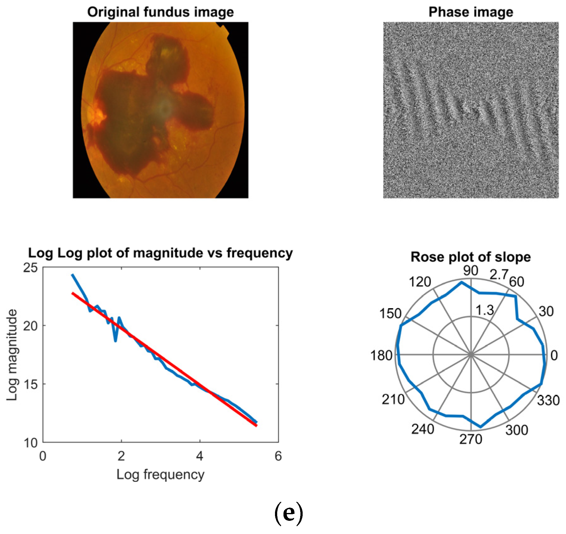
The fractal pattern present in the image is identified by the fractal dimension derived from the Fourier power spectrum. The fractal Fourier method is used to determine the fractal dimension of an image. Fast Fourier transform is applied to the images in 24 different directions, using 30-degree angles. The resulting average power spectrum ( F ) is a function of frequency ( f ). This function satisfies the following relationships:
F f 2 β
β = 2 H n + 2
where H n represents the Hurst coefficient [48]. The curve of the resulting power spectrum versus frequency is plotted on a log-log scale for each class in Figure 13. Here, a curve is fitted using linear regression versus the plotted curve, and β is obtained from the slope of this curve. The fractal dimension ( F D ) of the image is calculated using the obtained β value as follows:
F D = 6 + β 2
A total of 24 slopes are derived from the graphs presented in Figure 13, as 24 different directions are utilized in power spectrum analysis. The average of these 24 slopes is then calculated to determine the fractal dimension for each class using Equation (57). The measured fractal dimensions for each class are as follows: 1.49 for the healthy, 1.58 for mild NPDR, 1.62 for moderate NPDR, 1.72 for severe NPDR, and 1.79 for PDR. When Figure 13 and the measured fractal dimensions are evaluated together, it is observed that the fractal dimension increases depending on the severity of the disease. The increase in fractal dimension indicates an increase in the complexity of the image. The obtained findings indicate that the dataset utilized exhibits fractal behavior and reveals the existence of nonlinear dynamics that vary based on the severity of the disease.

4.3. Feature Extraction Applying 2D-SWT with Wavelet Families

The features of DR diseases are extracted using 2D-SWT with various wavelet families, including biorthogonal, Coiflet, Daubechies, Fejer–Korovkin, reverse biorthogonal, and symlet. The filter lengths for each wavelet family are specified in Table 2. The original image matrix of size 512 × 512 pixels undergoes a three-level decomposition. This decomposition yields image matrices for vertical, horizontal, diagonal, and approximation coefficients for each wavelet family. It is noted that the size of the resulting image matrices is 512 × 512 .
In the study, entropy- and statistical-based features were utilized to achieve accurate classification of DR diseases. The entropy- and statistical-based features listed in Table 3 were applied to the image matrices, I = I 1 V , I 1 H , I 1 D , I 1 A , I 2 V , I 2 H , I 2 D , I 2 A , I 3 V , I 3 H , I 3 D , I 3 A , obtained from the first-, second-, and third-level decompositions for each wavelet family. A total of 96 features were extracted, and each feature was labeled as shown in Table 4.

4.4. Feature Selection with CPSO-kNN

The 2D-SWT method is utilized to generate 12 image matrices and extract features. Prior to directly employing these feature groups in the classification stage, it is crucial to identify the most suitable subset of features that can maintain high performance while minimizing model complexity. Inspired by the social interactions and swarm behavior of birds, the CPSO algorithm is used to select the most suitable features for each wavelet family from the normalized feature set with the help of chaotic maps. This selection process aims to maintain the high performance of the kNN classifier. This selection process is guided by the fitness function denoted as
f i t n e s s = μ × e r + σ × s e l e c t e d   f e a t u r e   s u b s e t t o t a l   n u m b e r   o f   f e a t u r e s
where e r represents the classification error of the kNN classifier. The significance of classification quality and subset length is represented by μ and σ , respectively. In this context, μ takes values between 0 and 1 , while σ is calculated as ( 1 μ ) . The fitness function takes into account both the number of features utilized in the model and the model’s performance. By considering these factors, the fitness function aims to minimize model complexity and computational cost. The parameter values for the CPSO-kNN wrapper approach employed in the study are provided in Table 5. It is important to highlight that the feature selection process in the models constructed for each wavelet family is conducted based on the parameter values outlined in Table 5.
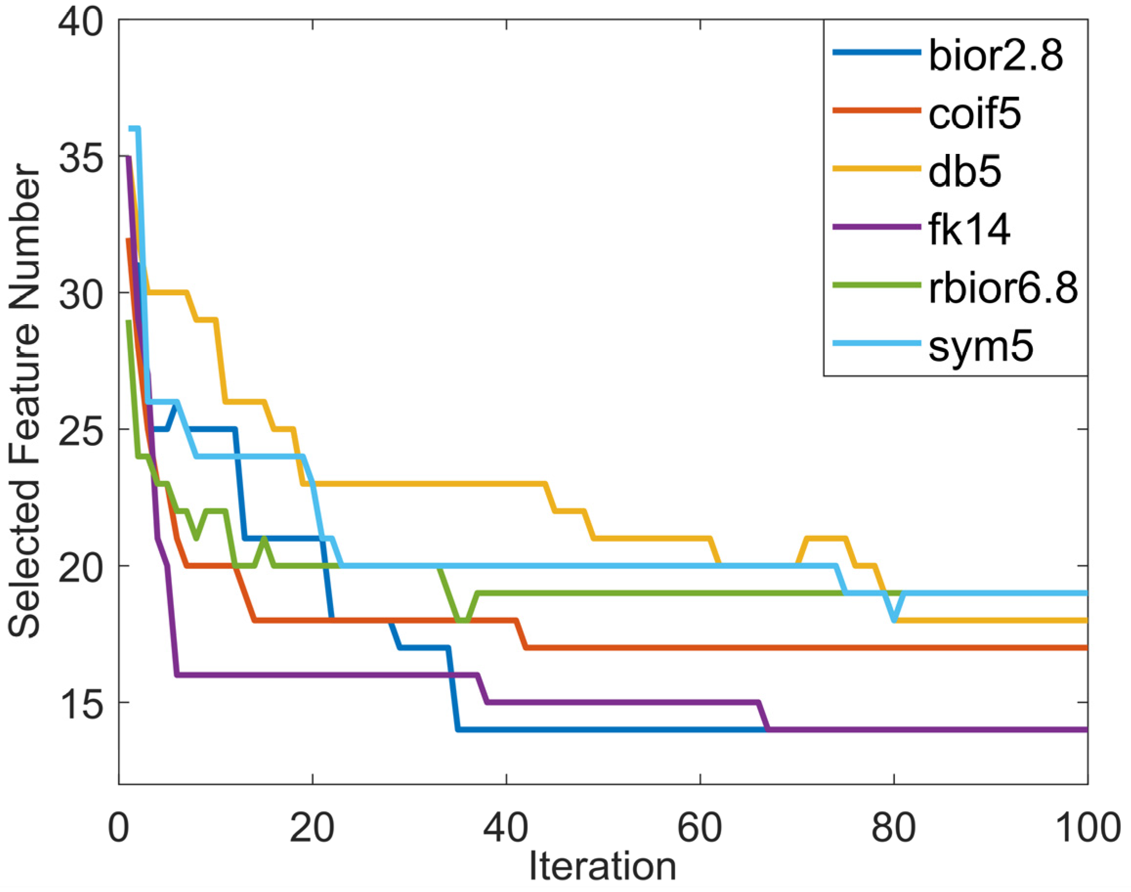
The number of features selected during iteration for the wavelet families with the highest performance with the CPSO-kNN wrapper approach is illustrated in Figure 14. It can be said that the best performance is obtained for the ‘bior2.8’ wavelet family. As the iteration progresses, it is observed that the number of selected features decreases. It is noteworthy that the convergence speed of CPSO in selecting features that maintain high model performance is higher compared to other wavelet families when extracting features using the ‘bior2.8’ wavelet family. It should be noted that this condition reduces the complexity of the model.
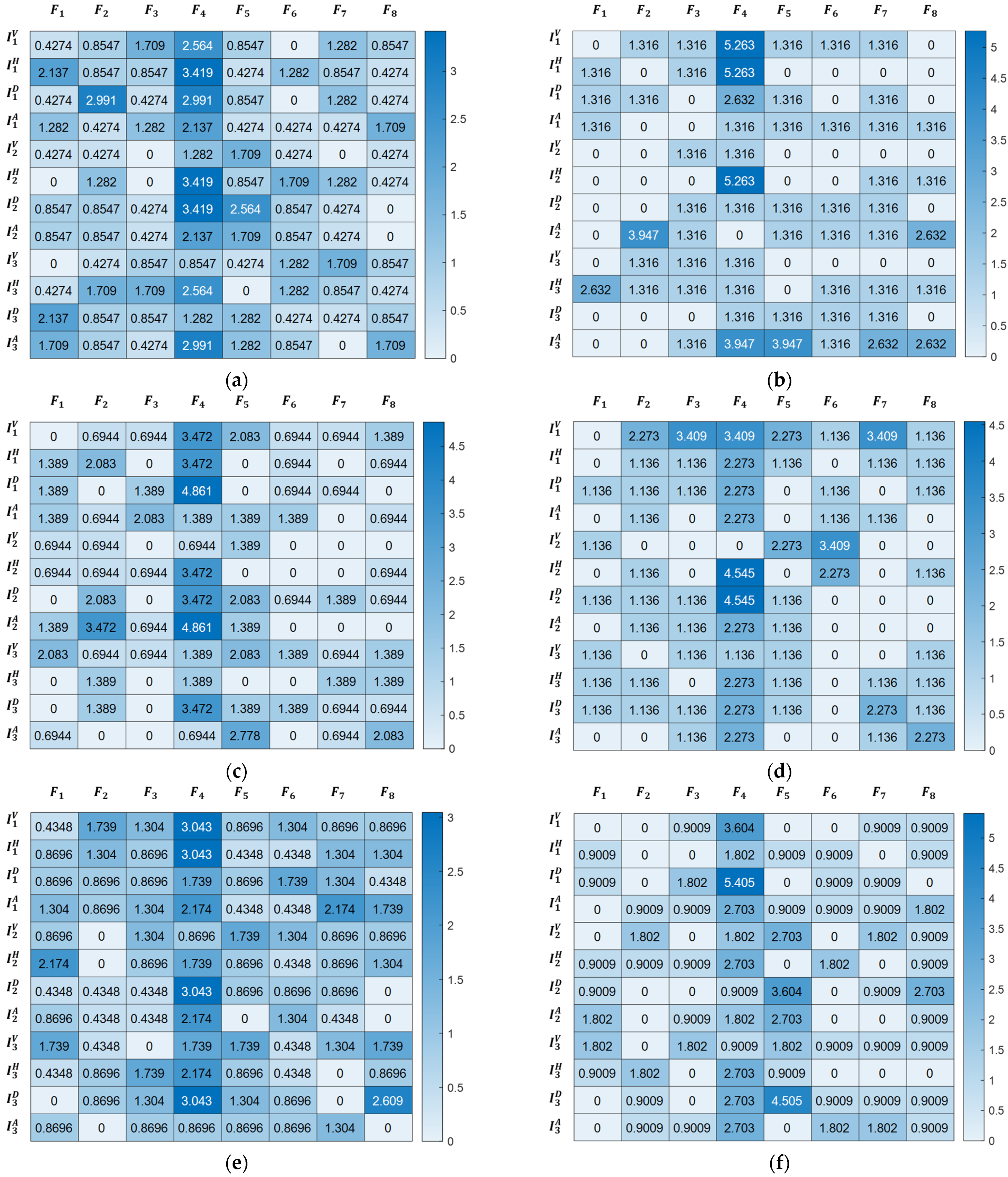
The heat map in Figure 15 shows the percentage of total selection rates for the best feature groups obtained from the biorthogonal, Coiflet, Daubechies, Fejer–Korovkin, reverse biorthogonal, and symlet wavelet families after 100 iterations in CPSO. The analysis of the 12 image matrices obtained from 2D-SWT reveals that the highest number of features was extracted from I 1 H , I 2 H , and I 2 D for the biorthogonal wavelet family, I 1 V , I 1 H , and I 2 H for the Coiflet wavelet family, I 1 D and I 2 A for the Daubechies wavelet family, I 2 H and I 2 D for the Fejer–Korovkin wavelet family, I 1 V , I 1 H , I 2 D , and I 3 D for the reverse biorthogonal wavelet family, and I 1 D for the Symlet wavelet family.
The feature F 4 , which is one of the statistical-based features, is selected in at least 25% of all wavelet families. In addition to the F 4 feature, F 1 , F 2 , and F 5 for the biorthogonal, F 3 , F 5 , and F 7 for the Coiflet, F 2 and F 5 for the Daubechies, F 2 , F 3 , F 5 , F 7 , and F 8 for the Fejer–Korovkin, F 1 , F 3 , F 5 , F 6 , F 7 , and F 8 for the reverse biorthogonal, and F 5 and F 8 for the symlet are selected in at least 10%. However, in the DR disease model, the feature F 8 for the biorthogonal wavelet family, F 1 for the Coiflet wavelet family, F 3 for the Daubechies wavelet family, F 1 for the Fejer–Korovkin wavelet family, F 2 for the reverse biorthogonal wavelet family, and F 2 for the symlet wavelet family are employed the least. The selection rate for these features ranges approximately between 6% and 8%.

4.5. Evaluation and Discussion of Classification Models

All the models discussed in the study were executed on a personal computer equipped with an Intel Core i7-12700H CPU, a 6 GB NVIDIA GeForce RTX 3060 graphics card, and 16 GB of RAM. All the codes were compiled using MATLAB 2022b. The models developed in the study were tested on a dataset of 2500 samples belonging to five different classes. Each model was run 50 times, and the performance was evaluated in terms of mean and standard deviation. The study investigated the influence of both the optimization algorithm and the classifier algorithms on the performance of the model. The parameter values for the proposed classifier algorithm are provided in Table 6.
The effect of using the CPSO algorithm with the 10 chaotic maps listed in Table 1 on the performance of the model was investigated. The wavelet family that yielded the best performance for each chaotic map is presented in Table 7. Models built using selected features extracted from the reverse biorthogonal wavelet family, utilizing Chebyshev, circle, and piecewise chaotic maps, demonstrate the highest performance for the respective maps. Similarly, models built using selected features extracted from the biorthogonal wavelet family utilizing iterative, logistic, and sine chaotic maps exhibit the highest performance for the respective maps. Furthermore, models built using selected features extracted from the Coiflet wavelet family, with Gauss and tent chaotic maps, as well as models created using selected features extracted from the Daubechies wavelet family, with singer and sinusoidal chaotic maps, demonstrate the highest performance for the respective maps. Notably, it is observed that there are no models utilizing features extracted from the Fejer–Korovkin and symlet wavelet families that achieve the highest performance among chaotic maps. The performance of models constructed using RNN-LSTM stands out, exceeding the 99% threshold for all chaotic maps. However, the performance of the models built with SVM is around 94% to 98%. Among all the models created in the study, the architecture that shows the superior performance is the one that feeds RNN-LSTM with selected features generated from the ‘bior2.8’ wavelet family, using the logistic-chaotic-map-based CPSO-kNN approach.
The performance of the RNN-LSTM and SVM classification models, which were created using features selected by the CPSO-kNN wrapper approach based on the logistic chaotic map, was evaluated based on the accuracy metric. The corresponding results are presented in Table 8. When examining all the models in Table 8 in terms of the accuracy performance metric, it is observed that the model including the three-level 2D-SWT technique based on the ‘bior2.8’ wavelet family, the wrapper approach consisting of logistic-chaotic-map-based CPSO and kNN, and the RNN-LSTM network exhibited the highest performance. Therefore, this model is proposed for DR disease classification. The performance of the proposed model was measured as 99.64%. Furthermore, the low standard deviation confirms the robustness of the model.
Fourteen subsets of features generated from the 2D-SWT technique based on the ‘bior2.8’ wavelet family were selected for the proposed classification model of DR disease using the CPSO-kNN wrapper approach. Among the selected features for the proposed model, it is observed that arithmetic mean, skewness, kurtosis, and Shannon-entropy-based features are the most frequently selected. Additionally, it is noteworthy that half of the selected features were extracted from the third-level decomposition. This finding provides an explanation for why three-level decomposition was utilized in the study. The selection of the least number of features while achieving the highest classification performance with the proposed model structure also demonstrates the capability of the optimization process to cope with nonlinear dynamics.
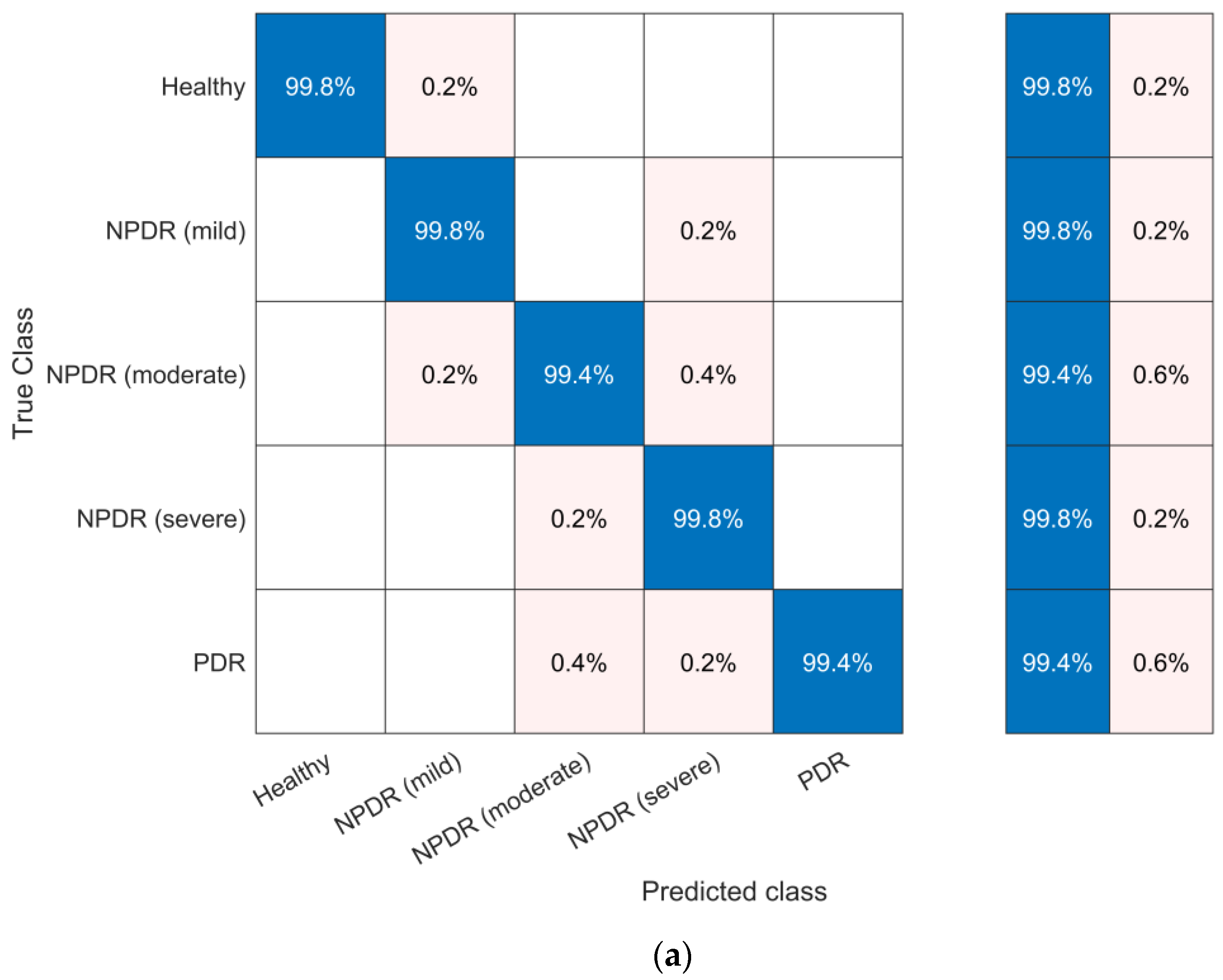
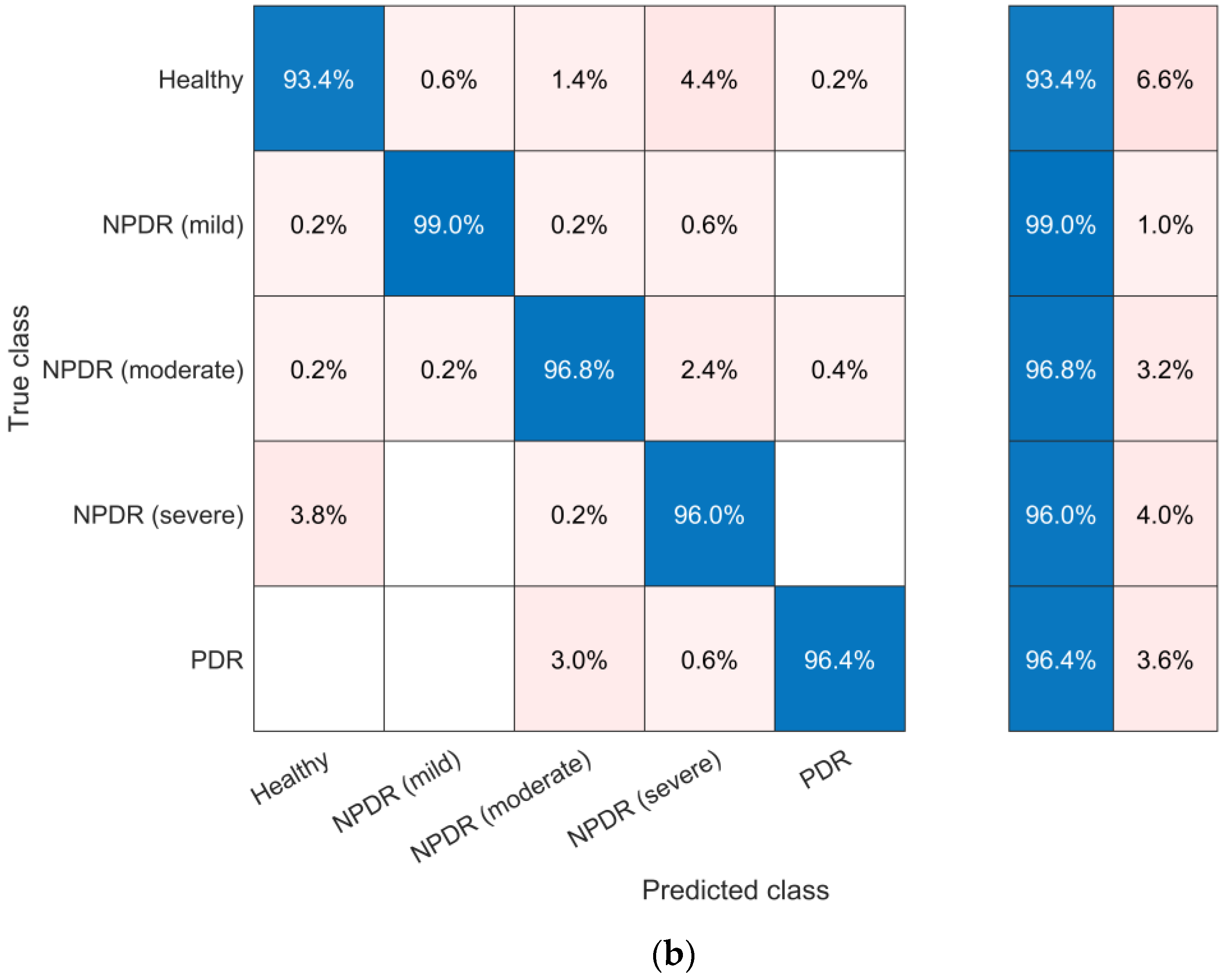
The confusion matrix for the proposed RNN-LSTM and SVM classifiers in the study, depicting the classification of healthy, mild NPDR, moderate NPDR, severe NPDR, and PDR, is presented in Figure 16. When examining Figure 16, it can be observed that the model built with the RNN-LSTM classifier achieves a classification performance of 99.8% for healthy cases, 99.8% for mild NPDR, 99.4% for moderate NPDR, 99.8% for severe NPDR, and 99.4% for PDR. On the other hand, the model built with the SVM classifier achieves a classification performance of 93.4% for healthy cases, 99.0% for mild NPDR, 96.8% for moderate NPDR, 96.0% for severe NPDR, and 96.4% for PDR. It can be said that the model constructed with the SVM classifier misclassified color fundus images into two or more incorrect classes for each class, indicating a serious threat to the reliability of the model.
The performance of models constructed with the RNN-LSTM and SVM classifiers for the ‘bior2.8’ wavelet family and logistic chaotic map was evaluated using multiple metrics such as precision, recall, F1-score, and accuracy. These results are provided in Table 9.
The results in Table 9 demonstrate that the proposed DR disease classification model effectively handles nonlinear dynamics and exhibits superior performance in terms of all metrics used in the study. Experimental findings indicate that our model, with low computational complexity, accurately classifies DR disease grades with high performance. This confirms the feasibility of applying our model in real-time scenarios.

5. Conclusions

The development of an effective and accurate model for diagnosing and classifying DR disease is of utmost importance in order to prevent irreversible vision loss and blindness in diabetic patients. This study addresses this critical issue by proposing a robust AI-based model that overcomes the nonlinear dynamics of DR through low computational complexity and high classification accuracy. The proposed model follows a four-stage process incorporating fractal analysis, 2D-SWT, feature extraction using entropy and statistical functions, a chaotic-based wrapper approach, and an RNN-LSTM architecture. Several significant contributions are highlighted in this study. Fractal analysis is utilized to identify chaos in the images of each DR disease class and healthy cases. The application of the 2D-SWT helps extract feature groups for each wavelet family, revealing characteristic features of DR disease. Entropy- and statistical-based features are then extracted from the image matrices obtained through 2D-SWT, capturing the nonlinear dynamics representing the DR disease classes. To select features that maintain high model performance while minimizing computational complexity and addressing chaoticity in color fundus images, a wrapper approach combining CPSO and kNN algorithms is employed. The effectiveness of various chaotic maps is evaluated, and the most suitable one is integrated into the optimization process to achieve the highest classification accuracy with minimal features. Finally, the RNN-LSTM architecture is utilized for classifying DR disease sub-types and healthy cases. The proposed model’s performance is evaluated using metrics such as accuracy, precision, recall, and F1-score and is compared to the SVM classifier. The results obtained from extensive experiments demonstrate that the proposed model effectively copes with the nonlinear dynamics in color fundus images while maintaining low computational complexity. The model achieves precise diagnosis and classification of all stages of DR disease, including mild NPDR, moderate NPDR, severe NPDR, PDR, and cases with no DR. The model’s robustness is confirmed through 10-fold cross-validation. The proposed model, incorporating three-level 2D-SWT using the ‘bior2.8’ wavelet family, a chaotic-based wrapper approach (using a logistic-chaotic-map-based CPSO and kNN), and an RNN-LSTM network, demonstrates the best performance for the DR disease classification. Experimental results affirm that the proposed model effectively addresses nonlinear dynamics, offers low computational complexity, and can be applied in real-time scenarios. In conclusion, the developed AI-based model presents a significant advancement in the early diagnosis and classification of DR disease through fundus image analysis. By effectively overcoming nonlinear dynamics and ensuring low computational complexity, the model provides real-time, end-to-end classification, enabling timely intervention and prevention of vision loss in diabetic patients. The findings of this study contribute to improving healthcare practices and hold promising potential for enhancing the diagnosis and management of DR globally.

Author Contributions

Conceptualization, A.A.; methodology, Y.B.Ö. and A.A.; software, Y.B.Ö. and A.A.; writing—original draft, Y.B.Ö. and A.A.; writing—review and editing, A.A.; supervision, A.A. All authors have read and agreed to the published version of the manuscript.

Funding

This research received no external funding.

Data Availability Statement

The data presented in this study are available upon request from the corresponding author.

Acknowledgments

This research is supported by Zonguldak Bülent Ecevit University (BAP Project No: 2021–75737790-03). The authors would like to thank Zonguldak Bülent Ecevit University for their support.

Conflicts of Interest

The authors declare no conflict of interest.

References

  1. Saeedi, P.; Petersohn, I.; Salpea, P.; Malanda, B.; Karuranga, S.; Unwin, N.; Colagiuri, S.; Guariguata, L.; Motala, A.A.; Ogurtsova, K.; et al. Global and regional diabetes prevalence estimates for 2019 and projections for 2030 and 2045: Results from the International Diabetes Federation Diabetes Atlas. Diabetes Res. Clin. Pract. 2019, 157, 107843. [Google Scholar] [CrossRef] [Green Version]
  2. Wong, T.Y.; Cheung, C.M.G.; Larsen, M.; Sharma, S.; Simó, R. Diabetic retinopathy (Primer). Nat. Rev. Dis. Primers 2016, 2, 16012. [Google Scholar] [CrossRef] [PubMed]
  3. Zago, G.T.; Andreão, R.V.; Dorizzi, B.; Salles, E.O.T. Diabetic retinopathy detection using red lesion localization and convolutional neural networks. Comput. Biol. Med. 2020, 116, 103537. [Google Scholar] [CrossRef] [PubMed]
  4. Lee, R.; Wong, T.Y.; Sabanayagam, C. Epidemiology of diabetic retinopathy, diabetic macular edema and related vision loss. Eye Vis. 2015, 2, 1–25. [Google Scholar] [CrossRef] [Green Version]
  5. Kobrin Klein, B.E. Overview of epidemiologic studies of diabetic retinopathy. Ophthalmic Epidemiol. 2007, 14, 179–183. [Google Scholar] [CrossRef] [PubMed]
  6. Wan, S.; Liang, Y.; Zhang, Y. Deep convolutional neural networks for diabetic retinopathy detection by image classification. Comput. Electr. Eng. 2018, 72, 274–282. [Google Scholar] [CrossRef]
  7. Nazir, T.; Irtaza, A.; Shabbir, Z.; Javed, A.; Akram, U.; Mahmood, M.T. Diabetic retinopathy detection through novel tetragonal local octa patterns and extreme learning machines. Artif. Intell. Med. 2019, 99, 101695. [Google Scholar] [CrossRef]
  8. Aiello, L.M. Perspectives on diabetic retinopathy. Am. J. Ophthalmol. 2003, 136, 122–135. [Google Scholar] [CrossRef]
  9. Stratton, I.M.; Kohner, E.M.; Aldington, S.J.; Turner, R.C.; Holman, R.R.; Manley, S.E.; Matthews, D.R. for the UKPDS Group. UKPDS 50: Risk factors for incidence and progression of retinopathy in type II diabetes over 6 years from diagnosis. Diabetologia 2001, 44, 156–163. [Google Scholar] [CrossRef] [Green Version]
  10. Wu, B.; Zhu, W.; Shi, F.; Zhu, S.; Chen, X. Automatic detection of microaneurysms in retinal fundus images. Comput. Med. Imaging Graph. 2017, 55, 106–112. [Google Scholar] [CrossRef]
  11. García, M.; Sánchez, C.I.; López, M.I.; Abásolo, D.; Hornero, R. Neural network-based detection of hard exudates in retinal images. Comput. Methods Programs Biomed. 2009, 93, 9–19. [Google Scholar] [CrossRef] [Green Version]
  12. Faust, O.; Acharya U, R.; Ng, E.Y.K.; Ng, K.H.; Suri, J.S. Algorithms for the automated detection of diabetic retinopathy using digital fundus images: A review. J. Med. Syst. 2012, 36, 145–157. [Google Scholar] [CrossRef]
  13. Bilal, A.; Zhu, L.; Deng, A.; Lu, H.; Wu, N. AI-based automatic detection and classification of diabetic retinopathy using U-Net and deep learning. Symmetry 2022, 14, 1427. [Google Scholar] [CrossRef]
  14. Math, L.; Fatima, R. Adaptive machine learning classification for diabetic retinopathy. Multimed. Tools Appl. 2021, 80, 5173–5186. [Google Scholar] [CrossRef]
  15. Qiao, L.; Zhu, Y.; Zhou, H. Diabetic retinopathy detection using prognosis of microaneurysm and early diagnosis system for non-proliferative diabetic retinopathy based on deep learning algorithms. IEEE Access 2020, 8, 104292–104302. [Google Scholar] [CrossRef]
  16. Gadekallu, T.R.; Khare, N.; Bhattacharya, S.; Singh, S.; Maddikunta, P.K.R.; Ra, I.H.; Alazab, M. Early detection of diabetic retinopathy using PCA-firefly based deep learning model. Electronics 2020, 9, 274. [Google Scholar] [CrossRef] [Green Version]
  17. Kukkar, A.; Gupta, D.; Beram, S.M.; Soni, M.; Singh, N.K.; Sharma, A.; Neware, R.; Shabaz, M.; Rizwan, A. Optimizing deep learning model parameters using socially implemented IoMT systems for diabetic retinopathy classification problem. IEEE Trans. Comput. Soc. Syst. 2022. Early Access. [Google Scholar]
  18. Gundluru, N.; Rajput, D.S.; Lakshmanna, K.; Kaluri, R.; Shorfuzzaman, M.; Uddin, M.; Rahman Khan, M.A. Enhancement of detection of diabetic retinopathy using Harris hawks optimization with deep learning model. Comput. Intell. Neurosci. 2022, 2022, 8512469. [Google Scholar] [CrossRef] [PubMed]
  19. Uppamma, P.; Bhattacharya, S. Diabetic retinopathy detection: A blockchain and African vulture optimization algorithm-based deep learning framework. Electronics 2023, 12, 742. [Google Scholar] [CrossRef]
  20. Gupta, S.; Thakur, S.; Gupta, A. Optimized hybrid machine learning approach for smartphone based diabetic retinopathy detection. Multimed. Tools Appl. 2022, 81, 14475–14501. [Google Scholar] [CrossRef]
  21. Beevi, S.Z. Multi-Level severity classification for diabetic retinopathy based on hybrid optimization enabled deep learning. Biomed. Signal Process. Control 2023, 84, 104736. [Google Scholar] [CrossRef]
  22. Rachapudi, V.; Rao, K.S.; Rao, T.S.M.; Dileep, P.; Deepika Roy, T.L. Diabetic retinopathy detection by optimized deep learning model. Multimed. Tools Appl. 2023, 82, 27949–27971. [Google Scholar] [CrossRef]
  23. Williams, J.R.; Amaratunga, K. Introduction to wavelets in engineering. Int. J. Numer. Methods Eng. 1994, 37, 2365–2388. [Google Scholar] [CrossRef] [Green Version]
  24. Kim, C.H.; Aggarwal, R. Wavelet transforms in power systems. Part 1: General introduction to the wavelet transforms. Power Eng. J. 2000, 14, 81–87. [Google Scholar]
  25. Mallat, S. A Wavelet Tour of Signal Processing, 2nd ed.; Elsevier: Berkeley, CA, USA, 1999; ISBN 978-0-12-466606-1. [Google Scholar]
  26. Nason, G.P.; Silverman, B.W. The discrete wavelet transform in S. J. Comput. Graph. Stat. 1994, 3, 163–191. [Google Scholar]
  27. Vetterli, M.; Herley, C. Wavelets and filter banks: Theory and design. IEEE Trans. Signal Process. 1992, 40, 2207–2232. [Google Scholar] [CrossRef] [Green Version]
  28. Nason, G.P.; Silverman, B.W. The stationary wavelet transform and some statistical applications. In Wavelets and Statistics; Springer: New York, NY, USA, 1995; pp. 281–299. [Google Scholar]
  29. Pesquet, J.C.; Krim, H.; Carfantan, H. Time-invariant orthonormal wavelet representations. IEEE Trans. Signal Process. 1996, 44, 1964–1970. [Google Scholar] [CrossRef] [Green Version]
  30. Merah, M.; Abdelmalik, T.A.; Larbi, B.H. R-peaks detection based on stationary wavelet transform. Comput. Methods Programs Biomed. 2015, 121, 149–160. [Google Scholar] [CrossRef]
  31. Mallat, S.G. A theory for multiresolution signal decomposition: The wavelet representation. IEEE Trans. Pattern Anal. Mach. Intell. 1989, 11, 674–693. [Google Scholar] [CrossRef] [Green Version]
  32. Keinert, F. Biorthogonal wavelets for fast matrix computations. Appl. Comput. Harmon. Anal. 1994, 1, 147–156. [Google Scholar] [CrossRef] [Green Version]
  33. Monzón, L.; Beylkin, G.; Hereman, W. Compactly supported wavelets based on almost interpolating and nearly linear phase filters (coiflets). Appl. Comput. Harmon. Anal. 1999, 7, 184–210. [Google Scholar] [CrossRef] [Green Version]
  34. Daubechies, I. Ten Lectures on Wavelets; Society for Industrial and Applied Mathematics: Philadelphia, PA, USA, 1992; ISBN 0-89871-274-2. [Google Scholar]
  35. Daubechies, I. Orthonormal bases of compactly supported wavelets. Commun. Pure Appl. Math. 1988, 41, 909–996. [Google Scholar] [CrossRef] [Green Version]
  36. Daubechies, I. The wavelet transform, time-frequency localization and signal analysis. IEEE Trans. Inf. Theory 1990, 36, 961–1005. [Google Scholar] [CrossRef] [Green Version]
  37. Nielsen, M. On the construction and frequency localization of finite orthogonal quadrature filters. J. Approx. Theory 2001, 108, 36–52. [Google Scholar] [CrossRef] [Green Version]
  38. Szewczyk, R.; Grabowski, K.; Napieralska, M.; Sankowski, W.; Zubert, M.; Napieralski, A. A reliable iris recognition algorithm based on reverse biorthogonal wavelet transform. Pattern Recognit. Lett. 2012, 33, 1019–1026. [Google Scholar] [CrossRef]
  39. Yang, C.; Liu, P.; Yin, G.; Jiang, H.; Li, X. Defect detection in magnetic tile images based on stationary wavelet transform. NDT E Int. 2016, 83, 78–87. [Google Scholar] [CrossRef]
  40. Kennedy, J.; Eberhart, R. Particle swarm optimization. In Proceedings of the ICNN’95 International Conference on Neural Networks, Perth, Australia, 27 November–1 December 1995. [Google Scholar]
  41. dos Santos Coelho, L.; Herrera, B.M. Fuzzy identification based on a chaotic particle swarm optimization approach applied to a nonlinear yo-yo motion system. IEEE Trans. Ind. Electron. 2007, 54, 3234–3245. [Google Scholar] [CrossRef]
  42. Wei, D.; Wang, B.; Lin, G.; Liu, D.; Dong, Z.; Liu, H.; Liu, Y. Research on unstructured text data mining and fault classification based on RNN-LSTM with malfunction inspection report. Energies 2017, 10, 406. [Google Scholar] [CrossRef] [Green Version]
  43. Karasu, S.; Altan, A. Crude oil time series prediction model based on LSTM network with chaotic Henry gas solubility optimization. Energy 2022, 242, 122964. [Google Scholar] [CrossRef]
  44. Hochreiter, S.; Schmidhuber, J. Long short-term memory. Neural Comput. 1997, 9, 1735–1780. [Google Scholar] [CrossRef]
  45. Hua, Y.; Mou, L.; Zhu, X.X. Recurrently exploring class-wise attention in a hybrid convolutional and bidirectional LSTM network for multi-label aerial image classification. ISPRS J. Photogramm. Remote Sens. 2019, 149, 188–199. [Google Scholar] [CrossRef]
  46. Sokolova, M.; Lapalme, G. A systematic analysis of performance measures for classification tasks. Inf. Process. Manag. 2009, 45, 427–437. [Google Scholar] [CrossRef]
  47. APTOS 2019 Blindness Detection. Available online: https://www.kaggle.com/c/aptos2019-blindness-detection (accessed on 29 June 2023).
  48. Quevedo, R.; Carlos, L.G.; Aguilera, J.M.; Cadoche, L. Description of food surfaces and microstructural changes using fractal image texture analysis. J. Food Eng. 2022, 53, 361–371. [Google Scholar] [CrossRef]
Figure 1. Diabetic retinopathy findings in fundus images: (a) microaneurysms, soft exudates, and neovascularization; (b) intraretinal microvascular abnormality, hard exudates, and hemorrhages.
Fractalfract 07 00598 g001
Figure 2. Three-level decomposition with SWT.
Fractalfract 07 00598 g002
Figure 3. The scaling and wavelet functions of the ‘bior2.8’ wavelet, which yielded the highest classification performance for the biorthogonal wavelet family in the study.
Fractalfract 07 00598 g003
Figure 4. The scaling and wavelet functions of the ‘coif5’ wavelet, which provided the highest classification performance in the Coiflet wavelet family in the study.
Fractalfract 07 00598 g004
Figure 5. The scaling and wavelet functions of the ‘db5’ wavelet, which produced the highest classification performance in the Daubechies wavelet family in the study.
Fractalfract 07 00598 g005
Figure 6. The scaling and wavelet functions of the ‘fk14’ wavelet, given the best classification performance for the Fejer–Korovkin wavelet family in the study.
Fractalfract 07 00598 g006
Figure 7. The scaling and wavelet functions of the ‘rbior6.8’ wavelet that produced the highest classification performance in the reverse biorthogonal wavelet family in the study.
Fractalfract 07 00598 g007
Figure 8. The scaling and wavelet functions of the ‘sym5’ wavelet, which achieved the best classification performance in the symlet wavelet family in the study.
Fractalfract 07 00598 g008
Figure 9. The expanded form of the RNN.
Fractalfract 07 00598 g009
Figure 10. Basic structure of the LSTM.
Fractalfract 07 00598 g010
Figure 11. Framework of the proposed DR disease classification approach.
Fractalfract 07 00598 g011
Figure 12. A sample of the dataset includes DR disease classes such as mild NPDR, moderate NPDR, severe NPDR, PDR, and the healthy class.
Fractalfract 07 00598 g012
Figure 13. Fractal dimension analysis by FFT for (a) healthy, (b) mild NPDR, (c) moderate NPDR, (d) severe NPDR, and (e) PDR classes.
Fractalfract 07 00598 g013aFractalfract 07 00598 g013b
Figure 14. Number of features selected during iteration for each wavelet family.
Fractalfract 07 00598 g014
Figure 15. The heat map displays the selected features from all iterations of CPSO for the following wavelet families: (a) biorthogonal, (b) Coiflet, (c) Daubechies, (d) Fejer–Korovkin, (e) reverse biorthogonal, and (f) symlet.
Fractalfract 07 00598 g015
Figure 16. Confusion matrices of models, including the three-level 2D-SWT technique based on the ‘bior 2.8’ wavelet family, the wrapper approach consisting of logistic-chaotic-map-based CPSO and kNN, and (a) RNN-LSTM and (b) SVM classifiers.
Fractalfract 07 00598 g016aFractalfract 07 00598 g016b
Table 1. Description of chaotic maps.
NoNameDescriptionRange
1Logistic d t + 1 = μ d t 1 d t   and   μ = 4 0,1
2Chebyshev d t + 1 = c o s 0.5 c o s 1 d t 1,1
3Sine d t + 1 = sin ( π d t ) 0,1
4Sinusoidal d t + 1 = 2.3 d t 2 sin ( π d t ) 0,1
5Singer d t + 1 = 1.07 7.86 d t 23.31 d t 2 + 28.75 d t 3 13.302875 d t 4 0,1
6Iterative d t + 1 = s i n 0.7 π d t 1,1
7Circle d t + 1 = m o d d t + 0.2 0.5 2 π s i n 2 π d t , 1 0,1
8Tent d t + 1 = d t 0.7 f o r d t < 0.7 10 3 1 d t f o r d t 0.7 0,1
9Gauss/mouse d t + 1 = 1 f o r     d t = 0   1 m o d d t , 1 , o t h e r w i s e 0,1
10Piecewise d t + 1 = d t 0.4         f o r       0 d t < 0.4 d t 1 0.1       f o r       0.4 d t < 0.5 0.6 d t 0.1 f o r       0.5 d t < 0.6 1 d t 0.4 f o r       0.6 d t < 1 0,1
Table 2. Wavelet families with filter parameters.
Wavelet FamilyFilter Length
Biorthogonal (1.) 1, 3, 5, (2.) 2, 4, 6, 8, (3.) 1, 3, 5, 7, 9, (4.) 4, (5.) 5, (6.) 8
Coiflet1, 2, 3, 4, 5
Daubechies1, 2, 3, 4, 5, 6, 7, 8, 9, 10
Fejer–Korovkin4, 6, 8, 14, 18, 22
Reverse biorthogonal(1.) 1, 3, 5, (2.) 2, 4, 6, 8, (3.) 1, 3, 5, 7, 9, (4.) 4, (5.) 5, (6.) 8
Symlet2, 3, 4, 5, 6, 7, 8
Table 3. Index labels corresponding to features extracted from image matrices.
F 1 F 2 F 3 F 4 F 5 F 6 F 7 F 8
I 1 V 12345678
I 1 H 910111213141516
I 1 D 1718192021222324
I 1 A 2526272829303132
I 2 V 3334353637383940
I 2 H 4142434445464748
I 2 D 4950515253545556
I 2 A 5758596061626364
I 3 V 6566676869707172
I 3 H 7374757677787980
I 3 D 8182838485868788
I 3 A 8990919293949596
Table 4. Entropy- and statistical-based features with their mathematical representations.
LabelFeature NameMathematical Representation
F 1 Arithmetic mean m e a n = 1 m × n x m y n I j i x , y
F 2 Entropy e n t r o p y = x m y n I j i x , y l o g I j i x , y
F 3 Standard deviation s t d = 1 m × n x m y n I j i x , y m e a n 2
F 4 Skewness s k w = 1 m × n x m y n I j i x , y m e a n s t d 3
F 5 Kurtosis k r t s = 1 m × n x m y n I j i x , y m e a n s t d 4
F 6 Energy e n e r g y = x m y n I j i x , y 2
F 7 Shannon entropy s h n _ e n t r o p y = x m y n P I j i x , y l n P I j i x , y
F 8 Renyi entropy r n y _ e n t r o p y = 1 1 α l n x m y n P I j i x , y α
Table 5. Parameter values of CPSO-kNN used for feature selection.
ParametersValue
total number of solutions200
total number of features96
total number of iterations100
threshold0.5
cognitive factor2
social factor2
inertia weight0.99
fitness functionmaximization of classifier performance and minimization of the number of selected features
Table 6. Parameter values of LSTM for classification.
ParametersValue
number of hidden units100
fully connected layer5
output modelast
state activation function t a n h
gate activation functionhard-sigmoid
optimization algorithmAdam
maximum number of epochs200
minimum batch size32
initial learning rate0.01
gradient threshold1
Table 7. The wavelet families that demonstrate the best performance for each chaotic map.
MapsWavelet FamilyLSTM
(%)
SVM
(%)
Chebyshevrbior2.699.32 ± 0.1294.80 ± 0.40
Circlerbior2.299.44 ± 0.3495.76 ± 0.36
Gausscoif199.44 ± 0.2497.84 ± 0.04
Iterativebior2.499.48 ± 0.2898.36 ± 0.36
Logisticbior2.899.64 ± 0.0496.32 ± 0.32
Piecewiserbior6.899.36 ± 0.3696.56 ± 0.16
Sinebior2.499.40 ± 0.2098.04 ± 0.24
Singerdb599.40 ± 0.2096.12 ± 0.08
Sinusoidaldb599.44 ± 0.0496.84 ± 0.24
Tentcoif499.56 ± 0.3696.72 ± 0.52
Table 8. Comparison of the performance of RNN-LSTM and SVM classifiers for features selected by CPSO-kNN.
Wavelet FamilyNumber of Selected FeaturesSelected FeaturesAccuracy (%)
RNN-LSTMSVM
Biorthogonal1.11312, 19, 46, 50, 52, 53, 58, 74, 84, 88, 92, 94, 9698.88 ± 0.0895.52 ± 0.28
1.3173, 4, 5, 13, 17, 18, 31, 32, 44, 46, 52, 70, 78, 82, 84, 88, 9298.24 ± 1.0492.88 ± 0.32
1.51512, 24, 25, 42, 44, 46, 53, 60, 73, 79, 83, 84, 89, 92, 9698.16 ± 0.1694.88 ± 0.08
2.2164, 9, 12, 18, 32, 37, 47, 61, 66, 67, 70, 71, 74, 76, 81, 8799.16 ± 0.1695.60 ± 0.20
2.4183, 4, 9, 12, 14, 15, 18, 20, 27, 28, 32, 36, 45, 54, 70, 72, 92, 9398.84 ± 0.2495.56 ± 0.04
2.6144, 5, 11, 12, 18, 23, 51, 53, 55, 60, 68, 76, 83, 8999.00 ± 0.0296.28 ± 0.08
2.8141, 7, 9, 12, 15, 58, 61, 69, 71, 74, 76, 89, 92, 9399.64 ± 0.0496.32 ± 0.32
3.1143, 8, 11, 18, 20, 23, 28, 30, 33, 49, 52, 75, 81, 9697.68 ± 0.1291.12 ± 0.12
3.3167, 20, 21, 29, 44, 46, 48, 52, 60, 75, 79, 81, 85, 90, 91, 9498.72 ± 0.1295.68 ± 0.28
3.5172, 7, 9, 12, 16, 20, 27, 37, 44, 47, 52, 54, 60, 61, 74, 81, 9098.88 ± 0.1295.28 ± 0.08
3.71810, 18, 20, 21, 25, 28, 44, 52, 53, 57, 59, 62, 63, 71, 75, 76, 86, 9398.64 ± 0.0494.08 ± 0.08
3.9143, 4, 10, 20, 27, 28, 34, 37, 44, 52, 53, 78, 89, 9298.72 ± 0.1294.60 ± 0.01
4.4168, 14, 20, 23, 25, 36, 37, 40, 44, 45, 50, 60, 71, 76, 78, 8599.20 ± 0.0297.60 ± 0.02
5.5194, 9, 14, 18, 36, 38, 42, 49, 52, 57, 68, 72, 75, 76, 80, 81, 85, 92, 9699.00 ± 0.2094.20 ± 0.20
6.8132, 12, 26, 28, 32, 42, 44, 47, 53, 61, 62, 67, 8299.12 ± 0.3296.20 ± 0.40
Coiflet1144, 5, 11, 12, 23, 35, 44, 58, 74, 79, 80, 92, 93, 9699.32 ± 0.1298.24 ± 0.24
2184, 12, 20, 21, 25, 44, 47, 48, 58, 63, 64, 67, 68, 73, 75, 87, 93, 9598.88 ± 0.0893.68 ± 0.68
3142, 3, 12, 17, 30, 32, 36, 44, 55, 59, 76, 84, 92, 9599.12 ± 0.7295.48 ± 0.28
4134, 6, 9, 20, 44, 53, 58, 61, 64, 66, 85, 86, 9298.76 ± 0.9694.48 ± 0.08
5174, 7, 12, 18, 28, 29, 31, 51, 52, 54, 62, 73, 78, 91, 93, 94, 9699.36 ± 0.1695.48 ± 0.32
Daubechies11316, 20, 27, 29, 30, 33, 34, 43, 44, 53, 60, 84, 8799.04 ± 0.0495.04 ± 0.04
2164, 9, 10, 12, 22, 23, 25, 27, 36, 37, 44, 48, 50, 60, 84, 9699.12 ± 0.1296.68 ± 0.48
3137, 12, 20, 37, 56, 58, 60, 70, 71, 74, 76, 82, 8498.32 ± 0.1287.56 ± 0.56
41320, 28, 44, 52, 53, 58, 67, 69, 74, 76, 79, 80, 8598.64 ± 0.6492.20 ± 0.02
5184, 5, 10, 12, 14, 17, 20, 29, 50, 52, 55, 58, 60, 65, 66, 70, 85, 8699.28 ± 0.4896.32 ± 0.32
6134, 20, 28, 30, 42, 44, 52, 69, 80, 88, 89, 93, 9699.00 ± 0.0197.72 ± 0.12
7193, 12, 17, 19, 20, 25, 26, 32, 50, 52, 55, 58, 60, 61, 65, 72, 82, 84, 9398.72 ± 0.9795.52 ± 0.12
8134, 5, 8, 9, 12, 57, 59, 60, 68, 79, 84, 93, 9698.32 ± 0.3295.04 ± 0.24
9132, 4, 5, 19, 52, 53, 54, 57, 58, 60, 61, 69, 7299.16 ± 0.3697.40 ± 0.20
10136, 8, 10, 20, 27, 41, 44, 65, 68, 86, 92, 93, 9597.48 ± 0.4891.00 ± 0.20
Fejer–Korovkin4193, 5, 7, 10, 15, 17, 18, 24, 38, 46, 52, 60, 67, 73, 77, 83, 84, 85, 8898.40 ± 0.0194.20 ± 0.01
6132, 4, 8, 12, 22, 28, 37, 38, 44, 46, 52, 72, 7998.56 ± 0.2492.60 ± 0.40
8156, 7, 12, 16, 26, 33, 37, 51, 52, 58, 60, 68, 82, 87, 9698.40 ± 0.6094.00 ± 0.40
14142, 3, 20, 31, 38, 42, 44, 49, 50, 53, 61, 76, 80, 9299.28 ± 0.0896.68 ± 0.28
18143, 4, 5, 13, 20, 44, 48, 69, 74, 76, 84, 91, 92, 9599.00 ± 0.2096.20 ± 0.20
22134, 7, 11, 19, 28, 30, 44, 52, 59, 65, 81, 87, 9698.44 ± 0.4495.32 ± 0.28
Reverse Biorthogonal1.1132, 3, 15, 52, 62, 65, 66, 69, 71, 76, 80, 84, 8597.56 ± 0.3695.20 ± 0.20
1.3133, 12, 20, 38, 51, 52, 60, 73, 83, 84, 85, 86, 9397.80 ± 0.0192.60 ± 0.20
1.5172, 4, 10, 17, 20, 23, 25, 27, 33, 39, 43, 47, 52, 54, 69, 84, 9298.32 ± 0.3294.40 ± 0.20
2.2136, 12, 24, 32, 41, 47, 50, 58, 65, 68, 72, 84, 9298.88 ± 0.2894.28 ± 0.08
2.4174, 5, 6, 8, 9, 11, 15, 22, 27, 31, 35, 36, 52, 65, 76, 89, 9598.96 ± 0.0494.36 ± 0.36
2.61612, 15, 16, 21, 22, 29, 37, 44, 45, 68, 70, 72, 88, 91, 94, 9598.96 ± 0.3695.08 ± 0.52
2.8139, 12, 18, 21, 28, 32, 44, 52, 59, 65, 68, 88, 9498.72 ± 0.7293.32 ± 0.32
3.1135, 11, 13, 31, 35, 41, 48, 52, 57, 60, 71, 82, 8498.08 ± 0.0893.04 ± 0.04
3.3162, 4, 10, 23, 28, 31, 40, 41, 49, 55, 71, 76, 82, 84, 88, 9398.32 ± 0.0894.84 ± 0.04
3.5167, 16, 19, 31, 33, 37, 41, 44, 53, 60, 72, 74, 75, 76, 77, 8897.68 ± 0.1291.52 ± 0.12
3.7214, 7, 8, 10, 18, 20, 23, 28, 30, 32, 37, 38, 39, 44, 46, 48, 53, 75, 83, 85, 9198.20 ± 0.0193.76 ± 0.24
3.9151, 3, 4, 16, 19, 20, 26, 37, 48, 57, 60, 63, 69, 75, 8898.56 ± 0.1693.44 ± 0.44
4.4144, 12, 14, 22, 28, 45, 55, 60, 62, 69, 74, 76, 83, 8699.20 ± 0.4096.84 ± 0.44
5.5142, 4, 6, 12, 17, 25, 31, 35, 38, 41, 43, 68, 84, 8898.64 ± 0.2494.84 ± 0.04
6.81912, 22, 25, 26, 27, 28, 32, 36, 40, 52, 54, 62, 72, 75, 77, 78, 80, 89, 9599.24 ± 0.2496.00 ± 0.40
Symlet2134, 16, 26, 36, 53, 56, 61, 65, 69, 76, 87, 92, 9498.64 ± 0.6496.96 ± 0.36
3163, 19, 20, 29, 31, 53, 60, 69, 71, 73, 76, 77, 84, 85, 92, 9598.20 ± 1.4094.68 ± 0.28
41512, 20, 28, 32, 37, 40, 41, 44, 56, 57, 65, 70, 82, 85, 9598.48 ± 0.3293.40 ± 0.40
5194, 7, 8, 17, 19, 20, 34, 37, 39, 42, 46, 61, 64, 67, 68, 85, 88, 91, 9298.96 ± 0.3694.48 ± 0.12
6189, 12, 20, 22, 28, 32, 34, 37, 39, 44, 53, 55, 72, 74, 76, 85, 86, 9498.68 ± 0.1294.08 ± 0.08
7154, 13, 20, 23, 46, 48, 56, 57, 59, 60, 67, 74, 84, 85, 9098.48 ± 0.3292.32 ± 0.08
8154, 14, 20, 27, 28, 30, 36, 43, 44, 49, 52, 53, 61, 84, 9698.56 ± 0.0495.40 ± 0.40
Table 9. Comparison of the performance of classifiers for the proposed wavelet family and chaotic map using multiple metrics including precision, recall, F1-score, and accuracy.
WaveletChaotic MapClassifierAccuracy (%)Precision (%)Recall (%)F1-Score (%)
bior 2.8logisticLSTM99.6499.6499.6499.64
SVM96.3296.3796.3296.35
Disclaimer/Publisher’s Note: The statements, opinions and data contained in all publications are solely those of the individual author(s) and contributor(s) and not of MDPI and/or the editor(s). MDPI and/or the editor(s) disclaim responsibility for any injury to people or property resulting from any ideas, methods, instructions or products referred to in the content.