Article

Stability and Optimal Control of a Fractional SEQIR Epidemic Model with Saturated Incidence Rate

College of Mathematics and Systems Science, Shandong University of Science and Technology, Qingdao 266590, China
*
Author to whom correspondence should be addressed.
Fractal Fract. 2023, 7(7), 533; https://doi.org/10.3390/fractalfract7070533
Submission received: 5 June 2023 / Revised: 29 June 2023 / Accepted: 5 July 2023 / Published: 7 July 2023

Abstract

:
The fractional differential equation has a memory property and is suitable for biomathematical modeling. In this paper, a fractional SEQIR epidemic model with saturated incidence and vaccination is constructed. Firstly, for the deterministic fractional system, the threshold conditions for the local and global asymptotic stability of the equilibrium point are obtained by using the stability theory of the fractional differential equation. If R 0 < 1 , the disease-free equilibrium is asymptotically stable, and the disease is extinct; when R 0 > 1 , the endemic equilibrium is asymptotically stable and the disease persists. Secondly, for the stochastic system of integer order, the stochastic stability near the positive equilibrium point is discussed. The results show that if the intensity of environmental noise is small enough, the system is stochastic stable, and the disease will persist. Thirdly, the control variables are coupled into the fractional differential equation to obtain the fractional control system, the objective function is constructed, and the optimal control solution is obtained by using the maximum principle. Finally, the correctness of the theoretical derivation is verified by numerical simulation.

1. Introduction

The modeling of infectious diseases is an important measure to predict the epidemic trend of diseases and to carry out prevention and control. The incidence rate, that is, the number of people infected by all patients per unit time, is an important index to describe the epidemic level in the epidemic model. Assume that the disease spreads through the patient’s contact with others. If the total population in the environment is N ( t ) , the number of susceptible is S ( t ) , the number of infected is I ( t ) , and the probability of infection per contact is β 0 , and then the number of people infected by all patients per unit time at moment t is
β 0 U ( N ( t ) ) S ( t ) N ( t ) I ( t ) ,
where U ( N ) is the number of contacts between a patient and others within a unit time, usually called the contact rate. Assume that the contact rate is proportional to the total population in the environment, that is, U ( N ) = k N , then the incidence rate is β S ( t ) I ( t ) , which is often called the bilinear incidence rate, and here β = k β 0 is the infection rate [1,2]. When the population is large, a contact rate proportional to the total population is obviously unrealistic, and there is always a limit to the number of contacts a patient can have per unit of time. If the contact rate is assumed to be a constant, the incidence of the disease is β S ( t ) I ( t ) N ( t ) such that it is called the standard incidence rate [3,4]. In 1979, M. Anderson and M. May [1] established a host population infectious disease model with bilinear incidence to study the dynamic behavior of microparasite (such as virus, bacterium, etc.) spread between hosts. The results of the theoretical analysis agree with the experimental data of laboratory mice. Between the bilinear incidence and the standard incidence, there is a more realistic incidence β S ( t ) I ( t ) 1 + α S ( t ) called the saturated incidence [5,6,7]. T.K. Kar et al. [5] considered an SIR epidemiological model with time delay and saturation incidence, and the results showed that in the system exists transcritical bifurcation and Hopf bifurcation. Using the saturated incidence rate, Zhang and Teng [7] constructed an SEIRS epidemic model and discussed the stability of the equilibrium point of the model. Also, in 1979, Nature published another important paper by M. May and M. Anderson [8], which studied the infectious model of malaria in humans. It is assumed that the disease is transmitted to humans by the bite of an intermediate host mosquito carrying the malaria parasite, and that the total number of mosquito populations is constant. For this human–mosquito superinfection model, the incidence of disease transmission from susceptible to infected is β S ( t ) I ( t ) 1 + b I ( t ) . When b I ( t ) is very tiny, the infection term is the approximately bilinear incidence rate β S ( t ) I ( t ) ; when b I ( t ) is significantly larger than 1, it is saturated in β b S ( t ) . Similarly, for schistosomiasis, which is endemic in some regions, a mathematical model of superinfection between humans and snails (the intermediate host) can be established, with the same saturation incidence rate in human populations. Unlike the saturated incidence of the first one above for susceptible individuals, this incidence is saturated for infected individuals. Not only can an infectious disease with one or more intermediate hosts be modeled using the second saturated incidence, but when the human being is directly infected with a pathogen or virus (such as COVID-19, etc.) and the number of infected persons increases rapidly, the second saturated incidence can also be used to establish the mathematical model. A large increase in infected people will cause psychological fear to susceptible people, so they will take protective measures, such as reducing contact with others, maintaining social distancing, and wearing masks. As a result, the number of contacts between a susceptible person and an infected person per unit time will not increase linearly with I ( t ) but tend to saturation. V. Capasso et al. [9] took g ( I ( t ) ) S ( t ) as the incidence of the disease when modeling cholera that occurred in Bari, Italy, in 1973, where the nonlinear function g ( I ) eventually reached the saturation level with the increase in the number of infected patients. As an example, the authors selected g ( I ) = k I 1 + ( I / α ) , here k > 0 , α > 0 , and then studied the dynamic behavior of the system. Zhou et al. [10] proposed an SIS model with saturated incidence, taking into account factors such as limited medical resources and delayed treatment and proved that the model had a backward bifurcation when the treatment level was low by introducing a saturated treatment function. Based on Zhou and Zhang’s work, Cui et al. [11] constructed a fractional SIR model considering the time delay of disease transmission. In response to the backward bifurcation in the model, the authors adopted optimal control intervention measures to control the spread of the disease effectively.
Fractional calculus is the generalization of classical integer-order calculus, which mainly studies the arbitrary-order derivative and integral of function [12,13,14]. From the definition of fractional derivative, it is not difficult to see that the fractional derivative is associated with the whole time domain, while the integer derivative is only related to a particular time, so a fractional differential system has the function of long-term memory or short-term memory [15,16,17]. At the same time, because the fractional system has a broader stability region than the traditional integer-order system [18,19], it is therefore widely used in physics and viscoelastic materials, control and artificial intelligence, biology and dynamic systems, etc. [14,20,21,22,23]. Chinnathambi et al. [18] studied a fractional predator–prey model with time delay and proved that a fractional differential equation can enhance the stability of the system and suppress the oscillation behavior. A similar conclusion was reached when we studied an ecological infectious disease model [19]: compared with the integer-order differential system, the fractional-order system has a wider stability region. As is pointed out in the literature [24], in biology, the cell membrane of biological organisms has fractional electrical conductance. In addition, it is an obvious fact that human beings always retain memories of past experiences and judge and adjust their behaviors according to the experiences. The memory effect can profoundly influence the evolution of life activities [25]. In view of the universal characteristics of memory and heredity in biological systems, it is more accurate to use the fractional model to describe the law of life evolution [26,27,28]. Kumar et al. [26] established an eco-epidemiological model using long-memory fractional differential equations to analyze the effects of changing infection rates on system dynamics. In the literature [27], the order of the fractional derivative of the model is adjusted to better match with the actual data of disease transmission, so as to accurately predict the development trend of the disease. S. Paul et al. [28] investigated a fractional SEIR infectious disease model and discussed the impact of immunization on the spread of COVID-19. It is well-known that immunization is an important measure to prevent and control infectious diseases [29,30,31,32]. It is pointed out in the literature [33] that an immune response is related to memory, which is suitable to be described by a fractional differential system. However, in the study of infectious disease modeling, the application of fractional differential equations to construct an immunization model is rare.
As is well-known, there are many uncertain factors in the actual environment that may affect the spread of diseases, such as climate, population movement, etc. [34]. Therefore, we will focus on the impact of environmental noise on the infectious disease model. In addition, large-scale disease epidemics will seriously affect human production and life, for example, the COVID-19 pandemic has caused a large number of deaths worldwide. On the basis of the literature [35], how to further discuss the optimal control strategy will also be the focus of this paper.
Based on the above literature and using the Captuo fractional derivative, the following fractional infectious disease model with the immunization and saturation incidence rate is proposed (the basic framework of epidemic transmission is shown in Figure 1) [21,35]:
0 C D t α S ( t ) = Λ β S I 1 + b I ( σ + μ ) S , 0 C D t α E ( t ) = β S I 1 + b I ( κ + ϵ + μ ) E , 0 C D t α Q ( t ) = κ E δ κ E μ Q , 0 C D t α I ( t ) = ( ϵ + ρ κ δ ) E ( θ + γ + μ ) I , 0 C D t α R ( t ) = σ S + ( 1 ρ ) κ δ E + θ I μ R ,
with initial conditions
S ( 0 ) 0 , E ( 0 ) 0 , Q ( 0 ) 0 , I ( 0 ) 0 , R ( 0 ) 0 ,
where S ( t ) , E ( t ) , Q ( t ) , I ( t ) , and R ( t ) are the number of susceptible, exposed, isolated, infected, and recovered populations at time t, respectively, and α is the order of the fractional derivative of each variable. The biological significance of the other parameters in the model is shown in the following Table 1:
Table 1. The biological meanings for model parameters.
ParameterDescription
Λ Population supplement rate
β Infection rate of the susceptible
σ Proportion of the susceptible vaccinated
μ Natural mortality
κ Government control rate
ϵ Infection conversion rate of exposed population
θ Recovery rate of infected people
γ Case fatality rate of the infected
ρ Infection conversion rate of the isolated
δ Removal rate of the the isolated
The main work of the rest of this article is as follows. In Section 2, the definition and properties of fractional calculus are introduced briefly, and the existence, uniqueness, and boundedness of the solution of system (2) are given. In Section 3, two classes of different equilibrium points of the model (19) and their stability are discussed, and the threshold R 0 for the disappearance of the disease is obtained. In Section 4, if the system (19) is disturbed by environmental noise, for the particular case of α = 1 , which is the integer derivative, the conditions for the random stability of the system (27) are given. In Section 5, control variables are introduced into the model (19), and the optimal control strategy of the model is given. In Section 6, the correctness of the theoretical analysis is verified by numerical simulation, and the sensitivity of the related parameters is analyzed. In the final section, the main conclusions are summarized.

2. Preliminaries

First, we give the definition of the Captuo fractional derivative and its relevant lemma.
Definition 1
([22]). The Caputo fractional derivative of order α > 0 for a function f ( t ) C n [ t 0 , ) is defined as
t 0 C D t α f ( t ) = 1 Γ ( n α ) t 0 t f ( n ) ( s ) ( t s ) α n + 1 d s ,
where C n [ t 0 , ) is the space of n times continuously differentiable function on [ t 0 , ) , n is a positive integer such that n 1 < α n and t > t 0 . In particular, for 0 < α < 1 , Definition 1 is written as
t 0 C D t α f ( t ) = 1 Γ ( 1 α ) t 0 t f ( s ) ( t s ) α d s .
Definition 2
([14]). The fractional integral of order α > 0 of a function f ( t ) C [ t 0 , ) is defined as
t 0 I t α f ( t ) = 1 Γ ( α ) t 0 t ( t s ) α 1 f ( s ) d s .
Definition 3
([14]). The Mittag-Leffler functions with one and two parameters for any complex number z are defined as
E α ( z ) = n = 0 z n Γ ( α n + 1 ) a n d E α , β ( z ) = n = 0 z n Γ ( α n + β ) ,
respectively, where α > 0 and β > 0 .
In the following, the Caputo fractional derivative t 0 C D t α f ( t ) is abbreviated as D α f ( t ) .
Lemma 1
([23] Generalized Mean Value Theorem). Suppose that f ( x ) C [ t 0 , t ] and D α f ( x ) C [ t 0 , t ] , 0 < α 1 , then we have
f ( x ) = f ( t 0 ) + 1 Γ ( α ) D α f ( ξ ) ( x t 0 ) α ,
where t 0 < ξ < x , for any x ( t 0 , t ] .
Lemma 2
([36]). Assume that f ( x ) C [ t 0 , t ] and D α f ( x ) C [ t 0 , t ] , 0 < α 1 .
(i) 
If D α f ( x ) 0 for any x ( t 0 , t ) , then f ( x ) is a non-decreasing function;
(ii) 
If D α f ( x ) 0 for any x ( t 0 , t ) , then f ( x ) is a non-increasing function.
Lemma 3
([37]). Assume that x ( t )   :   [ t 0 , ) R is a continuous differentiable function satisfying
D α x ( t ) + λ x ( t ) η , x ( t 0 ) = x 0 ,
where α ( 0 , 1 ] , λ , η R , λ 0 , then we have
x ( t ) ( x 0 η λ ) E α [ λ ( t t 0 ) α ] + η λ .
Lemma 4
([12,22]). Consider the fractional system
D α ( X ( t ) ) = Ψ ( X ) , X t 0 = ( x t 0 1 , x t 0 2 , . . . , x t 0 n ) T ,
with 0 < α < 1 , X ( t ) = ( x t 1 , x t 2 , . . . , x t n ) T and Ψ ( X ) : R n R n . The equilibrium point of the system (11) is locally asymptotically stable if the roots λ j of the characteristic equation d e t Δ ( s ) = 0 satisfy
| a r g ( λ j ) | > α π 2 , j = 1 , 2 , . . . , n .
Lemma 5
([38]). Consider the following fractional system
D α x ( t ) = g ( t , x ) , x ( t 0 ) = x 0 , t 0 > 0 ,
where α ( 0 , 1 ] , g : [ t 0 , ) × Ω R n . If g ( t , x ) satisfies the Lipschitz condition, then the system (13) has a unique solution on [ t 0 , ) .
The natural population must have non-negative and bounded conditions for any future course of time. Therefore, we need to study the well-posedness of the fractional differential system (2).
Theorem 1.
Any solution of system (2) with the initial value (3) is non-negative and ultimately uniformly bounded for all t > 0 .
Proof. 
Firstly, we prove the solution of system (2) is always non-negative. Based on system (2), we have
D α S | S = 0 = Λ 0 , D α E | E = 0 = β S I 1 + b I 0 , D α Q | Q = 0 = κ ( 1 δ ) E 0 , D α I | I = 0 = ( ϵ + ρ κ δ ) E 0 , D α R | R = 0 = σ S + ( 1 ρ ) κ δ E + θ I 0 .
By Lemma 2, we can obtain S ( t ) , E ( t ) , Q ( t ) , I ( t ) , R ( t ) 0 for any t 0 .
Secondly, we prove the solution of system (2) is uniformly bounded. Let N ( t ) = S ( t ) + E ( t ) + Q ( t ) + I ( t ) + R ( t ) , and by system (2), we have
D α N ( t ) = Λ γ I ( t ) μ N ( t ) Λ μ N ( t ) .
According to Lemma 3, we can obtain
N ( t ) ( N ( 0 ) Λ μ ) E α [ μ t α ] + Λ μ .
Therefore, we have lim t s u p N ( t ) Λ μ , which implies that S ( t ) , E ( t ) , Q ( t ) , I ( t ) , and R ( t ) are bounded. Hence,
Ω = ( S , E , Q , I , R ) R + 5 : 0 S + E + Q + I + R Λ μ
is a positive invariant set with respect to system (2).  □
Next, we discuss the existence and uniqueness of the solution to system (2).
Theorem 2.
For any given initial condition ( S ( 0 ) , E ( 0 ) , Q ( 0 ) , I ( 0 ) , R ( 0 ) ) Ω , the fractional system (2) has a unique solution, which remains in Ω.
Proof. 
Denote H ( X ) = ( H 1 ( X ) , H 2 ( X ) , H 3 ( X ) , H 4 ( X ) , H 5 ( X ) ) with
H 1 ( X ) = Λ β S I 1 + b I ( σ + μ ) S , H 2 ( X ) = β S I 1 + b I ( κ + ϵ + μ ) E , H 3 ( X ) = κ E κ δ E μ Q , H 4 ( X ) = ( ϵ + ρ κ δ ) E ( θ + γ + μ ) I , H 5 ( X ) = σ S + ( 1 ρ ) κ δ E + θ I μ R .
Let Y = ( S , E , Q , I , R ) and Z = ( S 1 , E 1 , Q 1 , I 1 , R 1 ) be two arbitrary solutions of system (2), and then we have
H ( Y ) H ( Z ) = | ( β S I 1 + b I β S 1 I 1 1 + b I 1 ) ( σ + μ ) ( S S 1 ) | + | β S I 1 + b I β S 1 I 1 1 + b I 1 ( κ + ϵ + μ ) ( E E 1 ) | + | κ ( 1 δ ) ( E E 1 ) μ ( Q Q 1 ) | + | ( ϵ + ρ κ δ ) ( E E 1 ) ( θ + γ + μ ) ( I I 1 ) | + | σ ( S S 1 ) + ( 1 ρ ) κ δ ( E E 1 ) + θ ( I I 1 ) μ ( R R 1 ) | ( 2 β b + 2 σ + μ ) | S S 1 | + ( 2 κ + 2 ϵ + μ ) | E E 1 | + μ | Q Q 1 | + ( 2 β Λ μ + 2 θ + γ + μ ) | I I 1 | + μ | R R 1 | L Y Z ,
where L = m a x 2 β b + 2 σ + μ , 2 κ + 2 ϵ + μ , 2 β Λ μ + 2 θ + γ + μ , μ . Because H ( X ) satisfies the Lipschitz condition with respect to X = ( S , E , Q , I , R ) Ω , it can be obtained that system (2) has a unique solution X Ω with respect to the initial condition X ( 0 ) = ( S ( 0 ) , E ( 0 ) , Q ( 0 ) , I ( 0 ) , R ( 0 ) ) Ω .  □

3. Stability Analysis of the Model

Population immunity variable R ( t ) does not exist in other equations of the system (2). Therefore, without losing generality, we reduce the system (2) as follows:
D α S ( t ) = Λ β S I 1 + b I ( σ + μ ) S , D α E ( t ) = β S I 1 + b I ( κ + ϵ + μ ) E , D α Q ( t ) = κ E κ δ E μ Q , D α I ( t ) = ( ϵ + ρ κ δ ) E ( θ + γ + μ ) I .
Obviously, there are two equilibrium points in system (19). One is disease-free equilibrium P 0 ( Λ σ + μ , 0 , 0 , 0 ) , and the other is endemic equilibrium P * ( S * , E * , Q * , I * ) in condition β Λ ( ϵ + ρ κ δ ) > ( σ + μ ) ( κ + ϵ + μ ) ( θ + γ + μ ) , where
S * = Λ ( 1 + b I * ) β I * + ( σ + μ ) ( 1 + b I * ) , E * = θ + γ + μ ϵ + ρ κ δ I * , Q * = κ ( 1 δ ) ( θ + γ + μ ) μ ( ϵ + ρ κ δ ) I * , I * = ( σ + μ ) β + ( σ + μ ) b [ β Λ ( ϵ + ρ κ δ ) ( σ + μ ) ( κ + ϵ + μ ) ( θ + γ + μ ) 1 ] .

3.1. Basic Reproduction Number R 0

The classical method for finding R 0 is called the next-generation matrix method [39]. For system (19), the following matrix ϕ represents all the inflows due to new infections, and ψ contains the remaining items
ϕ = β S I 1 + b I 0 a n d ψ = ( κ + ϵ + μ ) E ( θ + γ + μ ) I ( ϵ + ρ κ δ ) E .
After a simple operation, the Jacobian matrix of ϕ and ψ in P 0 ( Λ σ + μ , 0 , 0 , 0 ) is written as follows:
F = 0 β Λ σ + μ 0 0 a n d V = κ + ϵ + μ 0 ( ϵ + ρ κ σ ) θ + γ + μ ,
F V 1 = 1 ( κ + ϵ + μ ) ( θ + γ + μ ) β Λ ( ϵ + ρ κ σ ) σ + μ β Λ ( κ + ϵ + μ ) σ + μ 0 0 .
The basic reproduction number R 0 of system (19) is defined as the spectral radius of the next-generation matrix F V 1 , which is described as
R 0 = β Λ ( ϵ + ρ κ δ ) ( σ + μ ) ( κ + ϵ + μ ) ( θ + γ + μ ) .

3.2. Stability of Equilibrium Point

In order to obtain the stability criteria of the equilibrium point, the characteristic matrix associated with system (19) is given as
Δ ( s ) = s α + β I 1 + b I + σ + μ 0 0 β S ( 1 + b I ) 2 β I 1 + b I s α + κ + ϵ + μ 0 β S ( 1 + b I ) 2 0 κ ( δ 1 ) s α + μ 0 0 ( ϵ + ρ κ δ ) 0 s α + θ + γ + μ .
Theorem 3.
The disease-free equilibrium P 0 of system(19)is globally asymptotically stable if R 0 < 1 .
Proof. 
The corresponding characteristic equation at P 0 is
| Δ ( s ) | = ( λ + μ ) ( λ + σ + μ ) [ λ 2 + ( κ + ϵ + θ + γ + 2 μ ) λ + ( κ + ϵ + μ ) ( θ + γ + μ ) ( 1 R 0 ) ] = 0 ,
where λ = s α . Therefore, λ 1 = ( σ + μ ) , λ 2 = μ , λ 3 + λ 4 = ( κ + ϵ + θ + γ + 2 μ ) , λ 3 λ 4 = ( κ + ϵ + μ ) ( θ + γ + μ ) ( 1 R 0 ) . From R 0 < 1 , it can be seen that λ 3 λ 4 > 0 . Therefore, the roots of the characteristic equation all have negative real parts, and P 0 is locally asymptotically stable from Lemma 4.
To demonstrate the global attractiveness of the disease-free equilibrium P 0 , the following Lyapunov function Υ ( S , E , Q , I ) is considered,
Υ ( S , E , Q , I ) = ϵ + ρ κ δ κ + ϵ + μ E + I ,
where Υ is positive for any S , E , Q , I > 0 . As a consequence,
D α Υ ( S , E , Q , I ) = ϵ + ρ κ δ κ + ϵ + μ D α E + D α I = ϵ + ρ κ δ κ + ϵ + μ ( β S I 1 + b I ( κ + ϵ + μ ) E ) + ( ϵ + ρ κ δ ) E ( θ + γ + μ ) I ( β Λ ( ϵ + ρ κ δ ) ( σ + μ ) ( κ + ϵ + μ ) ( θ + γ + μ ) ) I = ( θ + γ + μ ) ( R 0 1 ) I .
Therefore, D α Υ ( S , E , Q , I ) < 0 if R 0 < 1 . The theorem is proved.  □
Theorem 4.
The endemic equilibrium P * ( S * , E * , Q * , I * ) is locally asymptotically stable if R 0 > 1 .
Proof. 
The corresponding characteristic equation at P * ( S * , E * , Q * , I * ) is
| Δ ( s ) | = ( λ + μ ) ( λ 3 + m 1 λ 2 + m 2 λ + m 3 ) = 0 ,
where
m 1 = ζ 1 + σ + κ + ϵ + θ + γ + 3 μ , m 2 = ( ζ 1 + σ + μ ) ( κ + ϵ + θ + γ + 2 μ ) + ( κ + ϵ + μ ) ( θ + γ + μ ) ζ 2 ( ϵ + ρ κ δ ) , m 3 = ( ζ 1 + σ + μ ) ( κ + ϵ + μ ) ( θ + γ + μ ) ζ 2 ( σ + μ ) ( ϵ + ρ κ δ ) , ζ 1 = β ( σ + μ ) ( R 0 1 ) β + b ( σ + μ ) R 0 , ζ 2 = β Λ ( β + b ( σ + μ ) ) ( σ + μ ) ( β + b ( σ + μ ) R 0 ) R 0 .
Due to λ 1 = μ < 0 , the characteristic Equation (25) is simplified as
λ 3 + m 1 λ 2 + m 2 λ + m 3 = 0 .
According to the Hwrwitz criterion, if ( κ + ϵ + μ ) ( θ + γ + μ ) > ζ 2 ( ϵ + ρ κ δ ) , that is, R 0 > 1 , P * is locally asymptotically stable.  □

4. Stochastic Stability Analysis around the Endemic Equilibrium

The spread of diseases is often disturbed by various environmental noises, such as temperature and humidity. In the context of a pandemic, various uncertain factors have a particularly significant impact on disease transmission. Therefore, a large number of deterministic infectious disease models can be further extended to random environments [40,41]. In the above section, we have obtained that if R 0 > 1 , then the system (19) has a unique endemic equilibrium P * ( S * , E * , Q * , I * ) and is asymptotically stable. Assuming that the system (19) is disturbed by white noise, we obtain the following stochastic infectious disease model:
d S = [ Λ β S I 1 + b I ( σ + μ ) S ] d t + φ 1 ( S S * ) d W 1 , d E = [ β S I 1 + b I ( κ + ϵ + μ ) E ] d t + φ 2 ( E E * ) d W 2 , d Q = ( κ E κ δ E μ Q ) d t + φ 3 ( Q Q * ) d W 3 , d I = [ ( ϵ + ρ κ δ ) E ( θ + γ + μ ) I ] d t + φ 4 ( I I * ) d W 4 ,
where W i ( t ) is the standard Brownian motion independent of each other, and φ i ( i = 1 , 2 , 3 , 4 ) is the intensity of white noise. Next, we want to know whether the dynamic behavior of model (19) is robust to this randomness by studying the asymptotic stochastic stability behavior of model (27) around the equilibrium P * .
First, we linearize the stochastic system (27) with P * as the center. Let l 1 = S S * , l 2 = E E * , l 3 = Q Q * , l 4 = I I * , and then the following form is indicated,
d l ( t ) = A l ( t ) d t + g ( l ( t ) ) d W ,
where l ( t ) = ( l 1 , l 2 , l 3 , l 4 ) T , d W = ( d W 1 , d W 2 , d W 3 , d W 4 ) T ,
A = ( ζ 1 + σ + μ ) 0 0 ζ 2 ζ 1 ( κ + ϵ + μ ) 0 ζ 2 0 κ ( 1 δ ) μ 0 0 ϵ + ρ κ δ 0 ( θ + γ + μ ) ,
and
g ( l ( t ) ) = φ 1 l 1 0 0 0 0 φ 2 l 2 0 0 0 0 φ 3 l 3 0 0 0 0 φ 4 l 4 .
Therefore, the positive equilibrium P * corresponds to the trivial solution of the system (28), l ( t ) = 0 .
In order to investigate the stochastic stability of the trivial solution of system (28), we give the following lemma.
Lemma 6
([42,43]). Suppose there exists a function M ( l , t ) that is twice continuously differentiable with respect to the variable l and continuously differentiable with respect to t, and that satisfies the following inequalities,
Θ 1 | l | p M ( l , t ) Θ 2 | l | p , L M ( l , t ) Θ 3 | l | p , Θ i > 0 ( i = 1 , 2 , 3 ) , p > 0 ,
then the trivial solution of (28) is exponentially p-stable. If we take p = 2 in (29), the trivial solution is globally asymptotically stable in probability.
Theorem 5.
If the following inequalities hold
1 2 φ 1 2 < σ + μ , 1 2 φ 2 2 < ( 1 ρ ) κ σ + μ , 1 2 φ 3 2 < μ 1 2 η , 1 2 φ 4 2 < θ + γ + μ 1 2 η ,
where η = ( ρ 1 ) κ δ + κ + ϵ , then the stochastic system (27) is asymptotically mean-square stable.
Proof. 
The following Lyapunov function is constructed
M ( l , t ) = M 1 ( l , t ) + M 2 ( l , t ) ,
where M 1 = 1 2 ( l 1 + l 2 ) 2 , M 2 = 1 2 ( l 3 + l 4 ) 2 . By I t o ^ ’s formula, we obtain
L M 1 = ( l 1 + l 2 ) [ ( σ + μ ) l 1 ( κ + ϵ + μ ) l 2 ] + 1 2 ( φ 1 2 l 1 2 + φ 2 2 l 2 2 ) , = ( σ + μ ) l 1 2 ( κ + ϵ + μ ) l 2 2 ( κ + σ + ϵ + 2 μ ) l 1 l 2 + 1 2 ( φ 1 2 l 1 2 + φ 2 2 l 2 2 ) , L M 2 = ( l 3 + l 4 ) [ η l 2 μ l 3 ( θ + γ + μ ) l 4 ] + 1 2 ( φ 3 2 l 3 2 + φ 4 2 l 4 2 ) , = μ l 3 2 ( θ + γ + μ ) l 4 2 + η l 2 ( l 3 + l 4 ) ( θ + γ + 2 μ ) l 3 l 4 + 1 2 ( φ 3 2 l 3 2 + φ 4 2 l 4 2 ) , L M = ( σ + μ 1 2 φ 1 2 ) l 1 2 ( κ + ϵ + μ 1 2 φ 2 2 ) l 2 2 ( μ 1 2 φ 3 2 ) l 3 2 ( θ + γ + μ 1 2 φ 4 2 ) l 4 2 ( κ + σ + ϵ + 2 μ ) l 1 l 2 + η l 2 ( l 3 + l 4 ) ( θ + γ + 2 μ ) l 3 l 4 , ( σ + μ 1 2 φ 1 2 ) l 1 2 ( κ + ϵ + μ 1 2 φ 2 2 ) l 2 2 ( μ 1 2 φ 3 2 ) l 3 2 ( θ + γ + μ 1 2 φ 4 2 ) l 4 2 + η l 2 ( l 3 + l 4 ) ,
where η = ( ρ 1 ) κ δ + κ + ϵ . Because the relationship between the arithmetic mean and geometric mean is satisfied, the following inequalities are valid:
η l 2 ( l 3 + l 4 ) η ( l 2 2 + 1 2 l 3 2 + 1 2 l 4 2 ) .
Then, we have
L M ( σ + μ 1 2 φ 1 2 ) l 1 2 [ ( 1 ρ ) κ σ + μ 1 2 φ 2 2 ] l 2 2 ( μ 1 2 η 1 2 φ 3 2 ) l 3 2 ( θ + γ + μ 1 2 η 1 2 φ 4 2 ) l 4 2 , = ( F 1 l 1 2 + F 2 l 2 2 + F 3 l 3 2 + F 4 l 4 2 ) ,
where
F 1 = σ + μ 1 2 φ 1 2 > 0 , F 2 = ( 1 ρ ) κ σ + μ 1 2 φ 2 2 > 0 , F 3 = μ 1 2 η 1 2 φ 3 2 > 0 , F 4 = θ + γ + μ 1 2 η 1 2 φ 4 2 > 0 .
Let Ξ = m i n F 1 , F 2 , F 3 , F 4 , and then (33) is expressed as
L M Ξ | l ( t ) | 2 .
By Lemma 6, the solution of system (27) is asymptotically mean-square stable.  □

5. Fractional-Order Optimal Control

The theory of optimal control focuses on the constraint conditions and synthesis methods to optimize the performance indexes of control systems. Now, it has been widely used to study the optimal control strategy of various infectious diseases [44,45,46]. In view of the SEQIR infectious disease model mentioned above, this section proposes a comprehensive control strategy that minimizes the impact of diseases on the premise of a control cost as low as possible. In the process of epidemic transmission, the infection rate of susceptible people can be reduced by changing their behaviors, such as wearing masks and keeping social distance, which is represented by the control variable v 1 ( t ) . For the isolated population in the exposed population, a rapid reagent test should be adopted to quickly identify asymptomatic infections and avoid secondary transmission of infection, which is represented by control variable v 2 ( t ) . For infected people, centralized isolation and treatment measures are taken, denoted by v 3 ( t ) . For example, during the COVID-19 pandemic, the use of endoscopic imaging and other technologies for timely diagnosis and treatment is of great significance for epidemic prevention and control [47,48,49]. By adding the above three control measures, system (2) is modified as follows:
D α S ( t ) = Λ ( 1 v 1 ( t ) ) β S I 1 + b I ( σ + μ ) S , D α E ( t ) = ( 1 v 1 ( t ) ) β S I 1 + b I ( κ + ϵ + μ ) E , D α Q ( t ) = κ E κ δ E ( v 2 ( t ) + μ ) Q , D α I ( t ) = ( ϵ + ρ κ δ ) E ( v 3 ( t ) + θ + γ + μ ) I , D α R ( t ) = σ S + ( 1 ρ ) δ κ E + v 2 ( t ) Q + ( v 3 ( t ) + θ ) I μ R .
In this case, the non-negative initial condition is
S ( 0 ) = S 0 , E ( 0 ) = E 0 , Q ( 0 ) = Q 0 , I ( 0 ) = I 0 , R ( 0 ) = R 0 .
The set of control variables is
V = ( v 1 , v 2 , v 3 ) | v i i s L e b s e g u e m e a s u r a b l e , 0 v i ( t ) 1 , t [ 0 , T ] , i = 1 , 2 , 3 ,
where T represents the control period. The motivation for control is to minimize the proportion of exposed populations, isolated populations, infected populations, and the cost of implementing control by using control variable v i ( t ) ( i = 1 , 2 , 3 ) . Therefore, we define the objective function [45]
J ( v 1 , v 2 , v 3 ) = 0 T ( B 1 E + B 2 Q + B 3 I + 1 2 C 1 v 1 2 + 1 2 C 2 v 2 2 + 1 2 C 3 v 3 2 ) d t ,
subject to the control system (35), where positive constants B 1 , B 2 , B 3 and C 1 , C 2 , C 3 represent the measurement of the relative cost of intervention on the interval 0 , T . The control effort is modeled by the linear combination of quadratic terms v i 2 ( i = 1 , 2 , 3 ) . Our aim is to find the optimal solution v * =( v 1 * , v 2 * , v 3 * ) V to control system (35) such that the objective function obtains the minimum value, that is,
J ( v 1 * , v 2 * , v 3 * ) = min v V J ( v 1 , v 2 , v 3 ) .
In the following, Pontryagin’s maximum principle [50] is used to solve optimal control problems. From the literature [41,51,52], an optimal solution exists for (5.4) if the following conditions are satisfied:
(i)
The set of controls and corresponding state variables is nonempty;
(ii)
V is convex and closed;
(iii)
The right side of the system (35) is bounded by a linear function with the control and state variables;
(iv)
The integrand of the objective function
L ( E , Q , I , v 1 , v 2 , v 3 ) = B 1 E + B 2 Q + B 3 I + 1 2 C 1 v 1 2 + 1 2 C 2 v 2 2 + 1 2 C 3 v 3 2 ,
is convex on the set V;
(v)
There exist constants K 1 , K 2 > 0 and ϱ > 1 such that the integrand L ( E , Q , I , v 1 , v 2 , v 3 ) satisfies
L ( E , Q , I , v 1 , v 2 , v 3 ) K 1 ( | v 1 | 2 + | v 2 | 2 + | v 3 | 2 ) ϱ 2 K 2 .
Similar to Theorem 2, it can be shown that for a given initial condition, system (35) has a unique solution within set Ω , so that condition (i) is satisfied. Because the solution of system (35) is bounded, the control set satisfies convexity, so condition (ii) holds. Based on the results in the literature [53], it is easy to verify that (iii) and (iv) are equally valid. In addition, for the function L ( E , Q , I , v 1 , v 2 , v 3 ) , we have
L ( E , Q , I , v 1 , v 2 , v 3 ) K 1 ( | v 1 | 2 + | v 2 | 2 + | v 3 | 2 ) ϱ 2 K 2 ,
where K 1 = 1 2 m i n C 1 , C 2 , C 3 , K 2 = 1 , ϱ = 2 . Thus, condition (v) is verified. From the above discussion, we come to the following conclusion.
Theorem 6.
There exists an optimal control solution ( v 1 * , v 2 * , v 3 * ) such that
J ( v 1 * , v 2 * , v 3 * ) = min v V J ( v 1 , v 2 , v 3 ) ,
subject to the fractional system (35).
To obtain the optimal control solution, we need to define Lagrangian function
L ( E , Q , I , v 1 , v 2 , v 3 ) = B 1 E + B 2 Q + B 3 I + 1 2 C 1 v 1 2 + 1 2 C 2 v 2 2 + 1 2 C 3 v 3 2 ,
and Hamiltonian function
H ( x , v , λ ) = L ( E , Q , I , v 1 , v 2 , v 3 ) + λ 1 ( Λ ( 1 v 1 ( t ) ) β S I 1 + b I ( σ + μ ) S ) + λ 2 ( ( 1 v 1 ( t ) ) β S I 1 + b I ( κ + ϵ + μ ) E ) + λ 3 ( κ ( 1 δ ) E ( μ + v 2 ( t ) ) Q ) + λ 4 ( ( ϵ + ρ κ δ ) E ( θ + γ + μ + v 3 ( t ) ) I ) + λ 5 ( σ S + ( 1 ρ ) κ δ E + v 2 ( t ) Q + ( θ + v 3 ( t ) ) I μ R ) ,
where x = ( S , E , Q , I , R ) , v = ( v 1 , v 2 , v 3 ) , and λ i = λ i ( t ) ( i = 1 , 2 , 3 , 4 , 5 ) is the adjoint variable. According to Theorem 6, there are optimal control variables v * = ( v 1 * , v 2 * , v 3 * ) and state variables x ^ = ( S ^ , E ^ , Q ^ , I ^ , R ^ ) , which make the objective function J ( v 1 , v 2 , v 3 ) reach the minimum under the constraint condition (35). Using Pontryagin’s maximum principle, we can obtain.
Theorem 7.
Given optimal control v * = ( v 1 * , v 2 * , v 3 * ) and solution x ^ = ( S ^ , E ^ , Q ^ , I ^ , R ^ ) of the corresponding state system (35), there exist adjoint variables λ i = λ i ( t ) ( i = 1 , 2 , 3 , 4 , 5 ) satisfying
D α λ 1 ( t ) = ( λ 1 λ 2 ) ( 1 v 1 * ) β I ^ 1 + b I ^ + ( λ 1 λ 5 ) σ + λ 1 μ , D α λ 2 ( t ) = B 1 + ( λ 2 λ 3 ) κ + ( λ 2 λ 4 ) ϵ + ( λ 3 λ 5 ) κ σ + ( λ 5 λ 4 ) ρ κ δ + λ 2 μ , D α λ 3 ( t ) = B 2 + ( λ 3 λ 5 ) v 2 * + λ 3 μ , D α λ 4 ( t ) = B 3 + ( λ 1 λ 2 ) ( 1 v 1 * ) β S ^ ( 1 + b I ^ ) 2 + ( λ 4 λ 5 ) ( v 3 * + θ ) + λ 4 ( γ + μ ) , D α λ 5 ( t ) = λ 5 μ ,
with transversality conditions
λ i ( T ) = 0 .
Further, the optimal control v * is given by
v 1 * = m a x 0 , m i n ( λ 2 λ 1 ) β S ^ I ^ C 1 ( 1 + b I ^ ) , 1 , v 2 * = m a x 0 , m i n ( λ 3 λ 5 ) Q ^ C 2 , 1 , v 3 * = m a x 0 , m i n ( λ 4 λ 5 ) I ^ C 3 , 1 .
Proof. 
Using Pontryagin’s maximum principle, the equations of adjoint variables and the transversal conditions can be obtained as follows,
D α λ 1 ( t ) = H S = ( λ 1 λ 2 ) ( 1 v 1 * ) β I ^ 1 + b I ^ + ( λ 1 λ 5 ) σ + λ 1 μ , D α λ 2 ( t ) = H E = B 1 + ( λ 2 λ 3 ) κ + ( λ 2 λ 4 ) ϵ + ( λ 3 λ 5 ) κ σ + ( λ 5 λ 4 ) ρ κ δ + λ 2 μ , D α λ 3 ( t ) = H Q = B 2 + ( λ 3 λ 5 ) v 2 * + λ 3 μ , D α λ 4 ( t ) = H I = B 3 + ( λ 1 λ 2 ) ( 1 v 1 * ) β S ^ ( 1 + b I ^ ) 2 + ( λ 4 λ 5 ) ( v 3 * + θ ) + λ 4 ( γ + μ ) , D α λ 5 ( t ) = H R = λ 5 μ ,
with λ i ( T ) = 0 , for any i = 1 , 2 , 3 , 4 , 5 .
To obtain the characteristic equation of optimal control v * , solve the equations
H v 1 = C 1 v 1 * + ( λ 1 λ 2 ) β S ^ I ^ 1 + b I ^ = 0 , H v 2 = C 2 v 2 * + ( λ 5 λ 3 ) Q ^ = 0 , H v 3 = C 3 v 3 * + ( λ 5 λ 4 ) I ^ = 0 .
Therefore,
v 1 * = ( λ 2 λ 1 ) β S ^ I ^ C 1 ( 1 + b I ^ ) , v 2 * = ( λ 3 λ 5 ) Q ^ C 2 a n d v 3 * = ( λ 4 λ 5 ) I ^ C 3 .
Taking into account the boundedness of control v, the optimal control solution v * is represented as
v 1 * = 0 , ( λ 2 λ 1 ) β S ^ I ^ C 1 ( 1 + b I ^ ) 0 , ( λ 2 λ 1 ) β S ^ I ^ C 1 ( 1 + b I ^ ) , 0 < ( λ 2 λ 1 ) β S ^ I ^ C 1 ( 1 + b I ^ ) < 1 , 1 , ( λ 2 λ 1 ) β S ^ I ^ C 1 ( 1 + b I ^ ) 1 .
v 2 * = 0 , ( λ 3 λ 5 ) Q ^ C 2 0 , ( λ 3 λ 5 ) Q ^ C 2 , 0 < ( λ 3 λ 5 ) Q ^ C 2 < 1 , 1 , ( λ 3 λ 5 ) Q ^ C 2 1 .
v 3 * = 0 , ( λ 4 λ 5 ) I ^ C 3 0 , ( λ 4 λ 5 ) I ^ C 3 , 0 < ( λ 4 λ 5 ) I ^ C 3 < 1 , 1 , ( λ 4 λ 5 ) I ^ C 3 1 .
In general, the theorem is proved.  □

6. Simulation and Sensitivity Analysis

In this section, the fractional Adams–Bashforth–Moulton method [54] was employed to perform the numerical simulation using MATLAB to validate the accuracy of the theoretical derivation. In the following example, the values of the following parameters are always fixed:
β = 0.4 , ϵ = 0.6 , δ = 0.85 , ρ = 0.8 , θ = 0.85 , γ = 0.1 , μ = 0.02 , b = 2 .
Other parameters in the model are shown in Table 2.

6.1. Numerical Analysis without Control Strategy

Remark 1.
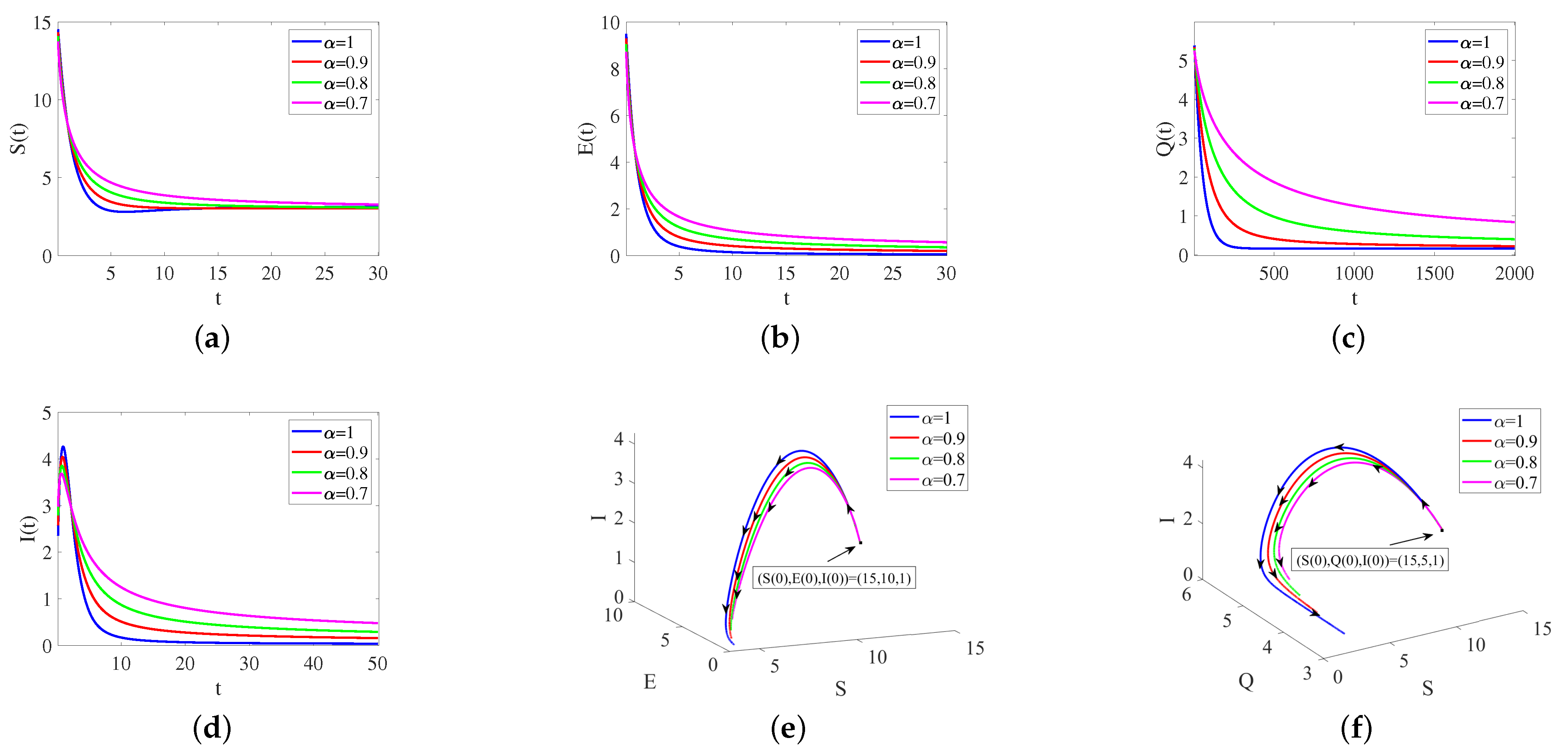
Figure 2a–f show that when R 0 = 0.8310 < 1 , according to Theorem 3, the disease-free equilibrium P 0 ( 2.4390 , 0 , 0 , 0 ) is globally asymptotically stable. In addition, the order value α change affects the system (19) convergence rate. As the value α decreases, system (19)’s memory is enhanced, resulting in a slower convergence speed, meaning it takes longer to eradicate the disease.
Remark 2.
In Figure 3a–f, system (19) simulates that when R 0 = 1.0991 > 1 , according to Theorem 4, the endemic equilibrium P * ( 3.1549 , 0.0360 , 0.1622 , 0.0375 ) is locally asymptotically stable. With the decrease in the value α, the convergence speed still has a similar pattern as the disease-free equilibrium P 0 , which means longer intervention or intensive intervention is required to eradicate the disease.
Remark 3.
In Figure 4a–c, early vaccination of the susceptible without government intervention ( κ = 0 ) can effectively reduce the number of infected among various populations. However, as the proportion of vaccinations further expands, the number of different types of the population tends to stabilize and reach a saturation state. On the other hand, without vaccination ( σ = 0 ) , with the increase in the proportion of government control, the number of susceptible populations can be effectively increased, thus reducing the number of infected people, as shown in Figure 4d–f. Therefore, the combination of vaccination and government control can better affect epidemic prevention and control.
Remark 4.
In Figure 5a, under the interference of slight white noise φ = ( 0.01 , 0.02 , 0.02 , 0.03 ) , according to Theorem 5, system (27) shows the feature of asymptotic mean-square stability at the endemic equilibrium P * . With the increase in interference intensity, system (27) will become unstable in Figure 5b–d.

6.2. Numerical Analysis with Control Strategy

Remark 5.
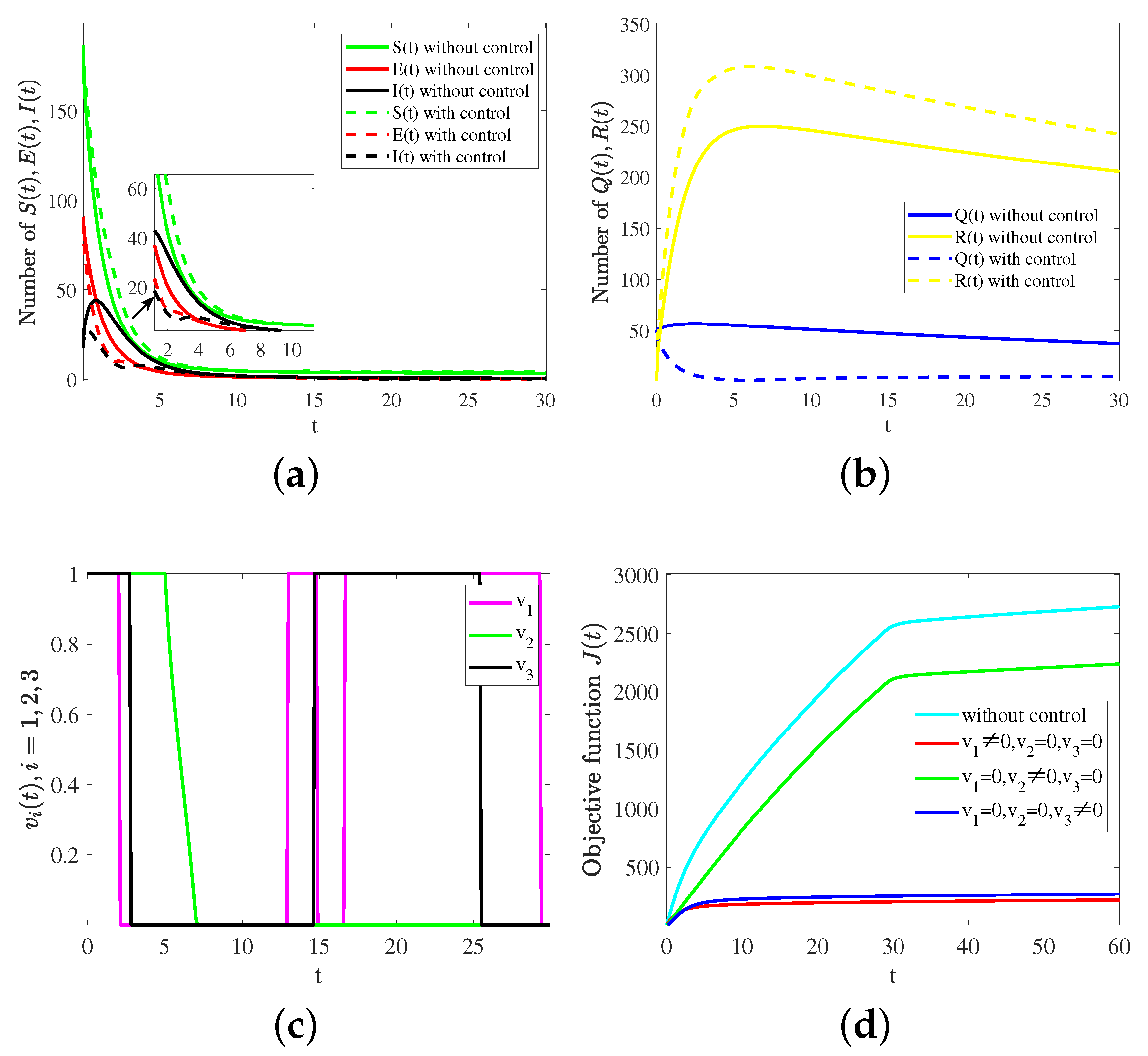
In Figure 6a,b, when α = 0.95 , compared with no control, it can be easily seen that optimal control leads to faster convergence of system (35) and corresponding changes in the steady-state value x ^ = ( S ^ , E ^ , Q ^ , I ^ , R ^ ) . Moreover, from Figure 6d, it is clear that different optimization control strategies generate different costs, so optimizing the input proportion of optimal control has the greatest economic benefit.

6.3. Sensitivity Analysis

It is very essential to discuss the sensitivity of model parameters to study the dynamics of the system. For example, the sensitivity index of the basic reproduction number R 0 to parameter Λ can be defined as [55]
Γ Λ R 0 = R 0 Λ × Λ R 0 .
In Figure 7a,b,d, κ and σ have an apparent inhibitory effect on R 0 . On the contrary, from Figure 7b–d, β has a significant promoting effect on R 0 and accelerated the spread of the epidemic. As shown in Figure 7c, by comparison, γ has little effect on R 0 .
In Figure 8, the sensitivity indices of Λ and β are positively correlated with R 0 , indicating that they strongly contribute to the spread of epidemics. Conversely, the sensitivity indices of σ and θ have a strong negative correlation with R 0 , indicating that it could effectively suppress the spread of epidemics. The sensitivity index of R 0 to relevant parameters is shown in Table 3.

7. Conclusions and Discussion

In infectious disease modeling, different incidence rates can be used for specific situations. In this paper, two kinds of saturation incidence, β S I 1 + α S and β S I 1 + b I , are introduced. In the initial stage of disease transmission, susceptible individuals have a saturation effect, and it is appropriate to use β S I 1 + α S for modeling. If the disease has developed to the stage of a large-scale epidemic, with the increase in I ( t ) , infected individuals will produce a saturation effect, which is suitable for modeling with β S I 1 + b I . Considering a pandemic such as COVID-19, a fractional SEQIR infectious disease model with isolation measures and immunization was developed using the saturated incidence of infected persons, and the threshold conditions for disease persistence and extinction were obtained. When R 0 < 1 , the disease-free equilibrium is asymptotically stable, and the disease is extinct; conversely, if R 0 > 1 , the endemic equilibrium is asymptotically stable, and the disease is persistent.
In fact, the spread of diseases will inevitably be affected by various environmental factors. In this paper, the white noise is coupled into the fractional system (19), and the corresponding stochastic infectious disease model is obtained. The stochastic stability of the positive equilibrium is discussed in the case of integer derivatives. Moreover, it is of great significance to seek optimal control strategies for major infectious diseases such as COVID-19, which seriously threaten human life, health, and social development. In this paper, an optimal control model is established by introducing control variables, and the optimal control solution of the system is obtained by using the maximum principle.
In the era of information, media publicity plays an indispensable role in disease prevention and control. The consideration of news media’s role in infectious disease modeling is a problem to be addressed in the next step. In addition, disease infection often has a latency period, and considering the impact of latency delay on the system based on the existing model is also the direction of our future work.

Author Contributions

Conceptualization, D.S.; Methodology, Q.L.; Supervision, W.Z. All authors have read and agreed to the published version of the manuscript.

Funding

This research received no external funding.

Institutional Review Board Statement

Not applicable.

Informed Consent Statement

Not applicable.

Data Availability Statement

Not applicable.

Conflicts of Interest

The authors declare no conflict of interest.

References

  1. Anderson, R.M.; May, R.M. Population biology of infectious diseases: Part I. Nature 1979, 280, 361–367. [Google Scholar] [CrossRef]
  2. Jin, Z.; Wang, J.J.; Zhang, J.Z. Analysis of an SIR model with bilinear incidence rate. Nonlinear Anal. Real World Appl. 2010, 11, 2390–2402. [Google Scholar]
  3. De-León, C.V. On the global stability of SIS, SIR and SIRS epidemic models with standard incidence. Chaos Soliton. Fract. 2011, 12, 1106–1110. [Google Scholar] [CrossRef]
  4. Hu, Z.X.; Liu, S.; Wang, H. Backward bifurcation of an epidemic model with standard incidence rate and treatment rate. Nonlinear Anal. Real World Appl. 2008, 9, 2302–2312. [Google Scholar] [CrossRef]
  5. Kar, T.K.; Mondal, P.K. Global dynamics and bifurcation in a delayed SIR epidemic model. Nonlinear Anal. Real World Appl. 2011, 12, 2058–2068. [Google Scholar] [CrossRef]
  6. Song, X.Y.; Jiang, Y.; Wei, H.M. Analysis of a saturation incidence SVEIRS epidemic model with pulse and two time delays. Appl. Math. Comput. 2009, 214, 381–390. [Google Scholar] [CrossRef]
  7. Zhang, T.; Teng, Z. Global asymptotic stability of a delayed SEIRS epidemic model with saturation incidence. Chaos Soliton. Fract. 2008, 37, 1456–1468. [Google Scholar] [CrossRef]
  8. May, R.M.; Anderson, R.M. Population biology of infectious diseases: Part II. Nature 1979, 280, 455–461. [Google Scholar] [CrossRef] [PubMed]
  9. Capasso, V.; Serio, G. A generalization of the Kermack–Mckendrick deterministic epidemic model. Math. Biosci. 1978, 42, 43–61. [Google Scholar] [CrossRef]
  10. Zhou, T.; Zhang, W.; Lu, Q. Bifurcation analysis of an SIS epidemic model with saturated incidence rate and saturated treatment function. Appl. Math. Comput. 2014, 226, 288–305. [Google Scholar] [CrossRef]
  11. Cui, X.; Xue, D.; Pan, F. Dynamic analysis and optimal control for a fractional-order delayed SIR epidemic model with saturated treatment. Eur. Phys. J. Plus. 2022, 137, 586. [Google Scholar] [CrossRef]
  12. Deng, W.H.; Li, C.P.; Lu, J.H. Stability analysis of linear fractional differential system with multiple time delays. Nonlinear Dyn. 2007, 48, 409–416. [Google Scholar] [CrossRef]
  13. Kilbas, A.A.; Srivastava, H.M.; Trujillo, J.J. Theory and Application of Fractional Differential Equations; Elsevier: Amsterdam, The Netherlands, 2006; Volume 204. [Google Scholar]
  14. Podlubny, I. Fractional Differential Equations; Academic Press: San Diego, CA, USA, 1999. [Google Scholar]
  15. Petráš, I.; Terpák, J. Fractional calculus as a simple tool for modeling and analysis of long memory process in industry. Mathematics 2019, 7, 511. [Google Scholar] [CrossRef] [Green Version]
  16. Deng, W.H. Short memory principle and a predictor-corrector approach for fractional differential equations. J. Comput. Appl. Math. 2022, 206, 174–188. [Google Scholar] [CrossRef] [Green Version]
  17. Li, R.H.; Wu, H.Q.; Gao, J.D. Exponential synchronization for variable-order fractional discontinuous complex dynamical networks with short memory via impulsive control. Neural. Netw. 2022, 148, 13–22. [Google Scholar] [CrossRef]
  18. Chinnathambi, R.; Rihan, F.A. Stability of fractional-order prey-predator system with time-delay and Monod-Haldane functional response. Nonlinear Dyn. 2018, 92, 1637–1648. [Google Scholar] [CrossRef]
  19. Qi, H.; Zhao, W.C. Stability and bifurcation control analysis of a delayed fractional-order eco-epidemiological system. Eur. Phys. J. Plus. 2022, 137, 934. [Google Scholar] [CrossRef]
  20. Rudolf, H. Applications of Fractional Calculus in Physics; World Scientific: Singapore, 2000. [Google Scholar]
  21. Khan, M.A.; Khan, Y.; Islam, S. Complex dynamics of an SEIR epidemic model with saturated incidence rate and treatment. Phys. A Stat. Mech. Appl. 2018, 493, 210–227. [Google Scholar] [CrossRef]
  22. Petras, I. Fractional-Order Nonlinear Systems: Modeling, Analysis and Simulation; Springer Science Business Media: Berlin/Heidelberg, Germany, 2011. [Google Scholar]
  23. Odibat, Z.M.; Shawagfeh, N.T. Generalized Taylor’s formula. Appl. Math. Comput. 2007, 86, 286–293. [Google Scholar] [CrossRef]
  24. Cole, K.S. Electric Conductance of Biological Systems; Cold Spring Harbor Symposia on Quantitative Biology, Cold Spring Harbor Laboratory Press: Cold Spring Harbor, NY, USA, 1933; Volume 1, pp. 107–116. [Google Scholar]
  25. Saeedian, M.; Khalighi, M.; Azimi-Tafreshi, N.; Jafari, G.R.; Ausloos, M. Memory effects on epidemic evolution: The susceptible-infected-recovered epidemic model. Phys. Rev. E 2017, 95, 022409. [Google Scholar] [CrossRef] [Green Version]
  26. Kumar, A.; Kumar, S. A study on eco-epidemiological model with fractional operators. Chaos Soliton. Fract. 2022, 156, 111697. [Google Scholar] [CrossRef]
  27. Almeida, R.; Brito da Cruz, A.M.C.; Martins, N.; Monteiro, M.T.T. An epidemiological MSEIR model described by the Caputo fractional derivative. Int. J. Dyn. Control 2018, 7, 776–784. [Google Scholar] [CrossRef] [Green Version]
  28. Paul, S.; Mahata, A.; Mukherjee, S.; Roy, B.; Salimi, M.; Ahmadian, A. Study of fractional order SEIR epidemic model and effect of vaccination on the spread of COVID-19. Int. J. Appl. Comput. Math. 2022, 8, 237. [Google Scholar] [CrossRef] [PubMed]
  29. Ameena, I.; Baleanuc, D.; Ali, H.M. An efficient algorithm for solving the fractional optimal control of SIRV epidemic model with a combination of vaccination and treatment. Chaos Soliton. Fract. 2020, 137, 109892. [Google Scholar] [CrossRef]
  30. Nabti, A.; Ghanbari, B. Global stability analysis of a fractional SVEIR epidemic model. Math. Meth. Appl. Sci. 2021, 44, 8577–8597. [Google Scholar] [CrossRef]
  31. Ahumada, M.; Ledesma-Araujo, A.; Gordillo, L.; Marín, J.F. Mutation and SARS-CoV-2 strain competition under vaccination in a modified SIR model. Chaos Soliton. Fract. 2023, 166, 112964. [Google Scholar] [CrossRef]
  32. Paul, J.N.; Mbalawata, I.S.; Mirau, S.S.; Masandawa, L. Mathematical modeling of vaccination as a control measure of stress to fight COVID-19 infections. Chaos Soliton. Fract. 2023, 166, 112920. [Google Scholar] [CrossRef]
  33. Stanislavsky, A.A. Memory effects and macroscopic manifestation of randomness. Phys. Rev. E 2000, 61, 4752. [Google Scholar] [CrossRef] [Green Version]
  34. Fan, H.; Wang, K.; Zhu, Y. Stability and asymptotic properties of the SEQIR epidemic model. Appl. Math. Lett. 2023, 141, 108604. [Google Scholar] [CrossRef]
  35. Mandal, M.; Jana, S.; Nandi, S.K.; Khatua, A.; Adak, S.; Kar, T.K. A model based study on the dynamics of COVID-19: Prediction and control. Chaos Soliton. Fract. 2020, 136, 109889. [Google Scholar] [CrossRef]
  36. Diethelm, K. Monotonicity of functions and sign changes of their caputo derivatives. Fract. Calc. Appl. Anal. 2016, 19, 561–566. [Google Scholar] [CrossRef] [Green Version]
  37. Li, H.L.; Zhang, L.; Hu, C.; Jiang, Y.L.; Teng, Z. Dynamical analysis of a fractional-order predator-prey model incorporating a prey refuge. J. Appl. Math. Comput. 2017, 54, 435–449. [Google Scholar] [CrossRef]
  38. Li, Y.; Chen, Y.Q.; Podlubny, I. Stability of fractional-order nonlinear dynamic systems: Lyapunov direct method and generalized mittag-leffer stability. Comput. Math. Appl. 2010, 59, 1810–1821. [Google Scholar] [CrossRef] [Green Version]
  39. Van den Driessche, P.; Watmough, J. Reproduction numbers and sub-threshold endemic equilibria for compartmental models of disease transmission. Math. Biosci. 2002, 180, 29–48. [Google Scholar] [CrossRef]
  40. Lahrouz, A.; Omari, L.; Kiouach, D. Global analysis ofa deterministic and stochastic non-linear SIRS epidemic model. Nonlinear Anal-Model. 2011, 16, 69–76. [Google Scholar]
  41. Majee, S.; Jana, S.; Das, D.K.; Kar, T.K. Global dynamics of a fractional-order HFMD model incorporating optimal treatment and stochastic stability. Chaos Soliton. Fract. 2022, 161, 112291. [Google Scholar] [CrossRef]
  42. Afanas’ev, V.N.; Kolmanowskii, V.B.; Nosov, V.R. Mathematical Theory of Control Systems Design; Kluwer Academic: Dordrecht, The Netherlands, 1996. [Google Scholar]
  43. Cai, L.; Li, X. A note on global stability of an SEI epidemic model with acute and chronic stages. Appl. Math. Comput. 2008, 196, 923–930. [Google Scholar] [CrossRef]
  44. Lv, Z.; Chen, D.; Feng, H.; Zhu, H.; Lv, H. Digital twins in unmanned aerial vehicles for rapid medical resource delivery in epidemics. IEEE Trans. Intell. Transp. Syst. 2021, 23, 25106–25114. [Google Scholar] [CrossRef]
  45. Luo, R.; Peng, Z.; Hu, J. On model identification based optimal control and it’s applications to multi-agent learning and control. Mathematics 2023, 11, 906. [Google Scholar] [CrossRef]
  46. Khan, M.A.; Khan, R.; Khan, Y.; Islam, S. A mathematical analysis of Pine Wilt disease with variable population size and optimal control strategies. Chaos Soliton. Fract. 2018, 108, 205–217. [Google Scholar] [CrossRef]
  47. Zhang, Z.; Wang, L.; Zheng, W.; Yin, L.; Hu, R.; Yang, B. Endoscope image mosaic based on pyramid ORB. Biomed. Signal Proces. 2022, 71, 103261. [Google Scholar] [CrossRef]
  48. Liu, Y.; Tian, J.; Hu, R.; Yang, B.; Liu, S.; Yin, L.; Zheng, W. Improved feature point pair purification algorithm based on SIFT during endoscope image stitching. Front. Neurorobot. 2022, 16, 840594. [Google Scholar] [CrossRef] [PubMed]
  49. Liu, S.; Yang, B.; Wang, Y.; Tian, J.; Yin, L.; Zheng, W. 2D/3D multimode medical image registration based on normalized cross-correlation. Appl. Sci. 2022, 12, 2828. [Google Scholar] [CrossRef]
  50. Göllmann, L.; Kern, D.; Maurer, H. Optimal control problems with delays in state and control variables subject to mixed control-state constraints. Optim. Control Appl. Meth. 2009, 30, 341–365. [Google Scholar] [CrossRef]
  51. Fleming, W.H.; Rishel, R.W. Deterministic and Stochastic Optimal Control; Springer: New York, NY, USA; Berlin/Heidelberg, Germany, 1975. [Google Scholar]
  52. Shi, R.; Lu, T. Dynamic analysis and optimal control of a fractional order model for hand-foot-mouth disease. J. Appl. Math. Comput. 2020, 64, 565–590. [Google Scholar] [CrossRef]
  53. Lukes, D.L. Differential Equations: Classical to Controlled; Mathematics in Science and Engineering; Academic Press: New York, NY, USA, 1982. [Google Scholar]
  54. Baskonus, H.M.; Bulut, H. On the numerical solutions of some fractional ordinary differential equations by fractional Adams-Bashforth-Moulton method. Open Math. 2015, 13, 547–556. [Google Scholar] [CrossRef]
  55. Das, D.K.; Kar, T.K. Global dynamics of a tuberculosis model with sensitivity of the smear microscopy. Chaos Soliton. Fract. 2021, 146, 110879. [Google Scholar] [CrossRef]
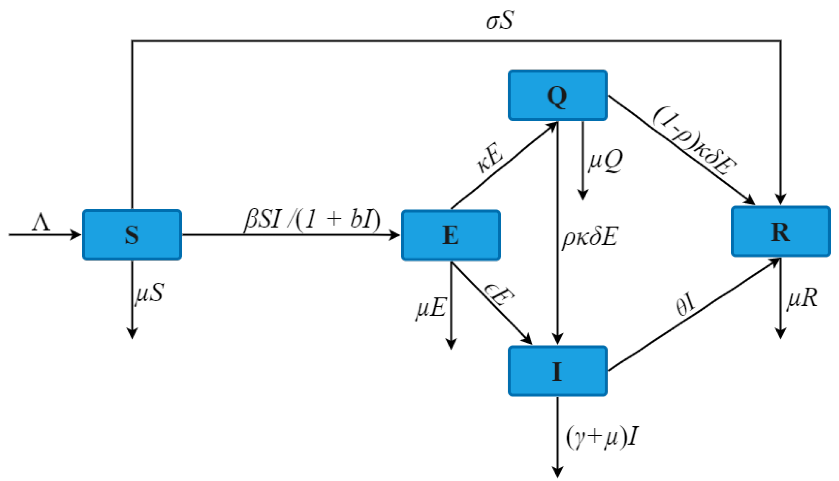
Figure 1. Basic framework of epidemic transmission.
Fractalfract 07 00533 g001
Figure 2. In (af), the system (19) exhibits locally asymptotic stability at the disease-free equilibrium P 0 and the time when the fractional order α changes affect the stability.
Fractalfract 07 00533 g002
Figure 3. In (af), the system (19) exhibits locally asymptotic stability at the endemic equilibrium P * and the time when the fractional order α changes affect the stability.
Fractalfract 07 00533 g003
Figure 4. In (ac), the impact of increasing immunization rates σ on S ( t ) , E ( t ) , and I ( t ) ; In (df), the effect of increasing proportion of government control κ on S ( t ) , E ( t ) , and I ( t ) .
Fractalfract 07 00533 g004
Figure 5. Dynamic behavior of system (27) in a random environment. White noise: (a) φ = ( 0.01 , 0.02 , 0.02 , 0.03 ) , (b) φ = ( 0.1 , 0.3 , 0.2 , 0.3 ) , (c) φ = ( 0.2 , 0.5 , 0.5 , 0.6 ) , (d) φ = ( 0.6 , 0.8 , 1.2 , 1 ) .
Fractalfract 07 00533 g005
Figure 6. With optimal control, the stability of the system (35) near the endemic equilibrium x ^ (a,b), and the corresponding optimal control solution v i ( t ) , i = 1 , 2 , 3 (c) and objective function values J ( t ) (d).
Fractalfract 07 00533 g006
Figure 7. In (ad), the correlation of parameters κ , σ , β , γ to R 0 is verified. Fixed parameter value: κ = 0.6 , σ = 0.6 , γ = 0.1 , β = 0.4 .
Fractalfract 07 00533 g007
Figure 8. Correlation between parameters and sensitivity index.
Fractalfract 07 00533 g008
Table 2. Other parameter values for specific examples in numerical simulation.
Parameters Λ σ κ α
Remark 120.80.6[1 0.9 0.8 0.7]
Remark 220.60.6[1 0.9 0.8 0.7]
Remark 32[0 0.3 0.6 0.9][0 0.3 0.6 0.9]0.95
Remark 4100.80.61
Remark 520.60.60.95
Table 3. Value of sensitivity index of R 0 -related parameters.
Parameters Λ β σ μ κ
Sensitivity index value+0.7839+0.8276−0.6674−0.1750−0.1707
Parameters ϵ θ γ ρ δ
Sensitivity index value+0.1224−0.5220−0.06522+0.1363+0.1664
Disclaimer/Publisher’s Note: The statements, opinions and data contained in all publications are solely those of the individual author(s) and contributor(s) and not of MDPI and/or the editor(s). MDPI and/or the editor(s) disclaim responsibility for any injury to people or property resulting from any ideas, methods, instructions or products referred to in the content.