Applications to Nonlinear Fractional Differential Equations via Common Fixed Point on ℂ^★-Algebra-Valued Bipolar Metric Spaces

Abstract

In the present paper, we prove common fixed point theorems under different contractive mappings on ${\mathbb{C}}^{★}$-algebra-valued bipolar metric spaces. The results generalize and expand some well-known results from the literature. Examples and applications are given to strengthen our conclusion. Additionally, as an application of our results, we show that some classes of the nonlinear fractional differential equations with the boundary conditions have a unique common solution.

1. Introduction to Fractional Calculus

Mutlu and Gürdal [1] initiated the new concept “bipolar metric space” in 2016, as follows.

Definition 1.

[1] Let ξ and Υ be two nonempty sets and $\partial :\xi \times \mathit{{\rm Y}}\to {\mathbb{R}}^{+}$ be a function, such that

(1) 

$\mathit{\partial }(𝚤,𝚥)=0\iff 𝚤=𝚥$, for all $(𝚤,𝚥)\in \xi \times {\rm Y}$

(2) 

$\partial (𝚤,𝚥)=\partial \left(𝚥,𝚤\right)$, for all $(𝚤,𝚥)\in \xi \cap {\rm Y}$

(3) 

$\partial (𝚤,𝚥)\le \partial (𝚤,\mathfrak{z})+\partial ({𝚤}_1,\mathfrak{z})+\partial ({𝚤}_1,𝚥)$, for all $𝚤,{𝚤}_1\in \xi$ and $\mathfrak{z},𝚥\in {\rm Y}$.

The pair $(\xi ,{\rm Y},\partial )$ is said to be a bipolar metric space.

Numerous researchers have provided fixed point results in bipolar metric spaces (see [2,3,4,5,6,7,8,9]). Recently, Ma et al. [10] presented their work on the extension of the Banach contraction principle for ${\mathbb{C}}^{★}$-algebra-valued metric spaces. Later, Batul and Kamran [11] introduced the notion of a ${\mathbb{C}}^{★}$-valued contractive type mapping and established a fixed point result in this setting. Gunaseelan et al. [12] initiated ${\mathtt{C}}^{★}$-algebra-valued bipolar metric spaces and established some coupled fixed point results. Gunaseelan et al. [13] proved fixed point theorems on $C^{★}$-algebra-valued bipolar metric spaces (in short, $C^{★}$-AVBMS) with an application. Recently, Rajagopalan et al. [14] proved fixed point theorems on covariant and contravariant maps.

We now recollect some basic definitions, notations, and results. The details on ${\mathbb{C}}^{★}$-algebra are available in [15,16,17,18].

An algebra $\Lambda$, together with a conjugate linear involution map $\mathfrak{o}⟼{\mathfrak{o}}^{★}$, is called a ★-algebra if ${\left(\mathfrak{o}\mathfrak{n}\right)}^{★}={\mathfrak{n}}^{★}{\mathfrak{o}}^{★}$ and ${\left({\mathfrak{o}}^{★}\right)}^{★}=\mathfrak{o}$ for all $\mathfrak{a},\mathfrak{b}\in \Lambda$. Moreover, the pair $(\Lambda ,★)$ is called a unital ★-algebra if $\Lambda$ contains the identity element $1_{\Lambda }$. By a Banach ★-algebra we mean a complete normed unital ★-algebra $(\Lambda ,★)$ such that the norm on $\Lambda$ is submultiplicative and satisfies $\parallel {\mathfrak{o}}^{★}\parallel =\parallel \mathfrak{o}\parallel$ for all $\mathfrak{o}\in \Lambda$. Further, if for all $\mathfrak{o}\in \Lambda$, we have $\parallel {\mathfrak{o}}^{★}\mathfrak{o}\parallel =\parallel \mathfrak{o}{\parallel }^2$ in a Banach ★-algebra $(\Lambda ,★)$, then $\Lambda$ is known as a ${\mathbb{C}}^{★}$-algebra. A positive element of $\Lambda$ is an element $\mathfrak{o}\in \Lambda$ such that $\mathfrak{o}={\mathfrak{o}}^{★}$ and its spectrum $\left(\mathfrak{o}\right)\subset {\mathbb{R}}_{+}$, where $\left(\mathfrak{o}\right)$ = $\{\in \mathbb{R}:1_{\Lambda }-\mathfrak{o}\mathrm{is}\mathrm{noninvertible}\}$. The set of all positive elements is denoted by ${\Lambda }_{+}$. Such elements allow us to define a partial ordering ⪰ on the elements of $\Lambda$. That is,

$$\begin{array}{c}\hfill \mathfrak{n}⪰\mathfrak{o}\mathrm{if}\mathrm{and}\mathrm{only}\mathrm{if}\mathfrak{n}-\mathfrak{o}\in {\Lambda }_{+}.\end{array}$$

If $\mathfrak{o}\in \Lambda$ is positive, then we write $\mathfrak{o}⪰0_{\Lambda }$, where $0_{\Lambda }$ is the zero element of $\Lambda$. Each positive element $\mathfrak{o}$ of a ${\mathbb{C}}^{★}$-algebra $\Lambda$ has a unique positive square root. From now on, by $\Lambda$ we mean a unital ${\mathbb{C}}^{★}$-algebra with the identity element $1_{\Lambda }$. Further, ${\Lambda }_{+}$ = $\{\mathfrak{o}\in \Lambda :\mathfrak{o}⪰0_{\Lambda }\}$ and ${\left({\mathfrak{o}}^{★}\mathfrak{o}\right)}^{1/2}$ =$\left|\mathfrak{o}\right|$. In this paper, we prove common fixed point theorems under different contractive mappings on ${\mathtt{C}}^{★}$-algebra-valued bipolar metric spaces.

2. Preliminaries

Gunaseelan et al. [12] initiated the concept “bipolar metric space” in the notion of “${\mathbb{C}}^{★}$-algebra” in 2022, as follows.

Definition 2.

Let Λ be a ${\mathbb{C}}^{*}$-algebra and ξ, Υ be two nonvoid sets. A mapping $\partial :\xi \times {\rm Y}\to {\Lambda }_{+}$ is a function such that

(a) 

$\partial (𝚤,𝚥)=0$ if and only if $𝚤=𝚥$, for all $(𝚤,𝚥)\in \xi \times {\rm Y}$

(b) 

$\partial (𝚤,𝚥)=\partial (𝚥,𝚤)$, for all $(𝚤,𝚥)\in \xi \cap {\rm Y}$

(c) 

$\partial (𝚤,𝚥)\le \partial (𝚤,\gamma )+\partial ({𝚤}_1,\gamma )+\partial ({𝚤}_1,𝚥)$, for all $𝚤,{𝚤}_1\in \xi$ and $\gamma ,𝚥\in {\rm Y}$.

The 4-tuple $(\xi ,{\rm Y},\Lambda ,\partial )$ is called a $C^{★}$-AVBMS.

Next, we recall a lemma and some definitions:

Lemma 1

([16,18]). Assume that Λ is a unital ${\mathbb{C}}^{★}$-algebra with a unit $\mathfrak{T}$.

(A1) 

For any $𝚤\in {\Lambda }_{+}$, $𝚤⪯\mathfrak{T}$ if and only if $\left|\right|𝚤\left|\right|\le 1$.

(A2) 

If $\left|\right|\mathfrak{o}\left|\right|<\frac{1}{2}$ for all $\mathfrak{o}\in {\Lambda }_{+}$, then $(\mathfrak{T}-\mathfrak{o})$ is invertible and ${\left|\right|\mathfrak{o}(\mathfrak{T}-a)}^{-1}\left|\right|<1$.

(A3) 

Suppose that $\mathfrak{o},\mathfrak{n}\in \Lambda$ with $\mathfrak{o}\mathfrak{n}⪰0_{\Lambda }$ and $\mathfrak{o}\mathfrak{n}=\mathfrak{n}\mathfrak{o}$. Then, $\mathfrak{o}\mathfrak{n}⪰0_{\Lambda }$.

(A4) 

By ${\Lambda }^{\prime }$, we denote the set $\{\mathfrak{o}\in \Lambda :\mathfrak{o}\mathfrak{n}=\mathfrak{n}\mathfrak{o},\forall \mathfrak{n}\in \Lambda \}$. Letting $\mathfrak{o}\in {\Lambda }^{\prime }$, if $\mathfrak{n},\mathfrak{c}\in \Lambda$ with $\mathfrak{n}⪰\mathfrak{c}⪰0_{\Lambda }$, and $\mathfrak{T}-\mathfrak{o}\in {\Lambda }_{+}^{\prime }$ is an invertible operator, then

$$\begin{array}{c}\hfill {(\mathfrak{T}-\mathfrak{o})}^{-1}\mathfrak{n}⪰{(\mathfrak{T}-\mathfrak{o})}^{-1}\mathfrak{c}.\end{array}$$

Definition 3.

Let $({\xi }_1,{{\rm Y}}_1,\Lambda ,\partial )$ and $({\xi }_2,{{\rm Y}}_2,\Lambda ,\partial )$ be pairs of sets and a map $\mathcal{W}:{\xi }_1\cup {{\rm Y}}_1\to {\xi }_2\cup {{\rm Y}}_2$.

(B1) 

If $\mathcal{W}\left({\xi }_1\right)\subseteq {\xi }_2$ and $\mathcal{W}\left({{\rm Y}}_1\right)\subseteq {{\rm Y}}_2$, then $\mathcal{W}$ is called a covariant map, or a map from $({\xi }_1,{{\rm Y}}_1,\Lambda ,{\partial }_1)$ to $({\xi }_2,{{\rm Y}}_2,\Lambda ,{\partial }_2)$, and this is written as $\mathcal{W}:({\xi }_1,{{\rm Y}}_1,\Lambda ,{\partial }_1)\rightrightarrows ({\xi }_2,{{\rm Y}}_2,\Lambda ,{\partial }_2)$.

(B2) 

If $\mathcal{W}\left({\xi }_1\right)\subseteq {{\rm Y}}_2$ and $\mathcal{W}\left({{\rm Y}}_1\right)\subseteq {\xi }_2$, then $\mathcal{W}$ is called a contravariant map from $({\xi }_1,{{\rm Y}}_1,\Lambda ,{\partial }_1)to({\xi }_2,{{\rm Y}}_2,\Lambda ,{\partial }_2)$, and this is denoted as $\mathcal{W}:({\xi }_1,{{\rm Y}}_1,\Lambda ,{\partial }_1)\leftrightarrows ({\xi }_2,{{\rm Y}}_2,\Lambda ,{\partial }_2)$.

Definition 4.

Let $(\xi ,{\rm Y},\Lambda ,\partial )$ be a $C^{★}$-AVBMS.

(C1) 

A point $𝚤\in \xi \cup {\rm Y}$ is called a left point if $𝚤\in \xi$, a right point if $𝚤\in {\rm Y}$, and a central point if both hold. Similarly, a sequence $\left\{{𝚤}_{\delta }\right\}$ on the set ξ and a sequence $\left\{{𝚥}_n\right\}$ on the set Υ are called left and right sequences with respect to (w.r.t) Λ, respectively.

(C2) 

A sequence $\left\{{𝚤}_{\delta }\right\}$ converges to a point j w.r.t Λ iff $\left\{{𝚤}_{\delta }\right\}$ is a left sequence, j is a right point, and $\underset{\delta \to \infty }{lim}\partial ({𝚤}_{\delta },𝚥)=0$ or $\left\{{𝚤}_{\delta }\right\}$ is a right sequence, j is a left point, and $\underset{\delta \to \infty }{lim}\partial (𝚥,{𝚤}_{\delta })=0$.

(C3) 

A bisequence $(\left\{{𝚤}_n\right\},\left\{{𝚥}_n\right\})$ is a sequence on the set $\xi \times {\rm Y}$. If the sequences $\left\{{𝚤}_n\right\}$ and $\left\{{𝚥}_n\right\}$ are convergent w.r.t Λ, then the bisequence $(\left\{{𝚤}_n\right\},\left\{{𝚥}_n\right\})$ is called a convergent w.r.t Λ. $(\left\{{𝚤}_n\right\},\left\{{𝚥}_n\right\})$ is a Cauchy bisequence w.r.t Λ if $\underset{\delta ,\mathfrak{m}\to \infty }{lim}\partial ({𝚤}_{\delta },{𝚥}_{\mathfrak{m}})=0$; hence, it is biconvergent w.r.t Λ.

(C4) 

$(\xi ,{\rm Y},\Lambda ,\partial )$ is complete, if every Cauchy bisequence is convergent w.r.t Λ in $\xi \times {\rm Y}$.

Definition 5.

Suppose that ξ and Υ are ${\mathbb{C}}^{★}$-algebras. A mapping $\psi :\xi \to {\rm Y}$ is said to be a ${\mathbb{C}}^{★}$-homomorphism if

(U1) 

$\psi (\mathfrak{o}𝚤+\mathfrak{n}𝚥)=\mathfrak{o}\psi \left(𝚤\right)+\mathfrak{n}\psi \left(𝚥\right)$ for all $\mathfrak{o},\mathfrak{n}\in \mathbb{C}$ and $𝚤,𝚥\in \xi$;

(U2) 

$\psi \left(𝚤𝚥\right)=\psi \left(𝚤\right)\psi \left(𝚥\right)$ for all $𝚤,𝚥\in \xi$;

(U3) 

$\psi \left({𝚤}^{★}\right)=\psi {\left(𝚤\right)}^{★}$ for all $𝚤\in \xi$;

(U4) 

ψ maps the unit in ξ to the unit in Υ.

Definition 6.

Let ${\Psi }_{\Lambda }$ be the set of positive functions ${\psi }_{\Lambda }:{\Lambda }_{+}\to {\Lambda }_{+}$ such that

(R1) 

${\psi }_{\Lambda }\left(\mathfrak{o}\right)$ is continuous and nondecreasing;

(R2) 

${\psi }_{\Lambda }\left(\mathfrak{o}\right)=0$ iff $\mathfrak{o}=0$;

(R3) 

${\sum }_{\delta =1}^{\infty }{\psi }_{\Lambda }^{\delta }\left(\mathfrak{o}\right)<\infty$, $\underset{\delta \to \infty }{lim}{\psi }_{\Lambda }^{\delta }\left(\mathfrak{o}\right)=0$ for each $\mathfrak{o}\succ 0$, where ${\psi }_{\Lambda }^{\delta }$ is the δth iterate of ${\psi }_{\Lambda }$.

Definition 7.

Letting $(\xi ,{\rm Y},\Lambda ,\partial )$ be a $C^{★}$-AVBMS and ${\alpha }_{\Lambda }:\xi \times {\rm Y}\to {\Lambda }_{+}$ be a function, we say that the covariant map $\mathcal{W}$ is ${\alpha }_{\Lambda }$-covariant admissible if $𝚤\in \xi$, $𝚥\in {\rm Y}$, ${\alpha }_{\Lambda }(𝚤,𝚥)⪰{\mathfrak{T}}_{\Lambda }$ implies that ${\alpha }_{\Lambda }(\mathcal{W}𝚤,\mathcal{W}𝚥)⪰{\mathfrak{T}}_{\Lambda }$, where ${\mathfrak{T}}_{\Lambda }$ is the unit of Λ.

Definition 8.

Letting $(\xi ,{\rm Y},\Lambda ,\partial )$ be a $C^{★}$-AVBMS and $\mathcal{W}:(\xi ,{\rm Y},\Lambda ,\partial )\rightrightarrows (\xi ,{\rm Y},\Lambda ,\partial )$ be a covariant mapping, we say that the covariant map $\mathcal{W}$ is ${\alpha }_{\Lambda }$-${\psi }_{\Lambda }$-covariant contractive mapping if two functions ${\alpha }_{\Lambda }:\xi \times {\rm Y}\to {\Lambda }_{+}$ and ${\psi }_{\Lambda }\in {\Psi }_{\Lambda }$ exist, such that

$$\begin{array}{c}\hfill {\alpha }_{\Lambda }(𝚤,𝚥){\partial }_{\Lambda }(\mathcal{W}𝚤,\mathcal{W}𝚥)⪯{\psi }_{\Lambda }\left({\partial }_{\Lambda }(𝚤,𝚥)\right),\end{array}$$

for all $𝚤\in \xi$, $𝚥\in {\rm Y}$.

In this paper, we prove common fixed point theorems under different contractive mappings on ${\mathtt{C}}^{★}$-algebra-valued bipolar metric spaces.

3. Main Results

In this section, we prove common fixed point theorems on two covariant mappings.

Theorem 1.

Let $(\xi ,{\rm Y},\Lambda ,\partial )$ be a complete $C^{★}$-AVBMS. Suppose $\mathcal{W},\mathcal{V}:(\xi ,{\rm Y},\Lambda ,\partial )\rightrightarrows (\xi ,{\rm Y},\Lambda ,\partial )$ are two covariant mappings, such that

$$\begin{array}{c}\hfill \partial (\mathcal{W}𝚤,\mathcal{W}𝚥)⪯{\rho }^{★}\partial (\mathcal{V}𝚤,\mathcal{V}𝚥)\rho \mathrm{for}\mathrm{all}𝚤\in \xi ,𝚥\in {\rm Y},\end{array}$$

where $\rho \in \Lambda$, ${\left|\right|\rho \left|\right|}^2<1$, $\mathcal{W}\left(\xi \right)\subseteq \mathcal{V}\left(\xi \right)$ and $\mathcal{W}\left({\rm Y}\right)\subseteq \mathcal{V}\left({\rm Y}\right)$. Then, the functions $\mathcal{W},\mathcal{V}:\xi \cup {\rm Y}\to \xi \cup {\rm Y}$ have a unique common fixed point.

Proof. 

If $\Lambda =\left\{0_{\Lambda }\right\}$, then there is nothing to demonstrate. Suppose that $\Lambda \ne \left\{0_{\Lambda }\right\}$. Let ${𝚤}_0\in \xi$ and ${𝚥}_0\in {\rm Y}$ and choose ${𝚤}_1\in \xi$ and ${𝚥}_1\in {\rm Y}$ such that $\mathcal{W}{𝚤}_0=\mathcal{V}{𝚤}_1$ and $\mathcal{W}{𝚥}_0=\mathcal{V}{𝚥}_1$. For each $\delta \in \mathbb{N}$, define $\mathcal{W}\left({𝚤}_{2\delta -1}\right)=\mathcal{V}{𝚤}_{2\delta }$ and $\mathcal{W}\left({𝚥}_{2\delta -1}\right)=\mathcal{V}{𝚥}_{2\delta }$. Then, $(\left\{\mathcal{W}{𝚤}_{\delta }\right\},\left\{\mathcal{W}{𝚥}_{\delta }\right\})$ and $(\left\{\mathcal{V}{𝚤}_{\delta }\right\},\left\{\mathcal{V}{𝚥}_{\delta }\right\})$ are bisequences on $(\xi ,{\rm Y},\Lambda ,\partial )$. Let $\mathcal{M}:=\partial (\mathcal{V}{𝚤}_0,\mathcal{V}{𝚥}_0)+\partial (\mathcal{V}{𝚤}_0,\mathcal{V}{𝚥}_1)$. Then, for each $\delta ,\varsigma \in {\mathbb{Z}}^{+}$,

$$\begin{array}{cc}\hfill \partial (\mathcal{V}{𝚤}_{2\delta +1},\mathcal{V}{𝚥}_{2\delta +2})=& \partial (\mathcal{W}{𝚤}_{2\delta },\mathcal{W}{𝚥}_{2\delta +1})\hfill \\ \hfill & ⪯{\rho }^{★}\partial (\mathcal{V}{𝚤}_{2\delta },\mathcal{V}{𝚥}_{2\delta +1})\rho \hfill \\ \hfill & ={\rho }^{★}\partial (\mathcal{W}{𝚤}_{2\delta -1},\mathcal{W}{𝚥}_{2\delta })\rho \hfill \\ \hfill & ⪯{\left({\rho }^{★}\right)}^2\partial (\mathcal{V}{𝚤}_{2\delta -1},\mathcal{V}{𝚥}_{2\delta }){\rho }^2\hfill \\ \hfill & ⋮\hfill \\ \hfill & ⪯{\left({\rho }^{★}\right)}^{2\delta +1}\partial (\mathcal{V}{𝚤}_{\mathfrak{0}},\mathcal{V}{𝚥}_1){\rho }^{2\delta +1},\hfill \end{array}$$

$$\begin{array}{cc}\hfill \partial (\mathcal{V}{𝚤}_{2\delta +1},\mathcal{V}{𝚥}_{2\delta +1})=& \partial (\mathcal{W}{𝚤}_{2\delta },\mathcal{W}{𝚥}_{2\delta })\hfill \\ \hfill & ⪯{\rho }^{★}\partial (\mathcal{V}{𝚤}_{2\delta },\mathcal{V}{𝚥}_{2\delta })\rho \hfill \\ \hfill & ={\rho }^{★}\partial (\mathcal{W}{𝚤}_{2\delta -1},\mathcal{W}{𝚥}_{2\delta -1})\rho \hfill \\ \hfill & ⪯{\left({\rho }^{★}\right)}^2\partial (\mathcal{V}{𝚤}_{2\delta -1},\mathcal{V}{𝚥}_{2\delta -1}){\rho }^2\hfill \\ \hfill & ⋮\hfill \\ \hfill & ⪯{\left({\rho }^{★}\right)}^{2\delta +1}\partial (\mathcal{V}{𝚤}_{\mathfrak{0}},\mathcal{V}{𝚥}_{\mathfrak{0}}){\rho }^{2\delta +1}.\hfill \end{array}$$

$$\begin{array}{cc}\hfill \partial (\mathcal{V}{𝚤}_{\delta +\varsigma },\mathcal{V}{𝚥}_{\delta })& ⪯\partial (\mathcal{V}{𝚤}_{\delta +\varsigma },\mathcal{V}{𝚥}_{\delta +1})+\partial (\mathcal{V}{𝚤}_{\delta },\mathcal{V}{𝚥}_{\delta +1})+\partial (\mathcal{V}{𝚤}_{\delta },\mathcal{V}{𝚥}_{\delta })\hfill \\ \hfill & ⪯\partial (\mathcal{V}{𝚤}_{\delta +\varsigma },\mathcal{V}{𝚥}_{\delta +1})+{\left({\rho }^{★}\right)}^{\delta }\mathcal{M}{\rho }^{\delta }\hfill \\ \hfill & ⪯\partial (\mathcal{V}{𝚤}_{\delta +\varsigma },\mathcal{V}{𝚥}_{\delta +2})+\partial (\mathcal{V}{𝚤}_{\delta +1},\mathcal{V}{𝚥}_{\delta +2})+\partial (\mathcal{V}{𝚤}_{\delta +1},\mathcal{V}{𝚥}_{\delta +1})\hfill \\ \hfill & +{\left({\rho }^{★}\right)}^{\delta }\mathcal{M}{\rho }^{\delta }\hfill \\ \hfill & ⪯\partial (\mathcal{V}{𝚤}_{\delta +\varsigma },\mathcal{V}{𝚥}_{\delta +2})+{\left({\rho }^{★}\right)}^{\delta +1}\mathcal{M}{\rho }^{\delta +1}+{\left({\rho }^{★}\right)}^{\delta }\mathcal{M}{\rho }^{\delta }\hfill \\ \hfill & ⋮\hfill \\ \hfill & ⪯\partial (\mathcal{V}{𝚤}_{\delta +\varsigma },\mathcal{V}{𝚥}_{\delta +\varsigma })+{\left({\rho }^{★}\right)}^{\delta +\varsigma -1}\mathcal{M}{\rho }^{\delta +\varsigma -1}\hfill \\ \hfill & +\cdots +{\left({\rho }^{★}\right)}^{\delta +1}\mathcal{M}{\rho }^{\delta +1}+{\left({\rho }^{★}\right)}^{\delta }\mathcal{M}{\rho }^{\delta }\hfill \\ \hfill & ⪯{\left({\rho }^{★}\right)}^{\delta +\varsigma }\mathcal{M}{\rho }^{\delta +\varsigma }+{\left({\rho }^{★}\right)}^{\delta +\varsigma -1}\mathcal{M}{\rho }^{\delta +\varsigma -1}+\cdots +{\left({\rho }^{★}\right)}^{\delta +1}\mathcal{M}{\rho }^{\delta +1}\hfill \\ \hfill & +{\left({\rho }^{★}\right)}^{\delta }\mathcal{M}{\rho }^{\delta }\hfill \\ \hfill & =\sum _{\mathfrak{k}=\delta }^{\delta +\varsigma }{\left({\rho }^{★}\right)}^{\mathfrak{k}}\mathcal{M}{\rho }^{\mathfrak{k}}\hfill \\ \hfill & =\sum _{\mathfrak{k}=\delta }^{\delta +\varsigma }{\left({\rho }^{★}\right)}^{\mathfrak{k}}{\mathcal{M}}^{\frac{1}{2}}{\mathcal{M}}^{\frac{1}{2}}{\rho }^{\mathfrak{k}}\hfill \\ \hfill & =\sum _{\mathfrak{k}=\delta }^{\delta +\varsigma }{\left({\mathcal{M}}^{\frac{1}{2}}{\rho }^{\mathfrak{k}}\right)}^{★}{\mathcal{M}}^{\frac{1}{2}}{\rho }^{\mathfrak{k}}\hfill \\ \hfill & =\sum _{\mathfrak{k}=\delta }^{\delta +\varsigma }{\left|{\mathcal{M}}^{\frac{1}{2}}{\rho }^{\mathfrak{k}}\right|}^2\hfill \\ \hfill & ⪯\sum _{\mathfrak{k}=\delta }^{\delta +\varsigma }\left|\right|{\mathcal{M}}^{\frac{1}{2}}{\rho }^{\mathfrak{k}}{\left|\right|}^2{1}_{\Lambda }\hfill \\ \hfill & ⪯\sum _{\mathfrak{k}=\delta }^{\delta +\varsigma }\left|\right|\mathcal{M}\left|\right|\left|\right|{\rho }^{\mathfrak{k}}{\left|\right|}^2{1}_{\Lambda }\hfill \end{array}$$

$$\begin{array}{cc}\hfill \partial (\mathcal{V}{𝚤}_{\delta +\varsigma },\mathcal{V}{𝚥}_{\delta })& ⪯\left|\right|\mathcal{M}\left|\right|\sum _{\mathfrak{k}=\delta }^{\delta +\varsigma }\left|\right|{\rho }^2{\left|\right|}^{\mathfrak{k}}{1}_{\Lambda }\hfill \\ \hfill & \to 0_{\Lambda }\mathrm{as}\delta ,\varsigma \to \infty .\hfill \end{array}$$

Similarly, we can prove

$$\begin{array}{cc}\hfill \partial (\mathcal{V}{𝚥}_{\delta },\mathcal{V}{𝚤}_{\delta +\varsigma })& \to 0_{\Lambda }\mathrm{as}\delta ,\varsigma \to \infty .\hfill \end{array}$$

Consequently,

$$\begin{array}{cc}\hfill \partial (\mathcal{W}{𝚤}_{\delta +\varsigma },\mathcal{W}{𝚥}_{\delta })& \to 0_{\Lambda }\mathrm{as}\delta ,\varsigma \to \infty .\hfill \end{array}$$

Therefore, $(\left\{\mathcal{V}{𝚤}_{\delta }\right\},\left\{\mathcal{V}{𝚥}_{\delta }\right\})$ and $(\left\{\mathcal{W}{𝚤}_{\delta }\right\},\left\{\mathcal{W}{𝚥}_{\delta }\right\})$ are Cauchy bisequences in $(\xi ,{\rm Y},\Lambda ,\partial )$ w.r.t Λ. By completeness of $(\xi ,{\rm Y},\Lambda ,\partial )$, it follows that $\mathcal{V}{𝚤}_{\delta }\to \mathfrak{u}$ and $\mathcal{V}{𝚥}_{\delta }\to \mathfrak{u}$, where $\mathfrak{u}\in \xi \cap {\rm Y}$. Consequently, $\mathcal{W}{𝚤}_{\delta }\to \mathfrak{u}$ and $\mathcal{W}{𝚥}_{\delta }\to \mathfrak{u}$, where $\mathfrak{u}\in \xi \cap {\rm Y}$. Now,

$$\begin{array}{cc}\hfill \partial (\mathcal{V}\mathfrak{u},\mathfrak{u})& ⪯\partial (\mathcal{V}\mathfrak{u},\mathcal{V}{𝚥}_{\delta +1})+\partial (\mathcal{V}{𝚤}_{\delta +1},\mathcal{V}{𝚥}_{\delta +1})+\partial (\mathcal{V}{𝚤}_{\delta +1},\mathfrak{u}).\hfill \end{array}$$

As $\delta \to \infty$,

$$\begin{array}{c}\hfill \partial (\mathcal{V}\mathfrak{u},\mathfrak{u})=0_{\Lambda }.\end{array}$$

Therefore, $\mathcal{V}\left(\mathfrak{u}\right)=\mathfrak{u}$.

$$\begin{array}{cc}\hfill \partial (\mathcal{W}\mathfrak{u},\mathfrak{u})& ⪯\partial (\mathcal{W}\mathfrak{u},\mathcal{W}{𝚥}_{\delta +1})+\partial (\mathcal{W}{𝚤}_{\delta +1},\mathcal{W}{𝚥}_{\delta +1})+\partial (\mathcal{W}{𝚤}_{\delta +1},\mathfrak{u}).\hfill \end{array}$$

As $\delta \to \infty$,

$$\begin{array}{c}\hfill \partial (\mathcal{W}\mathfrak{u},\mathfrak{u})=0_{\Lambda }.\end{array}$$

Therefore, $\mathcal{W}\left(\mathfrak{u}\right)=\mathfrak{u}$. Hence, $\mathfrak{u}$ is common fixed point of $\mathcal{W}$ and $\mathcal{V}$. Let $\mathfrak{v}\in \xi \cup {\rm Y}$ be a another common fixed point of ξ and Υ, such that $\mathcal{V}\mathfrak{v}=\mathcal{W}\mathfrak{v}=\mathfrak{v}$. Then,

$$\begin{array}{c}\hfill 0_{\Lambda }⪯\partial (\mathfrak{u},\mathfrak{v})=\partial (\mathcal{W}\mathfrak{u},\mathcal{W}\mathfrak{v})⪯{\rho }^{*}\partial (\mathcal{V}\mathfrak{u},\mathcal{V}\mathfrak{v})\rho ={\rho }^{*}\partial (\mathfrak{u},\mathfrak{v})\rho .\end{array}$$

Using the norm of Λ, we have

$$\begin{array}{c}\hfill 0\le \parallel \partial (\mathfrak{u},\mathfrak{v})\parallel \le \parallel {\rho }^{*}\partial (\mathfrak{u},\mathfrak{v})\rho \parallel \le \parallel {\rho }^{*}\parallel \parallel \partial (\mathfrak{u},\mathfrak{v})\parallel \parallel \rho \parallel =\parallel \rho {\parallel }^2\parallel \partial (\mathfrak{u},\mathfrak{v})\parallel .\end{array}$$

The above inequality holds only when $\partial (\mathfrak{u},\mathfrak{v})=0_{\Lambda }$. Hence, $\mathfrak{u}=\mathfrak{v}$. □

Theorem 2.

Let $(\xi ,{\rm Y},\Lambda ,\partial )$ be a complete $C^{★}$-AVBMS. Suppose $\mathcal{W},\mathcal{V}:(\xi ,{\rm Y},\Lambda ,\partial )\leftrightarrows (\xi ,{\rm Y},\Lambda ,\partial )$ are two contravariant mappings, such that

$$\begin{array}{c}\hfill \partial (\mathcal{W}𝚥,\mathcal{W}𝚤)⪯\rho (\partial (\mathcal{V}𝚤,\mathcal{W}𝚤)+\partial (\mathcal{W}𝚥,\mathcal{V}𝚥\left)\right)\mathrm{for}\mathrm{all}𝚤\in \xi ,𝚥\in {\rm Y},\end{array}$$

where $\rho \in \Lambda$ with $\left|\right|\rho \left|\right|<\frac{1}{2}$. If $R\left(\mathcal{W}\right)\subseteq R\left(\mathcal{V}\right)$ and $R\left(\mathcal{V}\right)$ is complete in $\xi \cup {\rm Y}$. Then, the functions $\mathcal{W},\mathcal{V}:\xi \cup {\rm Y}\to \xi \cup {\rm Y}$ have a unique common fixed point.

Proof. 

If $\Lambda =\left\{0_{\Lambda }\right\}$, then there is nothing to demonstrate. Suppose that $\Lambda \ne \left\{0_{\Lambda }\right\}$. Let ${𝚤}_0\in \xi$ and ${𝚥}_0\in {\rm Y}$. For each $\delta \in \mathbb{N}$, define $\mathcal{W}{𝚤}_{2\delta }=\mathcal{V}{𝚥}_{2\delta }$ and $\mathcal{W}{𝚥}_{2\delta }=\mathcal{V}{𝚤}_{2\delta +1}$. Then $(\left\{\mathcal{W}{𝚤}_{\delta }\right\},\left\{\mathcal{W}{𝚥}_{\delta }\right\})$ and $(\left\{\mathcal{V}{𝚤}_{\delta }\right\},\left\{\mathcal{V}{𝚥}_{\delta }\right\})$ are bisequences on $(\xi ,{\rm Y},\Lambda ,\partial )$. Let $\mathcal{G}:=\partial ({𝚤}_0,{𝚥}_0)$. Then, for each $\delta ,\varsigma \in {\mathbb{Z}}^{+}$,

$$\begin{array}{cc}\hfill \partial (\mathcal{V}{𝚤}_{2\delta +1},\mathcal{V}{𝚥}_{2\delta +1})& =\partial (\mathcal{W}{𝚥}_{2\delta },\mathcal{W}{𝚤}_{2\delta +1})\hfill \\ \hfill & ⪯\rho (\partial (\mathcal{V}{𝚤}_{2\delta +1},\mathcal{W}{𝚤}_{2\delta +1})+\partial (\mathcal{W}{𝚥}_{2\delta },\mathcal{V}{𝚥}_{2\delta }))\hfill \\ \hfill & =\rho (\partial (\mathcal{V}{𝚤}_{2\delta +1},\mathcal{V}{𝚥}_{2\delta +1})+\partial (\mathcal{V}{𝚤}_{2\delta +1},\mathcal{V}{𝚥}_{2\delta })),\hfill \end{array}$$

which implies that

$$\begin{array}{c}\hfill \partial (\mathcal{V}{𝚤}_{2\delta +1},\mathcal{V}{𝚥}_{2\delta +1})⪯\frac{\rho }{1-\rho }\partial (\mathcal{V}{𝚤}_{2\delta +1},\mathcal{V}{𝚥}_{2\delta }).\end{array}$$

Here, $\left|\right|\rho \left|\right|<\frac{1}{2}$, since $1-\rho$ is invertible, and we have ${(1-\rho )}^{-1}={\sum }_{\delta =0}^{\infty }{\rho }^{\delta }$, with $\rho \in {\Lambda }_{+}^{\prime }$ implies ${(1-\rho )}^{-1}\in {\Lambda }_{+}^{\prime }$. By Lemma 1 (A4), we have

$$\begin{array}{c}\hfill \partial (\mathcal{V}{𝚤}_{2\delta +1},\mathcal{V}{𝚥}_{2\delta +1})⪯\beta \partial (\mathcal{V}{𝚤}_{2\delta +1},\mathcal{V}{𝚥}_{2\delta }),\end{array}$$

(1)

where $\beta :=\frac{\rho }{1-\rho }\in {\Lambda }_{+}^{\prime }$. Now,

$$\begin{array}{cc}\hfill \partial (\mathcal{V}{𝚤}_{2\delta +1},\mathcal{V}{𝚥}_{2\delta })& =\partial (\mathcal{W}{𝚥}_{2\delta },\mathcal{W}{𝚤}_{2\delta })\hfill \\ \hfill & ⪯\rho (\partial (\mathcal{V}{𝚤}_{2\delta },\mathcal{W}{𝚤}_{2\delta })+\partial (\mathcal{W}{𝚥}_{2\delta },\mathcal{V}{𝚥}_{2\delta }))\hfill \\ \hfill & =\rho (\partial (\mathcal{V}{𝚤}_{2\delta },\mathcal{V}{𝚥}_{2\delta })+\partial (\mathcal{V}{𝚤}_{2\delta +1},\mathcal{V}{𝚥}_{2\delta })),\hfill \end{array}$$

which implies that

$$\begin{array}{c}\hfill \partial (\mathcal{V}{𝚤}_{2\delta +1},\mathcal{V}{𝚥}_{2\delta })⪯\frac{\rho }{1-\rho }\partial (\mathcal{V}{𝚤}_{2\delta },\mathcal{V}{𝚥}_{2\delta }).\end{array}$$

As before, we obtain

$$\begin{array}{c}\hfill \partial (\mathcal{V}{𝚤}_{2\delta +1},\mathcal{V}{𝚥}_{2\delta })⪯\beta \partial (\mathcal{V}{𝚤}_{2\delta },\mathcal{V}{𝚥}_{2\delta }).\end{array}$$

(2)

From (1) and (2), we obtain

$$\begin{array}{cc}\hfill \partial (\mathcal{V}{𝚤}_{2\delta +1},\mathcal{V}{𝚥}_{2\delta })& ⪯\beta \partial (\mathcal{V}{𝚤}_{2\delta },\mathcal{V}{𝚥}_{2\delta })\hfill \\ \hfill & ⪯{\beta }^2\partial (\mathcal{V}{𝚤}_{2\delta },\mathcal{V}{𝚥}_{2\delta -1})\hfill \\ \hfill & ⋮\hfill \\ \hfill & ⪯{\beta }^{4\delta +1}\partial (\mathcal{V}{𝚤}_0,\mathcal{V}{𝚥}_0)={\beta }^{4\delta +1}\mathcal{B}\hfill \end{array}$$

and

$$\begin{array}{cc}\hfill \partial (\mathcal{V}{𝚤}_{2\delta },\mathcal{V}{𝚥}_{2\delta })& ⪯\beta \partial (\mathcal{V}{𝚤}_{2\delta },\mathcal{V}{𝚥}_{2\delta -1})\hfill \\ \hfill & ⪯{\beta }^2\partial (\mathcal{V}{𝚤}_{2\delta -1},\mathcal{V}{𝚥}_{2\delta -1})\hfill \\ \hfill & ⋮\hfill \\ \hfill & ⪯{\beta }^{4\delta }\partial (\mathcal{V}{𝚤}_0,\mathcal{V}{𝚥}_0)={\beta }^{4\delta }\mathcal{B}.\hfill \end{array}$$

$$\begin{array}{cc}\hfill \partial (\mathcal{V}{𝚤}_{\delta +\varsigma },\mathcal{V}{𝚥}_{\delta })& ⪯\partial (\mathcal{V}{𝚤}_{\delta +\varsigma },\mathcal{V}{𝚥}_{\delta +1})+\partial (\mathcal{V}{𝚤}_{\delta +1},\mathcal{V}{𝚥}_{\delta +1})+\partial (\mathcal{V}{𝚤}_{\delta +1},\mathcal{V}{𝚥}_{\delta })\hfill \\ \hfill & ⪯\partial (\mathcal{V}{𝚤}_{\delta +\varsigma },\mathcal{V}{𝚥}_{\delta +1})+{\beta }^{2\delta +2}\partial (\mathcal{V}{𝚤}_{\mathfrak{0}},\mathcal{V}{𝚥}_{\mathfrak{0}})+{\beta }^{2\delta +1}\partial (\mathcal{V}{𝚤}_{\mathfrak{0}},\mathcal{V}{𝚥}_{\mathfrak{0}})\hfill \\ \hfill & ⪯\partial (\mathcal{V}{𝚤}_{\delta +\varsigma },\mathcal{V}{𝚥}_{\delta +2})+\partial (\mathcal{V}{𝚤}_{\delta +2},\mathcal{V}{𝚥}_{\delta +2})+\partial (\mathcal{V}{𝚤}_{\delta +2},\mathcal{V}{𝚥}_{\delta +1})\hfill \\ \hfill & +{\beta }^{2\delta +2}\partial (\mathcal{V}{𝚤}_{\mathfrak{0}},\mathcal{V}{𝚥}_{\mathfrak{0}})+{\beta }^{2\delta +1}\partial (\mathcal{V}{𝚤}_{\mathfrak{0}},\mathcal{V}{𝚥}_{\mathfrak{0}})\hfill \\ \hfill & ⪯\partial (\mathcal{V}{𝚤}_{\delta +\varsigma },\mathcal{V}{𝚥}_{\delta +2})+{\beta }^{2\delta +4}\partial (\mathcal{V}{𝚤}_{\mathfrak{0}},\mathcal{V}{𝚥}_{\mathfrak{0}})+{\beta }^{2\delta +3}\partial (\mathcal{V}{𝚤}_{\mathfrak{0}},\mathcal{V}{𝚥}_{\mathfrak{0}})\hfill \\ \hfill & +{\beta }^{2\delta +2}\partial (\mathcal{V}{𝚤}_{\mathfrak{0}},\mathcal{V}{𝚥}_{\mathfrak{0}})+{\beta }^{2\delta +1}\partial (\mathcal{V}{𝚤}_{\mathfrak{0}},\mathcal{V}{𝚥}_{\mathfrak{0}})\hfill \\ \hfill & ⋮\hfill \\ \hfill & ⪯\partial (\mathcal{V}{𝚤}_{\delta +\varsigma },\mathcal{V}{𝚥}_{\delta +\varsigma -2})+{\beta }^{2\delta +2\varsigma -2}\partial (\mathcal{V}{𝚤}_{\mathfrak{0}},\mathcal{V}{𝚥}_{\mathfrak{0}})\hfill \\ \hfill & +\cdots +{\beta }^{2\delta +1}\partial (\mathcal{V}{𝚤}_{\mathfrak{0}},\mathcal{V}{𝚥}_{\mathfrak{0}})\hfill \\ \hfill & ⪯{\beta }^{2\delta +2\varsigma -3}\partial (\mathcal{V}{𝚤}_{\mathfrak{0}},\mathcal{V}{𝚥}_{\mathfrak{0}})+{\beta }^{2\delta +2\varsigma -2}\partial (\mathcal{V}{𝚤}_{\mathfrak{0}},\mathcal{V}{𝚥}_{\mathfrak{0}})+\cdots +{\beta }^{2\delta +1}\partial (\mathcal{V}{𝚤}_{\mathfrak{0}},\mathcal{V}{𝚥}_{\mathfrak{0}})\hfill \\ \hfill & =\sum _{\mathfrak{k}=2\delta +1}^{2\delta +2\varsigma -3}{\beta }^{\frac{\mathfrak{k}}{2}}{\beta }^{\frac{\mathfrak{k}}{2}}{\mathcal{B}}^{\frac{1}{2}}{\mathcal{B}}^{\frac{1}{2}}\hfill \\ \hfill & =\sum _{\mathfrak{k}=2\delta +1}^{2\delta +2\varsigma -3}{\mathcal{B}}^{\frac{1}{2}}{\beta }^{\frac{\mathfrak{k}}{2}}{\beta }^{\frac{\mathfrak{k}}{2}}{\mathcal{B}}^{\frac{1}{2}}\hfill \\ \hfill & =\sum _{\mathfrak{k}=2\delta +1}^{2\delta +2\varsigma -3}{\left({\beta }^{\frac{\mathfrak{k}}{2}}{\mathcal{B}}^{\frac{1}{2}}\right)}^{★}{\beta }^{\frac{\mathfrak{k}}{2}}{\mathcal{B}}^{\frac{1}{2}}\hfill \\ \hfill & =\sum _{\mathfrak{k}=2\delta +1}^{2\delta +2\varsigma -3}{\left|{\beta }^{\frac{\mathfrak{k}}{2}}{\mathcal{B}}^{\frac{1}{2}}\right|}^2\hfill \\ \hfill & ⪯\sum _{\mathfrak{k}=2\delta +1}^{2\delta +2\varsigma -3}\left|\right|{\mathcal{B}}^{\frac{1}{2}}{\left|\right|}^2\left|\right|{\beta }^{\frac{\mathfrak{k}}{2}}{\left|\right|}^2{1}_{\Lambda }\hfill \\ \hfill & ⪯\left|\right|{\mathcal{B}}^{\frac{1}{2}}{\left|\right|}^2\sum _{\mathfrak{k}=2\delta +1}^{2\delta +2\varsigma -3}{\left|\right|\beta \left|\right|}^{\mathfrak{k}}{1}_{\Lambda }\hfill \\ \hfill & \to 0_{\Lambda }\mathrm{as}\delta ,\varsigma \to \infty .\hfill \end{array}$$

$$\begin{array}{cc}\hfill \partial (\mathcal{V}{𝚤}_{\delta },\mathcal{V}{𝚥}_{\delta +\varsigma })& ⪯\partial (\mathcal{V}{𝚤}_{\delta },\mathcal{V}{𝚥}_{\delta })+\partial (\mathcal{V}{𝚤}_{\delta +1},\mathcal{V}{𝚥}_{\delta })+\partial (\mathcal{V}{𝚤}_{\delta +1},\mathcal{V}{𝚥}_{\delta +\varsigma })\hfill \\ \hfill & ⪯{\beta }^{2\delta }\partial (\mathcal{V}{𝚤}_{\mathfrak{0}},\mathcal{V}{𝚥}_{\mathfrak{0}})+{\beta }^{2\delta +1}\partial (\mathcal{V}{𝚤}_{\mathfrak{0}},\mathcal{V}{𝚥}_{\mathfrak{0}})+\partial (\mathcal{V}{𝚤}_{\delta +1},\mathcal{V}{𝚥}_{\delta +\varsigma })\hfill \\ \hfill & ⪯{\beta }^{2\delta }\partial (\mathcal{V}{𝚤}_{\mathfrak{0}},\mathcal{V}{𝚥}_{\mathfrak{0}})+{\beta }^{2\delta +1}\partial (\mathcal{V}{𝚤}_{\mathfrak{0}},\mathcal{V}{𝚥}_{\mathfrak{0}})+\partial (\mathcal{V}{𝚤}_{\delta +1},\mathcal{V}{𝚥}_{\delta +1})\hfill \\ \hfill & +\partial (\mathcal{V}{𝚤}_{\delta +2},\mathcal{V}{𝚥}_{\delta +1})+\partial (\mathcal{V}{𝚤}_{\delta +2},\mathcal{V}{𝚥}_{\delta +\varsigma })\hfill \\ \hfill & ⪯{\beta }^{2\delta }\partial (\mathcal{V}{𝚤}_{\mathfrak{0}},\mathcal{V}{𝚥}_{\mathfrak{0}})+{\beta }^{2\delta +1}\partial (\mathcal{V}{𝚤}_{\mathfrak{0}},\mathcal{V}{𝚥}_{\mathfrak{0}})+{\beta }^{2\delta +2}\partial (\mathcal{V}{𝚤}_{\mathfrak{0}},\mathcal{V}{𝚥}_{\mathfrak{0}})\hfill \\ \hfill & +{\beta }^{2\delta +3}\partial (\mathcal{V}{𝚤}_{\mathfrak{0}},\mathcal{V}{𝚥}_{\mathfrak{0}})+\partial (\mathcal{V}{𝚤}_{\delta +2},\mathcal{V}{𝚥}_{\delta +\varsigma })\hfill \\ \hfill & ⋮\hfill \\ \hfill & ⪯{\beta }^{2\delta }\partial (\mathcal{V}{𝚤}_{\mathfrak{0}},\mathcal{V}{𝚥}_{\mathfrak{0}})+{\beta }^{2\delta +1}\partial (\mathcal{V}{𝚤}_{\mathfrak{0}},\mathcal{V}{𝚥}_{\mathfrak{0}})+{\beta }^{2\delta +2}\partial (\mathcal{V}{𝚤}_{\mathfrak{0}},\mathcal{V}{𝚥}_{\mathfrak{0}})\hfill \\ \hfill & +\cdots +{\beta }^{2\delta +2\varsigma -1}\partial (\mathcal{V}{𝚤}_{\mathfrak{0}},\mathcal{V}{𝚥}_{\mathfrak{0}})+\partial (\mathcal{V}{𝚤}_{\delta +\varsigma },\mathcal{V}{𝚥}_{\delta +\varsigma })\hfill \end{array}$$

$$\begin{array}{cc}\hfill \partial (\mathcal{V}{𝚤}_{\delta },\mathcal{V}{𝚥}_{\delta +\varsigma })& ⪯{\beta }^{2\delta }\partial (\mathcal{V}{𝚤}_{\mathfrak{0}},\mathcal{V}{𝚥}_{\mathfrak{0}})+{\beta }^{2\delta +1}\partial (\mathcal{V}{𝚤}_{\mathfrak{0}},\mathcal{V}{𝚥}_{\mathfrak{0}})+{\beta }^{2\delta +2}\partial (\mathcal{V}{𝚤}_{\mathfrak{0}},\mathcal{V}{𝚥}_{\mathfrak{0}})\hfill \\ \hfill & +\cdots +{\beta }^{2\delta +2\varsigma -1}\partial (\mathcal{V}{𝚤}_{\mathfrak{0}},\mathcal{V}{𝚥}_{\mathfrak{0}})+{\beta }^{2\delta +2\varsigma }\partial (\mathcal{V}{𝚤}_{\mathfrak{0}},\mathcal{V}{𝚥}_{\mathfrak{0}})\hfill \\ \hfill & =\sum _{\mathfrak{k}=2\delta }^{2\delta +2\varsigma }{\beta }^{\mathfrak{k}}\mathcal{B}\hfill \\ \hfill & =\sum _{\mathfrak{k}=2\delta }^{2\delta +2\varsigma }{\beta }^{\frac{\mathfrak{k}}{2}}{\beta }^{\frac{\mathfrak{k}}{2}}{\mathcal{B}}^{\frac{1}{2}}{\mathcal{B}}^{\frac{1}{2}}\hfill \\ \hfill & =\sum _{\mathfrak{k}=2\delta }^{2\delta +2\varsigma }{\mathcal{B}}^{\frac{1}{2}}{\beta }^{\frac{\mathfrak{k}}{2}}{\beta }^{\frac{\mathfrak{k}}{2}}{\mathcal{B}}^{\frac{1}{2}}\hfill \\ \hfill & =\sum _{\mathfrak{k}=2\delta }^{2\delta +2\varsigma }{\left({\beta }^{\frac{\mathfrak{k}}{2}}{\mathcal{B}}^{\frac{1}{2}}\right)}^{★}\left({\beta }^{\frac{\mathfrak{k}}{2}}{\mathcal{B}}^{\frac{1}{2}}\right)\hfill \\ \hfill & =\sum _{\mathfrak{k}=2\delta }^{2\delta +2\varsigma }{\left|{\beta }^{\frac{\mathfrak{k}}{2}}{\mathcal{B}}^{\frac{1}{2}}\right|}^2\hfill \\ \hfill & ⪯\sum _{\mathfrak{k}=2\delta }^{2\delta +2\varsigma }\left|\right|{\beta }^{\frac{\mathfrak{k}}{2}}{\mathcal{B}}^{\frac{1}{2}}{\left|\right|}^2{1}_{\Lambda }\hfill \\ \hfill & ⪯\sum _{\mathfrak{k}=2\delta }^{2\delta +2\varsigma }\left|\right|{\beta }^{\frac{\mathfrak{k}}{2}}{\left|\right|}^2\left|\right|{\mathcal{B}}^{\frac{1}{2}}{\left|\right|}^2{1}_{\Lambda }\hfill \\ \hfill & ⪯|{\mathcal{B}}^{\frac{1}{2}}{\left|\right|}^2\sum _{\mathfrak{k}=2\delta }^{2\delta +2\varsigma }\left|\right|{\beta }^{\mathfrak{k}}\left|\right|1_{\Lambda }\hfill \\ \hfill & \to 0_{\Lambda }\mathrm{as}\delta ,\varsigma \to \infty .\hfill \end{array}$$

Therefore, $(\left\{\mathcal{V}{𝚤}_{\delta }\right\},\left\{\mathcal{V}{𝚥}_{\delta }\right\})$ is a Cauchy bisequence in $R\left(\mathcal{V}\right)$. By the completeness of $R\left(\mathcal{V}\right)$, it follows that $\mathcal{V}{𝚤}_{\delta }\to \mathcal{V}\mathfrak{u}$ and $\mathcal{V}{𝚥}_{\delta }\to \mathcal{V}\mathfrak{u}$, where $\mathfrak{u}\in \xi \cap {\rm Y}$.

Now,

$$\begin{array}{cc}\hfill \partial (\mathcal{W}\mathfrak{u},\mathcal{V}{𝚥}_{\delta })& =\partial (\mathcal{W}\mathfrak{u},\mathcal{W}{𝚤}_{\delta })\hfill \\ \hfill & ⪯\rho (\partial (\mathcal{V}{𝚤}_{\delta },\mathcal{W}{𝚤}_{\delta })+\partial (\mathcal{W}\mathfrak{u},\mathcal{V}\mathfrak{u}))\hfill \\ \hfill & ⪯\rho (\partial (\mathcal{V}{𝚤}_{\delta },\mathcal{V}{𝚥}_{\delta })+\partial (\mathcal{W}\mathfrak{u},\mathcal{V}\mathfrak{u})).\hfill \end{array}$$

As $\delta \to \infty$,

$$\begin{array}{c}\hfill \partial (\mathcal{W}\mathfrak{u},\mathcal{V}\mathfrak{u})=0_{\Lambda }.\end{array}$$

Therefore,

$$\begin{array}{c}\hfill \mathcal{W}\mathfrak{u}=\mathcal{V}\mathfrak{u}.\end{array}$$

Further,

$$\begin{array}{cc}\hfill \partial (\mathcal{V}\mathfrak{u},\mathfrak{u})& ⪯\partial (\mathcal{V}\mathfrak{u},\mathcal{V}{𝚥}_{\delta +1})+\partial (\mathcal{V}{𝚤}_{\delta +1},\mathcal{V}{𝚥}_{\delta +1})+\partial (\mathcal{V}{𝚤}_{\delta +1},\mathfrak{u}).\hfill \end{array}$$

As $\delta \to \infty$,

$$\begin{array}{c}\hfill \partial (\mathcal{V}\mathfrak{u},\mathfrak{u})=0_{\Lambda }.\end{array}$$

Therefore, $\mathcal{V}\left(\mathfrak{u}\right)=\mathfrak{u}$. Hence $\mathfrak{u}$ is common fixed point of $\mathcal{W}$ and $\mathcal{V}$. Let $\mathfrak{v}\in \xi \cup {\rm Y}$ be a another common fixed point of $\xi$ and ${\rm Y}$ such that $\mathcal{V}\mathfrak{v}=\mathcal{W}\mathfrak{v}=\mathfrak{v}$. Then

$$\begin{array}{c}\hfill 0_{\Lambda }⪯\partial (\mathfrak{u},\mathfrak{v})=\partial (\mathcal{W}\mathfrak{u},\mathcal{W}\mathfrak{v})⪯\rho (\partial (\mathcal{V}\mathfrak{v},\mathcal{W}\mathfrak{v})+\partial (\mathcal{W}\mathfrak{u},\mathcal{V}\mathfrak{u}))=0_{\Lambda }.\end{array}$$

Using the norm of $\Lambda$, we have

$$\begin{array}{c}\hfill 0\le \parallel \partial (\mathfrak{u},\mathfrak{v})\parallel \le 0.\end{array}$$

Hence, $\mathfrak{u}=\mathfrak{v}$. □

We prove common fixed point theorems on two contravariant mappings.

Theorem 3.

Let $(\xi ,{\rm Y},\Lambda ,\partial )$ be a complete $C^{★}$-AVBMS. Suppose $\mathcal{W},\mathcal{V}:(\xi ,{\rm Y},\Lambda ,\partial )\leftrightarrows (\xi ,{\rm Y},\Lambda ,\partial )$ are two contravariant mappings, such that

$$\begin{array}{c}\hfill \partial (\mathcal{W}𝚥,\mathcal{V}𝚤)⪯\rho (\partial (𝚤,\mathcal{V}𝚤)+\partial (\mathcal{W}𝚥,𝚥\left)\right)\mathrm{for}\mathrm{all}𝚤\in \xi ,𝚥\in {\rm Y},\end{array}$$

where $\rho \in \Lambda$ with $\left|\right|\rho \left|\right|<\frac{1}{2}$. Then, the functions $\mathcal{W},\mathcal{V}:\xi \cup {\rm Y}\to \xi \cup {\rm Y}$ have a unique common fixed point.

Proof. 

If $\Lambda =\left\{0_{\Lambda }\right\}$, then there is nothing to demonstrate. Suppose that $\Lambda \ne \left\{0_{\Lambda }\right\}$. Let ${𝚤}_0\in \xi$ and ${𝚥}_0\in {\rm Y}$. For each $\delta \in \mathbb{N}$, define $\mathcal{W}\left({𝚤}_{2\delta }\right)={𝚥}_{2\delta }$, $\mathcal{V}\left({𝚤}_{2\delta +1}\right)={𝚥}_{2\delta +1}$ and $\mathcal{W}\left({𝚥}_{2\delta }\right)={𝚤}_{2\delta +1}$, $\mathcal{V}\left({𝚥}_{2\delta +1}\right)={𝚤}_{2\delta +2}$. Then, $(\left\{{𝚤}_{\delta }\right\},\left\{{𝚥}_{\delta }\right\})$ is a bisequence on $(\xi ,{\rm Y},\Lambda ,\partial )$. Let $\mathcal{G}:=\partial ({𝚤}_0,{𝚥}_0)$. Then, for each $\delta ,\varsigma \in {\mathbb{Z}}^{+}$,

$$\begin{array}{cc}\hfill \partial ({𝚤}_{2\delta +1},{𝚥}_{2\delta +1})& =\partial (\mathcal{W}{𝚥}_{2\delta },\mathcal{V}{𝚤}_{2\delta +1})\hfill \\ \hfill & ⪯\rho (\partial ({𝚤}_{2\delta +1},\mathcal{V}{𝚤}_{2\delta +1})+\partial (\mathcal{W}{𝚥}_{2\delta },{𝚥}_{2\delta }))\hfill \\ \hfill & =\rho (\partial ({𝚤}_{2\delta +1},{𝚥}_{2\delta +1})+\partial ({𝚤}_{2\delta +1},{𝚥}_{2\delta })),\hfill \end{array}$$

which implies that

$$\begin{array}{c}\hfill \partial ({𝚤}_{2\delta +1},{𝚥}_{2\delta +1})⪯\frac{\rho }{1-\rho }\partial ({𝚤}_{2\delta +1},{𝚥}_{2\delta }).\end{array}$$

Here, $\left|\right|\rho \left|\right|<\frac{1}{2}$, since $1-\rho$ is invertible, and we have ${(1-\rho )}^{-1}={\sum }_{\delta =0}^{\infty }{\rho }^{\delta }$ with $\rho \in {\Lambda }_{+}^{\prime }$ implying ${(1-\rho )}^{-1}\in {\Lambda }_{+}^{\prime }$. By Lemma 1 (A4), we have

$$\begin{array}{c}\hfill \partial ({𝚤}_{2\delta +1},{𝚥}_{2\delta +1})⪯\beta \partial ({𝚤}_{2\delta +1},{𝚥}_{2\delta }),\end{array}$$

(3)

where $\beta :=\frac{\rho }{1-\rho }\in {\Lambda }_{+}^{\prime }$. Now,

$$\begin{array}{cc}\hfill \partial ({𝚤}_{2\delta +1},{𝚥}_{2\delta })& =\partial (\mathcal{W}{𝚥}_{2\delta },\mathcal{V}{𝚤}_{2\delta })\hfill \\ \hfill & ⪯\rho (\partial ({𝚤}_{2\delta },\mathcal{V}{𝚤}_{2\delta })+\partial (\mathcal{W}{𝚥}_{2\delta },{𝚥}_{2\delta }))\hfill \\ \hfill & =\rho (\partial ({𝚤}_{2\delta },{𝚤}_{2\delta })+\partial ({𝚥}_{2\delta +1},{𝚥}_{2\delta })),\hfill \end{array}$$

which implies that

$$\begin{array}{c}\hfill \partial ({𝚤}_{2\delta +1},{𝚥}_{2\delta })⪯\frac{\rho }{1-\rho }\partial ({𝚤}_{2\delta },{𝚥}_{2\delta }).\end{array}$$

As before, we obtain

$$\begin{array}{c}\hfill \partial ({𝚤}_{2\delta +1},{𝚥}_{2\delta })⪯\beta \partial ({𝚤}_{2\delta },{𝚥}_{2\delta }).\end{array}$$

(4)

From (3) and (4), we obtain

$$\begin{array}{cc}\hfill \partial ({𝚤}_{2\delta +1},{𝚥}_{2\delta })& ⪯\beta \partial ({𝚤}_{2\delta },{𝚥}_{2\delta })\hfill \\ \hfill & ⪯{\beta }^2\partial ({𝚤}_{2\delta },{𝚥}_{2\delta -1})\hfill \\ \hfill & ⋮\hfill \\ \hfill & ⪯{\beta }^{4\delta +1}\partial ({𝚤}_0,{𝚥}_0)={\beta }^{4\delta +1}\mathcal{B}\hfill \end{array}$$

and

$$\begin{array}{cc}\hfill \partial ({𝚤}_{2\delta },{𝚥}_{2\delta })& ⪯\beta \partial ({𝚤}_{2\delta },{𝚥}_{2\delta -1})\hfill \\ \hfill & ⪯{\beta }^2\partial ({𝚤}_{2\delta -1},{𝚥}_{2\delta -1})\hfill \\ \hfill & ⋮\hfill \\ \hfill & ⪯{\beta }^{4\delta }\partial ({𝚤}_0,{𝚥}_0)={\beta }^{4\delta }\mathcal{B}.\hfill \end{array}$$

$$\begin{array}{cc}\hfill \partial ({𝚤}_{\delta +\varsigma },{𝚥}_{\delta })& ⪯\partial ({𝚤}_{\delta +\varsigma },{𝚥}_{\delta +1})+\partial ({𝚤}_{\delta +1},{𝚥}_{\delta +1})+\partial ({𝚤}_{\delta +1},{𝚥}_{\delta })\hfill \\ \hfill & ⪯\partial ({𝚤}_{\delta +\varsigma },{𝚥}_{\delta +1})+{\beta }^{2\delta +2}\partial ({𝚤}_{\mathfrak{0}},{𝚥}_{\mathfrak{0}})+{\beta }^{2\delta +1}\partial ({𝚤}_{\mathfrak{0}},{𝚥}_{\mathfrak{0}})\hfill \\ \hfill & ⪯\partial ({𝚤}_{\delta +\varsigma },{𝚥}_{\delta +2})+\partial ({𝚤}_{\delta +2},{𝚥}_{\delta +2})+\partial ({𝚤}_{\delta +2},{𝚥}_{\delta +1})+{\beta }^{2\delta +2}\partial ({𝚤}_{\mathfrak{0}},{𝚥}_{\mathfrak{0}})\hfill \\ \hfill & +{\beta }^{2\delta +1}\partial ({𝚤}_{\mathfrak{0}},{𝚥}_{\mathfrak{0}})\hfill \\ \hfill & ⪯\partial ({𝚤}_{\delta +\varsigma },{𝚥}_{\delta +2})+{\beta }^{2\delta +4}\partial ({𝚤}_{\mathfrak{0}},{𝚥}_{\mathfrak{0}})+{\beta }^{2\delta +3}\partial ({𝚤}_{\mathfrak{0}},{𝚥}_{\mathfrak{0}})\hfill \\ \hfill & +{\beta }^{2\delta +2}\partial ({𝚤}_{\mathfrak{0}},{𝚥}_{\mathfrak{0}})+{\beta }^{2\delta +1}\partial ({𝚤}_{\mathfrak{0}},{𝚥}_{\mathfrak{0}})\hfill \\ \hfill & ⋮\hfill \\ \hfill & ⪯\partial ({𝚤}_{\delta +\varsigma },{𝚥}_{\delta +\varsigma -2})+{\beta }^{2\delta +2\varsigma -2}\partial ({𝚤}_{\mathfrak{0}},{𝚥}_{\mathfrak{0}})+\cdots +{\beta }^{2\delta +1}\partial ({𝚤}_{\mathfrak{0}},{𝚥}_{\mathfrak{0}})\hfill \\ \hfill & ⪯{\beta }^{2\delta +2\varsigma -3}\partial ({𝚤}_{\mathfrak{0}},{𝚥}_{\mathfrak{0}})+{\beta }^{2\delta +2\varsigma -2}\partial ({𝚤}_{\mathfrak{0}},{𝚥}_{\mathfrak{0}})+\cdots +{\beta }^{2\delta +1}\partial ({𝚤}_{\mathfrak{0}},{𝚥}_{\mathfrak{0}})\hfill \\ \hfill & =\sum _{\mathfrak{k}=2\delta +1}^{2\delta +2\varsigma -3}{\beta }^{\mathfrak{k}}\mathcal{B}\hfill \\ \hfill & =\sum _{\mathfrak{k}=2\delta +1}^{2\delta +2\varsigma -3}{\beta }^{\frac{\mathfrak{k}}{2}}{\beta }^{\frac{\mathfrak{k}}{2}}{\mathcal{B}}^{\frac{1}{2}}{\mathcal{B}}^{\frac{1}{2}}\hfill \\ \hfill & =\sum _{\mathfrak{k}=2\delta +1}^{2\delta +2\varsigma -3}{\mathcal{B}}^{\frac{1}{2}}{\beta }^{\frac{\mathfrak{k}}{2}}{\beta }^{\frac{\mathfrak{k}}{2}}{\mathcal{B}}^{\frac{1}{2}}\hfill \\ \hfill & =\sum _{\mathfrak{k}=2\delta +1}^{2\delta +2\varsigma -3}{\left({\beta }^{\frac{\mathfrak{k}}{2}}{\mathcal{B}}^{\frac{1}{2}}\right)}^{★}{\beta }^{\frac{\mathfrak{k}}{2}}{\mathcal{B}}^{\frac{1}{2}}\hfill \\ \hfill & =\sum _{\mathfrak{k}=2\delta +1}^{2\delta +2\varsigma -3}{\left|{\beta }^{\frac{\mathfrak{k}}{2}}{\mathcal{B}}^{\frac{1}{2}}\right|}^2\hfill \\ \hfill & ⪯\sum _{\mathfrak{k}=2\delta +1}^{2\delta +2\varsigma -3}\left|\right|{\mathcal{B}}^{\frac{1}{2}}{\left|\right|}^2\left|\right|{\beta }^{\frac{\mathfrak{k}}{2}}{\left|\right|}^2{1}_{\Lambda }\hfill \\ \hfill & ⪯\left|\right|{\mathcal{B}}^{\frac{1}{2}}{\left|\right|}^2\sum _{\mathfrak{k}=2\delta +1}^{2\delta +2\varsigma -3}{\left|\right|\beta \left|\right|}^{\mathfrak{k}}{1}_{\Lambda }\hfill \\ \hfill & \to 0_{\Lambda }\mathrm{as}\delta ,\varsigma \to \infty ,\hfill \end{array}$$

$$\begin{array}{cc}\hfill \partial ({𝚤}_{\delta },{𝚥}_{\delta +\varsigma })& ⪯\partial ({𝚤}_{\delta },{𝚥}_{\delta })+\partial ({𝚤}_{\delta +1},{𝚥}_{\delta })+\partial ({𝚤}_{\delta +1},{𝚥}_{\delta +\varsigma })\hfill \\ \hfill & ⪯{\beta }^{2\delta }\partial ({𝚤}_{\mathfrak{0}},{𝚥}_{\mathfrak{0}})+{\beta }^{2\delta +1}\partial ({𝚤}_{\mathfrak{0}},{𝚥}_{\mathfrak{0}})+\partial ({𝚤}_{\delta +1},{𝚥}_{\delta +\varsigma })\hfill \\ \hfill & ⪯{\beta }^{2\delta }\partial ({𝚤}_{\mathfrak{0}},{𝚥}_{\mathfrak{0}})+{\beta }^{2\delta +1}\partial ({𝚤}_{\mathfrak{0}},{𝚥}_{\mathfrak{0}})+\partial ({𝚤}_{\delta +1},{𝚥}_{\delta +1})\hfill \\ \hfill & +\partial ({𝚤}_{\delta +2},{𝚥}_{\delta +1})+\partial ({𝚤}_{\delta +2},{𝚥}_{\delta +\varsigma })\hfill \\ \hfill & ⪯{\beta }^{2\delta }\partial ({𝚤}_{\mathfrak{0}},{𝚥}_{\mathfrak{0}})+{\beta }^{2\delta +1}\partial ({𝚤}_{\mathfrak{0}},{𝚥}_{\mathfrak{0}})+{\beta }^{2\delta +2}\partial ({𝚤}_{\mathfrak{0}},{𝚥}_{\mathfrak{0}})\hfill \\ \hfill & +{\beta }^{2\delta +3}\partial ({𝚤}_{\mathfrak{0}},{𝚥}_{\mathfrak{0}})+\partial ({𝚤}_{\delta +2},{𝚥}_{\delta +\varsigma })\hfill \\ \hfill & ⋮\hfill \\ \hfill & ⪯{\beta }^{2\delta }\partial ({𝚤}_{\mathfrak{0}},{𝚥}_{\mathfrak{0}})+{\beta }^{2\delta +1}\partial ({𝚤}_{\mathfrak{0}},{𝚥}_{\mathfrak{0}})+{\beta }^{2\delta +2}\partial ({𝚤}_{\mathfrak{0}},{𝚥}_{\mathfrak{0}})\hfill \\ \hfill & +\cdots +{\beta }^{2\delta +2\varsigma -1}\partial ({𝚤}_{\mathfrak{0}},{𝚥}_{\mathfrak{0}})+\partial ({𝚤}_{\delta +\varsigma },{𝚥}_{\delta +\varsigma })\hfill \\ \hfill & ⪯{\beta }^{2\delta }\partial ({𝚤}_{\mathfrak{0}},{𝚥}_{\mathfrak{0}})+{\beta }^{2\delta +1}\partial ({𝚤}_{\mathfrak{0}},{𝚥}_{\mathfrak{0}})+{\beta }^{2\delta +2}\partial ({𝚤}_{\mathfrak{0}},{𝚥}_{\mathfrak{0}})\hfill \\ \hfill & +\cdots +{\beta }^{2\delta +2\varsigma -1}\partial ({𝚤}_{\mathfrak{0}},{𝚥}_{\mathfrak{0}})+{\beta }^{2\delta +2\varsigma }\partial ({𝚤}_{\mathfrak{0}},{𝚥}_{\mathfrak{0}})\hfill \\ \hfill & =\sum _{\mathfrak{k}=2\delta }^{2\delta +2\varsigma }{\beta }^{\mathfrak{k}}\mathcal{B}\hfill \\ \hfill & =\sum _{\mathfrak{k}=2\delta }^{2\delta +2\varsigma }{\beta }^{\frac{\mathfrak{k}}{2}}{\beta }^{\frac{\mathfrak{k}}{2}}{\mathcal{B}}^{\frac{1}{2}}{\mathcal{B}}^{\frac{1}{2}}\hfill \\ \hfill & =\sum _{\mathfrak{k}=2\delta }^{2\delta +2\varsigma }{\mathcal{B}}^{\frac{1}{2}}{\beta }^{\frac{\mathfrak{k}}{2}}{\beta }^{\frac{\mathfrak{k}}{2}}{\mathcal{B}}^{\frac{1}{2}}\hfill \\ \hfill & =\sum _{\mathfrak{k}=2\delta }^{2\delta +2\varsigma }{\left({\beta }^{\frac{\mathfrak{k}}{2}}{\mathcal{B}}^{\frac{1}{2}}\right)}^{★}\left({\beta }^{\frac{\mathfrak{k}}{2}}{\mathcal{B}}^{\frac{1}{2}}\right)\hfill \\ \hfill & =\sum _{\mathfrak{k}=2\delta }^{2\delta +2\varsigma }{\left|{\beta }^{\frac{\mathfrak{k}}{2}}{\mathcal{B}}^{\frac{1}{2}}\right|}^2\hfill \\ \hfill & ⪯\sum _{\mathfrak{k}=2\delta }^{2\delta +2\varsigma }\left|\right|{\beta }^{\frac{\mathfrak{k}}{2}}{\mathcal{B}}^{\frac{1}{2}}{\left|\right|}^2{1}_{\Lambda }\hfill \\ \hfill & ⪯\sum _{\mathfrak{k}=2\delta }^{2\delta +2\varsigma }\left|\right|{\beta }^{\frac{\mathfrak{k}}{2}}{\left|\right|}^2\left|\right|{\mathcal{B}}^{\frac{1}{2}}{\left|\right|}^2{1}_{\Lambda }\hfill \\ \hfill & ⪯|{\mathcal{B}}^{\frac{1}{2}}{\left|\right|}^2\sum _{\mathfrak{k}=2\delta }^{2\delta +2\varsigma }\left|\right|{\beta }^{\mathfrak{k}}\left|\right|1_{\Lambda }\hfill \\ \hfill & \to 0_{\Lambda }\mathrm{as}\delta ,\varsigma \to \infty .\hfill \end{array}$$

Therefore, $(\left\{{𝚤}_{\delta }\right\},\left\{{𝚥}_{\delta }\right\})$ is a Cauchy bisequence in $\xi$ w.r.t $\Lambda$. By completeness of $(\xi ,{\rm Y},\Lambda ,\partial )$, it follows that ${𝚤}_{\delta }\to \mathfrak{u}$ and ${𝚥}_{\delta }\to \mathfrak{u}$, where $\mathfrak{u}\in \xi \cap {\rm Y}$. Now,

$$\begin{array}{cc}\hfill \partial (\mathcal{V}\mathfrak{u},\mathfrak{u})& ⪯\partial (\mathcal{V}\mathfrak{u},{𝚥}_{\delta +1})+\partial ({𝚤}_{\delta +1},{𝚥}_{\delta +1})+\partial ({𝚤}_{\delta +1},\mathfrak{u})\hfill \\ \hfill & ⪯\partial (\mathcal{V}\mathfrak{u},\mathcal{W}{𝚤}_{\delta +1})+\partial ({𝚤}_{\delta +1},{𝚥}_{\delta +1})+\partial ({𝚤}_{\delta +1},\mathfrak{u})\hfill \\ \hfill & ⪯\rho (\partial ({𝚤}_{\delta +1},\mathcal{W}{𝚤}_{\delta +1})+\partial (\mathcal{V}\mathfrak{u},\mathfrak{u}))+\partial ({𝚤}_{\delta +1},{𝚥}_{\delta +1})+\partial ({𝚤}_{\delta +1},\mathfrak{u})\hfill \\ \hfill & ⪯\rho (\partial ({𝚤}_{\delta +1},{𝚥}_{\delta +1})+\partial (\mathcal{V}\mathfrak{u},\mathfrak{u}))+\partial ({𝚤}_{\delta +1},{𝚥}_{\delta +1})+\partial ({𝚤}_{\delta +1},\mathfrak{u}).\hfill \end{array}$$

As $\delta \to \infty$, we obtain $\mathcal{V}\left(\mathfrak{u}\right)=\mathfrak{u}$. Note that,

$$\begin{array}{c}\hfill \partial (\mathfrak{u},\mathcal{W}\mathfrak{u})=\partial (\mathcal{V}\mathfrak{u},\mathcal{W}\mathfrak{u})⪯\rho (\partial (\mathfrak{u},\mathcal{W}\mathfrak{u})+\partial (\mathcal{V}\mathfrak{u},\mathfrak{u}\left)\right).\end{array}$$

Therefore, $\mathcal{W}\left(\mathfrak{u}\right)=\mathfrak{u}$. Hence $\mathfrak{u}$ is common fixed point of $\mathcal{W}$ and $\mathcal{V}$. Let $\mathfrak{v}\in \xi \cup {\rm Y}$ be a another common fixed point of $\xi$ and ${\rm Y}$ such that $\mathcal{V}\mathfrak{v}=\mathcal{W}\mathfrak{v}=\mathfrak{v}$. Then

$$\begin{array}{c}\hfill 0_{\Lambda }⪯\partial (\mathfrak{u},\mathfrak{v})=\partial (\mathcal{V}\mathfrak{u},\mathcal{W}\mathfrak{v})⪯\rho (\partial (\mathfrak{v},\mathcal{W}\mathfrak{v})+\partial (\mathcal{V}\mathfrak{u},\mathfrak{u}))=0_{\Lambda }.\end{array}$$

Using the norm of $\Lambda$, we have

$$\begin{array}{c}\hfill 0\le \parallel \partial (\mathfrak{u},\mathfrak{v})\parallel \le 0.\end{array}$$

Hence, $\mathfrak{u}=\mathfrak{v}$. □

If we put $\mathcal{W}=\mathcal{V}$ in the above theorem, we obtain the result below.

Corollary 1.

Let $(\xi ,{\rm Y},\Lambda ,\partial )$ be a complete $C^{★}$-AVBMS. Suppose $\mathcal{W}:(\xi ,{\rm Y},\Lambda ,\partial )\leftrightarrows (\xi ,{\rm Y},\Lambda ,\partial )$ be a contravariant mapping, such that

$$\begin{array}{c}\hfill \partial (\mathcal{W}𝚥,\mathcal{W}𝚤)⪯\rho (\partial (𝚤,\mathcal{W}𝚤)+\partial (\mathcal{W}𝚥,𝚥\left)\right)\mathrm{for}\mathrm{all}𝚤\in \xi ,𝚥\in {\rm Y},\end{array}$$

where $\rho \in \Lambda$ with $\left|\right|\rho \left|\right|<\frac{1}{2}$. Then, the mapping $\mathcal{W}:\xi \cup {\rm Y}\to \xi \cup {\rm Y}$ has a unique fixed point.

Proof. 

Proof of this corollary is followed by the above Theorem 3. □

Next, we prove our final result.

Theorem 4.

Let $(\xi ,{\rm Y},\Lambda ,\partial )$ be a complete $C^{★}$-AVBMS. Suppose $\mathcal{W}:(\xi ,{\rm Y},\Lambda ,\partial )\rightrightarrows (\xi ,{\rm Y},\Lambda ,\partial )$ is an ${\alpha }_{\Lambda }$-${\psi }_{\Lambda }$-covariant contractive mapping, such that

(S1) 

$\mathcal{W}$ is ${\alpha }_{\Lambda }$-covariant admissible;

(S2) 

${𝚤}_0\in \xi$ and ${𝚥}_0\in {\rm Y}$ exist, such that ${\alpha }_{\Lambda }({𝚤}_0,\mathcal{W}{𝚥}_0)⪰{\mathfrak{T}}_{\Lambda }$ and ${\alpha }_{\Lambda }({𝚤}_0,{𝚥}_0)⪰{\mathfrak{T}}_{\Lambda }$;

(S3) 

for all $𝚤,\mathfrak{r}\in \xi$, $\mathfrak{z}\in {\rm Y}$ exists, such that ${\alpha }_{\Lambda }(𝚤,\mathfrak{z})⪰{\mathfrak{T}}_{\Lambda }$ and ${\alpha }_{\Lambda }(\mathfrak{r},\mathfrak{z})⪰{\mathfrak{T}}_{\Lambda }$.

Then, the function $\mathcal{W}:\xi \cup {\rm Y}\to \xi \cup {\rm Y}$ has a unique fixed point.

Proof. 

If $\Lambda =\left\{0_{\Lambda }\right\}$, then there is nothing to demonstrate. Suppose that $\Lambda \ne \left\{0_{\Lambda }\right\}$. Let ${𝚤}_0\in \xi$ and ${𝚥}_0\in {\rm Y}$. For each $\delta \in \mathbb{N}$, define $\mathcal{W}\left({𝚤}_{\delta }\right)={𝚤}_{\delta +1}$ and $\mathcal{W}\left({𝚥}_{\delta }\right)={𝚥}_{\delta +1}$. Then, $(\left\{{𝚤}_{\delta }\right\},\left\{{𝚥}_{\delta }\right\})$ is a bisequence on $(\xi ,{\rm Y},\Lambda ,\partial )$. Since $\mathcal{W}$ is ${\alpha }_{\Lambda }$-covariant admissible, we obtain

$$\begin{array}{cc}\hfill {\alpha }_{\Lambda }({𝚤}_0,{𝚥}_1)& ={\alpha }_{\Lambda }({𝚤}_0,\mathcal{W}{𝚥}_0)⪰{\mathfrak{T}}_{\Lambda }\hfill \\ \hfill & \Rightarrow {\alpha }_{\Lambda }(\mathcal{W}{𝚤}_0,{\mathcal{W}}^2{𝚥}_0)={\alpha }_{\Lambda }({𝚤}_1,{𝚥}_2)⪰{\mathfrak{T}}_{\Lambda }.\hfill \end{array}$$

By the induction method, we obtain

$$\begin{array}{c}\hfill {\alpha }_{\Lambda }({𝚤}_{\delta },{𝚥}_{\delta +1})⪰{\mathfrak{T}}_{\Lambda },\forall \delta \in \mathbb{N}.\end{array}$$

(5)

By the definition of ${\alpha }_{\Lambda }$-${\psi }_{\Lambda }$-covariant contractive mapping, we obtain

$$\begin{array}{cc}\hfill {\partial }_{\Lambda }({𝚤}_{\delta },{𝚥}_{\delta +1})& ={\partial }_{\Lambda }(\mathcal{W}{𝚤}_{\delta -1},\mathcal{W}{𝚥}_{\delta })\hfill \\ \hfill & ⪯{\alpha }_{\Lambda }({𝚤}_{\delta -1},{𝚥}_{\delta }){\partial }_{\Lambda }(\mathcal{W}{𝚤}_{\delta -1},\mathcal{W}{𝚥}_{\delta })\hfill \\ \hfill & ⪯{\psi }_{\Lambda }\left({\partial }_{\Lambda }({𝚤}_{\delta -1},{𝚥}_{\delta })\right)\hfill \\ \hfill & ⋮\hfill \\ \hfill {\partial }_{\Lambda }({𝚤}_{\delta },{𝚥}_{\delta +1})& ⪯{\psi }_{\Lambda }^{\delta }\left({\partial }_{\Lambda }({𝚤}_0,{𝚥}_1)\right),\hfill \end{array}$$

for all $\delta \in \mathbb{N}$. Since $\mathcal{W}$ is ${\alpha }_{\Lambda }$-covariant admissible, we obtain

$$\begin{array}{cc}\hfill {\alpha }_{\Lambda }({𝚤}_0,{𝚥}_0)& ={\alpha }_{\Lambda }({𝚤}_0,{𝚥}_0)⪰{\mathfrak{T}}_{\Lambda }\hfill \\ \hfill & \Rightarrow {\alpha }_{\Lambda }(\mathcal{W}{𝚤}_0,\mathcal{W}{𝚥}_0)={\alpha }_{\Lambda }({𝚤}_1,{𝚥}_1)⪰{\mathfrak{T}}_{\Lambda }.\hfill \end{array}$$

By the induction method, we obtain

$$\begin{array}{c}\hfill {\alpha }_{\Lambda }({𝚤}_{\delta },{𝚥}_{\delta })⪰{\mathfrak{T}}_{\Lambda },\forall \delta \in \mathbb{N}.\end{array}$$

(6)

By the definition of ${\alpha }_{\Lambda }$-${\psi }_{\Lambda }$-covariant contractive mapping, we obtain

$$\begin{array}{cc}\hfill {\partial }_{\Lambda }({𝚤}_{\delta },{𝚥}_{\delta })& ={\partial }_{\Lambda }(\mathcal{W}{𝚤}_{\delta -1},\mathcal{W}{𝚥}_{\delta -1})\hfill \\ \hfill & ⪯{\alpha }_{\Lambda }({𝚤}_{\delta -1},{𝚥}_{\delta -1}){\partial }_{\Lambda }(\mathcal{W}{𝚤}_{\delta -1},\mathcal{W}{𝚥}_{\delta -1})\hfill \\ \hfill & ⪯{\psi }_{\Lambda }\left({\partial }_{\Lambda }({𝚤}_{\delta -1},{𝚥}_{\delta -1})\right)\hfill \\ \hfill & ⋮\hfill \\ \hfill {\partial }_{\Lambda }({𝚤}_{\delta },{𝚥}_{\delta })& ⪯{\psi }_{\Lambda }^{\delta }\left({\partial }_{\Lambda }({𝚤}_0,{𝚥}_0)\right),\hfill \end{array}$$

for all $\delta \in \mathbb{N}$. Then, for each $\delta ,\varsigma \in {\mathbb{Z}}^{+}$,

$$\begin{array}{cc}\hfill \partial ({𝚤}_{\delta +\varsigma },{𝚥}_{\delta })& ⪯\partial ({𝚤}_{\delta +\varsigma },{𝚥}_{\delta +1})+\partial ({𝚤}_{\delta },{𝚥}_{\delta +1})+\partial ({𝚤}_{\delta },{𝚥}_{\delta })\hfill \\ \hfill & ⪯\partial ({𝚤}_{\delta +\varsigma },{𝚥}_{\delta +1})+{\psi }_{\Lambda }^{\delta }\left({\partial }_{\Lambda }({𝚤}_0,{𝚥}_1)\right)+{\psi }_{\Lambda }^{\delta }\left({\partial }_{\Lambda }({𝚤}_0,{𝚥}_0)\right)\hfill \\ \hfill & ⪯\partial ({𝚤}_{\delta +\varsigma },{𝚥}_{\delta +2})+\partial ({𝚤}_{\delta +1},{𝚥}_{\delta +2})+\partial ({𝚤}_{\delta +1},{𝚥}_{\delta +1})\hfill \\ \hfill & +{\psi }_{\Lambda }^{\delta }\left({\partial }_{\Lambda }({𝚤}_0,{𝚥}_1)\right)+{\psi }_{\Lambda }^{\delta }\left({\partial }_{\Lambda }({𝚤}_0,{𝚥}_0)\right)\hfill \\ \hfill & ⪯\partial ({𝚤}_{\delta +\varsigma },{𝚥}_{\delta +2})+{\psi }_{\Lambda }^{\delta +1}\left({\partial }_{\Lambda }({𝚤}_0,{𝚥}_1)\right)+{\psi }_{\Lambda }^{\delta +1}\left({\partial }_{\Lambda }({𝚤}_0,{𝚥}_0)\right)\hfill \\ \hfill & +{\psi }_{\Lambda }^{\delta }\left({\partial }_{\Lambda }({𝚤}_0,{𝚥}_1)\right)+{\psi }_{\Lambda }^{\delta }\left({\partial }_{\Lambda }({𝚤}_0,{𝚥}_0)\right)\hfill \\ \hfill & ⋮\hfill \\ \hfill & ⪯\partial ({𝚤}_{\delta +\varsigma },{𝚥}_{\delta +\varsigma })+{\psi }_{\Lambda }^{\delta +\varsigma -1}\left({\partial }_{\Lambda }({𝚤}_0,{𝚥}_1)\right)+{\psi }_{\Lambda }^{\delta +\varsigma -1}\left({\partial }_{\Lambda }({𝚤}_0,{𝚥}_0)\right)+\cdots \hfill \\ & +{\psi }_{\Lambda }^{\delta +1}\left({\partial }_{\Lambda }({𝚤}_0,{𝚥}_1)\right)+{\psi }_{\Lambda }^{\delta +1}\left({\partial }_{\Lambda }({𝚤}_0,{𝚥}_0)\right)+{\psi }_{\Lambda }^{\delta }\left({\partial }_{\Lambda }({𝚤}_0,{𝚥}_1)\right)+{\psi }_{\Lambda }^{\delta }\left({\partial }_{\Lambda }({𝚤}_0,{𝚥}_0)\right)\hfill \\ \hfill & ⪯{\psi }_{\Lambda }^{\delta +\varsigma }\left({\partial }_{\Lambda }({𝚤}_0,{𝚥}_0)\right)+{\psi }_{\Lambda }^{\delta +\varsigma -1}\left({\partial }_{\Lambda }({𝚤}_0,{𝚥}_1)\right)+{\psi }_{\Lambda }^{\delta +\varsigma -1}\left({\partial }_{\Lambda }({𝚤}_0,{𝚥}_0)\right)+\cdots \hfill \\ & +{\psi }_{\Lambda }^{\delta +1}\left({\partial }_{\Lambda }({𝚤}_0,{𝚥}_1)\right)+{\psi }_{\Lambda }^{\delta +1}\left({\partial }_{\Lambda }({𝚤}_0,{𝚥}_0)\right)+{\psi }_{\Lambda }^{\delta }\left({\partial }_{\Lambda }({𝚤}_0,{𝚥}_1)\right)+{\psi }_{\Lambda }^{\delta }\left({\partial }_{\Lambda }({𝚤}_0,{𝚥}_0)\right)\hfill \\ \hfill & =\sum _{\mathfrak{k}=\delta }^{\delta +\varsigma }{\psi }_{\Lambda }^{\mathfrak{k}}\left({\partial }_{\Lambda }({𝚤}_0,{𝚥}_0)\right)+\sum _{\mathfrak{k}=\delta }^{\delta +\varsigma -1}{\psi }_{\Lambda }^{\mathfrak{k}}\left({\partial }_{\Lambda }({𝚤}_0,{𝚥}_1)\right)\hfill \\ \hfill & \to 0_{\Lambda }\mathrm{as}\delta ,\varsigma \to \infty .\hfill \end{array}$$

Simlarly, we can prove

$$\begin{array}{cc}\hfill \partial ({𝚤}_{\delta },{𝚥}_{\delta +\varsigma })& \to 0_{\Lambda }\mathrm{as}\delta ,\varsigma \to \infty .\hfill \end{array}$$

Therefore, $(\left\{{𝚤}_{\delta }\right\},\left\{{𝚥}_{\delta }\right\})$ is a Cauchy bisequence in ξ w.r.t Λ. By the completeness of $(\xi ,{\rm Y},\Lambda ,\partial )$, it follows that ${𝚤}_{\delta }\to \mathfrak{u}$ and ${𝚥}_{\delta }\to \mathfrak{u}$, where $\mathfrak{u}\in \xi \cap {\rm Y}$. Since $\mathcal{W}$ is continuous, $\mathcal{W}{𝚤}_{\delta }\to \mathcal{W}\mathfrak{u}$. Therefore, $\mathcal{W}\left(\mathfrak{u}\right)=\mathfrak{u}$. Let $\mathfrak{r}$ be another fixed point of $\mathcal{W}$. Then, from condition (S3), $\mathfrak{z}\in {\rm Y}$ exists, such that

$$\begin{array}{c}\hfill {\alpha }_{\Lambda }(𝚤,\mathfrak{z})⪰{\mathfrak{T}}_{\Lambda },\\ \hfill {\alpha }_{\Lambda }(\mathfrak{r},\mathfrak{z})⪰{\mathfrak{T}}_{\Lambda }.\end{array}$$

Since $\mathcal{W}$ is ${\alpha }_{\Lambda }$-covariant admissible, we obtain

$$\begin{array}{c}\hfill {\alpha }_{\Lambda }(𝚤,{\mathcal{W}}^{\delta }\mathfrak{z})⪰{\mathfrak{T}}_{\Lambda },\\ \hfill {\alpha }_{\Lambda }(\mathfrak{r},{\mathcal{W}}^{\delta }\mathfrak{z})⪰{\mathfrak{T}}_{\Lambda },\end{array}$$

for all $\delta \in \mathbb{N}$. Now,

$$\begin{array}{cc}\hfill {\partial }_{\Lambda }(𝚤,{\mathcal{W}}^{\delta }\mathfrak{z})& ={\partial }_{\Lambda }(\mathcal{W}𝚤,\mathcal{W}\left({\mathcal{W}}^{\delta -1}\mathfrak{z}\right))\hfill \\ \hfill & ⪯{\alpha }_{\Lambda }(𝚤,{\mathcal{W}}^{\delta -1}\mathfrak{z}){\partial }_{\Lambda }(\mathcal{W}𝚤,\mathcal{W}\left({\mathcal{W}}^{\delta -1}\mathfrak{z}\right))\hfill \\ \hfill & ⪯{\psi }_{\Lambda }^{\delta }\left({\partial }_{\Lambda }(𝚤,\mathfrak{z})\right),\mathrm{for}\mathrm{all}\delta \in \mathbb{N},\hfill \\ \hfill & \to 0_{\Lambda }\mathrm{as}\delta \to \infty .\hfill \end{array}$$

Therefore, ${\mathcal{W}}^{\delta }\mathfrak{z}=𝚤$. Similarly, we can prove ${\mathcal{W}}^{\delta }\mathfrak{z}=\mathfrak{r}$ is $\delta \to \infty$. Hence, $𝚤=\mathfrak{r}$. □

4. Examples

Example 1.

Let $\xi =[0,2]$, ${\rm Y}=[2,3]$, $\Lambda ={\mathcal{M}}_2\left(\mathbb{C}\right)$ and the map $\partial :\xi \times {\rm Y}\to \Lambda$ be defined by

$$\partial (𝚤,𝚥)=\left[\begin{array}{c}\begin{array}{cc}|𝚤-𝚥|& 0\\ 0& \mathbb{k}|𝚤-𝚥|\end{array}\end{array}\right]$$

for all $𝚤\in \xi$ and $𝚥\in {\rm Y}$, where $\mathbb{k}$ is a positive constant. The partial order ⪯ on Λ is defined by

$$\begin{array}{c}\hfill ({\mathfrak{o}}_1,{\mathfrak{n}}_1)⪯({\mathfrak{o}}_2,{\mathfrak{n}}_2)\iff {\mathfrak{o}}_1\le {\mathfrak{o}}_2\mathrm{a}nd{\mathfrak{n}}_1\le {\mathfrak{n}}_2.\end{array}$$

Then, $(\xi ,{\rm Y},\Lambda ,\partial )$ is a complete $C^{★}$-algebra-valued bipolar metric space. Define $\mathcal{W},\mathcal{V}:\xi \cup {\rm Y}\rightrightarrows \xi \cup {\rm Y}$ by

$$\mathcal{W}\left(𝚤\right)=\left\{\begin{array}{cc}\frac{𝚤}{4},\hfill & \mathrm{if}𝚤\in [0,2],\hfill \\ \frac{𝚤+7}{4},\hfill & \mathrm{if}𝚤\in (2,3],\hfill \end{array}\right.$$

and

$$\mathcal{V}\left(𝚤\right)=\left\{\begin{array}{cc}\frac{𝚤}{2},\hfill & \mathrm{if}𝚤\in [0,2],\hfill \\ \frac{𝚤+3}{2},\hfill & \mathrm{if}𝚤\in (2,3],\hfill \end{array}\right.$$

∀$𝚤\in \xi \cup {\rm Y}$. Clearly, $\mathcal{W}\left(\xi \right)\subseteq \mathcal{V}\left(\xi \right)$ and $\mathcal{W}\left({\rm Y}\right)\subseteq \mathcal{V}\left({\rm Y}\right)$. Letting $𝚤\in [0,2]$ and $𝚥\in (2,3]$, then

$$\begin{array}{c}\hfill \partial (\mathcal{W}𝚤,\mathcal{W}𝚥)=\left[\begin{array}{c}\begin{array}{cc}|\mathcal{W}𝚤-\mathcal{W}𝚥|& 0\\ 0& \mathbb{k}|\mathcal{W}𝚤-\mathcal{W}𝚥|\end{array}\end{array}\right]\\ \hfill =\left[\begin{array}{cc}& \begin{array}{cc}|\frac{𝚤}{4}-\frac{𝚥+7}{4}|& 0\\ 0& \mathbb{k}|\frac{𝚤}{4}-\frac{𝚥+7}{4}|\end{array}\end{array}\right]\\ \hfill =\frac{1}{2}\left[\begin{array}{cc}& \begin{array}{cc}|\frac{𝚤}{2}-\frac{𝚥+7}{2}|& 0\\ 0& \mathbb{k}|\frac{𝚤}{2}-\frac{𝚥+7}{2}|\end{array}\end{array}\right]\\ \hfill ⪯\frac{1}{2}\left[\begin{array}{cc}& \begin{array}{cc}|\frac{𝚤}{2}-\frac{𝚥+3}{2}|& 0\\ 0& \mathbb{k}|\frac{𝚤}{2}-\frac{𝚥+3}{2}|\end{array}\end{array}\right]\\ \hfill ={\rho }^{★}\partial (\mathcal{V}𝚤,\mathcal{V}𝚥)\rho ,\end{array}$$

where

$$\rho =\left[\begin{array}{c}\begin{array}{cc}\frac{1}{\sqrt{2}}& 0\\ 0& \frac{1}{\sqrt{2}}\end{array}\end{array}\right]$$

and $\left|\right|\rho \left|\right|=\frac{1}{\sqrt{2}}<1$. All axioms of Theorem 1 are satisfied, and $\mathcal{W}$ has a unique common fixed point $𝚤=0$.

Example 2.

Let $\xi =\{{\mathcal{U}}_{\delta }\left(\mathbb{R}\right):{\mathcal{U}}_{\delta }\left(\mathbb{R}\right)\mathit{be}\mathit{an}\mathit{upper}\mathit{triangular}\mathit{matrix}\mathit{over}\mathbb{R}\}$, and let ${\rm Y}=\{{\mathcal{L}}_{\delta }\left(\mathbb{R}\right):{\mathcal{L}}_{\delta }\left(\mathbb{R}\right)\mathit{be}\mathit{an}\mathit{upper}\mathit{triangular}\mathit{matrix}\mathit{over}\mathbb{R}\}$. Let $\Lambda ={\mathcal{M}}_2\left(\mathbb{C}\right)$ and the map $\partial :\xi \times {\rm Y}\to \Lambda$ be defined by

$$\partial (\mathcal{P},\mathcal{Q})=\left[\begin{array}{c}\begin{array}{cc}\sum _{\mathfrak{i},\mathfrak{j}=1}^{\delta }|{\varsigma }_{\mathfrak{i}\mathfrak{j}}-{\mathfrak{q}}_{\mathfrak{i}\mathfrak{j}}|& 0\\ 0& \mathbb{k}\sum _{\mathfrak{i},\mathfrak{j}=1}^{\delta }|{\varsigma }_{\mathfrak{i}\mathfrak{j}}-{\mathfrak{q}}_{\mathfrak{i}\mathfrak{j}}|\end{array}\end{array}\right]$$

for all $\mathcal{P}={\left({\varsigma }_{\mathfrak{i}\mathfrak{j}}\right)}_{\delta \times \delta }\in \xi$ and $\mathcal{Q}={\left({\mathfrak{q}}_{\mathfrak{i}\mathfrak{j}}\right)}_{\delta \times \delta }\in \xi$, where $\mathbb{k}\ge 0$ is a constant. Define $\mathcal{W}:(\xi ,{\rm Y},\Lambda ,\partial )\rightrightarrows (\xi ,{\rm Y},\Lambda ,\partial )$ by

$$\mathcal{W}\left({\left({\varsigma }_{\mathfrak{i}\mathfrak{j}}\right)}_{\delta \times \delta }\right)={\left(\frac{{\varsigma }_{\mathfrak{i}\mathfrak{j}}}{4}\right)}_{\delta \times \delta },$$

for all ${\left({\varsigma }_{\mathfrak{i}\mathfrak{j}}\right)}_{\delta \times \delta }\in {\mathcal{U}}_{\delta }\left(\mathbb{R}\right)\times {\mathcal{L}}_{\delta }\left(\mathbb{R}\right)$ and ${\alpha }_{\Lambda }:\xi \times {\rm Y}\to {\Lambda }_{+}$ by ${\alpha }_{\Lambda }({\left({\varsigma }_{\mathfrak{i}\mathfrak{j}}\right)}_{\delta \times \delta },{\left({\mathfrak{q}}_{\mathfrak{i}\mathfrak{j}}\right)}_{\delta \times \delta })={\mathfrak{T}}_{\Lambda }$, so ${\alpha }_{\Lambda }(\mathcal{W}𝚤,\mathcal{W}𝚥)={\alpha }_{\Lambda }({\left(\frac{{\varsigma }_{\mathfrak{i}\mathfrak{j}}}{4}\right)}_{\delta \times \delta },{\left(\frac{{\mathfrak{q}}_{\mathfrak{i}\mathfrak{j}}}{4}\right)}_{\delta \times \delta })={\mathfrak{T}}_{\Lambda }$. Therefore, $\mathcal{W}$ is ${\alpha }_{\Lambda }$-covariant admissible. Define ${\psi }_{\Lambda }:{\Lambda }_{+}\to {\Lambda }_{+}$ by ${\psi }_{\Lambda }\left(\mathfrak{o}\right)=\frac{\mathfrak{o}}{2}$. Clearly ${\alpha }_{\Lambda }$-${\psi }_{\Lambda }$-covariant contractive mapping. Now,

$${\alpha }_{\Lambda }({\left({\varsigma }_{\mathfrak{i}\mathfrak{j}}\right)}_{\delta \times \delta },{\left({\mathfrak{q}}_{\mathfrak{i}\mathfrak{j}}\right)}_{\delta \times \delta })\partial (\mathcal{W}\mathcal{P},\mathcal{W}\mathcal{Q})=\left[\begin{array}{c}\begin{array}{cc}\frac{1}{4}\sum _{\mathfrak{i},\mathfrak{j}=1}^{\delta }|{\varsigma }_{\mathfrak{i}\mathfrak{j}}-{\mathfrak{q}}_{\mathfrak{i}\mathfrak{j}}|& 0\\ 0& \frac{1}{4}\mathbb{k}\sum _{\mathfrak{i},\mathfrak{j}=1}^{\delta }|{\varsigma }_{\mathfrak{i}\mathfrak{j}}-{\mathfrak{q}}_{\mathfrak{i}\mathfrak{j}}|\end{array}\end{array}\right]$$

$$⪯\left[\begin{array}{c}\begin{array}{cc}\frac{1}{2}\sum _{\mathfrak{i},\mathfrak{j}=1}^{\delta }|{\varsigma }_{\mathfrak{i}\mathfrak{j}}-{\mathfrak{q}}_{\mathfrak{i}\mathfrak{j}}|& 0\\ 0& \frac{1}{2}\mathbb{k}\sum _{\mathfrak{i},\mathfrak{j}=1}^{\delta }|{\varsigma }_{\mathfrak{i}\mathfrak{j}}-{\mathfrak{q}}_{\mathfrak{i}\mathfrak{j}}|\end{array}\end{array}\right]$$

$$=\frac{1}{2}\partial (\mathcal{P},\mathcal{Q})={\psi }_{\Lambda }(\partial (\mathcal{P},\mathcal{Q})).$$

All the axioms of Theorem 4 are verified, and $\mathcal{W}$ has a unique fixed point $0_{\delta \times \delta }$.

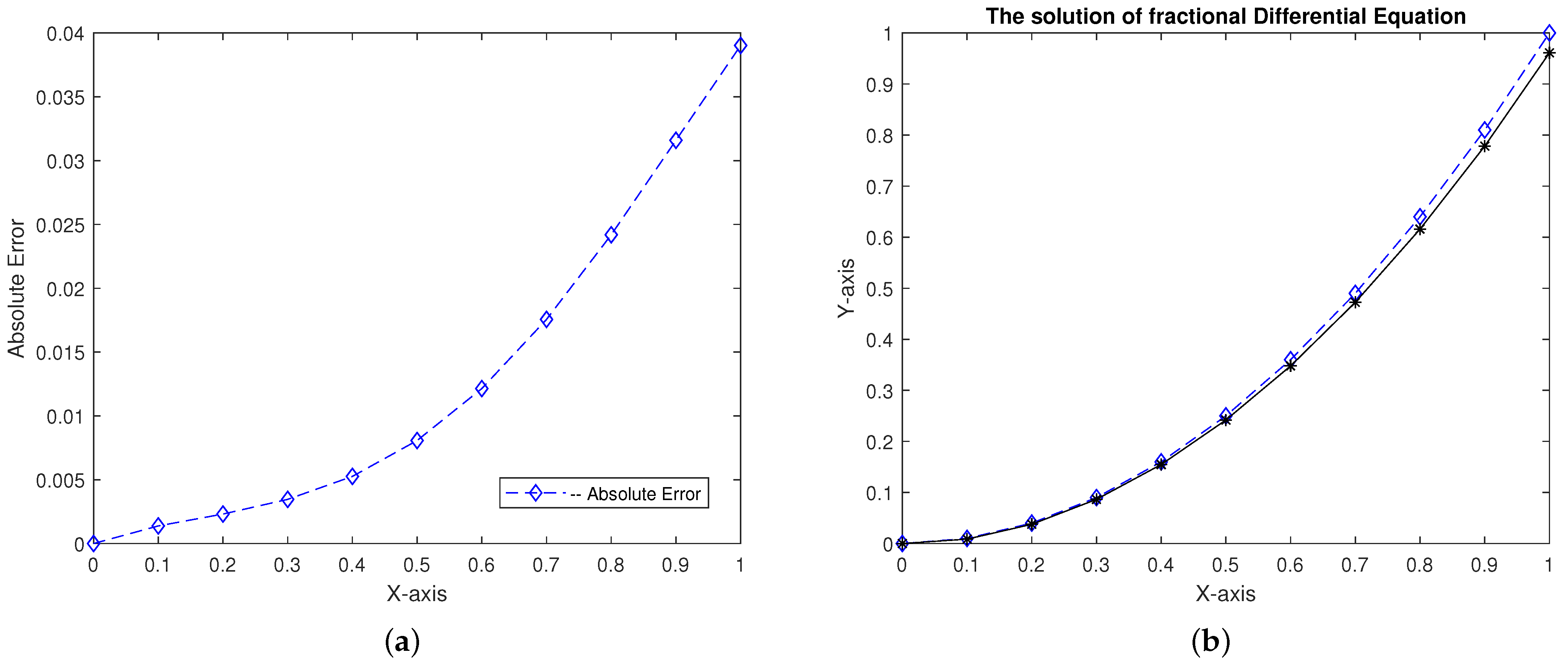
5. Application I

In this section, we study the existence and unique solution of integral equations as an application of Theorem 1.

Theorem 5.

Let us consider the integral equations

$$\begin{array}{c}\hfill 𝚤\left(\varpi \right)=\mathfrak{n}\left(\varpi \right)+{\int }_{{\mathcal{E}}_1\cup {\mathcal{E}}_2}{\mathcal{G}}_1(\varpi ,\varrho ,𝚤\left(\varrho \right))d\varrho ,\varpi \in {\mathcal{E}}_1\cup {\mathcal{E}}_2,\end{array}$$

$$\begin{array}{c}\hfill 𝚤\left(\varpi \right)=\mathfrak{n}\left(\varpi \right)+{\int }_{{\mathcal{E}}_1\cup {\mathcal{E}}_2}{\mathcal{G}}_2(\varpi ,\varrho ,𝚤\left(\varrho \right))d\varrho ,\varpi \in {\mathcal{E}}_1\cup {\mathcal{E}}_2,\end{array}$$

where ${\mathcal{E}}_1\cup {\mathcal{E}}_2$ is a Lebesgue measurable set. Suppose

• ${\mathcal{G}}_1,{\mathcal{G}}_2:({\mathcal{E}}_1^2\cup {\mathcal{E}}_2^2)\times [0,\infty )\to [0,\infty )$ and $b\in {\pounds }^{\infty }\left({\mathcal{E}}_1\right)\cup {\pounds }^{\infty }\left({\mathcal{E}}_2\right)$,
• $\rho \in (0,1)$ exists, such that

  $$\begin{array}{c}\hfill |{\mathcal{G}}_1(\varpi ,\varrho ,𝚤\left(\varrho \right))-{\mathcal{G}}_1(\varpi ,\varrho ,𝚥\left(\varrho \right)|\le \rho |{\mathcal{G}}_2(\varpi ,\varrho ,𝚤\left(\varrho \right))-{\mathcal{G}}_2(\varpi ,\varrho ,𝚥\left(\varrho \right)|,\end{array}$$

  for $\varpi ,\varrho \in {\mathcal{E}}_1^2\cup {\mathcal{E}}_2^2$.

Then, the integral equations have a unique common solution in ${\pounds }^{\infty }\left({\mathcal{E}}_1\right)\cup {\pounds }^{\infty }\left({\mathcal{E}}_2\right)$.

Proof. 

Let $\xi ={\pounds }^{\infty }\left({\mathcal{E}}_1\right)$ and ${\rm Y}={\pounds }^{\infty }\left({\mathcal{E}}_2\right)$ be two normed linear spaces, where ${\mathcal{E}}_1,{\mathcal{E}}_2$ are Lebesgue measurable sets and $m({\mathcal{E}}_1\cup {\mathcal{E}}_2)<\infty$. Let $\mathcal{H}={\pounds }^2\left({\mathcal{E}}_1\right)\cup {\pounds }^2\left({\mathcal{E}}_2\right)$. Consider $\partial :\xi \times {\rm Y}\to \pounds \left(\mathcal{H}\right)$ defined by $\partial (𝚤,𝚥)={\pi }_{|𝚤-𝚥|}$, where ${\pi }_{\mathfrak{h}}:\mathcal{H}\to \mathcal{H}$ is the multiplication operator defined by ${\pi }_{\mathfrak{h}}\left(\mathfrak{z}\right)=\mathfrak{h}.\mathfrak{z}$ for $\mathfrak{z}\in \mathcal{H}$. Then, $(\xi ,{\rm Y},\Lambda ,\partial )$ is a complete $C^{★}$-AVBMS.

Define the covariant mappings $\mathcal{W},\mathcal{V}:{\pounds }^{\infty }\left({\mathcal{E}}_1\right)\cup {\pounds }^{\infty }\left({\mathcal{E}}_2\right)\to {\pounds }^{\infty }\left({\mathcal{E}}_1\right)\cup {\pounds }^{\infty }\left({\mathcal{E}}_2\right)$ by

$$\begin{array}{c}\hfill \mathcal{W}\left(𝚤\left(\varpi \right)\right)=\mathfrak{n}\left(\varpi \right)+{\int }_{{\mathcal{E}}_1\cup {\mathcal{E}}_2}{\mathcal{G}}_1(\varpi ,\varrho ,𝚤\left(\varrho \right))d\varrho ,\varpi \in {\mathcal{E}}_1\cup {\mathcal{E}}_2.\end{array}$$

$$\begin{array}{c}\hfill \mathcal{V}\left(𝚤\left(\varpi \right)\right)=\mathfrak{n}\left(\varpi \right)+{\int }_{{\mathcal{E}}_1\cup {\mathcal{E}}_2}{\mathcal{G}}_2(\varpi ,\varrho ,𝚤\left(\varrho \right))d\varrho ,\varpi \in {\mathcal{E}}_1\cup {\mathcal{E}}_2.\end{array}$$

Setting $\mathcal{B}=\rho \mathfrak{T}$, then $\mathcal{B}\in \pounds {\left(\mathcal{H}\right)}_{+}$ and $\left|\right|\mathcal{B}\left|\right|=\rho <1$. For any $\mathfrak{h}\in \mathcal{H}$,

$$\begin{array}{cc}\hfill \left|\right|\partial (\mathcal{W}𝚤,\mathcal{W}𝚥)\left|\right|& =\underset{\parallel \mathfrak{h}\parallel =1}{sup}({\pi }_{|\mathcal{W}𝚤-\mathcal{W}𝚥|}\mathfrak{h},\mathfrak{h})\hfill \\ \hfill & =\underset{\parallel \mathfrak{h}\parallel =1}{sup}{\int }_{{\mathcal{E}}_1\cup {\mathcal{E}}_2}\left[{\int }_{{\mathcal{E}}_1\cup {\mathcal{E}}_2}|{\mathcal{G}}_1(\varpi ,\varrho ,𝚤\left(\varrho \right))-{\mathcal{G}}_1(\varpi ,\varrho ,𝚥\left(\varrho \right))|d\varrho \right]\mathfrak{h}\left(\varpi \right)\overline{\mathfrak{h}\left(\varpi \right)}d\varpi \hfill \\ \hfill & \le \underset{\parallel \mathfrak{h}\parallel =1}{sup}{\int }_{{\mathcal{E}}_1\cup {\mathcal{E}}_2}\left[{\int }_{{\mathcal{E}}_1\cup {\mathcal{E}}_2}\rho |{\mathcal{G}}_2(\varpi ,\varrho ,𝚤\left(\varrho \right))-{\mathcal{G}}_2(\varpi ,\varrho ,𝚥\left(\varrho \right))|d\varrho \right]|\mathfrak{h}\left(\varpi \right)\overline{\mathfrak{h}\left(\varpi \right)}d\varpi \hfill \\ \hfill & =\rho \underset{\parallel \mathfrak{h}\parallel =1}{sup}{\int }_{{\mathcal{E}}_1\cup {\mathcal{E}}_2}\left[{\int }_{{\mathcal{E}}_1\cup {\mathcal{E}}_2}|{\mathcal{G}}_2(\varpi ,\varrho ,𝚤\left(\varrho \right))-{\mathcal{G}}_2(\varpi ,\varrho ,𝚥\left(\varrho \right))|d\varrho \right]|\mathfrak{h}\left(\varpi \right)\overline{\mathfrak{h}\left(\varpi \right)}d\varpi \hfill \\ \hfill & \le \rho \left|\right|\partial (\mathcal{V}𝚤,\mathcal{V}𝚥)\left|\right|\hfill \\ \hfill & =\left|\right|\mathcal{B}\left|\right|\left|\right|\partial (\mathcal{V}𝚤,\mathcal{V}𝚥)\left|\right|.\hfill \end{array}$$

Since $\left|\right|\mathcal{B}\left|\right|<1$, all the hypotheses of Theorem 1 are verified. Hence, the integral equations have a unique common solution. □

6. Application II

Let $\overline{\varsigma }:[0,+\infty )\to \mathbb{R}$ be a continuous function. Next, we recall the definition of the Caputo derivative of the function $\overline{\varsigma }$ of the order $\overline{\beta }>0$ (see [19,20]):

$$\begin{array}{c}\hfill {}^{\mathbb{C}}\mathcal{D}\overline{\beta }\left(\overline{\varsigma }\left(\varpi \right)\right):=\frac{1}{\Gamma (\delta -\overline{\beta })}{\int }_0^{\varpi }{(\varpi -\varrho )}^{\delta -\overline{\beta }-1}{\overline{\varsigma }}^{\left(\delta \right)}\left(\varrho \right)d\varrho ,(\delta -1<\overline{\beta }<\delta ,\delta =\left[\overline{\beta }\right]+1),\end{array}$$

where $\left[\overline{\beta }\right]$ denotes the integer part of the positive real number $\overline{\beta }$, and $\Gamma$ is a gamma function. Consider the following nonlinear fractional differential equations

$$\begin{array}{c}\hfill {}^{\mathbb{C}}{\mathcal{D}}^{\overline{\beta }}\left(𝚤\left(\varpi \right)\right)+{\mathcal{W}}_1(\varpi ,𝚤\left(\varpi \right))=0,(0\le \varpi \le 1,\overline{\beta }<1)\end{array}$$

(7)

and

$$\begin{array}{c}\hfill {}^{\mathbb{C}}{\mathcal{D}}^{\overline{\beta }}\left(𝚤\left(\varpi \right)\right)+{\mathcal{W}}_2(\varpi ,𝚤\left(\varpi \right))=0,(0\le \varpi \le 1,\overline{\beta }<1)\end{array}$$

(8)

with the boundary conditions $𝚤\left(0\right)=0=𝚤\left(1\right)$. Let $\xi =\overline{\mathbb{C}}([0,1],[0,+\infty ))$ be the space of all continuous functions defined on the interval $[0,1]$ with values in the interval $[0,+\infty )$ and ${\rm Y}=\overline{\mathbb{C}}([0,1],(-\infty ,0])$ be the space of all continuous functions defined on the interval $[0,1]$ with values in the interval $(-\infty ,0]$. Let $\Lambda ={\mathcal{M}}_2\left(\mathbb{C}\right)$ and $\partial :\xi \times {\rm Y}\to {\Lambda }_{+}$ be defined by

$$\partial (𝚤,𝚥)=\left[\begin{array}{c}\begin{array}{cc}\underset{\varpi \in [0,1]}{sup}|𝚤\left(\varpi \right)-𝚥\left(\varpi \right)|& 0\\ 0& \mathbb{k}\underset{\varpi \in [0,1]}{sup}|𝚤\left(\varpi \right)-𝚥\left(\varpi \right)|\end{array}\end{array}\right]$$

for all $𝚤\in \xi$ and $𝚥\in {\rm Y}$, where $\mathbb{k}\ge 0$ is a constant. Then, $(\xi ,{\rm Y},\Lambda ,\partial )$ is a complete $C^{★}$-AVBMS. The nonlinear fractional differential Equations (7) and (8) can be written in integral form as

$$\begin{array}{c}\hfill 𝚤\left(\varpi \right)={\int }_0^1\theta (\varpi ,\varrho ){\mathcal{W}}_1(\varrho ,𝚤\left(\varrho \right))d\varrho \mathrm{for}\mathrm{all}\varpi \in [0,1]\end{array}$$

and

$$\begin{array}{c}\hfill 𝚤\left(\varpi \right)={\int }_0^1\theta (\varpi ,\varrho ){\mathcal{W}}_2(\varrho ,𝚤\left(\varrho \right))d\varrho \mathrm{for}\mathrm{all}\varpi \in [0,1],\end{array}$$

where $\theta (\varpi ,\varrho ):{[0,1]}^2\to \mathbb{R}$ is a Green’s function associated with (7) and (8), we obtain

$$\begin{array}{c}\hfill \theta (\varpi ,\varrho )=\left\{\begin{array}{c}{\left(\varpi (1-\varrho )\right)}^{\alpha -1}-{(\varpi -\varrho )}^{\alpha -1},\mathrm{if}0\le \varrho \le \varpi \le 1\hfill \\ \frac{{\left(\varpi (1-\varrho )\right)}^{\alpha -1}}{\Gamma \left(\alpha \right)},\mathrm{if}0\le \varpi \le \varrho \le 1.\hfill \end{array}\right.\end{array}$$

Theorem 6.

Let $\mathcal{V},\mathcal{W}$ be a self-mapping on $(\Phi ,\Psi ,\mathcal{H},\phi )$, such that

(i) 

θ is the Green’s function;

(ii) 

${\mathcal{W}}_1,{\mathcal{W}}_2:[0,1]\times \mathbb{R}\to \mathbb{R}$ are continuous functions such that $\forall (𝚤,𝚥)\in (\xi ,{\rm Y})$, we have the inequality

$$\begin{array}{c}\hfill |{\mathcal{W}}_1(\varrho ,𝚤\left(\varrho \right))-{\mathcal{W}}_1(\varrho ,𝚥\left(\varrho \right))|\le \frac{1}{3}|{\mathcal{W}}_2(\varrho ,𝚤\left(\varrho \right))-{\mathcal{W}}_2(\varrho ,𝚥\left(\varrho \right))|.\end{array}$$

Then, the nonlinear fractional differential Equations (7) and (8) have a unique common solution.

Proof. 

Define $\mathcal{V},\mathcal{W}:\xi \cup {\rm Y}\to \xi \cup {\rm Y}$ by

$$\begin{array}{c}\hfill \mathcal{W}𝚤\left(\varpi \right)={\int }_0^1\theta (\varpi ,\varrho ){\mathcal{W}}_1(\varrho ,𝚤\left(\varrho \right))d\varrho \end{array}$$

and

$$\begin{array}{c}\hfill \mathcal{V}𝚤\left(\varpi \right)={\int }_0^1\theta (\varpi ,\varrho ){\mathcal{W}}_2(\varrho ,𝚤\left(\varrho \right))d\varrho .\end{array}$$

Let $𝚤\in \xi$. Then,

$$\begin{array}{cc}\hfill \mathcal{V}𝚤\left(\varpi \right)& ={\int }_0^1\theta (\varpi ,\varrho ){\mathcal{W}}_1(\varrho ,𝚤\left(\varrho \right))d\varrho \hfill \\ \hfill & \in \xi .\hfill \end{array}$$

Let $𝚥\in {\rm Y}$. Then,

$$\begin{array}{cc}\hfill \mathcal{V}𝚥\left(\varpi \right)& ={\int }_0^1\theta (\varpi ,\varrho ){\mathcal{W}}_2(\varrho ,𝚤\left(\varrho \right))d\varrho \hfill \\ \hfill & \in {\rm Y}.\hfill \end{array}$$

Therefore, $\mathcal{V}$ is a covariant mapping. Similarly, we can prove that $\mathcal{W}$ is a covariant mapping. Now,

$$\begin{array}{cc}\hfill & \partial (\mathcal{W}𝚤,\mathcal{W}𝚥)=\left[\begin{array}{c}\begin{array}{cc}\underset{\varpi \in [0,1]}{sup}|\mathcal{W}𝚤\left(\varpi \right)-\mathcal{W}𝚥\left(\varpi \right)|& 0\\ 0& \mathbb{k}\underset{\varpi \in [0,1]}{sup}|\mathcal{W}𝚤\left(\varpi \right)-\mathcal{W}𝚥\left(\varpi \right)|\end{array}\end{array}\right]\hfill \\ \hfill & \le \left[\begin{array}{cc}& \begin{array}{cc}\underset{\varpi \in [0,1]}{sup}{\int }_0^1\theta (\varpi ,\varrho )|{\mathcal{W}}_1(\varrho ,𝚤\left(\varrho \right))-{\mathcal{W}}_1(\varrho ,𝚥\left(\varrho \right))|d\varrho & 0\\ 0& \mathbb{k}\underset{\varpi \in [0,1]}{sup}{\int }_0^1\theta (\varpi ,\varrho )|{\mathcal{W}}_1(\varrho ,𝚤\left(\varrho \right))-{\mathcal{W}}_1(\varrho ,𝚥\left(\varrho \right))|d\varrho \end{array}\end{array}\right]\hfill \\ \hfill & \le \left[\begin{array}{cc}& \begin{array}{cc}\underset{\varpi \in [0,1]}{sup}{\int }_0^1\theta (\varpi ,\varrho )\frac{1}{3}|{\mathcal{W}}_2(\varrho ,𝚤\left(\varrho \right))-{\mathcal{W}}_2(\varrho ,𝚥\left(\varrho \right))|d\varrho & 0\\ 0& \mathbb{k}\underset{\varpi \in [0,1]}{sup}{\int }_0^1\theta (\varpi ,\varrho )\frac{1}{3}|{\mathcal{W}}_2(\varrho ,𝚤\left(\varrho \right))-{\mathcal{W}}_2(\varrho ,𝚥\left(\varrho \right))|d\varrho \end{array}\end{array}\right]\hfill \\ \hfill & ={\rho }^{★}\partial (\mathcal{V}𝚤,\mathcal{V}𝚥)\rho ,\hfill \end{array}$$

where

$$\rho =\left[\begin{array}{c}\begin{array}{cc}\frac{1}{\sqrt{3}}& 0\\ 0& \frac{1}{\sqrt{3}}\end{array}\end{array}\right]$$

and $\left|\right|\rho \left|\right|=\frac{1}{\sqrt{3}}<1$. Therefore,

$$\begin{array}{c}\hfill \partial (\mathcal{W}𝚤,\mathcal{W}𝚥)\le {\rho }^{★}\partial (\mathcal{V}𝚤,\mathcal{V}𝚥)\rho .\end{array}$$

Hence, all the hypotheses of Theorem 1 are fulfilled. Hence, the nonlinear fractional differential Equations (7) and (8) have a unique common solution. □

7. Application III

We recall some elementary definitions from the theory of fractional calculus. For a function $\mathfrak{z}\in \mathcal{C}[0,1]$, the Reiman–Liouville fractional derivative of order $\overline{\beta }>0$ is given by

$$\begin{array}{c}\hfill \frac{1}{\Gamma (\delta -\overline{\beta })}\frac{d^{\delta }}{d{\varpi }^{\delta }}{\int }_0^{\varpi }\frac{𝚤\left(\mathfrak{c}\right)d\mathfrak{c}}{{(\varpi -\mathfrak{c})}^{\overline{\beta }-\delta +1}}={\mathcal{D}}^{\overline{\beta }𝚤\left(\varpi \right)},\end{array}$$

provided that the right hand side is pointwise defined on $[0,1]$, where $\left[\overline{\beta }\right]$ is the integer part of the number $\overline{\beta },and \Gamma$ is the Euler gamma function.

Consider the following fractional differential equation

$$\begin{array}{cc}\hfill & {}^{\mathfrak{c}}{\mathcal{D}}^{\xi }𝚤\left(\varpi \right)+\mathfrak{f}(\varpi ,𝚤\left(\varpi \right))=0,1\le \varpi \le 0,2\le \xi >1;\hfill \\ \hfill & 𝚤\left(0\right)=𝚤\left(1\right)=0,\hfill \end{array}$$

(9)

where $\mathfrak{f}$ is a continuous function from $[0,1]\times \mathbb{R}$ to $\mathbb{R}$ and ${}^{\mathfrak{c}}{\mathcal{D}}^{\xi }$ represents the Caputo fractional derivative of order $\xi$, and it is defined by

$$\begin{array}{c}\hfill {}^{\mathfrak{c}}{\mathcal{D}}^{\xi }=\frac{1}{\Gamma (\delta -\xi )}{\int }_0^{\varpi }\frac{{𝚤}^{\delta }\left(\mathfrak{c}\right)d\mathfrak{c}}{{(\varpi -\mathfrak{c})}^{\xi -\delta +1}}\end{array}$$

Let $\xi =\left(\mathcal{C}\right[0,1],[0,\infty \left)\right)$ be the set of all continuous functions defined on $[0,1]$ with values in the interval $[0,\infty )$ and ${\rm Y}=\left(\mathcal{C}\right[0,1],(-\infty ,0\left]\right)$ be the set of all continuous functions defined on $[0,1]$ with values in the interval $(-\infty ,0]$. Let $\Lambda ={\mathcal{M}}_2\left(\mathbb{C}\right)$ and $\partial :\xi \times {\rm Y}\to {\Lambda }_{+}$ be defined by

$$\partial (𝚤,𝚥)=\left[\begin{array}{c}\begin{array}{cc}\underset{\varpi \in [0,1]}{sup}|𝚤\left(\varpi \right)-𝚥\left(\varpi \right)|& 0\\ 0& \mathbb{k}\underset{\varpi \in [0,1]}{sup}|𝚤\left(\varpi \right)-𝚥\left(\varpi \right)|\end{array}\end{array}\right]$$

for all $𝚤\in \xi$ and $𝚥\in {\rm Y}$, where $\mathbb{k}\ge 0$ is a constant. Then, $(\xi ,{\rm Y},\Lambda ,\partial )$ is a complete $C^{★}$-AVBMS.

Theorem 7.

Consider the nonlinear fractional differential Equation (9). Suppose that the following assertions are satisfied:

(i) 

$\varpi \in [0,1]$, $\rho \in [0,1]$ and $(𝚤,{𝚤}^{{}^{\prime }})\in \xi \times {\rm Y}$ exist, such that

$$\begin{array}{c}\hfill |\mathfrak{f}(\varpi ,𝚤)-\mathfrak{f}(\varpi ,{𝚤}^{{}^{\prime }})|\le \rho (|{𝚤}^{{}^{\prime }}\left(\varpi \right)-\mathcal{W}{𝚤}^{{}^{\prime }}\left(\varpi \right)|+|\mathcal{W}𝚤\left(\varpi \right)-𝚤\left(\varpi \right)\left|\right);\end{array}$$

(ii) 

$$\begin{array}{c}\hfill \underset{\varpi \in [0,1]}{sup}{\int }_0^1\left|\mathcal{G}(\varpi ,\mathfrak{c})\right|d\mathfrak{c}\le 1.\end{array}$$

Then, the fractional differential Equation (9) has a unique solution in $\xi \cup {\rm Y}$.

Proof. 

The given fractional differential Equation (9) is equivalent to the succeeding integral equation

$$\begin{array}{c}\hfill 𝚤\left(\varpi \right)={\int }_0^1\mathcal{G}(\varpi ,\mathfrak{c})\mathfrak{f}(\mathfrak{s},𝚤\left(\mathfrak{c}\right))d\mathfrak{c},\end{array}$$

where

$$\begin{array}{c}\hfill \mathcal{G}(\varpi ,\mathfrak{c})=\left\{\begin{array}{cc}\frac{{\left[\varpi (1-\mathfrak{c})\right]}^{\xi -1}-{(\varpi -\mathfrak{c})}^{\xi -1}}{\Gamma \left(\xi \right)},\hfill & 0\le \mathfrak{c}\le \varpi \le 1,\hfill \\ \frac{{\left[\varpi (1-\mathfrak{c})\right]}^{\xi -1}}{\Gamma \left(\xi \right)},\hfill & 0\le \varpi \le \mathfrak{c}\le 1.\hfill \end{array}\right.\end{array}$$

Define the contravariant mapping $\mathcal{W}:\xi \cup {\rm Y}\to \xi \cup {\rm Y}$ defined by

$$\begin{array}{c}\hfill \mathcal{W}𝚤\left(\varpi \right)={\int }_0^1\mathcal{G}(\varpi ,\mathfrak{c})\mathfrak{f}(\mathfrak{s},𝚤\left(\mathfrak{c}\right))d\mathfrak{c}.\end{array}$$

Now,

$$\begin{array}{cc}\hfill & \partial (\mathcal{W}𝚥,\mathcal{W}𝚤)=\left[\begin{array}{c}\begin{array}{cc}\underset{\varpi \in [0,1]}{sup}|\mathcal{W}𝚥\left(\varpi \right)-\mathcal{W}𝚤\left(\varpi \right)|& 0\\ 0& \mathbb{k}\underset{\varpi \in [0,1]}{sup}|\mathcal{W}𝚥\left(\varpi \right)-\mathcal{W}𝚤\left(\varpi \right)|\end{array}\end{array}\right]\hfill \\ \hfill & \le \left[\begin{array}{cc}& \begin{array}{cc}\underset{\varpi \in [0,1]}{sup}{\int }_0^1\mathcal{G}(\varpi ,\mathfrak{c})|\mathfrak{f}(\mathfrak{s},𝚥\left(\mathfrak{c}\right))-\mathfrak{f}(\mathfrak{s},𝚤\left(\mathfrak{c}\right))|d\mathfrak{c}& 0\\ 0& \mathbb{k}\underset{\varpi \in [0,1]}{sup}{\int }_0^1\mathcal{G}(\varpi ,\mathfrak{c})|\mathfrak{f}(\mathfrak{s},𝚥\left(\mathfrak{c}\right))-\mathfrak{f}(\mathfrak{s},𝚤\left(\mathfrak{c}\right))|d\mathfrak{c}\end{array}\end{array}\right]\hfill \\ \hfill & \le \left[\begin{array}{cc}& \begin{array}{cc}\underset{\varpi \in [0,1]}{sup}{\int }_0^1\mathcal{G}(\varpi ,\mathfrak{c})\rho \left(\right|𝚤\left(\varpi \right)-\mathcal{W}𝚤\left(\varpi \right)|+|\mathcal{W}𝚥\left(\varpi \right)-𝚥\left(\varpi \right)\left|\right)d\mathfrak{c}& 0\\ 0& \mathbb{k}\underset{\varpi \in [0,1]}{sup}{\int }_0^1\mathcal{G}(\varpi ,\mathfrak{c})\rho \left(\right|𝚤\left(\varpi \right)-\mathcal{W}𝚤\left(\varpi \right)|\\ & +\left|\mathcal{W}𝚥\right(\varpi )-𝚥(\varpi \left)\right|)d\mathfrak{c}\end{array}\end{array}\right]\hfill \\ \hfill & =\rho (\partial (𝚤,\mathcal{W}𝚤)+\partial (\mathcal{W}𝚥,𝚥\left)\right).\hfill \end{array}$$

Therefore,

$$\begin{array}{c}\hfill \partial (\mathcal{W}𝚥,\mathcal{W}𝚤)⪯\rho (\partial (𝚤,\mathcal{W}𝚤)+\partial (\mathcal{W}𝚥,𝚥\left)\right)\mathrm{for}\mathrm{all}𝚤\in \xi ,𝚥\in {\rm Y},\end{array}$$

Hence, all the hypotheses of Corollary 1 are verified, and consequently, the fractional differential Equation (9) has a unique solution. □

Example 3.

The linear fractional differential equation is as follows:

$$\begin{array}{c}\hfill {\mathcal{D}}^{\overline{\beta }}𝚤\left(\varpi \right)+𝚤\left(\varpi \right)={\displaystyle \frac{2}{\Gamma (3-\overline{\beta })}}{\varpi }^{2-\overline{\beta }}+{\varpi }^3,\end{array}$$

(10)

with the initial condition $𝚤\left(0\right)=0,{𝚤}^{\prime }\left(0\right)=0$.

Equation (10) has an exact solution with $\overline{\beta }=1.9$:

$$\begin{array}{c}\hfill 𝚤\left(\varpi \right)={\varpi }^2\end{array}$$

By Equation (9), we can express Equation (10) in the homotopy form:

$$\begin{array}{c}\hfill {\mathcal{D}}^{\overline{\beta }}𝚤\left(\varpi \right)+\mathfrak{u}𝚤\left(\varpi \right)-{\displaystyle \frac{2}{\Gamma (3-\overline{\beta })}}{\varpi }^{2-\overline{\beta }}-{\varpi }^3=0,\end{array}$$

(11)

The solution to Equation (10) is:

$$\begin{array}{c}\hfill 𝚤\left(\varpi \right)={𝚤}_0\left(\varpi \right)+\mathfrak{u}{𝚤}_1\left(\varpi \right)+{\mathfrak{u}}^2{𝚤}_2\left(\varpi \right)+\cdots .\end{array}$$

(12)

By substituting Equation (12) into (11) and collecting terms with the power of $\mathfrak{u}$, we obtain

$$\begin{array}{c}\hfill \left\{\begin{array}{cc}{\mathfrak{u}}^0:\hfill & {\mathcal{D}}^{\overline{\beta }}{𝚤}_0\left(\varpi \right)=0\hfill \\ {\mathfrak{u}}^1:\hfill & {\mathcal{D}}^{\overline{\beta }}{𝚤}_1\left(\varpi \right)=-{𝚤}_0\left(\varpi \right)+\mathfrak{f}\left(\varpi \right)\hfill \\ {\mathfrak{u}}^2:\hfill & {\mathcal{D}}^{\overline{\beta }}{𝚤}_2\left(\varpi \right)=-{𝚤}_1\left(\varpi \right)\hfill \\ {\mathfrak{u}}^3:\hfill & {\mathcal{D}}^{\overline{\beta }}{𝚤}_3\left(\varpi \right)=-{𝚤}_2\left(\varpi \right)\hfill \end{array}\begin{array}{c}\hfill ⋮.\end{array}\right.\end{array}$$

(13)

By applying ${{\rm Y}}^{\overline{\beta }}$ and the inverse operation of ${\mathcal{D}}^{\overline{\beta }}$ to both sides of Equation (13) and the fractional integral operation $\left({{\rm Y}}^{\overline{\beta }}\right)$ of order $\overline{\beta }>0$, we have

$$\begin{array}{cc}\hfill {𝚤}_0\left(\varpi \right)& =\sum _{\mathfrak{i}=0}^1{𝚤}^{\mathfrak{i}}\left(0\right){\displaystyle \frac{{\varpi }^{\mathfrak{i}}}{\mathfrak{i}!}}\hfill \\ & =𝚤\left(0\right){\displaystyle \frac{{\varpi }^0}{0!}}+{𝚤}^{\prime }\left(0\right){\displaystyle \frac{{\varpi }^1}{1!}}\hfill \\ \hfill {𝚤}_1\left(\varpi \right)& =-{{\rm Y}}^{\overline{\beta }}\left[{𝚤}_0\left(\varpi \right)+{{\rm Y}}^{\overline{\beta }}\left[\mathfrak{f}\left(\varpi \right)\right]\right]\hfill \\ & ={\varpi }^2+{\displaystyle \frac{\Gamma \left(4\right)}{\Gamma (4+\overline{\beta })}}{\varpi }^{3+\overline{\beta }},\hfill \\ \hfill {𝚤}_2\left(\varpi \right)& =-{{\rm Y}}^{\overline{\beta }}\left[{𝚤}_1\left(\varpi \right)\right]\hfill \\ & ={\displaystyle \frac{2}{\Gamma (3+\overline{\beta })}}{\varpi }^{2+\overline{\beta }}-{\displaystyle \frac{6}{\Gamma (3+2\overline{\beta })}}{\varpi }^{3+2\overline{\beta }},\hfill \\ \hfill {𝚤}_3\left(\varpi \right)& =-{{\rm Y}}^{\overline{\beta }}\left[{𝚤}_2\left(\varpi \right)\right]\hfill \\ & ={\displaystyle \frac{2}{\Gamma (3+2\overline{\beta })}}{\varpi }^{2+2\overline{\beta }}-{\displaystyle \frac{6}{\Gamma (3+3\overline{\beta })}}{\varpi }^{3+3\overline{\beta }}.\hfill \end{array}$$

Hence, the solution to Equation (10) is

$$\begin{array}{cc}\hfill 𝚤\left(\varpi \right)& ={𝚤}_0\left(\varpi \right)+{𝚤}_1\left(\varpi \right)+{𝚤}_2\left(\varpi \right)+\cdots \hfill \end{array}$$

(14)

$$\begin{array}{cc}\hfill 𝚤\left(\varpi \right)& ={\varpi }^2+{\displaystyle \frac{\Gamma \left(4\right)}{\Gamma (4+\overline{\beta })}}{\varpi }^{(3+\overline{\beta })}-{\displaystyle \frac{2}{\Gamma (3+\overline{\beta })}}{\varpi }^{(2+\overline{\beta })}-{\displaystyle \frac{6}{\Gamma (4+2\overline{\beta })}}{\varpi }^{(3+2\overline{\beta })}+\cdots ,\hfill \end{array}$$

(15)

when $\overline{\beta }=1.9$

$$\begin{array}{cc}\hfill 𝚤\left(\varpi \right)& ={\varpi }^2+{\displaystyle \frac{6}{\Gamma \left(5.9\right)}}{\varpi }^{\left(4.9\right)}-{\displaystyle \frac{2}{\Gamma \left(4.9\right)}}{\varpi }^{\left(3.9\right)}-{\displaystyle \frac{6}{\Gamma \left(7.8\right)}}{\varpi }^{\left(6.8\right)}+\cdots \hfill \\ & ={\varpi }^2-\mathrm{small}\mathrm{terms}\hfill \\ & \approx {\varpi }^2.\hfill \end{array}$$

Table 1. The numerical and exact solutions obtained using the matrix approach method where $\xi$ = 51.

$\mathit{\varpi }$	$𝚤\left(\mathit{\varpi }\right)$	${𝚤}_{\mathit{\xi }}\left(\mathit{\varpi }\right)$	Error
0.05	0.0025	0.738759	0.736259
0.15	0.0225	0.808072	0.785572
0.25	0.0625	0.823676	0.761176
0.35	0.1225	0.820716	0.698216
0.45	0.2025	0.811879	0.609379
0.55	0.3025	0.805843	0.503343
0.65	0.4225	0.809961	0.387461
0.75	0.5625	0.831017	0.268517
0.85	0.7225	0.875504	0.153004
0.95	0.9025	0.949759	0.047259

: displays the numerical and exact results using the matrix approach method with $\overline{\beta }=1.9$ and ξ = 51. The maximum error with $\xi =51$ is $0.039016195358901$.

Figure 1a compares both the numerical and exact solutions for the fractional differential Equation (10). Moreover, Figure 1b shows the absolute error between the numerical and exact solutions.

8. Conclusions

We proved common fixed point theorems under different contractive mappings on ${\mathbb{C}}^{★}$-algebra-valued bipolar metric spaces. An illustrative example was provided to demonstrate the validity of the hypothesis and the degree of utility of our findings. Additionally, as an application of our results, we showed that some classes of nonlinear fractional differential equations with the boundary conditions have a unique common solution. This concept can be applied for further investigations of ${\mathbb{C}}^{★}$-algebra-valued bipolar metric spaces for other structures in metric spaces.

References

- Mutlu, A.; Gürdal, U. Bipolar metric spaces and some fixed point theorems. J. Nonlinear Sci. Appl. 2016, 9, 5362–5373. [Google Scholar] [CrossRef] [Green Version]
- Gürdal, U.; Mutlu, A.; Özkan, K. Fixed point results for ψ-ϕ ontractive mappings in bipolar metric spaces. J. Inequalities Spec. Funct. 2020, 11, 64–75. [Google Scholar]
- Kishore, G.N.V.; Agarwal, R.P.; Rao, B.S.; Rao, R.V.N.S. Caristi type cyclic contraction and common fixed point theorems in bipolar metric spaces with applications. Fixed Point Theory Appl. 2018, 2018, 21. [Google Scholar] [CrossRef] [Green Version]
- Kishore, G.N.V.; Prasad, D.R.; Rao, B.S.; Baghavan, V.S. Some applications via common coupled fixed point theorems in bipolar metric spaces. J. Crit. Rev. 2019, 7, 601–607. [Google Scholar]
- Kishore, G.N.V.; Rao, K.P.R.; Sombabu, A.; Rao, R.V.N.S. Related results to hybrid pair of mappings and applications in bipolar metric spaces. J. Math. 2019, 2019, 8485412. [Google Scholar] [CrossRef]
- Rao, B.S.; Kishore, G.N.V.; Kumar, G.K. Geraghty type contraction and common coupled fixed point theorems in bipolar metric spaces with applications to homotopy. Int. Math. Trends Technol. 2018, 63, 25–34. [Google Scholar] [CrossRef] [Green Version]
- Kishore, G.N.V.; Rao, K.P.R.; Işik, H.; Rao, B.S.; Sombabu, A. Covarian mappings and coupled fixed point results in bipolar metric spaces. Int. J. Nonlinear Anal. Appl. 2021, 12, 1–15. [Google Scholar]
- Mutlu, A.; Özkan, K.; Gürdal, U. Locally and weakly contractive principle in bipolar metric spaces. TWMS J. Appl. Eng. Math. 2020, 10, 379–388. [Google Scholar]
- Gaba, Y.U.; Aphane, M.; Aydi, H. Contractions in Bipolar Metric Spaces. J. Math. 2021, 2021, 5562651. [Google Scholar] [CrossRef]
- Ma, Z.H.; Jiang, L.N.; Sun, H.K. C*-algebras-valued metric spaces and related fixed point theorems. Fixed Point Theory Appl. 2014, 206, 222. [Google Scholar] [CrossRef] [Green Version]
- Batul, S.; Kamran, T. C★-valued contractive type mappings. Fixed Point Theory Appl. 2015, 2015, 142. [Google Scholar] [CrossRef] [Green Version]
- Gunaseelan, M.; Arul Joseph, G.; Ul Haq, A.; Baloch, I.A.; Jarad, F. Coupled fixed point theorems on C★-algebra-valued bipolar metric spaces. AIMS Math. 2022, 7, 7552–7568. [Google Scholar]
- Gunaseelan, M.; Arul Joseph, G.; Işik, H.; Jarad, F. Fixed point results in C★-algebra-valued bipolar metric spaces with an application. AIMS Math. 2023, 8, 7695–7713. [Google Scholar]
- Ramaswamy, R.; Mani, G.; Gnanaprakasam, A.J.; Abdelnaby, O.A.A.; Stojiljković, V.; Radojevic, S.; Radenović, S. Fixed points on covariant and contravariant maps with an application. Mathematics 2022, 10, 4385. [Google Scholar] [CrossRef]
- Davidson, K.R. C★-Algebras by Example. In Fields Institute Monographs; Springer: Berlin/Heidelberg, Germany, 1996; Volume 6. [Google Scholar]
- Murphy, G.J. C*-Algebra and Operator Theory; Academic Press: London, UK, 1990. [Google Scholar]
- Xu, Q.H.; Bieke, T.E.D.; Chen, Z.Q. Introduction to Operator Algebras and Non Commutative Lp Spaces; Science Press: Beijing, China, 2010. (In Chinese) [Google Scholar]
- Douglas, R.G. Banach Algebra Techniques in Operator Theory; Springer: Berlin/Heidelberg, Germany, 1998. [Google Scholar]
- Kilbas, A.A.; Srivastava, H.M.; Trujillo, J.J. Theory and Applications of Fractional Differential Equations. In North-Holland Mathematics Studies; Elsevier: Amsterdam, The Netherlands, 2006; Volume 204. [Google Scholar]
- Samko, S.G.; Kilbas, A.A.; Marichev, O.I. Fractional Integral and Derivative; Gordon and Breach: London, UK, 1993. [Google Scholar]