Fractal Dimension of Fractal Functions on the Real Projective Plane

Abstract

In this article, we consider an iterated functions system on the non-Euclidean real projective plane which has a linear structure. Then, we study the fractal dimension of the associated curve as a subset of the projective space and like a set of the Euclidean space. At the end, we initiate a dual real projective iterated function system and pose an open problem.

1. Introduction

Fractals are those geometric objects on abstract spaces that own some kind of self-similarity. The best-known example of the fractal set is called the Mandelbrot set, named after the mathematician Benoit Mandelbrot who coined the term fractal [1]. In geometry, one of the most important methods to construct fractals is based on iterated function systems (IFSs). Based on some historical precedents, Hutchinson [2] introduced IFSs to generate self-similar sets. Barnsley [3] used another tool to construct fractals as the graphs of self-referential functions, known as fractal interpolation functions (FIFs). Most of the authors studied fractal interpolation on the Euclidean spaces [4,5,6,7,8]. Recently, Barnsley et al. [9], studied IFSs on the real projective plane. Hossain et al. [10] introduced the real projective fractal interpolation function ( RPFIF) by considering a real projective iterated function system (RPIFS) on the projective plane.

In mathematics, given a Euclidean space ${\mathbb{R}}^{n+1}$, the real projective space associated with ${\mathbb{R}}^{n+1}$ is the collection of all one-dimensional subspaces or (vector) lines in ${\mathbb{R}}^{n+1}$, and is denoted by ${\mathbb{RP}}^n$. One can identify ${\mathbb{RP}}^n$ as the quotient of the set ${\mathbb{R}}^{n+1}\setminus \left\{0\right\}$ of non-zero vectors by the equivalence relation $x\sim y$ if and only if $x=\lambda y$ for some $\lambda \in {\mathbb{R}}^{*}$ (non-zero reals). Now, for $x=(x_1,x_2,\dots ,x_{n+1})\in {\mathbb{R}}^{n+1}\setminus \left\{0\right\}$, we denote $(x_1:x_2:\dots :x_{n+1})$ as the equivalence class containing x. Thus, there exists a canonical map $\nu :{\mathbb{R}}^{n+1}\setminus \left\{0\right\}\to {\mathbb{RP}}^n$ that associates each non-zero vector $x=(x_1,x_2,\dots ,x_{n+1})\in {\mathbb{R}}^{n+1}\setminus \left\{0\right\}$ with the element $(x_1:x_2:\dots :x_{n+1})\in {\mathbb{RP}}^n$. The points $(x_1,x_2,\dots ,x_{n+1})\in {\mathbb{R}}^{n+1}\setminus \left\{0\right\}$ such that $\nu (x_1,x_2,\dots ,x_{n+1})=p$ is referred to as homogeneous coordinates of an element $p\in {\mathbb{RP}}^n$. If $p,q\in {\mathbb{RP}}^n$ have the homogeneous coordinates $(p_1,p_2,\dots ,p_{n+1})$ and $(q_1,q_2,\dots ,q_{n+1})$, respectively, and ${\sum }_{k=1}^{n+1}{p}_k{q}_k=0$, then we say that p is orthogonal to q, and write $p\perp q$. A hyperplane in ${\mathbb{RP}}^n$ is a set of the form

$${\mathbb{H}}_p=\left\{q\in {\mathbb{RP}}^n:p\perp q\right\}\subseteq {\mathbb{RP}}^n$$

for some $p\in {\mathbb{RP}}^n$. A set $\mathbb{K}\subseteq {\mathbb{RP}}^n$ is said to avoid a hyperplane if there exists a hyperplane ${\mathbb{H}}_p\subseteq {\mathbb{RP}}^n$ such that ${\mathbb{H}}_p\cap \mathbb{K}=\varnothing$. A line in the real projective space is the set of equivalence classes of points in a two-dimensional subspace of ${\mathbb{R}}^{n+1}$. Here, we recall a few notations and results from one of our earlier works [10]. Consider the hyperplane ${\mathbb{H}}_{e_3}$ where $e_3=(0:0:1)$ and the space ${\mathbb{RP}}^2\setminus {\mathbb{H}}_{e_3}$ in particular, defining two operations ⊕ and ⊙ as follows. For all $(x:y:z),(x^{\prime }:y^{\prime }:z^{\prime })\in {\mathbb{RP}}^2\setminus {\mathbb{H}}_{e_3}$ and for all $a\in \mathbb{R}$,

$$(x:y:z)\oplus (x^{\prime }:y^{\prime }:z^{\prime }):=(x{z}^{\prime }+x^{\prime }z:y{z}^{\prime }+y^{\prime }z:z{z}^{\prime })$$

(1)

and

$$a\odot (x:y:z):=(ax:ay:z).$$

(2)

${\mathbb{RP}}^2\setminus {\mathbb{H}}_{e_3}$ forms a vector space over $\mathbb{R}$ with respect to the operations ⊕ and ⊙. Use the notation ⊖ to indicate the difference between two elements in ${\mathbb{RP}}^2\setminus {\mathbb{H}}_{e_3}$. That is, if $(x_1:y_1:z_1),(x_2:y_2:z_2)\in {\mathbb{RP}}^2\setminus {\mathbb{H}}_{e_3}$, then $(x_1:y_1:z_1)\ominus (x_2:y_2:z_2)=(x_1{z}_2-x_2{z}_1:y_1{z}_2-y_2{z}_1:z_1{z}_2)$. So, each element $(x:y:z)$ in ${\mathbb{RP}}^2\setminus {\mathbb{H}}_{e_3}$ can be expressed as a sum of two of its elements, namely $(x:0:z)$ and $(0:y:z)$. That is, $(x:y:z)=(x:0:z)\oplus (0:y:z)$. Let ${\mathbb{H}}_{10}:=\left\{(x:0:z)\in {\mathbb{RP}}^2\setminus {\mathbb{H}}_{e_3}\right\}$ and ${\mathbb{H}}_{01}:=\left\{(0:y:z)\in {\mathbb{RP}}^2\setminus {\mathbb{H}}_{e_3}\right\}$. Then, ${\mathbb{RP}}^2\setminus {\mathbb{H}}_{e_3}$ can be expressed as

$${\mathbb{RP}}^2\setminus {\mathbb{H}}_{e_3}={\mathbb{H}}_{10}\oplus {\mathbb{H}}_{01}.$$

(3)

Define a norm on ${\mathbb{RP}}^2\setminus {\mathbb{H}}_{e_3}$, called a projective norm, as follows:

$${\parallel (x:y:z)\parallel }_{\mathbb{P}}:=\frac{\sqrt{x^2+y^2}}{\left|z\right|}$$

(4)

for all $(x:y:z)\in {\mathbb{RP}}^2\setminus {\mathbb{H}}_{e_3}$. The projective norm induces a metric which is denoted by $d_{\mathbb{P}}$. The space ${\mathbb{RP}}^2\setminus {\mathbb{H}}_{e_3}$ is complete with respect to this norm. For $(x_1:0:z_1),(x_2:0:z_2)\in {\mathbb{H}}_{10}$, denote that $(x_1:0:z_1)⪯(x_2:0:z_2)$, if and only if $x_1{z}_2\le x_2{z}_1$, and $(x_1:0:z_1)\prec (x_2:0:z_2)$, if and only if $x_1{z}_2<x_2{z}_1$. Similarly for $(0:y_1:z_1),(0:y_2:z_2)\in {\mathbb{H}}_{01}$, define $(0:y_1:z_1)⪯(0:y_2:z_2)$, if and only if $y_1{z}_2\le y_2{z}_1$, and $(0:y_1:z_1)\prec (0:y_2:z_2)$, if and only if $y_1{z}_2<y_2{z}_1$.

Definition 1 

(Projective intervals on ${\mathbb{H}}_{10}$ and ${\mathbb{H}}_{01}$ [10]). Let $(a_1:0:c_1),(a_2:0:c_2)\in {\mathbb{H}}_{10}$ be such that $(a_1:0:c_1)\prec (a_2:0:c_2)$. Then, the projective interval on ${\mathbb{H}}_{10}$ is denoted by ${\mathbb{P}}_{I\times \left\{0\right\}}$ and defined by

$$\begin{array}{c}\hfill {\mathbb{P}}_{I\times \left\{0\right\}}:={\displaystyle \{}(x:0:z)\in {\mathbb{H}}_{10}:(a_1:0:c_1)⪯(x:0:z)⪯(a_2:0:c_2){\displaystyle \}}.\end{array}$$

Similarly, the projective interval on ${\mathbb{H}}_{01}$, is denoted by ${\mathbb{P}}_{\left\{0\right\}\times J}$ and defined by

$$\begin{array}{c}\hfill {\mathbb{P}}_{\left\{0\right\}\times J}:={\displaystyle \{}(0:y:z)\in {\mathbb{H}}_{01}:(0:b_1:d_1)⪯(0:y:z)⪯(0:b_2:d_2){\displaystyle \}}.\end{array}$$

Definition 2 

(Projective rectangle [10]). Let $(a_1:0:c_1),(a_2:0:c_2)\in {\mathbb{H}}_{10}$ and $(0:b_1:d_1),(0:b_2:d_2)\in {\mathbb{H}}_{01}$ be such that $(a_1:0:c_1)\prec (a_2:0:c_2)$ and $(0:b_1:d_1)\prec (0:b_2:d_2)$. Then, the projective rectangle on ${\mathbb{RP}}^2\setminus {\mathbb{H}}_{e_3}$ is defined by

$$\begin{array}{cc}\hfill {\mathbb{P}}_{I\times J}:={\displaystyle \{}(x:y:z)\in {\mathbb{RP}}^2\setminus {\mathbb{H}}_{e_3}& :(a_1:0:c_1)⪯(x:0:z)⪯(a_2:0:c_2)\hfill \\ \hfill & and(0:b_1:d_1)⪯(0:y:z)⪯(0:b_2:d_2){\displaystyle \}}.\hfill \end{array}$$

Let $\mathcal{C}\left[{\mathbb{P}}_{I\times \left\{0\right\}}\right]=\left\{f:{\mathbb{P}}_{I\times \left\{0\right\}}\to {\mathbb{H}}_{01}\mathrm{continuous}\right\}.$ If $f\in \mathcal{C}\left[{\mathbb{P}}_{I\times \left\{0\right\}}\right]$, define ${\parallel f\parallel }_{\mathbb{P}\infty }:={sup\{\parallel f(x:0:z)\parallel }_{\mathbb{P}}:(x:0:z)\in {\mathbb{P}}_{I\times \left\{0\right\}}\}$. Since ${\mathbb{P}}_{I\times \left\{0\right\}}$ is compact, ${\parallel f\parallel }_{\mathbb{P}\infty }$ is well defined. For more details, interested readers may consult [10].

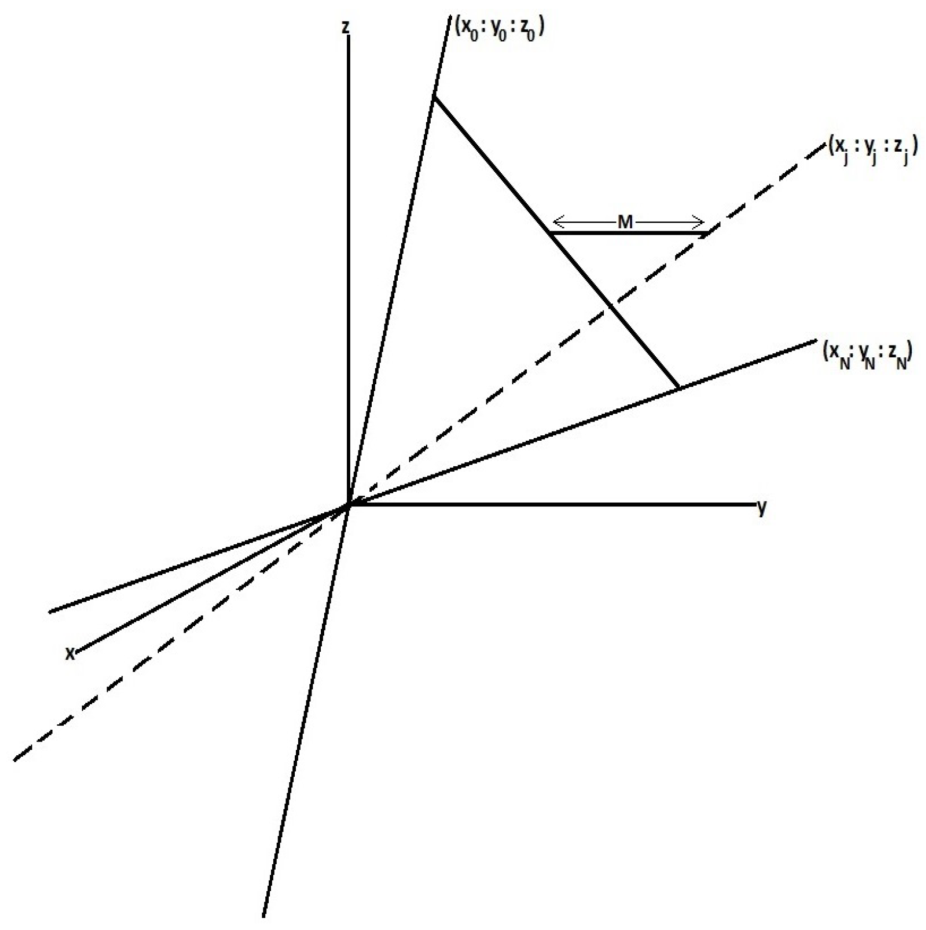
Let $N\ge 2$ and $\left\{(x_n:y_n:z_n)\in {\mathbb{RP}}^2\setminus {\mathbb{H}}_{e_3}:n=0,1,\dots ,N\right\}$ be a dataset in ${\mathbb{RP}}^2\setminus {\mathbb{H}}_{e_3}$ such that $x_n{z}_{n+1}<x_{n+1}{z}_n$ for $n=0,1,\dots ,N-1$. Let ${\mathbb{P}}_{I\times \left\{0\right\}}:=\left\{(x:0:z)\in {\mathbb{H}}_{10}:(x_0:0:z_0)⪯(x:0:z)⪯(x_N:0:z_N)\right\}$ and ${\mathbb{P}}_{I_n\times \left\{0\right\}}:=\left\{(x:0:z)\in {\mathbb{H}}_{10}:(x_{n-1}:0:z_{n-1})⪯(x:0:z)⪯(x_n:0:z_n)\right\}$ for $n=1,2,\dots ,N$. For $n=1,2,\dots ,N$, consider the transformations $L_n:{\mathbb{P}}_{I\times \left\{0\right\}}\to {\mathbb{P}}_{I_n\times \left\{0\right\}}$ given by $L_n(x:0:z)=(a_{n}x+b_{n}z:0:z)$ such that

$$L_n(x_0:0:z_0)=(x_{n-1}:0:z_{n-1})and{L}_n(x_N:0:z_N)=(x_n:0:z_n),$$

(5)

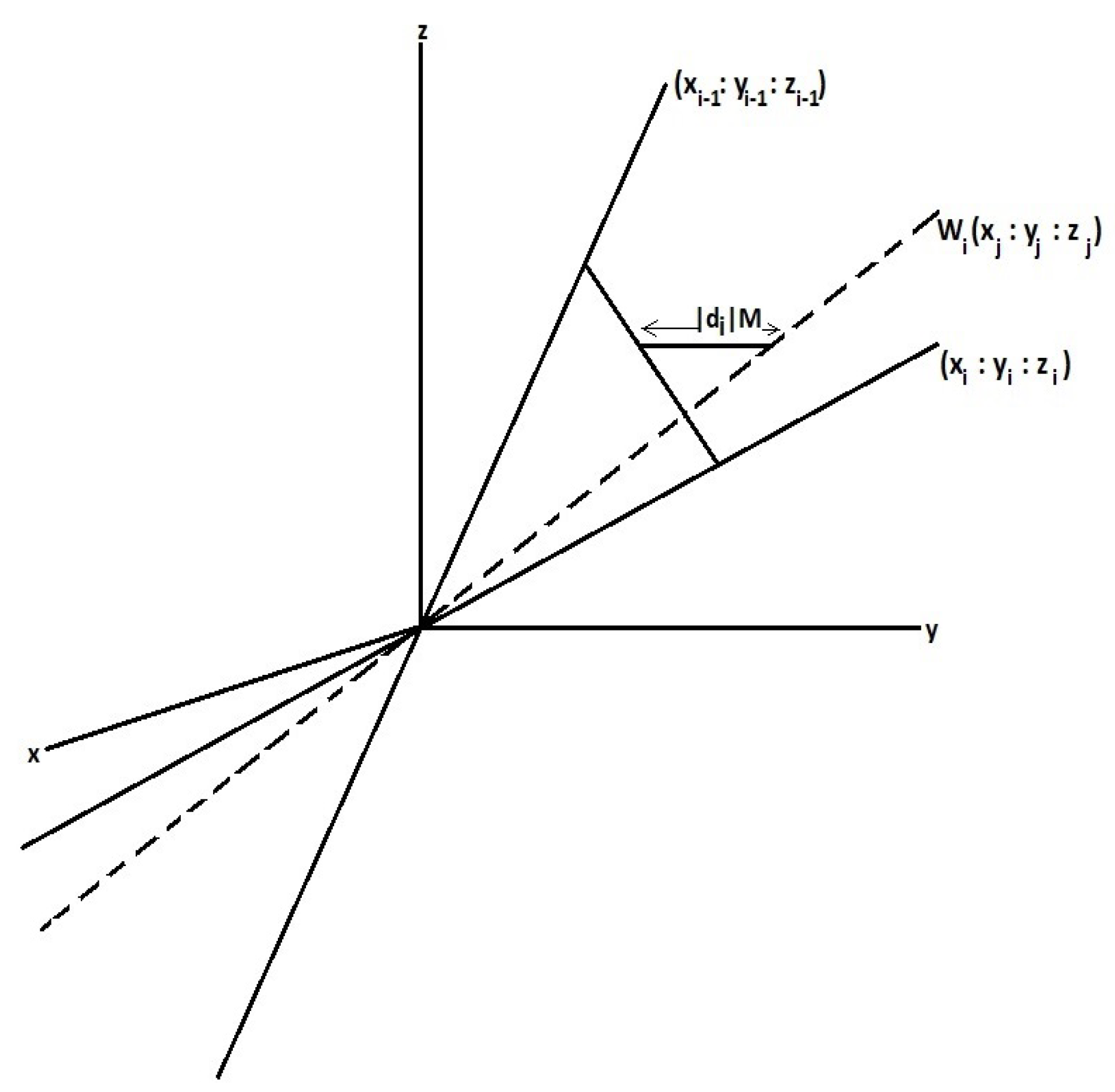
where $a_n,b_n\in \mathbb{R}$. Then $L_n$’s are contraction maps with respect to the metric $d_{\mathbb{P}}$. For $n=1,2,\dots ,N$, consider the continuous maps $F_n:{\mathbb{RP}}^2\setminus {\mathbb{H}}_{e_3}\to {\mathbb{H}}_{01}$ given by

$$F_n(x:y:z)=\left(0:c_{n}x+d_{n}y+f_{n}z:z\right)$$

(6)

such that

$$F_n(x_0:y_0:z_0)=(0:y_{n-1}:z_{n-1})and{F}_n(x_N:y_N:z_N)=(0:y_n:z_n),$$

(7)

where $c_n,d_n,f_n\in \mathbb{R}$. If $d_n<1$, then $F_n$’s are contractive with respect to the second variable. Now, for $n=1,2,\dots ,N$, define the functions $W_n:{\mathbb{RP}}^2\setminus {\mathbb{H}}_{e_3}\to {\mathbb{RP}}^2\setminus {\mathbb{H}}_{e_3}$ by

$$W_n(x:y:z)=L_n(x:0:z)\oplus F_n(x:y:z).$$

(8)

The transformation $W_n$s are known as projective transformations, (as can be seen in [9,10]).

Theorem 1 

([10]). The RPIFS $\left\{{\mathbb{RP}}^2\setminus {\mathbb{H}}_{e_3};W_n:n=1,2,\dots ,N\right\}$ has a unique attractor, which is the graph of a continuous function from ${\mathbb{P}}_{I\times \left\{0\right\}}$ to ${\mathbb{H}}_{01}$.

This function is known as RPFIF on a real projective plane.

The fractal dimension, which is in the heart of the fractal geometry, is usually considered in connection with real world data. It measures the complexity of a geometric shape in the space and it also provides an objective procedure in order to numerically compare the fractal sets. It may also be seen as a measure of the space-filling capacity of a pattern. The fractal dimension may not be an integer. In the literature, the concept of several dimensions of the fractal sets with respect to the Euclidean distance on the plane was largely treated (as can be seen, for instance, in [5,6,11,12,13,14,15,16,17,18]).

In this article, on the basis of these concepts, we estimate the fractal dimension of the graph of an RPFIF. As the graph of an RPFIF can be viewed as a subset of the real projective plane ${\mathbb{RP}}^2$ as well as a subset of ${\mathbb{R}}^3$, the dimensions are estimated in both cases. The topological dimension of the projective plane ${\mathbb{RP}}^2$ is two and the dimension of ${\mathbb{R}}^3$ is three. In this article, we prove that, if D is the dimension of the graph of RPFIF in ${\mathbb{RP}}^2$, then $D+1$ is the dimension of it in ${\mathbb{R}}^3$.

One of the interesting features of the projective geometry is that of duality. In projective geometry, the dual of a point is a line and the dual of a line is a point. Dual space is the collection of all the hyperplanes of a projective space. It is used in many branches of mathematics, such as tensor analysis with the finite dimensional spaces, measure distribution, and Hilbert spaces [19]. At the end of this article, an open problem concerning the dual RPFIF is posed.

2. Fractal Dimension of the Graph of a RPFIF

In this section, we estimate the fractal dimension of the graph G of an RPFIF when the interpolation points are equispaced. The following definition is used for the estimation of the dimensions.

Definition 3 

(see [6,11]). Let $r>0$ and $\mathcal{N}\left(r\right)$ denote the minimum number of balls of radius r needed to cover a set F. Then, the fractal dimension of the set F, is denoted by ${dim}_{B}F$, and defined by

$$\underset{r\to 0}{lim}\frac{log\mathcal{N}\left(r\right)}{logr},ifitexists.$$

2.1. Fractal Dimension of the Graph of an RPFIF as a Subset of ${\mathbb{RP}}^2\setminus {\mathbb{H}}_{e_3}$

Let ${\mathbb{P}}_{I\times \left\{0\right\}}=\left\{(x:0:z)\in {\mathbb{H}}_{10}:(0:0:1)⪯(x:0:z)⪯(1:0:1)\right\}$ and $X={\mathbb{P}}_{I\times \left\{0\right\}}\oplus {\mathbb{H}}_{01}$ and let $N\ge 2$, and $\{(x_i:y_i:z_i):i=0,1,2,\dots ,N\}$ be the $N+1$ interpolation points in X such that $(x_i:0:z_i)\ominus (x_{i-1}:0:z_{i-1})=(1:0:N)$. That is, the points $(x_i:0:z_i)$ are equally spaced. Define a hyperbolic RPIFS $\{(X;W_i):i=1,2,\dots ,N\}$ such that

$$\begin{array}{c}\hfill W_i\left(\begin{array}{c}x\\ y\\ z\end{array}\right)=\left(\begin{array}{ccc}1& 0& i-1\\ N{c}_i& N{d}_i& N{k}_i\\ 0& 0& N\end{array}\right)\left(\begin{array}{c}x\\ y\\ z\end{array}\right),\end{array}$$

(9)

where $\left(\begin{array}{c}x\\ y\\ z\end{array}\right)$ represents the element $(x:y:z)$ in ${\mathbb{RP}}^2\setminus {\mathbb{H}}_{e_3}$. Now, each $W_i$ can be written as

$$\begin{array}{cc}\hfill W_i(x:y:z)& =(x+(i-1)z:N(c_{i}x+d_{i}y+k_{i}z):Nz)\hfill \\ \hfill & =(x+(i-1)z:0:Nz)\oplus \left(0:N(c_{i}x+d_{i}y+k_{i}z):Nz\right)\hfill \\ \hfill & =(x+(i-1)z:0:Nz)\oplus \left(0:c_{i}x+d_{i}y+k_{i}z:z\right)\hfill \\ \hfill & =L_i(x:0:z)\oplus F_i(x:y:z),\hfill \end{array}$$

where $L_i(x:0:z)=(x+(i-1)z:0:Nz)$, $F_i(x:y:z)=\left(0:c_{i}x+d_{i}y+k_{i}z:z\right),$ the values of $c_i$, $k_i$ are given by (5), and (7) and $d_i$ are the free parameters for $i=1,2,\dots ,N$. If the free parameters $d_i$ are such that $\left|d_i\right|<1$, then the maps $W_i$, $i\in \{1,2,\dots ,N\}$ are contractive. Hence, the above RPIFS possesses a unique attractor which is the graph of a continuous function $\mathbf{f}:{\mathbb{P}}_{I\times \left\{0\right\}}\to {\mathbb{H}}_{01}$ passing through the data points $(x_i:0:z_i)$, $i\in \{0,1,2,\dots ,N\}$. Let G be the graph of $\mathbf{f}$. That is

$$G={\displaystyle \{}(x:0:z)\oplus \mathbf{f}(x:0:z):(x:0:z)\in {\mathbb{P}}_{I\times \left\{0\right\}}{\displaystyle \}}.$$

For $k,r\in \mathbb{N}$ and $\alpha =(0:{\alpha }_1:{\alpha }_2)\in {\mathbb{RP}}^2\setminus {\mathbb{H}}_{e_3}$, consider the projective intervals

$$\begin{array}{cc}\hfill & {\mathbb{P}}_{I_k\times \left\{0\right\}}={\displaystyle \{}(x:0:z)\in {\mathbb{P}}_{I\times \left\{0\right\}}:(k-1:0:N^r)⪯(x:0:z)⪯(k:0:N^r){\displaystyle \}}\hfill \\ \hfill & \mathrm{and}\hfill \\ \hfill & {\mathbb{P}}_{\left\{0\right\}\times J_{\alpha }}={\displaystyle \{}(0:y:z)\in {\mathbb{RP}}^2\setminus {\mathbb{H}}_{e_3}:(0:{\alpha }_1:{\alpha }_2)⪯(0:y:z)⪯(0:N^r{\alpha }_1+{\alpha }_2:N^r{\alpha }_2){\displaystyle \}}\hfill \end{array}$$

on ${\mathbb{H}}_{10}$ and ${\mathbb{H}}_{01}$, respectively. Let

$$\begin{array}{c}\hfill {\mathcal{C}}_{\mathbb{P}}=\left\{{\mathbb{P}}_{I_k\times \left\{0\right\}}\oplus {\mathbb{P}}_{\left\{0\right\}\times J_{\alpha }}:k,r\in \mathbb{N}and\alpha =(0:{\alpha }_1:{\alpha }_2)\in {\mathbb{RP}}^2\setminus {\mathbb{H}}_{e_3}\right\}.\end{array}$$

Now, it can be seen that ${\mathbb{P}}_{I_k\times \left\{0\right\}}\oplus {\mathbb{P}}_{\left\{0\right\}\times J_{\alpha }}={\mathbb{P}}_{I_k\times J_{\alpha }}$, and ${\parallel (k:0:N^r)\ominus (k-1:0:N^r)\parallel }_{\mathbb{P}}={\parallel (1:0:N^r)\parallel }_{\mathbb{P}}=\frac{1}{N^r}$ and ${\parallel (0:N^r{\alpha }_1+{\alpha }_2:N^r{\alpha }_2)\ominus (0:{\alpha }_1:{\alpha }_2)\parallel }_{\mathbb{P}}={\parallel (0:1:N^r)\parallel }_{\mathbb{P}}=\frac{1}{N^r}$. Thus, the length of the projective intervals are $|{\mathbb{P}}_{I_k\times \left\{0\right\}}|=|{\mathbb{P}}_{\left\{0\right\}\times J_{\alpha }}|=\frac{1}{N^r}$. Therefore, ${\mathcal{C}}_{\mathbb{P}}$ is the collection of projective squares of side length $\frac{1}{N^r}$ on ${\mathbb{RP}}^2\setminus {\mathbb{H}}_{e_3}$.

Let ${\mathcal{N}}_{\mathbb{P}}^{*}\left(r\right)$ be the minimum number of $\frac{1}{N^r}\times \frac{1}{N^r}$ projective squares in ${\mathcal{C}}_{\mathbb{P}}$ entailed to cover G and let ${\mathcal{N}}_{\mathbb{P}}\left(r\right)$ be the smallest number of $\frac{1}{N^r}\times \frac{1}{N^r}$ projective squares in X which covers G. Then, it is clear that ${\mathcal{N}}_{\mathbb{P}}\left(r\right)\le {\mathcal{N}}_{\mathbb{P}}^{*}\left(r\right)$. Now, any $\frac{1}{N^r}\times \frac{1}{N^r}$ projective squares in X can be covered by two $\frac{1}{N^r}\times \frac{1}{N^r}$ projective squares in ${\mathcal{C}}_{\mathbb{P}}$. Therefore, $2{\mathcal{N}}_{\mathbb{P}}\left(r\right)\ge {\mathcal{N}}_{\mathbb{P}}^{*}\left(r\right)$. Thus, for dimension calculation, it is sufficient to focus on

$$\begin{array}{c}\hfill \underset{r\to \infty }{lim}\frac{log{\mathcal{N}}_{\mathbb{P}}^{*}\left(r\right)}{log{N}^r}.\end{array}$$

Before proving the main result in this section, we prove the following lemma.

Lemma 1. 

If all the interpolation points are not collinear in ${\mathbb{RP}}^2\setminus {\mathbb{H}}_{e_3}$ and $\mu ={\sum }_{i=1}^N\left|d_i\right|>1$, then

$$\underset{r\to \infty }{lim}\frac{{\mathcal{N}}_{\mathbb{P}}^{*}\left(r\right)}{N^r}=\infty .$$

Proof. 

For any $(x:y:z)\in {\mathbb{RP}}^2\setminus {\mathbb{H}}_{e_3}$, we can write $(x:y:z)=(\frac{x}{z}:\frac{y}{z}:1)$. Then, the line equation joining the points $(x_0:y_0:z_0)=(\frac{x_0}{z_0}:\frac{y_0}{z_0}:1)$ and $(x_N:y_N:z_N)=(\frac{x_N}{z_N}:\frac{y_N}{z_N}:1)$ on the plane $z=1$ is given by

$$\begin{array}{cc}\hfill & \frac{\frac{y}{z}-\frac{y_0}{z_0}}{\frac{x}{z}-\frac{x_0}{z_0}}=\frac{\frac{y_N}{z_N}-\frac{y_0}{z_0}}{\frac{x_N}{z_N}-\frac{x_0}{z_0}}\hfill \\ \hfill & \frac{y}{z}=\frac{y_0}{z_0}+\left(\frac{x}{z}-\frac{x_0}{z_0}\right)\left(\frac{\frac{y_N}{z_N}-\frac{y_0}{z_0}}{\frac{x_N}{z_N}-\frac{x_0}{z_0}}\right).\hfill \end{array}$$

Now, $(x_0:0:z_0)=(0:0:1)$ and $(x_N:0:z_N)=(1:0:1)$, so, $\frac{x_0}{z_0}=0$, $\frac{x_N}{z_N}=1$. Therefore,

$$\begin{array}{c}\hfill \frac{y}{z}=\frac{y_0}{z_0}+\frac{x}{z}\left(\frac{y_N}{z_N}-\frac{y_0}{z_0}\right).\end{array}$$

(10)

Hence, from (10), the line equation on ${\mathbb{RP}}^2\setminus {\mathbb{H}}_{e_3}$ can be written as

$$\begin{array}{cc}\hfill p(x:0:z)& =(0:\frac{y_0}{z_0}:1)\oplus \left(0:\frac{x}{z}\left(\frac{y_N}{z_N}-\frac{y_0}{z_0}\right):1\right)\hfill \\ \hfill & =(0:y_0:z_0)\oplus \frac{x}{z}\odot \left((0:y_N:z_N)\ominus (0:y_0:z_0)\right).\hfill \end{array}$$

As the interpolation points are not collinear in ${\mathbb{RP}}^2\setminus {\mathbb{H}}_{e_3}$, there exists a $j\in \{1,2,\dots ,N\}$ such that

$$\begin{array}{c}\hfill M={\parallel \mathbf{f}(x_j:0:z_j)\ominus p(x_j:0:z_j)\parallel }_{\mathbb{P}}>0.\end{array}$$

This gives

$$\begin{array}{c}\hfill M={{\displaystyle \parallel }\left((0:y_j:z_j)\ominus (0:y_0:z_0)\right)\ominus \left(\frac{x_j}{z_j}\odot \left((0:y_N:z_N)\ominus (0:y_0:z_0)\right)\right){\displaystyle \parallel }}_{\mathbb{P}}>0.\end{array}$$

(see Figure 1). Clearly,

$$M\le max\left\{{\parallel (0:y_j:z_j)\ominus (0:y_0:z_0)\parallel }_{\mathbb{P}},{\parallel (0:y_j:z_j)\ominus (0:y_N:z_N)\parallel }_{\mathbb{P}}\right\}.$$

Since G is the graph of a continuous function, therefore,

$$\frac{{\mathcal{N}}_{\mathbb{P}}^{*}\left(r\right)}{N^r}\ge \left[M\right],$$

where $\left[M\right]$ denotes the greatest integer not greater than M. If we apply $W_i$ on G, then the length M switches to the length $\left|d_i\right|M$, $i\in \{1,2,\dots ,N\}$ (see Figure 2). Thus, we obtain

Figure 1. Non-collinear interpolation points in ${\mathbb{RP}}^2\setminus {\mathbb{H}}_{e_3}$.

Figure 1. Non-collinear interpolation points in ${\mathbb{RP}}^2\setminus {\mathbb{H}}_{e_3}$.

Figure 2. Effect of $W_i$ on the data points.

Figure 2. Effect of $W_i$ on the data points.

$$\frac{{\mathcal{N}}_{\mathbb{P}}^{*}\left(r\right)}{N^r}\ge \sum _{i=1}^N\left[\left|d_i\right|M\right]forr\ge 1.$$

By induction

$$\frac{{\mathcal{N}}_{\mathbb{P}}^{*}\left(r\right)}{N^r}\ge \sum _{i_1=1}^N\sum _{i_2=1}^N\cdots \sum _{i_k=1}^N\left[|d_{i_1}{d}_{i_2}\cdots d_{i_k}|M\right]forr\ge k.$$

Hence

$$\frac{{\mathcal{N}}_{\mathbb{P}}^{*}\left(r\right)}{N^r}\ge M{\left(\sum _{i=1}^N\left|d_i\right|\right)}^r-1=M{\mu }^r-1.$$

(11)

As $\mu >1$, taking the limit as $r\to \infty$, we obtain

$$\begin{array}{c}\hfill \underset{r\to \infty }{lim}\frac{{\mathcal{N}}_{\mathbb{P}}^{*}\left(r\right)}{N^r}=\infty .\end{array}$$

□

Theorem 2. 

If $G=graph\left(\mathbf{f}\right)$, $\mu ={\sum }_{i=1}^N\left|d_i\right|>1$ and the interpolation points are not collinear, then ${dim}_B\left(G\right)=1+{log}_N\mu$; otherwise, ${dim}_B\left(G\right)=1$.

Proof. 

Let ${\mathcal{C}}_{\mathbb{P}}\left(r\right)\in {\mathcal{C}}_{\mathbb{P}}$ be a “finest" cover of G consisting of ${\mathcal{N}}_{\mathbb{P}}^{*}\left(r\right)$$\frac{1}{N^r}\times \frac{1}{N^r}$ projective squares of ${\mathcal{C}}_{\mathbb{P}}$ and let ${\mathcal{C}}_{\mathbb{P}}(r,k)$ denote the collection of all projective squares in ${\mathcal{C}}_{\mathbb{P}}$ which lie between $(k-1:0:N^r)$ and $(k:0:N^r)$. Let ${\mathcal{N}}_{\mathbb{P}}(r,k)$ denote the number of projective squares in ${\mathcal{C}}_{\mathbb{P}}(r,k)$ and

$$\begin{array}{c}\hfill {\Lambda }_{\mathbb{P}}(r,k)=\bigcup _{{\mathcal{A}}_i\in {\mathcal{C}}_{\mathbb{P}}(r,k)}{\mathcal{A}}_i.\end{array}$$

As ${\mathcal{C}}_{\mathbb{P}}\left(r\right)$ is the finest cover of G, every projective square in ${\mathcal{C}}_{\mathbb{P}}\left(r\right)$ must intersect with G and since G is the graph of a continuous function, ${\Lambda }_{\mathbb{P}}(r,k)$ must be a projective rectangle of width $\frac{1}{N^r}$ and height $\frac{{\mathcal{N}}_{\mathbb{P}}(r,k)}{N^r}$. Furthermore, note that

$${\mathcal{N}}_{\mathbb{P}}^{*}\left(r\right)=\sum _{k=1}^{N^r}{\mathcal{N}}_{\mathbb{P}}(r,k).$$

(12)

Now, we estimate that ${\mathcal{N}}_{\mathbb{P}}^{*}(r+1)$ in terms of ${\mathcal{N}}_{\mathbb{P}}^{*}\left(r\right)$. Since

$$\begin{array}{c}\hfill L_i(k:0:N^r)=\left(k+(i-1)N^r:0:N^{r+1}\right)=\left(l(k,i):0:N^{r+1}\right),\end{array}$$

where $l(k,i)=k+(i-1)N^r$. It follows that

$$\begin{array}{cc}\hfill \parallel & L_i(k:0:N^r)\ominus L_i(k-1:0:N^r){\parallel }_{\mathbb{P}}\hfill \\ \hfill & ={\parallel (l(k,i):0:N^{r+1})\ominus (l(k,i)-1:0:N^{r+1})\parallel }_{\mathbb{P}}\hfill \\ \hfill & =\frac{1}{N^{r+1}}.\hfill \end{array}$$

(13)

Also, for $(x:y:z),(x^{\prime }:y^{\prime }:z^{\prime })\in {\Lambda }_{\mathbb{P}}(r,k)$,

$$\begin{array}{cc}\hfill \parallel & F_i(x:y:z)\ominus F_i(x^{\prime }:y^{\prime }:z^{\prime }){\parallel }_{\mathbb{P}}\hfill \\ \hfill & =(0:c_i(x{z}^{\prime }-x^{\prime }z)+d_i(y{z}^{\prime }-y^{\prime }z):z{z}^{\prime }){\parallel }_{\mathbb{P}}\hfill \\ \hfill & \le \left|c_i\right|\frac{|x{z}^{\prime }-x^{\prime }z|}{|z{z}^{\prime }|}+\left|d_i\right|\frac{|y{z}^{\prime }-y^{\prime }z|}{\left|z{z}^{\prime }\right|}\hfill \\ \hfill & =\left|c_i\right|{\parallel (x:0:z)\ominus (x^{\prime }:0:z^{\prime })\parallel }_{\mathbb{P}}+\left|d_i\right|{\parallel (0:y:z)\ominus (0:y^{\prime }:z^{\prime })\parallel }_{\mathbb{P}}\hfill \\ \hfill & \le \frac{\left|c_i\right|}{N^r}+\frac{\left|d_i\right|{\mathcal{N}}_{\mathbb{P}}(r,k)}{N^r}.\hfill \end{array}$$

This shows that $W_i\left({\Lambda }_{\mathbb{P}}(r,k)\right)$ is contained in a projective rectangle of width $\frac{1}{N^{r+1}}$ and height $\frac{\left|c_i\right|}{N^r}+\frac{\left|d_i\right|{\mathcal{N}}_{\mathbb{P}}(r,k)}{N^r}$. Therefore,

$$\begin{array}{cc}\hfill {\mathcal{N}}_{\mathbb{P}}(r+1,l(k,i))& \le \frac{\frac{\left|c_i\right|}{N^r}+\frac{\left|d_i\right|{\mathcal{N}}_{\mathbb{P}}(r,k)}{N^r}}{\frac{1}{N^{r+1}}}+1\hfill \\ \hfill & =N\left(\left|c_i\right|+\left|d_i\right|{\mathcal{N}}_{\mathbb{P}}(r,k)\right)+1.\hfill \end{array}$$

This yields,

$$\begin{array}{cc}\hfill {\mathcal{N}}_{\mathbb{P}}^{*}(r+1)& =\sum _{i=1}^N\sum _{k=1}^{N^r}{\mathcal{N}}_{\mathbb{P}}(r+1,l(k,i))\hfill \\ \hfill & \le N^{r+1}(1+\sum _{i=1}^N\left|c_i\right|)+N\sum _{i=1}^N\left|d_i\right|{\mathcal{N}}_{\mathbb{P}}^{*}\left(r\right)\hfill \\ \hfill & =N^{r+1}\delta +N\mu {\mathcal{N}}_{\mathbb{P}}^{*}\left(r\right),\hfill \end{array}$$

(14)

where $\delta =1+{\sum }_{i=1}^N\left|c_i\right|$. From (14), we obtain

$$\begin{array}{cc}\hfill {\mathcal{N}}_{\mathbb{P}}^{*}\left(r\right)\le N^r\delta +N\mu {\mathcal{N}}_{\mathbb{P}}^{*}(r-1)& \le N^r\delta +N\mu \left(N^{r-1}\delta +N\mu {\mathcal{N}}_{\mathbb{P}}^{*}(r-2)\right)\hfill \\ \hfill & =N^r{\delta (1+\mu )+\left(N\mu \right)}^2{\mathcal{N}}_{\mathbb{P}}^{*}(r-2)\hfill \end{array}$$

Therefore, the induction over r gives

$$\begin{array}{c}\hfill {\mathcal{N}}_{\mathbb{P}}^{*}\left(r\right)\le N^r\delta \left(1+\mu +{\mu }^2+\cdots +{\mu }^{r-1}\right)+{\left(N\mu \right)}^r{\mathcal{N}}_{\mathbb{P}}^{*}\left(1\right).\end{array}$$

(15)

Case 1. If $\mu \le 1$, then ${\mu }^r\le 1$ for all $r\in \mathbb{N}$. This implies that $1+\mu +{\mu }^2+\cdots +{\mu }^{r-1}\le r$. Furthermore, ${\mu }^r\le 1\le r$. Therefore, from (15), we obtain

$$\begin{array}{c}\hfill {\mathcal{N}}_{\mathbb{P}}^{*}\left(r\right)\le r{N}^r\delta +r{N}^r{\mathcal{N}}_{\mathbb{P}}^{*}\left(1\right)=r{N}^r{C}_2,\end{array}$$

where $C_2=\delta +{\mathcal{N}}_{\mathbb{P}}^{*}\left(1\right)$. Hence,

$$\begin{array}{c}\hfill {dim}_B\left(G\right)=\underset{r\to 0}{lim}\frac{log{\mathcal{N}}^{*}\left(r\right)}{logr}\le \underset{r\to \infty }{lim}\frac{log\left(r{N}^r{C}_2\right)}{log{N}^r}=1.\end{array}$$

Since $G\subset {\mathbb{RP}}^2\setminus {\mathbb{H}}_{e_3}$ is the graph of a continuous function. Therefore, ${dim}_B\left(G\right)\ge 1$ and hence ${dim}_B\left(G\right)=1$.

Case 2. If $\mu >1$, then ${\mu }^r>1-{\mu }^r$. Therefore, from (15), we obtain

$$\begin{array}{c}\hfill {\mathcal{N}}_{\mathbb{P}}^{*}\left(r\right)\le N^r\delta \left(\frac{1-{\mu }^r}{1-\mu }\right)+{\left(N\mu \right)}^r{\mathcal{N}}_{\mathbb{P}}^{*}\left(1\right)\le {\left(N\mu \right)}^r{C}_3,\end{array}$$

where $C_3=\frac{\delta }{1-\mu }+{\mathcal{N}}_{\mathbb{P}}^{*}\left(1\right).$ Hence,

$$\begin{array}{c}\hfill {dim}_B\left(G\right)=\underset{r\to 0}{lim}\frac{log{\mathcal{N}}^{*}\left(r\right)}{logr}\le \underset{r\to \infty }{lim}\frac{log\left({\left(N\mu \right)}^r{C}_3\right)}{log{N}^r}=1+{log}_N\mu .\end{array}$$

If all the interpolation points lie on a line in ${\mathbb{RP}}^2\setminus {\mathbb{H}}_{e_3}$, then G becomes a line segment in ${\mathbb{RP}}^2\setminus {\mathbb{H}}_{e_3}$. So, ${dim}_B\left(G\right)=1$.

Now, we estimate the lower bound of the fractal dimension of G.

For all $d_i\ne 0$, the inverse of $W_i$ is given by

$$\begin{array}{cc}\hfill W_i^{-1}\left(\begin{array}{c}x\\ y\\ z\end{array}\right)& =\left(\begin{array}{ccc}N{d}_i& 0& -d_i(i-1)\\ -N{c}_i& 1& c_i(i-1)-k_i\\ 0& 0& d_i\end{array}\right)\left(\begin{array}{c}x\\ y\\ z\end{array}\right)\hfill \\ \hfill & =\left(d_i(Nx-(i-1)z):0:d_{i}z\right)\oplus \left(0:-c_{i}Nx+y+\left(c_i(i-1)-k_i\right)z:d_{i}z\right)\hfill \\ \hfill & =\left(Nx-(i-1)z:0:z\right)\oplus \left(0:y-c_{i}Nx+\left(c_i(i-1)-k_i\right)z:d_{i}z\right)\hfill \\ \hfill & =\left(L_i^{-1}(x:0:z)\oplus K_i(x:y:z)\right),\hfill \end{array}$$

where $L_i^{-1}(x:0:z)=\left(Nx-(i-1)z:0:z\right)$ and $K_i(x:y:z)=\left(0:y-c_{i}Nx+\left(c_i(i-1)-k_i\right)z:d_{i}z\right)$. Now, $l(k,i)=k+(i-1)N^r$, then,

$$\begin{array}{cc}\hfill L_i^{-1}\left(l(k,i):0:N^{r+1}\right)& =\left(N\left(k+(i-1)N^r\right)-(i-1)N^{r+1}:0:N^{r+1}\right)\hfill \\ \hfill & =\left(kN:0:N^{r+1}\right)\hfill \\ \hfill & =\left(k:0:N^r\right).\hfill \end{array}$$

Similarly, we have $L_i^{-1}\left(l(k,i)-1:0:N^{r+1}\right)=\left(k-1:0:N^r\right)$. Thus,

$${\parallel L_i^{-1}\left(l(k,i):0:N^{r+1}\right)\ominus L_i^{-1}\left(l(k,i)-1:0:N^{r+1}\right)\parallel }_{\mathbb{P}}=\frac{1}{N^r}.$$

For $(x:y:z),(x^{\prime }:y^{\prime }:z^{\prime })\in {\Lambda }_{\mathbb{P}}(r+1,l(k,i))$,

$$\begin{array}{cc}\hfill \parallel & K_i(x:y:z)\ominus K_i(x^{\prime }:y^{\prime }:z^{\prime }){\parallel }_{\mathbb{P}}\hfill \\ \hfill & =\frac{1}{\left|d_i\right|}\left(N\left|c_i\right|\frac{|x{z}^{\prime }-x^{\prime }z|}{|z{z}^{\prime }|}+\frac{|y{z}^{\prime }-y^{\prime }z|}{\left|z{z}^{\prime }\right|}\right)\hfill \\ \hfill & =\frac{1}{\left|d_i\right|}\left(N\left|c_i\right|{\parallel (x:0:z)\ominus (x^{\prime }:0:z^{\prime })\parallel }_{\mathbb{P}}+{\parallel (0:y:z)\ominus (0:y^{\prime }:z^{\prime })\parallel }_{\mathbb{P}}\right)\hfill \\ \hfill & \le \frac{1}{\left|d_i\right|}\left(N\left|c_i\right|\frac{1}{N^{r+1}}+\frac{{\mathcal{N}}_{\mathbb{P}}(r+1,l(k,i))}{N^{r+1}}\right).\hfill \end{array}$$

This shows that $W_i^{-1}\left({\Lambda }_{\mathbb{P}}(r+1,l(k,i))\right)$ is contained in a projective rectangle of width $\frac{1}{N^r}$ and height

$$\begin{array}{c}\hfill \frac{1}{\left|d_i\right|}\left(\left|c_i\right|\frac{1}{N^r}+\frac{{\mathcal{N}}_{\mathbb{P}}(r+1,l(k,i))}{N^{r+1}}\right).\end{array}$$

Therefore, we have

$$\begin{array}{c}\hfill {\mathcal{N}}_{\mathbb{P}}(r,k)\le \frac{\frac{1}{\left|d_i\right|}\left(\left|c_i\right|\frac{1}{N^r}+\frac{{\mathcal{N}}_{\mathbb{P}}(r+1,l(k,i))}{N^{r+1}}\right)}{\frac{1}{N^r}}+2.\end{array}$$

Hence

$$\begin{array}{c}\hfill {\mathcal{N}}_{\mathbb{P}}(r+1,l(k,i))\ge N\left(\left|d_i\right|\left({\mathcal{N}}_{\mathbb{P}}(r,k)-2\right)-\left|c_i\right|\right).\end{array}$$

This yields,

$$\begin{array}{cc}\hfill {\mathcal{N}}_{\mathbb{P}}^{*}(r+1)& =\sum _{i=1}^N\sum _{k=1}^{N^r}{\mathcal{N}}_{\mathbb{P}}(r+1,l(k,i))\hfill \\ \hfill & \ge N\mu {\mathcal{N}}_{\mathbb{P}}^{*}\left(r\right)-C_3{N}^{r+1}.\hfill \end{array}$$

where $C_3=2{\sum }_{i=1}^N\left|d_i\right|+{\sum }_{i=1}^N\left|c_i\right|$. Using induction over r as above, we obtain

$$\begin{array}{cc}\hfill {\mathcal{N}}_{\mathbb{P}}^{*}\left(r\right)& \ge {\left(N\mu \right)}^{r-s}{\mathcal{N}}_{\mathbb{P}}^{*}\left(s\right)-C_3{N}^r\left(1+\mu +{\mu }^2+\cdots +{\mu }^{r-(s+1)}\right)\hfill \\ \hfill & ={\left(N\mu \right)}^{r-s}{\mathcal{N}}_{\mathbb{P}}^{*}\left(s\right)-C_3{N}^r\left(\frac{1-{\mu }^{r-s}}{1-\mu }\right).\hfill \end{array}$$

Since $\mu >1$, it is implied that ${\mu }^{r-s}>1-{\mu }^{r-s}$. Thus,

$$\begin{array}{c}\hfill {\mathcal{N}}_{\mathbb{P}}^{*}\left(r\right)\ge {\left(N\mu \right)}^{r-s}\left({\mathcal{N}}_{\mathbb{P}}^{*}\left(s\right)-\frac{C_3{N}^s}{1-\mu }\right).\end{array}$$

Using Lemma 1, we can choose a large enough s so that

$${\mathcal{N}}_{\mathbb{P}}^{*}\left(s\right)-\frac{C_3{N}^s}{1-\mu }>0.$$

(16)

For such s and $r>s$, we can write

$$\begin{array}{c}\hfill {\mathcal{N}}_{\mathbb{P}}^{*}\left(r\right)\ge {\left(N\mu \right)}^r{C}_4,\end{array}$$

where $C_4={\left(N\mu \right)}^{-s}\left({\mathcal{N}}_{\mathbb{P}}^{*}\left(s\right)-\frac{C_3{N}^s}{1-\mu }\right)>0$. This ensures that

$${dim}_B\left(G\right)=\underset{r\to 0}{lim}\frac{log{\mathcal{N}}^{*}\left(r\right)}{logr}\ge \underset{r\to \infty }{lim}\frac{log\left({\left(N\mu \right)}^r{C}_4\right)}{log{N}^r}=1+{log}_N\mu .$$

(17)

Hence

$${dim}_B\left(G\right)=1+{log}_N\mu .$$

(18)

□

2.2. Fractal Dimension of the Graph of a RPFIF as a Subset of ${\mathbb{R}}^3$

For notational simplicity, to estimate the fractal dimension of G, we restrict the graph G in between $z=-1$ and $z=1$.

Theorem 3. 

If $\mu >1$ and the interpolation points are not co-planar, then ${dim}_B\left(G\right)=2+{log}_N\mu$; otherwise, ${dim}_B\left(G\right)=2.$

Proof. 

Let

$$\begin{array}{c}\hfill \mathcal{Q}:=\left\{\left[\frac{k-1}{N^r},\frac{k}{N^r}\right]\times \left[\alpha ,\alpha +\frac{1}{N^r}\right]\times \left[\frac{l-1}{N^r},\frac{l}{N^r}\right]:k,l,r\in \mathbb{N},\alpha \in \mathbb{R}\right\}\end{array}$$

be the collection of the cubes of side-length $\frac{1}{N^r}$ in ${\mathbb{R}}^3$. First, we consider the graph G in between $z=0$ and $z=1$. Let ${\mathcal{Q}}_r\in \mathcal{Q}$ be the best cover of G and ${\mathcal{Q}}^{*}\left(r\right)$ be the minimum number of $\frac{1}{N^r}\times \frac{1}{N^r}\times \frac{1}{N^r}$ cubes in ${\mathcal{Q}}_r$ that intersect with G. Since we restrict the $z$-values to be between $z=0$ to $z=1$, it is clear that l varies from 1 to $N^r$. Let ${\mathcal{Q}}^{*}(r,1)$ be the minimum number of $\frac{1}{N^r}\times \frac{1}{N^r}\times \frac{1}{N^r}$ cubes in ${\mathcal{Q}}_r$ that intersect G in between $z=\frac{N^r-1}{N^r}$ to $z=1$. Let

$$\begin{array}{c}\hfill \mathcal{D}:=\left\{\left[\frac{k-1}{N^r},\frac{k}{N^r}\right]\times \left[\alpha ,\alpha +\frac{1}{N^r}\right]\times \left\{1\right\}:k,r\in \mathbb{N},\alpha \in \mathbb{R}\right\}\end{array}$$

be the collection of squares on the plane $z=1$, that is, on ${\mathbb{R}}^2\times \left\{1\right\}$ and ${\mathcal{D}}_r\in \mathcal{D}$ is the best cover of G at level $z=1$ and $N_1^{*}\left(r\right)$ is the minimum number of $\frac{1}{N^r}\times \frac{1}{N^r}$ squares in ${\mathcal{D}}_r$ that intersects with G at level $z=1$. Then, it is clear that ${\mathcal{Q}}^{*}(r,1)=N_1^{*}\left(r\right)$. In particular, the squares at level $z=1$ are nothing but the upper faces of the cubes between $z=\frac{N^r-1}{N^r}$ to $z=1$. Now, it is observed that, if ${\mathcal{Q}}^{*}(r,l)$ is the minimum number of $\frac{1}{N^r}\times \frac{1}{N^r}\times \frac{1}{N^r}$ cubes in ${\mathcal{Q}}_r$ that intersect G between $z=\frac{l-1}{N^r}$ to $\frac{l}{N^r}$, then ${\mathcal{Q}}^{*}(r,l)=\frac{l}{N^r}{\mathcal{Q}}^{*}(r,1)=\frac{l}{N^r}{N}_1^{*}\left(r\right)$, $l\in \{1,2,\dots ,N^r\}$. Hence,

$$\begin{array}{cc}\hfill {\mathcal{Q}}^{*}\left(r\right)& =\sum _{l=1}^{N^r}{\mathcal{Q}}^{*}(r,l)\hfill \\ \hfill & =\sum _{l=1}^{N^r}\frac{l}{N^r}{N}_1^{*}\left(r\right)\hfill \\ \hfill & =\frac{N_1^{*}\left(r\right)\left(N^r+1\right)}{2}.\hfill \end{array}$$

Now, if we consider the graph of G between $z=-1$ and $z=1$ and if ${\mathcal{R}}_r\in \mathcal{Q}$ is the best cover of G and ${\mathcal{R}}^{*}\left(r\right)$, then this is the minimum number of $\frac{1}{N^r}\times \frac{1}{N^r}\times \frac{1}{N^r}$ cubes in ${\mathcal{R}}_r$ that intersect with G; then, from the symmetry of G, we obtain

$${\mathcal{R}}^{*}\left(r\right)=N_1^{*}\left(r\right)\left(N^r+1\right).$$

(19)

Hence

$${dim}_B\left(G\right)=\underset{r\to \infty }{lim}\frac{log\left(N_1^{*}\left(r\right)\left(N^r+1\right)\right)}{log{N}^r}=\underset{r\to \infty }{lim}\frac{log{N}_1^{*}\left(r\right)}{log{N}^r}+1.$$

(20)

Now, if $\mu >1$ and the interpolation points are not co-planar, then similarly to the proof of Theorem 2 (as at any level, the upper face of a projective square is a square), we obtain $\underset{r\to \infty }{lim}\frac{log{N}_1^{*}\left(r\right)}{log{N}^r}=1+{log}_N\mu$ and hence

$$\begin{array}{c}\hfill {dim}_B\left(G\right)=2+{log}_N\mu .\end{array}$$

Otherwise $\underset{r\to \infty }{lim}\frac{log{N}_1^{*}\left(r\right)}{log{N}^r}=1$ and hence ${dim}_B\left(G\right)=2$. □

3. Dual of the RPFIF

Recall the real projective metric $d_{\mathbb{P}}$ on ${\mathbb{RP}}^2\setminus {\mathbb{H}}_{e_3}$ defined in Section 1. The hyperplane orthogonal to $p\in {\mathbb{RP}}^2\setminus {\mathbb{H}}_{e_3}$ is expressed as

$$\begin{array}{c}\hfill p^{\perp }=\left\{q\in {\mathbb{RP}}^2\setminus {\mathbb{H}}_{e_3}:q\perp p\right\}.\end{array}$$

Definition 4. 

Let $\widehat{{\mathbb{RP}}^2\setminus {\mathbb{H}}_{e_3}}$ denote the set of all hyperplanes of ${\mathbb{RP}}^2\setminus {\mathbb{H}}_{e_3}$, or equivalently, $\widehat{{\mathbb{RP}}^2\setminus {\mathbb{H}}_{e_3}}=\left\{p^{\perp }:p\in {\mathbb{RP}}^2\setminus {\mathbb{H}}_{e_3}\right\}$. Then, the space $\widehat{{\mathbb{RP}}^2\setminus {\mathbb{H}}_{e_3}}$ is said to be the dual space of ${\mathbb{RP}}^2\setminus {\mathbb{H}}_{e_3}$. The addition on $\widehat{{\mathbb{RP}}^2\setminus {\mathbb{H}}_{e_3}}$ is induced from the addition on ${\mathbb{RP}}^2\setminus {\mathbb{H}}_{e_3}$. That is $p^{\perp }\oplus q^{\perp }={\left(p\oplus q\right)}^{\perp }$. The dual space is endowed with a metric ${\widehat{d}}_{\mathbb{P}}$ defined by

$${\widehat{d}}_{\mathbb{P}}(p^{\perp },q^{\perp }):=d_{\mathbb{P}}(p,q)forall{p}^{\perp },q^{\perp }\in \widehat{{\mathbb{RP}}^2\setminus {\mathbb{H}}_{e_3}}.$$

(21)

The map $Q:{\mathbb{RP}}^2\setminus {\mathbb{H}}_{e_3}\to \widehat{{\mathbb{RP}}^2\setminus {\mathbb{H}}_{e_3}}$ defined by $Q\left(p\right)=p^{\perp }$ is called the duality map.

Remark 1. 

The duality map Q is an isometry between the metric spaces $\left({\mathbb{RP}}^2\setminus {\mathbb{H}}_{e_3},d_{\mathbb{P}}\right)$ and $\left(\widehat{{\mathbb{RP}}^2\setminus {\mathbb{H}}_{e_3}},{\widehat{d}}_{\mathbb{P}}\right)$. Hence, $\left(\widehat{{\mathbb{RP}}^2\setminus {\mathbb{H}}_{e_3}},{\widehat{d}}_{\mathbb{P}}\right)$ is a complete metric space.

Since Q is continuous, it can be extended to a map $\mathbb{Q}$ from $\mathcal{H}\left({\mathbb{RP}}^2\setminus {\mathbb{H}}_{e_3}\right)$ to

$\mathcal{H}\left(\widehat{{\mathbb{RP}}^2\setminus {\mathbb{H}}_{e_3}}\right)$ in the usual way. That is, for $A\in \mathcal{H}\left({\mathbb{RP}}^2\setminus {\mathbb{H}}_{e_3}\right)$,

$$\mathbb{Q}\left(A\right)=\left\{Q\left(a\right):a\in A\right\}.$$

Let ${\widehat{\mathbb{H}}}_{10}=Q\left({\mathbb{H}}_{10}\right)$ and ${\widehat{\mathbb{H}}}_{01}=Q\left({\mathbb{H}}_{01}\right)$. Now, for $x\in {\mathbb{RP}}^2\setminus {\mathbb{H}}_{e_3}$, x can be written as $x=x_1\oplus x_2$, where $x_1\in {\mathbb{H}}_{10}$ and $x_2\in {\mathbb{H}}_{01}$. Then, from the definition of the addition on $\widehat{{\mathbb{RP}}^2\setminus {\mathbb{H}}_{e_3}}$, $x^{\perp }={(x_1\oplus x_2)}^{\perp }=x_1^{\perp }\oplus x_2^{\perp }$. Thus, $\widehat{{\mathbb{RP}}^2\setminus {\mathbb{H}}_{e_3}}$ can be expressed as

$$\widehat{{\mathbb{RP}}^2\setminus {\mathbb{H}}_{e_3}}={\widehat{\mathbb{H}}}_{10}\oplus {\widehat{\mathbb{H}}}_{01}.$$

(22)

Here, we use the same notion ⊕ for the addition. Now, for a given dataset $\{(x_n:y_n:z_n):n=0,1,\dots ,N\}$ on ${\mathbb{RP}}^2\setminus {\mathbb{H}}_{e_3}$, we can extend $L_n$ and $F_n$, which are defined in (5) and (6), respectively, as follows

$$\begin{array}{c}\hfill {\widehat{L}}_n:{\widehat{\mathbb{P}}}_{I\times \left\{0\right\}}\to {\widehat{\mathbb{P}}}_{I_n\times \left\{0\right\}},{\widehat{F}}_n:\widehat{{\mathbb{RP}}^2\setminus {\mathbb{H}}_{e_3}}\to {\widehat{\mathbb{H}}}_{01}\end{array}$$

(23)

such that ${\widehat{L}}_n\left({(x:0:z)}^{\perp }\right)={\left(L_n(x:0:z)\right)}^{\perp }$ and ${\widehat{F}}_n\left({(x:y:z)}^{\perp }\right)={\left(F_n(x:y:z)\right)}^{\perp }$, where ${\widehat{\mathbb{P}}}_{I\times \left\{0\right\}}=Q\left({\mathbb{P}}_{I\times \left\{0\right\}}\right)$ and ${\widehat{\mathbb{P}}}_{I_n\times \left\{0\right\}}=Q\left({\mathbb{P}}_{I_n\times \left\{0\right\}}\right)$. Define ${\widehat{W}}_n:\widehat{{\mathbb{RP}}^2\setminus {\mathbb{H}}_{e_3}}\to \widehat{{\mathbb{RP}}^2\setminus {\mathbb{H}}_{e_3}}$ such that

$$\begin{array}{c}\hfill {\widehat{W}}_n\left({(x:y:z)}^{\perp }\right)={\widehat{L}}_n\left({(x:0:z)}^{\perp }\right)\oplus {\widehat{F}}_n\left({(x:y:z)}^{\perp }\right).\end{array}$$

(24)

Definition 5. 

The collection $\left\{\widehat{{\mathbb{RP}}^2\setminus {\mathbb{H}}_{e_3}};{\widehat{W}}_n:n=1,2,\dots ,N\right\}$ is said to be a dual RPIFS.

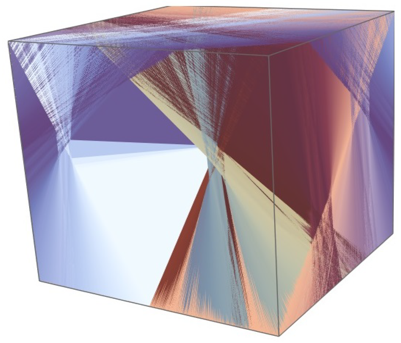
Figure 3 represents the attractor of a dual RPIFS corresponding to the RPIFS given in [10] (Section 4, Example 4.0.1, with scaling factor $d=0.3$).

Conjecture 1. 

If G is the graph of the RPFIF corresponding to the RPIFS $\mathcal{W}=\left\{{\mathbb{RP}}^2\setminus {\mathbb{H}}_{e_3};W_n:n=1,2,\dots ,N\right\}$ given by (8), then there exists an attractor $\widehat{G}$ corresponding to the dual RPIFS $\widehat{\mathcal{W}}=\left\{\widehat{{\mathbb{RP}}^2\setminus {\mathbb{H}}_{e_3}};{\widehat{W}}_n:n=1,2,\dots ,N\right\}$ such that $\widehat{G}$ is also the graph of a self-referential function. Moreover, $\widehat{G}=\left\{p^{\perp }:p\in G\right\}$.

4. Conclusions

In this article, we estimated the fractal dimension of the graph of a RPFIF on the real projective plane which has a linear structure. Since the graph of the RPFIF can be viewed as a subset of ${\mathbb{RP}}^2$ as well as a subset of ${\mathbb{R}}^3$, we calculated the dimensions for both the cases. Finally, we designed an IFS on the dual of the real projective plane ${\mathbb{RP}}^2\setminus {\mathbb{H}}_{e_3}$ and posed an open problem.

The perspective view is the two-dimensional replica of a three-dimensional object in the real world, where the apparent size of an object decreases as its distance from the viewer point increases. The lenses of the camera and the human eye work in the same way, and therefore, the perspective view looks most realistic [20]. In the future direction, one may look into the graph of an RPFIF in a different perspective view and estimated the fractal dimensions of the corresponding images which are made by intersecting the graph of the RPFIF with the object planes/image planes.