Article

A New Perspective on Predicting Roughness of Discontinuity from Fractal Dimension D of Outcrops

1
School of Civil Engineering, Southeast University, Nanjing 211189, China
2
Department of Geotechnical Engineering, College of Civil Engineering, Tongji University, Shanghai 200092, China
*
Author to whom correspondence should be addressed.
Fractal Fract. 2023, 7(7), 496; https://doi.org/10.3390/fractalfract7070496
Submission received: 30 May 2023 / Revised: 17 June 2023 / Accepted: 18 June 2023 / Published: 22 June 2023
(This article belongs to the Special Issue Fractal Analysis and Its Applications in Geophysical Science)

Abstract

:
In tunnel construction, predicting the roughness of discontinuity is significant for preventing the collapse of the excavation face. However, currently, we are unable to use a parameter with invariant properties to quantify and predict the roughness of discontinuity. Fractal dimension D is one such parameter that be used to characterize the roughness of discontinuity. The study proposes a new method to predict the roughness of discontinuity from the fractal dimension D of outcrops. The measurement method of the coordinates of outcrops is firstly summarized, and the most suitable method of calculating fractal dimension D is then provided. For characterizing the spatial variability of fractal dimension D, the random field of fractal dimension D is discretized, and the prediction model is then established based on Bayesian theory. The proposed method is applied to one tunnel for predicting the roughness of discontinuity, and the results indicate that the relative errors of prediction are less than 1.5%. The sensitivities of correlation function and discontinuity size are analyzed. It is found that the different correlation functions have no obvious effect on the prediction results, and the proposed method is well applied to relatively large sizes of discontinuity.

1. Introduction

The properties of the rock masses may be different in different locations of the designed tunnel; this requires the different properties of rock masses to be excavated using different methods, such as NATM (New Austria Tunnelling Method) and TBM (Tunnel Boring Machine) to reduce economic costs and construction time. The existence of discontinuities near the excavation face significantly influences the surrounding rock mass properties; the excavation face could collapse when the properties of the rock mass are poor, presenting the possibility of serious casualties and property damage. The roughness of discontinuity is an important parameter in rock mass classification standards [1,2] and thus its evaluation is important. In recent years, many researchers have studied the roughness of discontinuity [3,4,5,6,7,8]; the prerequisite of such studies is that the discontinuities can be determined. Unfortunately, discontinuities are invisible, except for the discontinuity information exposed on the excavation face; thus, predicting the roughness of discontinuities with the available data is essential.
Because 2D traces are visible on the excavation face, some researchers have proposed using 2D traces on the excavation face to predict the roughness of discontinuity [9]. In tunnel construction, 3D narrow slices (i.e., outcrops), which are the exposed sections of the discontinuities on the excavation face, can be directly observed [10,11]. This can reflect the 3D characteristics of the discontinuity. Based on this, Wang et al. [12] used the slices to predict the roughness of discontinuity and proposed the concept of the required minimum number (RMN) of slices, with the consideration of the difficulty in acquiring such slices in engineering. For calculating the roughness of slices, 3D statistical parameters θs, Rs, and Z2s, which can be used to depict the inclination and size of the asperities, are adopted [12]. However, the values of 3D statistical parameters depend on the sampling interval, which is not a desirable feature for quantifying the roughness [13]. Fractal dimension D is one of the main methods for quantitative description of the roughness of complex surfaces with self-similarity, such as discontinuity; as the roughness of discontinuity changes, the fractal dimension D also changed accordingly. More importantly, fractal dimension D has scale-invariant properties for a range of scales [13].
A new method is provided to predict the roughness of discontinuity from the fractal dimension D of the outcrops, taking into account the difficulty of data acquisition during tunnel construction. The measurement method of outcrops in engineering is firstly summarized, and a comparison of the calculation methods of fractal dimension D is made in order to select the most suitable one. For characterizing the spatial variability of the fractal dimension D, the random field of the fractal dimension D is discretized. The prediction model is then established according to Zhang et al. [9]. The proposed method is applied to tunnel engineering for predicting the roughness of the discontinuity. Finally, the sensitivities of the correlation function and the discontinuity size are analyzed with regard to the prediction results.

2. Measurement of Fractal Dimension D of Outcrops

In tunnel construction, outcrops are visible on the excavation face; it is necessary to extract the coordinates of the outcrops to characterize the roughness of the outcrops. In this section, the coordinates of the outcrops are measured using 3D laser scanning, and the most suitable method of calculating the fractal dimension D is determined by comparison.

2.1. Measurement of Coordinates of Outcrops

The coordinates of outcrops can be obtained from a point cloud model, which can be constructed using 3D laser scanning [11]. 3D laser scanning is a non-contact measuring technique that can be used to scan the excavation face and obtain the coordinates of the point cloud of the excavation face [14,15]. It is widely used in the field of tunnel construction; see Figure 1a. In the study, the distance measurement accuracy of the 3D laser scanner could reach 1 mm, and the distance measurement radius was 150 m, which satisfies the requirements for accuracy in tunnel construction. The host was equipped with a high-definition HDR color camera with up to 165 million pixels, and clear images could be easily obtained. For obtaining complete coordinates of outcrops, it is necessary to scan the excavation face from different positions, and images from different positions should be combined using artificial tie-points to ensure the accuracy of the integrated image [10].
The point cloud model can be then constructed, as shown in Figure 1b, but it could not be used to directly extract the coordinates of outcrops [10]. The following steps were taken to realize point cloud data processing: (1) coordinate transformation of the point cloud data; (2) registration of the point cloud data; (3) non-surface data filtering; (4) establishment of a surface triangular mesh model [10,11].
The outcrops can be identified by the method proposed by Cao et al. [10]; they are geometrically recognized as sharp edges of adjacent planes with large angles. For eliminating the noises produced by the algorithm, several steps can be adopted, as outlined in [10]. The coordinates of all outcrops can be then obtained, as shown in Figure 1c.

2.2. Calculation Method of Fractal Dimension D

Fractal geometry theory was initially proposed by Mandelbrot for addressing extremely irregular phenomena in the nature [16,17]; geologists then used the theory to study the roughness of discontinuity. The triangular prism surface area method [18], projective covering method [19,20], and cubic covering method [21,22,23,24] are the main methods used to depict the fractal characteristic of discontinuity, as shown in Figure 2.
For the triangular prism surface area method, the core of the method involves calculating the surface area of the triangular prism. The surface abcd is composed of four triangulars, and the surface area of abcd equals the sum of the surface area of aob, boc, doa, and doc, as shown in Figure 2a. However, the midpoint o of abcd may not necessarily be on the outcrop surface, so the surface area of the triangular prism may not be accurate. In Figure 2c, the cubic covering method uses cubes with length t covering rough surfaces, and the box-counting dimension can be calculated by calculating the quantity of cubes that can completely cover the surface of the discontinuity [23]. However, this method has difficulty distinguishing I and II in Figure 2d. It can be found that the quantities of the cubes of I and II are all equal to 2, but the roughness of I and II are obviously different.
The projective covering method is shown in Figure 2b, and the fractal dimension D calculated by the method ranges from 2 to 3. Equation (1) can be used to calculate the total surface area of the discontinuity. Glynn proposed the modified projective covering method [25]; the fractal dimension D of the discontinuity can be calculated using Equation (2). The method avoids the disadvantage of the triangular prism surface area method and cubic covering method. The calculation of the surface area of abcd is more accurate than that of the triangular prism surface area method, as expressed by Equation (1). The surface areas of III and IV can be well distinguished in Figure 2d.
S = 1 2 { [ t 2 + ( h 4 h 1 ) 2 ] 1 2 [ t 2 + ( h 2 h 1 ) 2 ] 1 2 + [ t 2 + ( h 4 h 3 ) 2 ] 1 2 [ t 2 + ( h 3 h 2 ) 2 ] 1 2 }
S = 1 2 t [ t 2 + ( h 4 h 1 ) 2 + ( h 2 h 1 ) 2 + t 2 + ( h 4 h 3 ) 2 + ( h 3 h 2 ) 2 ]
D = 2 K
where t is the side length of the discrete square; h1, h2, h3, and h4 are the discrete point (a, b, c, and d) heights of point clouds, respectively; K is the slope of the total surface area of the discontinuity (STotal) against the scale of the cube (t) in log-log scale coordinates system.

3. Prediction of Fractal Dimension D of Discontinuity

For predicting the fractal dimension D of the discontinuity in the tunnel construction, it is essential to consider the difficulty of the data acquisition during the tunnel construction. The geotechnical parameters, which are in different positions in the same space, often present randomness and relevance, which are essential for reducing the sample quantity [7]. Therefore, the discretization of the random field of the fractal dimension D is conducted for calculating the statistical parameters μ, σ, and λ. The fractal dimension D of the discontinuity is then predicted based on this.

3.1. Discretization of Random Field of Fractal Dimension D

Rock properties are variable over space, as they exist in natural states and can be restructured as a result of depositional, post-depositional or weathering processes [26,27]. It is necessary to investigate the spatial variability of the outcrops for predicting the fractal dimensional D of the discontinuity; the random field is used to characterize the spatial variability [28]. The random field can be characterized by the three parameters μ, σ, and λ. Among them, μ and σ are the average and standard deviation of the fractal dimension D of the outcrop samples; they reflect concentration trend and dispersion degree of fractal dimension D samples, respectively. The fractal dimension D between different locations exhibits correlation, as shown in Figure 3, and λ can describe the spatial correlation degree of the fractal dimension D of the outcrop samples. For characterizing the spatial variability of the fractal dimension D, it is necessary to discretize the random field [29,30]. In the study, the discretized random field is established by using the fractal dimension D to characterize the outcrops with the width of t mm in the engineering. μ, σ, and λ can be calculated from the point coordinates in Figure 3. Correlation function ρ(τ) can be then used to describe the variability of the fractal dimension D of the outcrops. Zhang et al. [9] considered that the correlation function exerts no influence on the prediction results of JRC3d, and single exponential correlation function (SECF) is chosen as the most probable correlation function in depicting the spatial variability of JRC2d. The sensitivity of the correlation function in the prediction results is analyzed in Section 4.

3.2. Establishment of Prediction Model of Fractal Dimension D

Zhang et al. [9] proposed predicting the JRC3d of the discontinuity based on traces. The trace samples of the discontinuity under study and the prior information (μ, σ, and λ) collected from the existing discontinuities were fully utilized. The JRC3d prediction model is established by combining the trace samples with the prior information in accordance with Bayesian theory. The current study predicts the fractal dimension D from the outcrop samples, using the same scenario as the model proposed by Zhang et al. [9]; thus, the prediction model can be updated as Equations (4)–(7), which can be used to predict the fractal dimension D of the discontinuity. Equation (4) results in the mean μ0 corresponding to the maximum probability of the posterior distribution of μ (i.e., Equation (5)) predicting the fractal dimension D of discontinuity. Equations (6) and (7) are combined with Equation (5) to update the parameters σ, and λ. It can be found that the equation is established based on the fact that the average of fractal dimension D of the outcrops is approximately equal to the fractal dimension D of the whole discontinuity; whether the above conclusion is sensible should be further validated.
D = A r g max μ [ P ( μ σ , λ , ξ ^ _ ) ]
P ( μ σ , λ , ξ ^ _ ) P ( ξ ^ _ μ , σ , λ ) P ( μ )
P ( σ μ , λ , ξ ^ _ ) P ( ξ ^ _ μ , σ , λ ) P ( σ )
P ( λ μ , σ , ξ _ ^ ) P ( ξ _ ^ μ , σ , λ ) P ( λ )
where  ξ ^ _  is the vector composed of samples of the fractal dimension D acquired from outcrops;  P ( ξ _ ^ μ , σ , λ )  is the likelihood function of μ, σ, and λ; P(μ), P(σ), and P(λ) are the prior distributions of μ, σ, and λ respectively.
For validating the effectiveness of the above conclusion, the study collected one complete discontinuity from one tunnel using 3D laser scanning; the discontinuity sample is the same as the discontinuity to be used for verifying the proposed method in Section 4. In the study process, the discontinuity is divided into n parts, and each part is assumed to represent one outcrop. The width of the outcrops is initially set as 5 mm to calculate the average of the fractal dimension D of the outcrops, as shown in Figure 4a. The fractal dimension D of each outcrop and the whole discontinuity are calculated using Equations (1) and (2). The fractal dimension D of each outcrop changes from 2.074 to 2.079, and the fractal dimension D of the whole discontinuity is equal to 2.015. It can be found that the average of the fractal dimension D of the outcrops (i.e., 2.076) is bigger than that of the discontinuity (i.e., 2.015). For studying whether the relationship always exists in the discontinuity, the widths of the outcrop are likewise set to 2 mm, 4 mm, 6 mm, 8 mm, and 10 mm. The calculation results of the fractal dimension D of the outcrops are shown in Figure 4b–f.
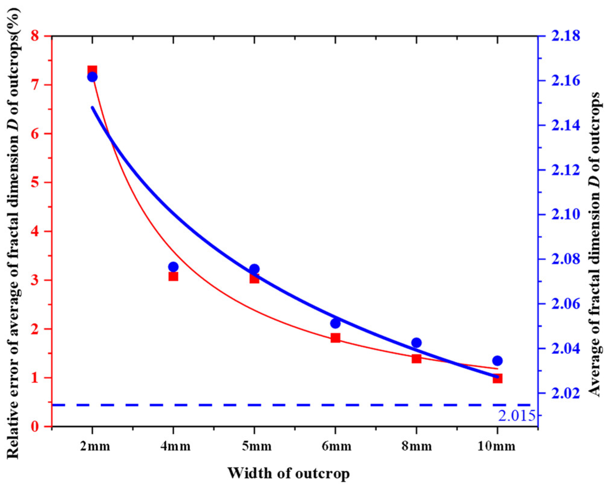
It can be easily found that the fractal dimension D of the outcrops is bigger than that of the discontinuity; however, the fractal dimension D of the outcrops approaches that of the discontinuity, and the trend gradually becomes slower with the larger width of the outcrop, as shown in Figure 5. Therefore, the average of the fractal dimension D of the outcrops is not completely equal to the fractal dimension D of the whole discontinuity, whether the width is set as 2 mm, 4 mm, 6 mm, 8 mm or 10 mm, but the values are closer with the larger width of the outcrop.
For adopting the model established by Zhang et al. [9], it is necessary to make the error standard for selecting the most appropriate width to predict the fractal dimension D of the discontinuity. The relative error is generally used to evaluate the credibility of the prediction result; it is calculated by Equation (8).
Relative   error ( % ) = Average   of   fractal   dimension   D   of   outcrops     Fractal   dimension   D   of   discontinuity Fractal   dimension   D   of   discontinuity × 100 %
The relative errors of the average of the fractal dimension D of the outcrops with the width of 2 mm, 4 mm, 5 mm, 6 mm, 8 mm, and 10 mm are 7.30%, 3.07%, 3.03%, 1.82%, 1.39%, and 0.99%, respectively, as shown in Figure 5. It can be found that the difference between the widths of 2 mm and 4 mm is more than 4%, but the difference between the widths of 4 mm and 10 mm is approximately 2%. Considering the trade-off between the width of the outcrop and the relative error, the width of 4 mm is sufficient to use Equations (4)–(7) to predict the fractal dimension D of the discontinuity.
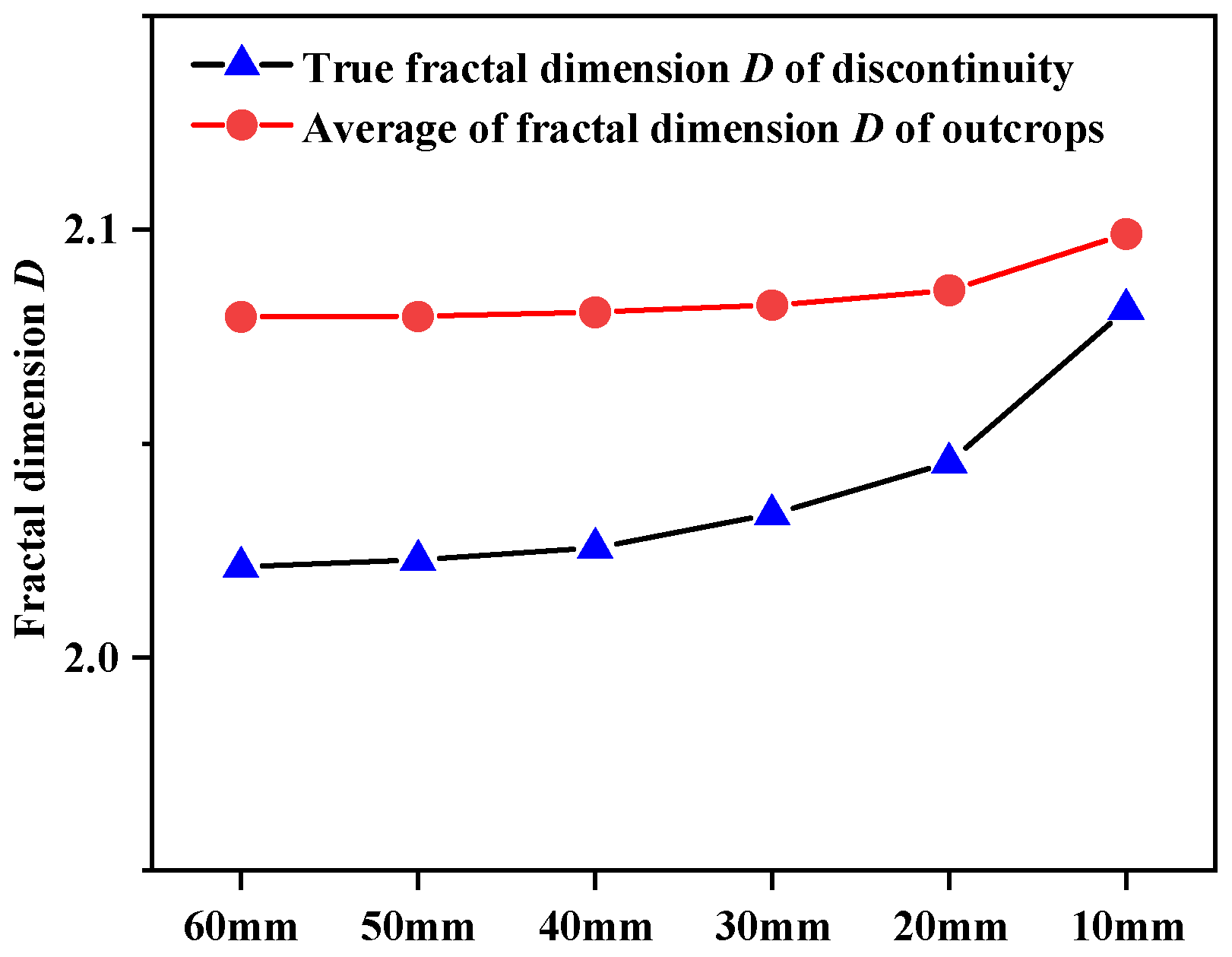
More discontinuity samples are used to verify the conclusion in Figure 6. It can be easily found that true fractal dimension D of the discontinuity has a similar change amplitude to the average of the fractal dimension D of the outcrops, which further validates that there is a strong correlation between true fractal dimension D of the discontinuity and the average of the fractal dimension D of the outcrops. Therefore, it also further validates the effectiveness of Equation (4).
Multidimensional Gaussian distribution can be used to express the likelihood function [9,31,32], as follows:
P ( ξ ^ _ μ , σ , λ ) = ( 2 π σ 2 ) M / 2 det R 1 / 2 × exp [ 1 2 σ 2 ( ξ ^ _ μ l _ ) T R _ 1 ( ξ ^ _ μ l _ ) ]
where
R = ρ 11 ρ 12 ρ 1 M ρ 21 ρ 22 ρ 2 M ρ M 1 ρ M 2 ρ M M
where M is the number of samples of the fractal dimension D l ¯  is a unit vector of M rows and one column;  ρ m  is the correlation function of fractal dimension D; R is the correlation function matrix.
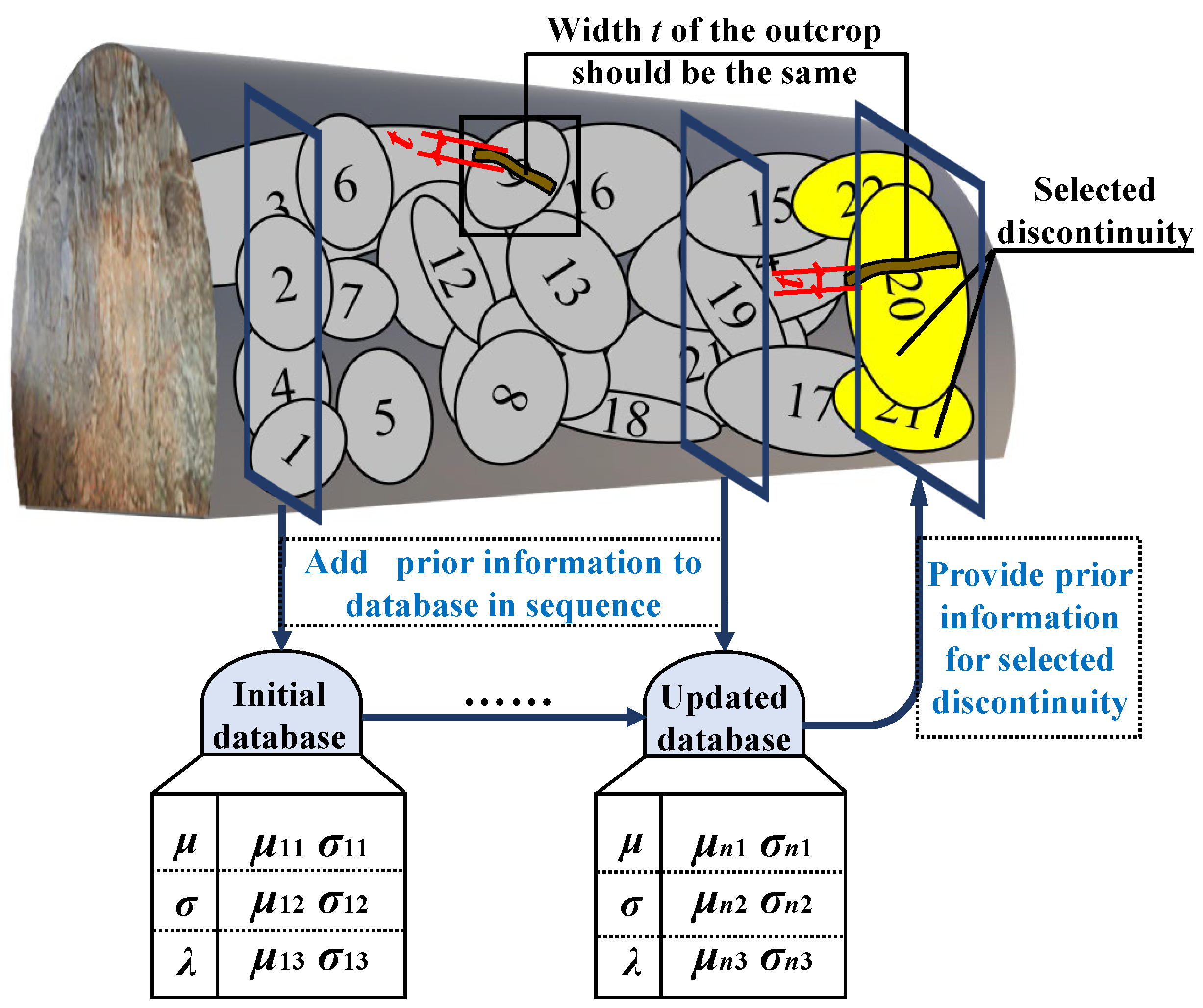
Considering the characteristics of the semi-enclosed spaces of the tunnels, the prior distributions could be dynamically determined by Bayesian updating [33,34,35,36,37,38,39]. The prior data of μ, σ, and λ are constantly added to the database with the tunnel excavation, as shown in Figure 7. Considering the application convenience of prior distributions, the normal or lognormal distributions can be used to fit the prior data, and statistical parameters (i.e., μk1, σk1, μk2, σk2, μk3, and σk3, where k represents the kth database update, μk1 and σk1 are the mean and standard deviation of μ, μk2 and σk2 are the mean and standard deviation of σ, and μk3 and σk3 are the mean and standard deviation of λ) in the two distribution types should be determined dynamically. The prior distributions, P(μ), P(σ), and P(λ), can then be derived. It should be noted that the width t of the outcrops of the excavated discontinuities should be coincident with that of the discontinuity to be studied due to the discretization of the random field of the fractal dimension D, as shown in Figure 7.
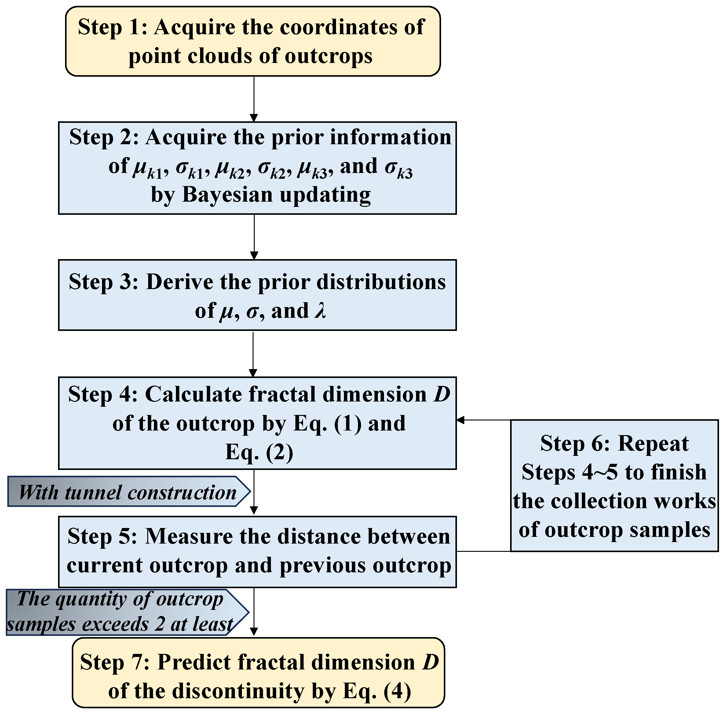
It can be easily found that the posterior distribution  P ( ξ ^ _ μ , σ , λ ) P ( μ )  is complex, so it is difficult to calculate the result of the posterior distribution directly. The Markov chain Monte Carlo (MCMC) sampling method can solve the complex integral problem. The study adopts the hybrid MCMC algorithm; refer to [9] for the more details. The implementation procedure of predicting the fractal dimension D of the discontinuity is shown in Figure 8.

4. Verification of Proposed Method and Sensitivity Analysis of Correlation Function and Discontinuity Size in Predicting Results

4.1. Verification of Proposed Method for Discontinuity Sample

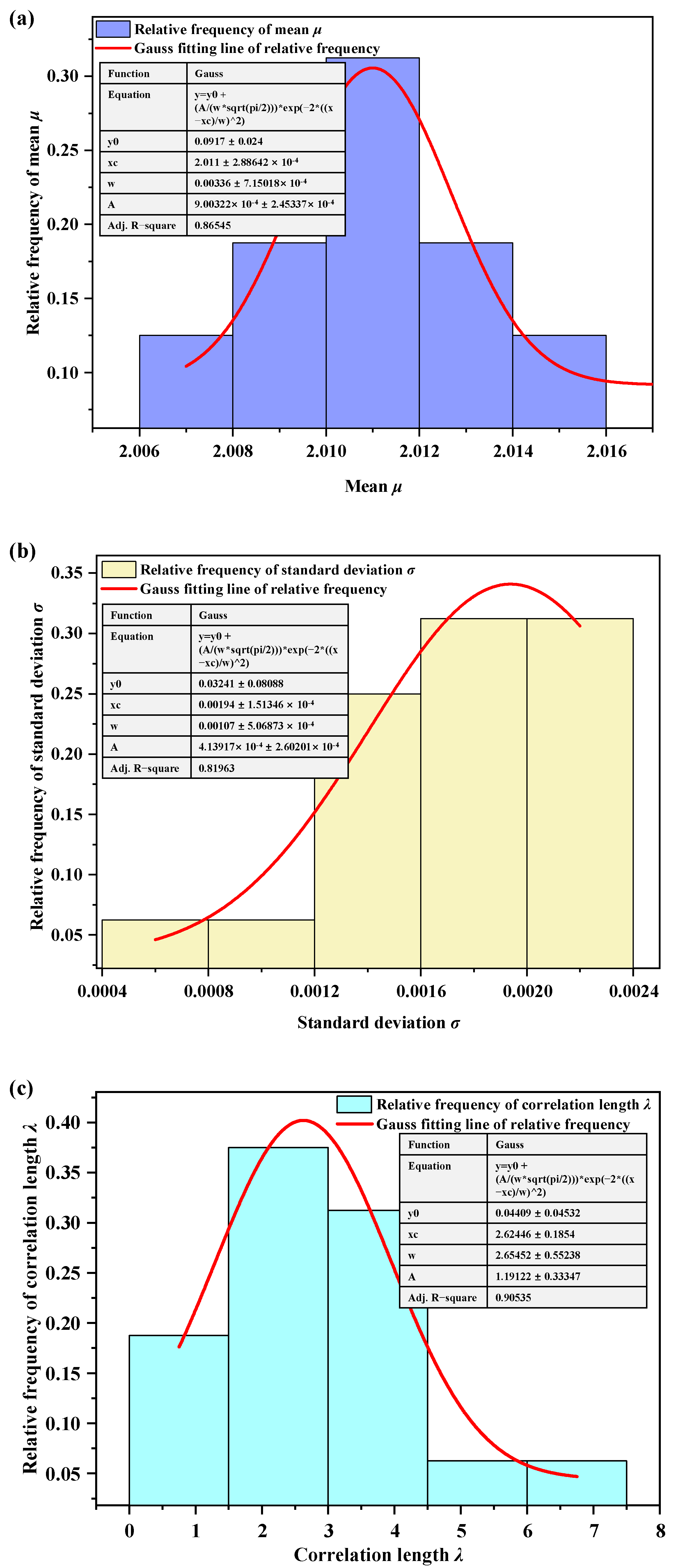
One tunnel is used as the case study, and one discontinuity existing in the tunnel section is used for verifying the proposed method. The following preparations were made before adopting the prediction model. Firstly, the width of 4 mm was determined as the width of the outcrop of the discontinuities. Secondly, SECF (single exponential correlation function) was preliminarily selected as the most probable correlation function. Thirdly, the sample size was set as 2, 3, 4, and 5. Finally, the prior distributions of μ, σ, and λ should be derived by Bayesian updating. For determining the prior distributions, the team conducted in-depth investigation of the site and collected prior data of the discontinuities with 3D laser scanning. With the measurement of the multiple sections, the database was gradually updated. The prior distributions of μ, σ, and λ are shown in Figure 9a–c. The relative frequency of μ, σ, and λ can be fitted by the Gaussian distribution (i.e., normal distribution), and the adjustment R2 of the three distributions of μ, σ, and λ is 0.87, 0.82, and 0.91, respectively.
The sample size is initially set to 2, and 10 random groups are sampled from 16 outcrops. The prediction results are shown in Figure 10a. The relative errors of the prediction results with the sampling size of 2, 3, 4, and 5 are all smaller than 1.5%, which validates the proposed method. It can be found that the prediction results of the fractal dimension D of the discontinuity are stably in the range of [2.03593, 2.03725], and the relative errors of the prediction results are distributed as [1.06, 1.12]. This demonstrates that the prediction accuracy is relatively high when the sampling size is 2. In addition, because the fractal dimension D as calculated by the method ranges from 2 to 3, and the surface of the discontinuity is rougher with the larger fractal dimension D, it can be judged that the surface of discontinuity under study is relatively smooth. In rock mass classification standards, the roughness of discontinuity is one of the influencing factors, and the determination of the roughness of discontinuity is useful to classify the rock mass. GSI (Geological Strength Index) is an important rock mass classification standard [2,40], and the level of the roughness of discontinuity (Rr) can be evaluated as 1.
For deeply investigating whether the quantity of the outcrop samples could affect the prediction accuracy of the fractal dimension D of discontinuity, the quantity of the outcrops is then set to 3, 4, and 5. Ten random groups are also analyzed, and the prediction results are shown in Figure 10a. The prediction results of the fractal dimension D of the discontinuity and the relative errors of the fractal dimension D are marked by four different colors. It is noted that the green lines are straight, and the prediction results with the sampling size of 5 are all equal to 2.012. When analyzing the MCMC algorithm, the value of the likelihood function is equal to 0, because standard deviation σ is too small, which will lead to the value of  exp { 1 / ( 2 σ 2 ) }  approaching 0. Simultaneously, when the sampling size is larger, the value of  [ ξ ^ _ μ l _ ] T R _ 1 [ ξ ^ _ μ l _ ]  is also larger. Hence, standard deviation σ and the sampling size contribute to the smaller value of  exp { 1 / ( 2 σ 2 ) [ ξ ^ _ μ l _ ] T R _ 1 [ ξ ^ _ μ l _ ] } . When the posterior distribution is equal to 0, the new sample is rejected, and the initial sample is retained. Therefore, the prediction results are the same as the prior information (i.e., 2.012). It also can be found that some prediction results with the sampling size of 4 are equal to 2.012; however, this situation does not occur in the prediction results with the sampling size of 2 and 3.
The averages of the relative errors of the prediction results are shown in Figure 10b. It can be found that the average of the relative errors of the fractal dimension D is 0.129058% with the sampling size of 5, which is the smallest among four sampling sizes. The averages of the relative errors of the prediction results with the sampling sizes of 2, 3, and 4 are equal to 1.1%, 1.28%, and 0.54%, respectively. It can be noted that the average of the relative errors of prediction results with the sampling size of 3 is larger than that of the sampling size of 2. This situation is due to the fact that the prediction results will be more affected by the sampling size when a larger sampling size is used. Because the samples are randomly extracted from the fractal dimension D of the outcrop width of 4 mm, the samples are slightly larger than the true fractal dimension D of the discontinuity. Surprisingly, the above analysis proves that the prediction results with the sampling size of 3 will be not more accurate than that of the sampling size of 2. However, the prediction results with the sampling size of 4 and 5 do not follow this conclusion, because the sampling size is so large that the results of the posterior distribution are always equal 0, and no new sample is accepted.
The above research results mainly consist of three parts: (1) The relative errors of the prediction results with the sampling size of 2, 3, 4, and 5 are all smaller than 1.5%, which verifies the proposed method; (2) when the sampling size is relatively large, the prediction value of the fractal dimension D of the discontinuity may be approximately coincident with the prior information; (3) when the sampling size is relatively small, the prediction results with the small sampling size are not necessarily less accurate than those with the large sampling size.

4.2. Study on Sensitivity of Correlation Function in Prediction Results

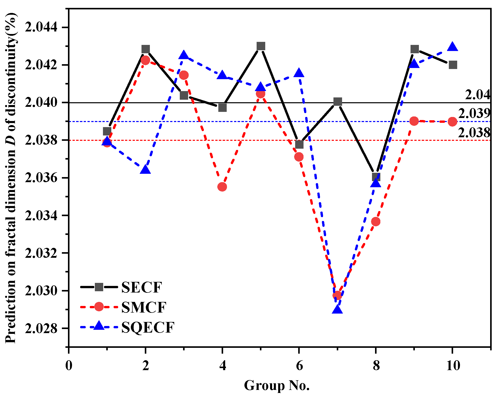
SECF is chosen as the most probable correlation function, and this section will analyze the sensitivity of the correlation functions SECF, SMCF (second-order Markov correlation function), and SQECF (squared exponential correlation function) for the prediction results of the fractal dimension D. The width of the outcrop is 4 mm, and the sampling size is 3. The prediction results are shown in Figure 11. SECF, SMCF, and SQECF are marked by black, red, and blue, and the averages of the predictions results under SECF, SMCF, and SQECF are also denoted by a black line, red line, and blue line. The averages of the prediction results using SECF, SMCF, and SQECF are 2.04, 2.038, and 2.039, respectively. It can be noted that the maximum difference among the three correlation functions is only 0.002%, which validates that the correlation function does not affect the prediction results of the fractal dimension D of the discontinuity.

4.3. Study on Sensitivity of Discontinuity Size in Predicting Fractal Dimension D

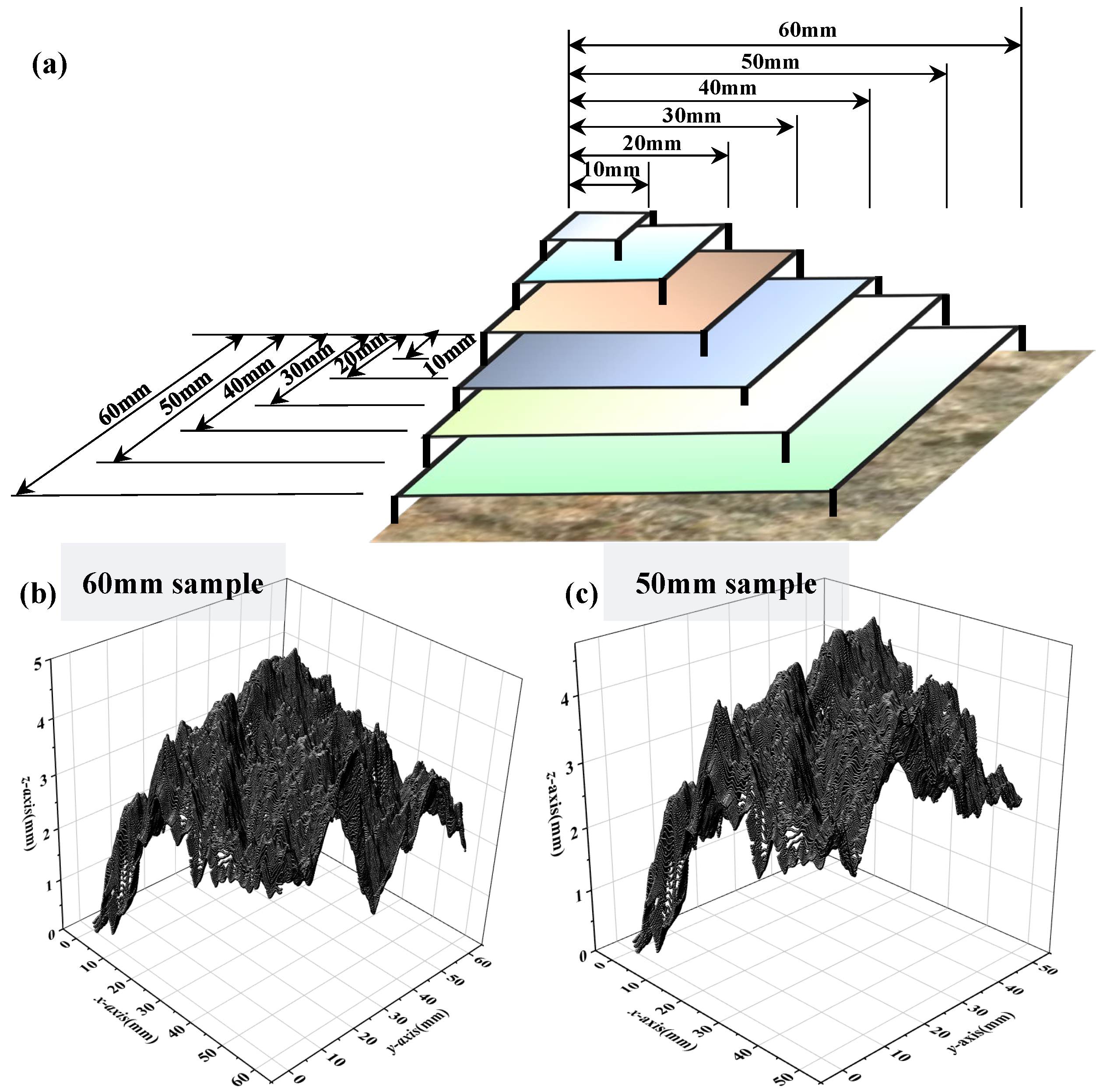
The sizes of the discontinuities are various, so it is essential to study the size effect of the discontinuity. The discontinuity is subdivided into discontinuities with a size of 60 mm, 50 mm, 40 mm, 30 mm, 20 mm, and 10 mm, as shown in Figure 12. The width of the outcrop is still set to 4 mm.
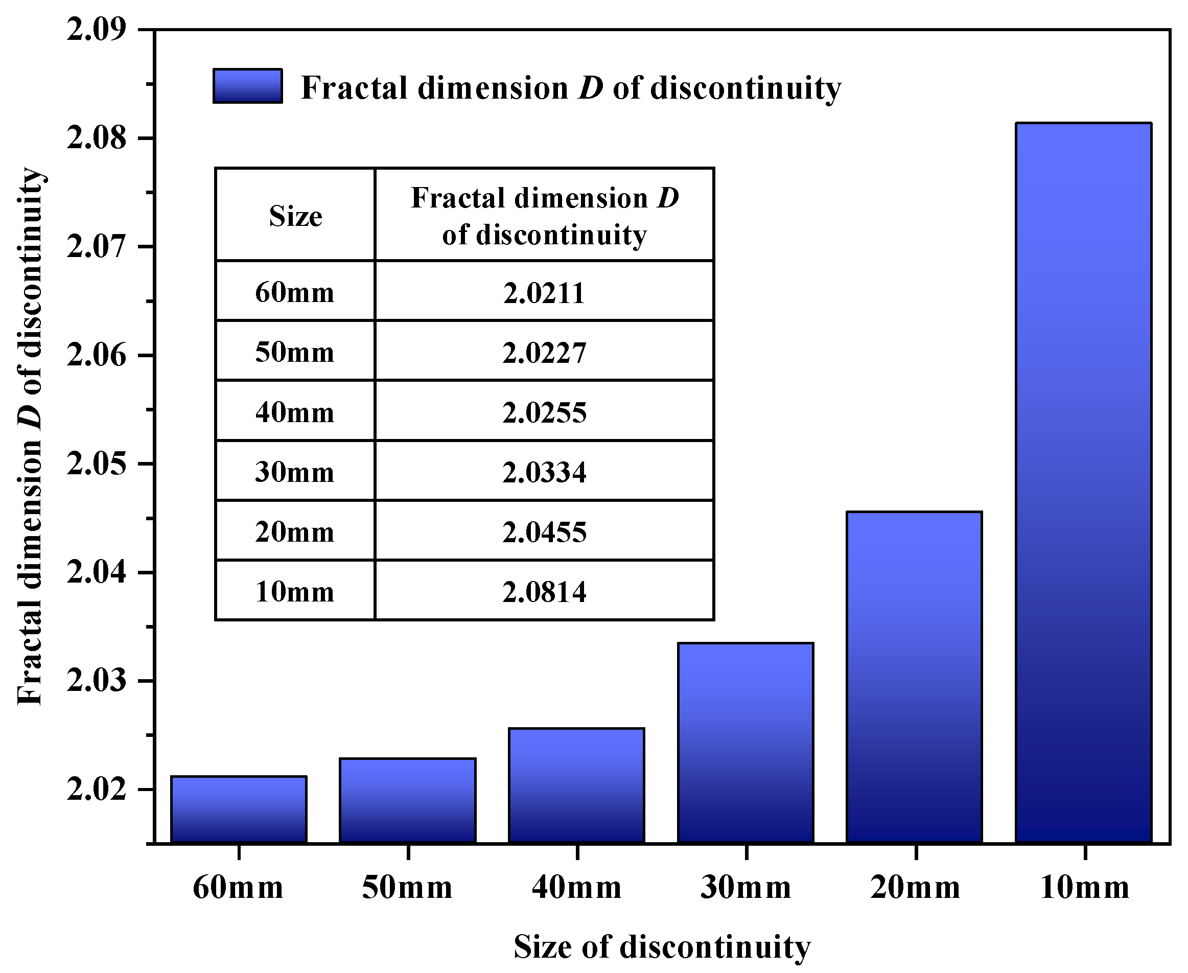
The fractal dimensions D of the discontinuity are shown in Figure 13. The fractal dimension D of the discontinuity with the size of 60 mm, 50 mm, 40 mm, 30 mm, 20 mm, and 10 mm is 2.0211, 2.0227, 2.0255, 2.0334, 2.0455, and 2.0814, respectively. It is noted that the fractal dimension D and its change amplitude is larger with the smaller size of the discontinuity, which is coincident with previous findings.
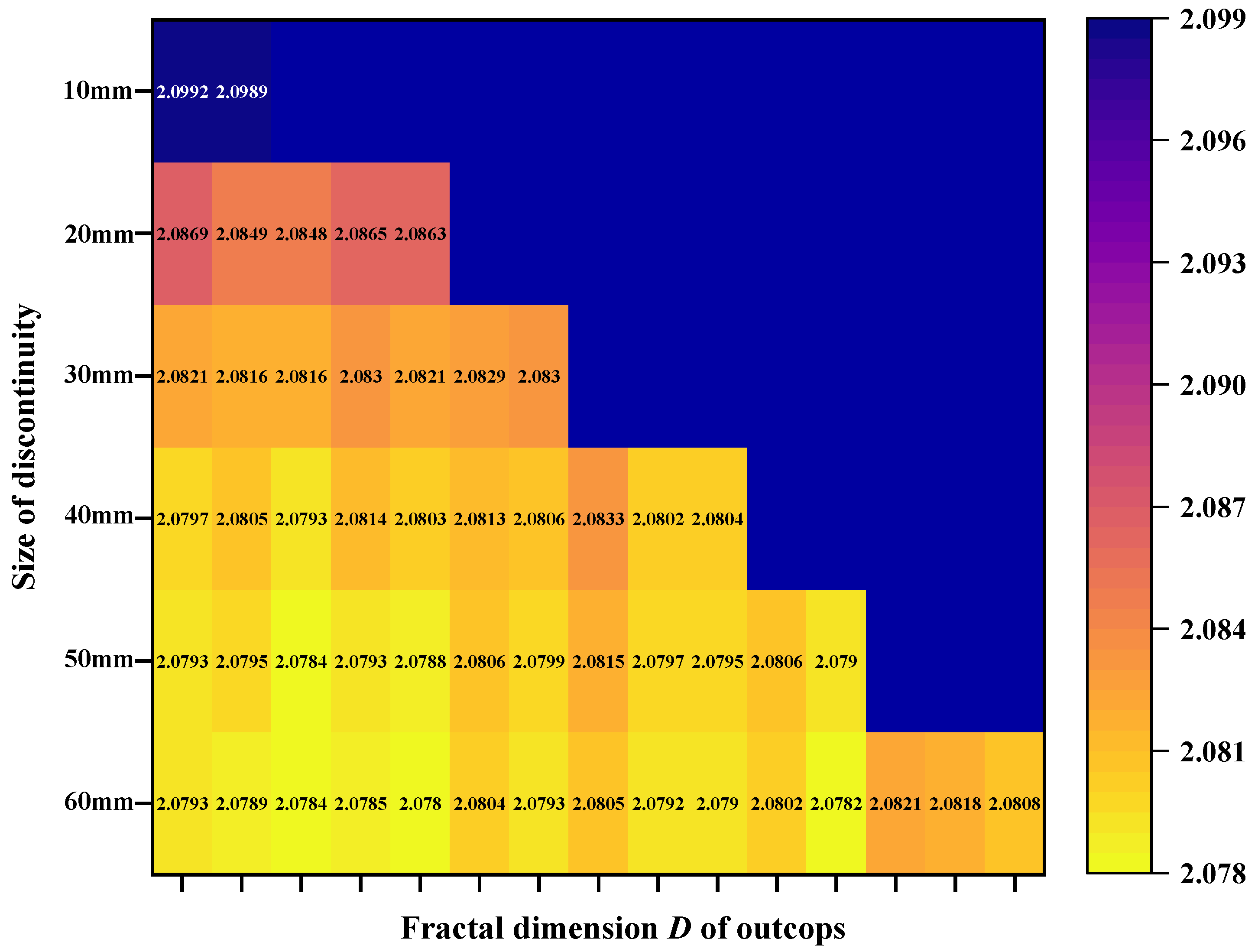
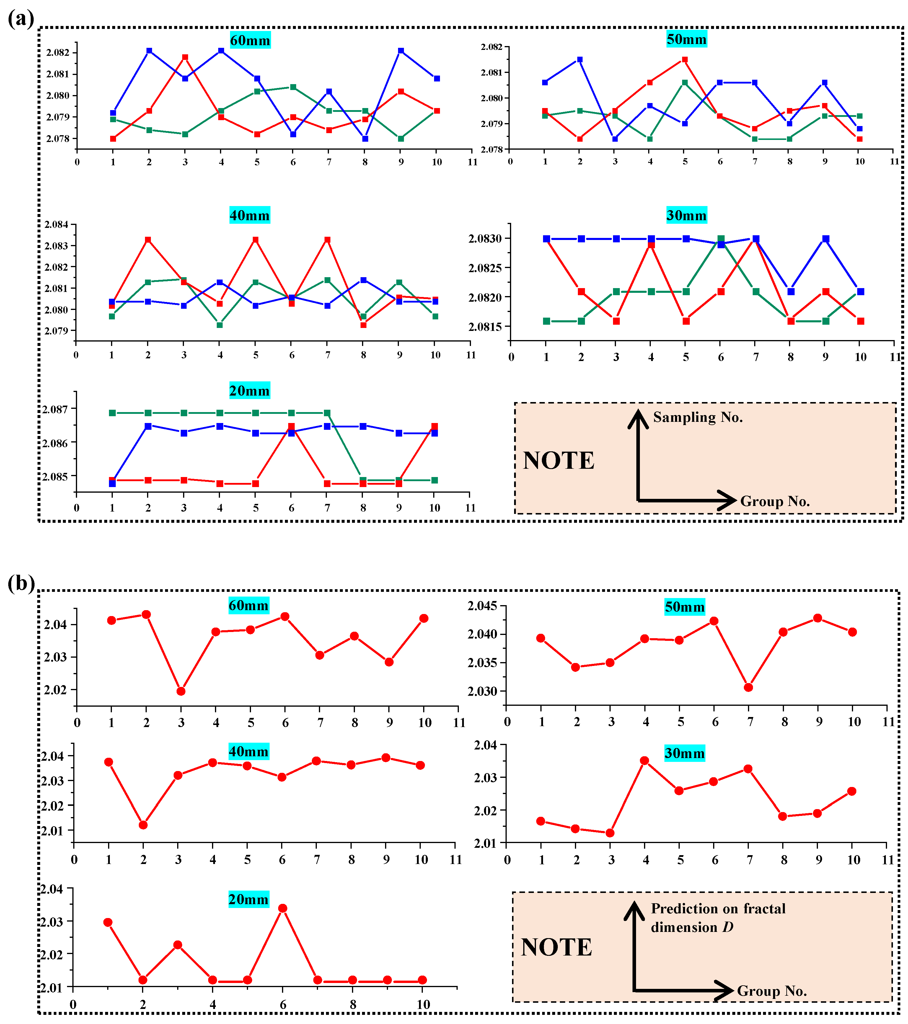
Furthermore, the fractal dimensions D of the outcrops are shown in Figure 14. To obviously distinguish the different fractal dimension D of the outcrops, the results are marked by different colors. It can be found that the fractal dimensions D of the outcrops are also larger as a whole with the smaller size of the discontinuity. The fractal dimensions D of the outcrops of each discontinuity are divided into 10 groups, with the sampling size of 3 for each group using random sampling. The specific group information is shown in Figure 15a, and the discontinuity with the size of 10 mm is ignored as it does not satisfy the sampling requirement. The proposed method is then used to predict the fractal dimension D of the discontinuity, and the prediction results are shown in Figure 15b. The predictions on the fractal dimension D of the discontinuities with the sampling size of 60 mm, 50 mm, 40 mm, and 30 mm have obvious fluctuation trends. On the contrary, the prediction results on the discontinuity with the size of 20 mm are relatively stable, with 70% of prediction values equal to 2.012, which is equal to the previous information on mean μ. As analyzed previously, the values of the corresponding likelihood functions equal 0, which may be owing to the fact that the distances between the samples are short and the differences among the fractal dimensions D of the discontinuities are small. Therefore, the proposed method may be well applied to the relatively large size of the discontinuity but not applied to the small size of the discontinuity, and the distances between the samples should also be considered.
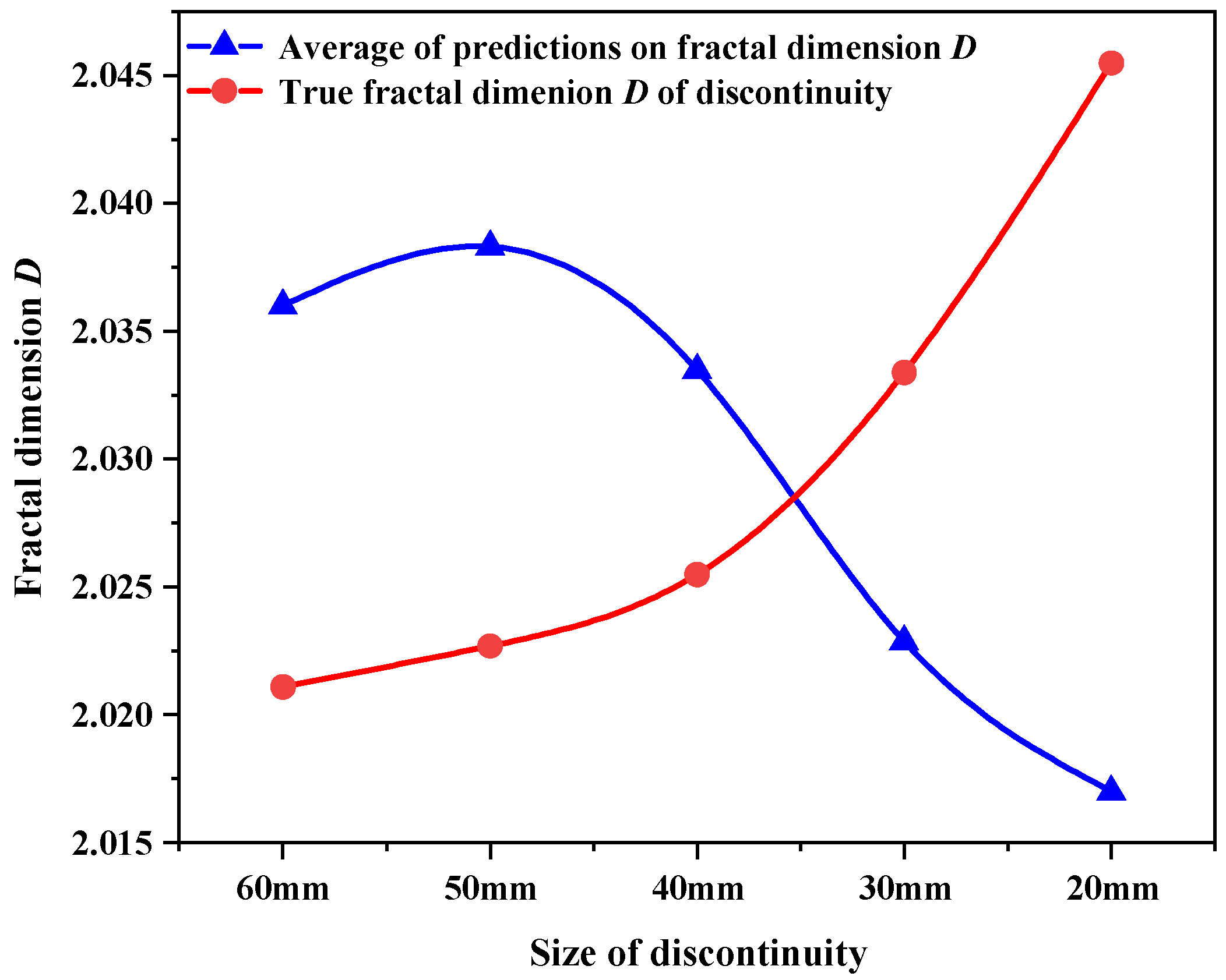
For deeply understanding the effect of the size of discontinuity on the predictions on the fractal dimension D, a comparison between the average of the predictions on the fractal dimension D and true fractal dimension D of the discontinuity is made, which is shown in Figure 16. It can be found that the predictions for the fractal dimension D have a contrary trend to the true fractal dimension D of the discontinuity. More importantly, it is noted that there in an intersection point between two lines in Figure 16 that is useful for predicting the fractal dimension D. For the different discontinuities, the position of the intersection point will change or even not exist, which may be affected simultaneously by the size of the discontinuity, the derivation of the prior information, and the extraction of the random samples.

5. Conclusions

The study proposes a new perspective for the fractal dimension D of the outcrops to predict the fractal dimension D of the discontinuity. The following conclusions can be drawn based on the obtained results:
(1)
For determining the optimal width of the outcrop, the widths of 2 mm, 4 mm, 5 mm, 6 mm, 8 mm, and 10 mm are used for analysis. Considering the trade-off of the between the width of outcrop and the error, the width of 4 mm is selected to conduct follow-up analysis in our case.
(2)
The prediction model of the fractal dimension D is established based on Bayesian theory, according to [9]. For deriving the prior distribution in the model, Bayesian updating is adopted for dynamically determining the prior information of μ, σ, and λ.
(3)
The proposed method is verified by the discontinuity sample, which can be applied to the engineering for predicting the fractal dimension D of the discontinuity. For the GSI standard, the level of the roughness of the discontinuity (Rr) can be evaluated as 1. For choosing the appropriate sampling size in the study, the sampling sizes of 2, 3, 4, and 5 are studied. It is found that when the sampling size is relatively large, the prediction value of fractal dimension D of the discontinuity may be approximately coincident with the prior information. In addition, when the sampling size is relatively small, the prediction results are not necessarily less accurate than those obtained using a large sampling size.
(4)
The sensitivities of the correlation function on the prediction results are analyzed, and the result proves that the correlation function does not affect the prediction results of the fractal dimension D of the discontinuity. The size effect of the discontinuity on the fractal dimension D is analyzed by using discontinuity samples of 10 mm, 20 mm, 30 mm, 40 mm, 50 mm, and 60 mm. The research results indicate that the distances between the samples should also be considered with the application of the method, which means that the proposed method may be well applied to a relatively large size of the discontinuity, but not applied to a small size of the discontinuity.
(5)
There exists an intersection point between two lines represented by the prediction results and the true fractal dimension D, which may be affected simultaneously by the size of the discontinuity, the derivation of the prior information, and the extraction of the random samples. It may be necessary to further study the intersection point for better predicting the fractal dimension D of the discontinuity.

Author Contributions

Conceptualization, Q.Z. and Y.P.; methodology, Y.S.; software, J.L.; validation, Q.Z., Y.S. and M.W.; formal analysis, Y.P.; investigation, Q.Z.; resources, Y.S.; data curation, Q.Z.; writing—original draft preparation, Y.P.; writing—review and editing, X.W.; visualization, J.L.; supervision, X.W.; project administration, Y.P.; funding acquisition, Q.Z. All authors have read and agreed to the published version of the manuscript.

Funding

This research was funded by the National Natural Science Foundation of China, grant numbers 41972277, 42277158, and U1934212.

Data Availability Statement

Not applicable.

Conflicts of Interest

The authors declare no conflict of interest.

References

  1. Bieniawski, Z.T. Engineering classification of jointed rock masses. Trans. S. Afr. Inst. Civ. Eng. 1973, 15, 335–344. [Google Scholar]
  2. Hoek, E.; Brown, E.T. The Hoek-Brown failure criterion and GSI—2018 edition. J. Rock Mech. Geotech. Eng. 2019, 11, 445–463. [Google Scholar] [CrossRef]
  3. Liu, X.G.; Zhu, W.C.; Yu, Q.L.; Chen, S.J.; Li, R.F. Estimation of the joint roughness coefficient of rock joints by consideration of two-order asperity and its application in double-joint shear tests. Eng. Geol. 2017, 220, 243–255. [Google Scholar] [CrossRef] [Green Version]
  4. Diaz, M.; Kim, K.Y.; Yeom, S.; Zhuang, L.; Park, S.; Min, K.B. Surface roughness characterization of open and closed rock joints in deep cores using X-ray computed tomography. Int. J. Rock Mech. Min. Sci. 2017, 98, 10–19. [Google Scholar] [CrossRef]
  5. Cai, Y.; Tang, H.M.; Wang, D.J.; Wen, T. A method for estimating the surface roughness of rock discontinuities. Math. Probl. Eng. 2018, 2018, 9835341. [Google Scholar] [CrossRef]
  6. Magsipoc, E.; Zhao, Q.; Grasselli, G. 2D and 3D roughness characterization. Rock Mech. Rock Eng. 2020, 53, 1495–1519. [Google Scholar] [CrossRef]
  7. Zhang, G.C.; Karakus, M.; Tang, H.M.; Ge, Y.F.; Jiang, Q.Q. Estimation of joint roughness coefficient from three-dimensional discontinuity surface. Rock Mech. Rock Eng. 2017, 50, 2535–2546. [Google Scholar] [CrossRef]
  8. Ban, L.R.; Zhu, C.; Qi, C.Z.; Tao, Z.G. New roughness parameters for 3D roughness of rock joints. Bull. Eng. Geol. Environ. 2019, 78, 4505–4517. [Google Scholar] [CrossRef]
  9. Zhang, Q.; Pei, Y.C.; Wang, X.J.; Li, X.J.; Shen, Y.X. Probabilistic prediction on three-dimensional roughness of discontinuity based on two-dimensional traces under rock tunnel excavation based on Bayesian theory. Undergr. Space, 2023; under review. [Google Scholar]
  10. Cao, T.; Xiao, A.C.; Wu, L.; Mao, L.G. Automatic fracture detection based on terrestrial laser scanning data: A new method and case study. Comput. Geosci. 2017, 106, 209–216. [Google Scholar] [CrossRef]
  11. Pan, D.D.; Li, S.C.; Xu, Z.H.; Zhang, Y.C.; Lin, P.; Li, H.Y. A deterministic-stochastic identification and modelling method of discrete fracture networks using laser scanning: Development and case study. Eng. Geol. 2019, 262, 105310. [Google Scholar] [CrossRef]
  12. Wang, C.; Yong, R.; Luo, Z.; Du, S.; Karakus, M.; Huang, C. A novel method for determining the three-dimensional roughness of rock joints based on profile slices. Rock Mech. Rock Eng. 2023, 56, 4303–4327. [Google Scholar] [CrossRef]
  13. Ge, Y.F.; Kulatilake, P.; Tang, H.M.; Xiong, C.R. Investigation of natural rock joint roughness. Comput. Geotech. 2014, 55, 290–305. [Google Scholar] [CrossRef]
  14. Li, X.J.; Chen, Z.Y.; Chen, J.Q.; Zhu, H.H. Automatic characterization of rock mass discontinuities using 3D point clouds. Eng. Geol. 2019, 259, 105131. [Google Scholar] [CrossRef]
  15. Guo, J.T.; Liu, S.J.; Zhang, P.N.; Wu, L.X.; Zhou, W.H.; Yu, Y.N. Towards semi-automatic rock mass discontinuity orientation and set analysis from 3D point clouds. Comput. Geosci. 2017, 103, 164–172. [Google Scholar] [CrossRef]
  16. Gefen, Y.; Aharony, A.; Mandelbrot, B.B. Phase-transitions on fractals.1. quasilinear lattices. J. Phys. A Math. Gen. 1983, 16, 1267–1278. [Google Scholar] [CrossRef]
  17. Gefen, Y.; Meir, Y.; Mandelbrot, B.B.; Aharony, A. Geometric implementation of hypercubic lattices with noninteger dimensionality by use of low lacunarity fractal lattices. Phys. Rev. Lett. 1983, 50, 145–148. [Google Scholar] [CrossRef]
  18. Clarke, K.C. Computation of the fractal dimension of topographic surfaces using the triangular prism surface-area method. Comput. Geosci. 1986, 12, 713–722. [Google Scholar] [CrossRef]
  19. Xie, H.P.; Wang, J.A.; Stein, E. Direct fractal measurement and multifractal properties of fracture surfaces. Phys. Lett. A 1998, 242, 41–50. [Google Scholar] [CrossRef]
  20. Xie, H.P.; Wang, J.A. Direct fractal measurement of fracture surfaces. Int. J. Solids Struct. 1999, 36, 3073–3084. [Google Scholar] [CrossRef]
  21. Zhou, H.W.; Xie, H. Direct estimation of the fractal dimensions of a fracture surface of rock. Surf. Rev. Lett. 2003, 10, 751–762. [Google Scholar] [CrossRef]
  22. Zhang, Y.; Zhou, H.; Xie, H. Improved cubic covering method for fractal dimensions of a fracture surface of rock. Chin. J. Rock Mech. Eng. 2005, 24, 3192–3196. [Google Scholar]
  23. Ai, T.; Zhang, R.; Zhou, H.W.; Pei, J.L. Box-counting methods to directly estimate the fractal dimension of a rock surface. Appl. Surf. Sci. 2014, 314, 610–621. [Google Scholar] [CrossRef]
  24. Wu, M.Y.; Wang, W.S.; Shi, D.; Song, Z.L.; Li, M.H.; Luo, Y.F. Improved box-counting methods to directly estimate the fractal dimension of a rough surface. Measurement 2021, 177, 109303. [Google Scholar] [CrossRef]
  25. Kwaśny, W. A modification of the method for determination of surface fractal dimension and multifractal analysis. J. Achiev. Mater. Manuf. Eng. 2009, 33, 115–125. [Google Scholar]
  26. Zhu, H.; Zhang, L.M.; Xiao, T.; Li, X.Y. Generation of multivariate cross-correlated geotechnical random fields. Comput. Geotech. 2017, 86, 95–107. [Google Scholar] [CrossRef]
  27. Wang, Q.; Ren, X.D.; Li, J. Modeling of unstable creep failure of spatial variable rocks subjected to sustained loading. Comput. Geotech. 2022, 148, 104847. [Google Scholar] [CrossRef]
  28. Vanmarcke, E.H. Probabilistic modeling of soil profiles. J. Geotech. Eng. Div. 1977, 103, 1227–1246. [Google Scholar] [CrossRef]
  29. Chen, D.F.; Xu, D.P.; Ren, G.F.; Jiang, Q.; Liu, G.F.; Wan, L.P.; Li, N. Simulation of cross-correlated non-Gaussian random fields for layered rock mass mechanical parameters. Comput. Geotech. 2019, 112, 104–119. [Google Scholar] [CrossRef]
  30. Yuan, J.; Papaioannou, I.; Straub, D. Probabilistic failure analysis of infinite slopes under random rainfall processes and spatially variable soil. Georisk 2019, 13, 20–339. [Google Scholar] [CrossRef]
  31. Wang, Y.; Au, S.-K.; Cao, Z. Bayesian approach for probabilistic characterization of sand friction angles. Eng. Geol. 2010, 114, 354–363. [Google Scholar] [CrossRef]
  32. Wang, Y.; Cao, Z. Probabilistic characterization of young’s modulus of soil using equivalent samples. Eng. Geol. 2013, 159, 106–118. [Google Scholar] [CrossRef]
  33. Papaioannou, I.; Straub, D. Reliability updating in geotechnical engineering including spatial variability of soil. Comput. Geotech. 2012, 42, 44–51. [Google Scholar] [CrossRef] [Green Version]
  34. Targoutzidis, A. A Monte Carlo simulation for the assessment of Bayesian updating in dynamic systems. Reliab. Eng. Syst. Saf. 2012, 100, 125–132. [Google Scholar] [CrossRef]
  35. Straub, D.; Papaioannou, I. Bayesian updating with structural reliability methods. J. Eng. Mech. 2015, 141, 04014134. [Google Scholar] [CrossRef] [Green Version]
  36. Huang, J.S.; Zeng, C.; Kelly, R. Back analysis of settlement of teven road trial embankment using Bayesian updating. Georisk 2019, 13, 320–325. [Google Scholar] [CrossRef]
  37. Rahimi, M.; Shafieezadeh, A.; Wood, D.; Kubatko, E.J.; Dormady, N.C. Bayesian calibration of multi-response systems via multivariate Kriging: Methodology and geological and geotechnical case studies. Eng. Geol. 2019, 260, 105248. [Google Scholar] [CrossRef]
  38. Hu, B.A.; Gong, Q.M.; Zhang, Y.Q.; Yin, Y.H.; Chen, W.J. Characterizing uncertainty in geotechnical design of energy piles based on Bayesian theorem. Acta Geotech. 2022, 17, 4191–4206. [Google Scholar] [CrossRef]
  39. Tian, H.M.; Cao, Z.J.; Li, D.Q.; Du, W.Q.; Zhang, F.P. Efficient and flexible Bayesian updating of embankment settlement on soft soils based on different monitoring datasets. Acta Geotech. 2022, 17, 1273–1294. [Google Scholar] [CrossRef]
  40. Sönmez, H.; Ulusay, R. A discussion on the Hoek-Brown failure criterion and suggested modifications to the criterion verified by slope stability case studies. Yerbilimleri 2002, 26, 77–99. [Google Scholar]
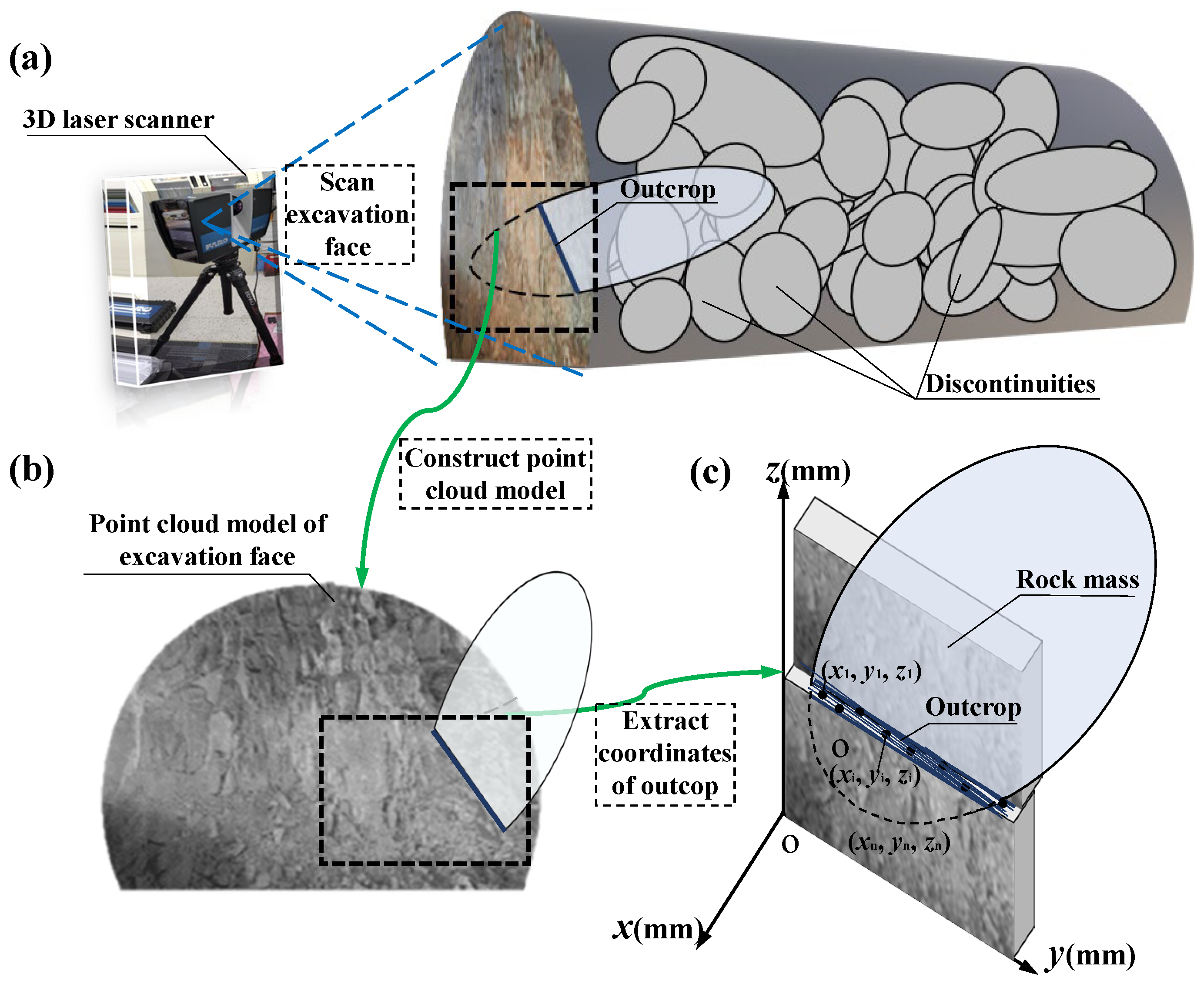
Figure 1. Schematic diagram of extracting the coordinates of the outcrops: (a) scan of the excavation face; (b) establishment of the point cloud model; (c) extraction of the coordinates of outcrops.
Fractalfract 07 00496 g001
Figure 2. Three different methods of calculating the fractal dimension D: (a) triangular prism surface area method; (b) projective covering method; (c) cubic covering method; (d) comparison between the projective covering method and cubic covering method.
Fractalfract 07 00496 g002
Figure 3. Discretization of the random field of the fractal dimension D.
Fractalfract 07 00496 g003
Figure 4. The fractal dimension D of the outcrops with different widths: (a) 5 mm; (b) 2 mm; (c) 4 mm; (d) 6 mm; (e) 8 mm; (f) 10 mm.
Fractalfract 07 00496 g004
Figure 5. Averages of the fractal dimension D of the outcrops and their corresponding relative errors.
Fractalfract 07 00496 g005
Figure 6. Comparison of true fractal dimension D of the discontinuity and the averages of the fractal dimension D of the outcrops.
Fractalfract 07 00496 g006
Figure 7. Schematic diagram of Bayesian updating of μ, σ, and λ.
Fractalfract 07 00496 g007
Figure 8. Implementation procedure of the proposed method.
Fractalfract 07 00496 g008
Figure 9. Prior distributions of (a) μ; (b) σ; (c) λ.
Fractalfract 07 00496 g009
Figure 10. Analysis of the fractal dimension D of the discontinuity with different sampling sizes (2, 3, 4, and 5): (a) predictions of the fractal dimension D of the discontinuity and the relative errors of the prediction results; (b) averages of the relative errors of the prediction results.
Fractalfract 07 00496 g010
Figure 11. Predictions of the fractal dimension D of the discontinuity using the three different correlation functions (SECF, SMCF, and SQECF).
Fractalfract 07 00496 g011
Figure 12. (a) Cutting method of the subdivided discontinuities with the different sizes (60 mm, 50 mm, 40 mm, 30 mm, 20 mm, and 10 mm); (b) Specific diagram of the subdivided discontinuities.
Fractalfract 07 00496 g012aFractalfract 07 00496 g012b
Figure 13. Fractal dimension D of the discontinuities with different sizes (60 mm, 50 mm, 40 mm, 30 mm, 20 mm, and 10 mm).
Fractalfract 07 00496 g013
Figure 14. Fractal dimension D of the outcrops with different sizes of the discontinuity (60 mm, 50 mm, 40 mm, 30 mm, 20 mm, and 10 mm).
Fractalfract 07 00496 g014
Figure 15. (a) Sampling results with different sizes (60 mm, 50 mm, 40 mm, 30 mm, and 20 mm) of the discontinuity; (b) Prediction results on the fractal dimension D of the discontinuity.
Fractalfract 07 00496 g015
Figure 16. Averages of the predictions on the fractal dimension D of the discontinuity and the true fractal dimension D of the discontinuity.
Fractalfract 07 00496 g016
Disclaimer/Publisher’s Note: The statements, opinions and data contained in all publications are solely those of the individual author(s) and contributor(s) and not of MDPI and/or the editor(s). MDPI and/or the editor(s) disclaim responsibility for any injury to people or property resulting from any ideas, methods, instructions or products referred to in the content.