Article

Approximation of Aperiodic Signals Using Non-Integer Harmonic Series: The Generalized NAFASS Approach

by
Raoul R. Nigmatullin
1,
Airat A. Khamzin
2 and
Yangquan Chen
3,*
1
Radioelectronics and Informative Measurements Technics Department, Kazan National Research Technical University Named after A.N. Tupolev, K. Marx Str. 10, 420111 Kazan, Russia
2
Institute of Physics, Kazan Federal University, Kremlevskaya Str. 18, 420008 Kazan, Russia
3
MESA Lab, School of Engineering, University of California, Merced, CA 95343, USA
*
Author to whom correspondence should be addressed.
Fractal Fract. 2023, 7(7), 498; https://doi.org/10.3390/fractalfract7070498
Submission received: 8 May 2023 / Revised: 5 June 2023 / Accepted: 14 June 2023 / Published: 23 June 2023
(This article belongs to the Section Engineering)

Abstract

:
In this paper, the non-orthogonal amplitude-frequency analysis of smoothed signals (NAFASS) method) is used to approximate discrete aperiodic signals from various complex systems with the non-integer harmonic series (NIHS). When approximating by the NIHS, there is a problem in determining the dispersion law for harmonic frequencies. In the original version of the NAFASS approach, the frequency dispersion law was determined from a linear-difference equation. However, many complex systems in nature have frequency distributions that differ from the linear law, which is used in the conventional Fourier analysis of periodic signals. This paper proposes a generalization of the NAFASS method for describing aperiodic signals by the NIHS with a frequency distribution that satisfies a recursive formula, which coincides with the local generalized geometric mean (GGM). The methodology of the generalized NAFASS method is demonstrated using descriptions of financial data (prices for metals) and sound data (sounds of insects) as examples. The results show the effectiveness of the generalized NAFASS approach for describing real-world time data. This discovery allows us to propose a new classification scheme for smoothed and aperiodic signals captured as responses and envelopes from various complex systems.

1. Introduction

Signals recorded from different complex systems are mostly non-periodic. The processing and fitting of non-periodic or aperiodic signals presents a rather difficult problem.
Aperiodic signals can be represented as periodic, but with a period equal to infinity or coinciding with observation time. Therefore, the frequency spectrum of an aperiodic signal is continuous and the integral Fourier transform should be used for its description [1]. However, the problem with using the continuous Fourier transform to describe non-stationary signals is that it is unable to pinpoint the instantaneous time periods where the actual discrete frequency components are. The discrete aperiodic signal fitting issue cannot be resolved by the integral Fourier transform of aperiodic signals; hence, it cannot be used to predict an aperiodic signal outside of the specified time window interval.
The discrete representations of many analog signals play an important role in their processing. They contain relevant information related to the properties of the signals and admit their processing [2]. In the conventional scheme, signals can be presented in the form of Taylor–Maclaurin, Dirichlet, Laurent, Legendre, Padé, Prony, and Fourier series. The classical Fourier series (FS) is a simple and frequently used tool in the signal processing area. However, the FS does not identify both subharmonic and interharmonic components of the given signal and, in many situations, it has serious drawbacks [3,4,5,6].
The proposed method allows the limitations of the Fourier analysis to be overcome. The Fourier analysis is based on time-frequency methods [7] that were used in the last few decades, namely the fractional [8,9,10], short time [11,12,13], windowed FT [14,15], Gabor [16,17,18], wavelet [19,20,21], Hilbert–Huang [22,23,24], and Fourier–Bessel transformations [25,26], and even decomposition over empirical modes [27,28].
At the outset, we should emphasize the fact that all measured data can be classified and divided into three large groups. The first group of data can be determined as quasi-periodic [29,30,31] and, in almost repeatable experiments, they can be fitted by the segments of the Prony series. The second group of data can be classified as quasi-reproducible [32] and, for these types of data, it becomes possible to propose a “universal” fitting function that is derived from a group of similar measurements that are slightly distorted by uncontrollable external factors. This so-called “intermediate” model can be used for the fitting of data of complex systems if the “true fitting function” that follows from some microscopic model is absent. Finally, the third group refers to a large group of irreproducible data (for example, economic, geophysical, acoustic, and technical data) that can be considered as aperiodic data. These types of data are always irreproducible and present the most difficult class of data for fitting and subsequent quantitative analysis.
In [33], the authors proposed a method for describing stationary AP-signals by approximating the description by the finite non-integer harmonics series (NIHS):
y ( t ) S ( t , K ) = A 0 + k = 0 K 1 [ A c k cos ( Ω k t ) + A s k sin ( Ω k t ) ] A 0 + k = 0 K 1 A m d k cos ( Ω k t φ k ) ,   A m d k = A c k 2 + A s k 2 ,   φ k = tan 1 ( A s k A c k )
where the function y(t) represents the given aperiodic signal and S(t, K) is the fitting function. With the extra degree of freedom gained by not imposing restrictions on the frequency values {   Ω k } , the NIHS better approximates the real aperiodic signal in comparison with the conventional FS. In practice, the NIHS can be computed numerically and adopted for forecasting some values located outside the given temporal interval. In [33], the effectiveness of the NIHS method was demonstrated on the processing of real-world time series.
Another attempt to fit a discrete stationary aperiodic signal by a set of harmonic components was realized by one of the authors (R.R.N.) in paper [34]. This method was defined as the nonorthogonal combined Fourier analysis of the smoothed signals (NOCFASS). It was shown that a minor change of the dispersion law for frequencies as Ωk = a·k + b allows the fitting of a wide set of aperiodic signals. Analyzing the drawbacks of the Fourier and wavelet transformations that were considered in paper [35], one can propose linear-difference Equation (2) (below) for calculation and subsequent fit of the desired frequencies that can form a specific “frequency skeleton” of the complex system considered.
The problem we are going to solve in this paper can be formulated as follows. Is it possible to generalize the previous results obtained in the frame of the non-orthogonal amplitude-frequency analysis of smoothed signals (NAFASS) method [35] for systems having the linear-difference equation
Ω k + p = w k + p 1 Ω k + p 1 + w k + p 2 Ω k + p 2 + + w 0 Ω k
and to propagate Equation (2) for a nonlinear case to describe other frequency distributions associated with the analysis of the given aperiodic signal? Here wk+s (s = 0, 1, …, p − 1) is a set of the given constants/weights and the unknown frequencies Ωk,k+1, …, Ωk+p (forming some dispersion law) are derived from the difference Equation (2). The iteration scheme proposed in paper [35] allows the consideration of other possibilities. In particular, we consider some real data that confirm the following recurrence relationship that is formed by a triple of neighboring frequencies
Ω k + 3 = Ω k + 2 w 2 · Ω k + 1 w 1 · Ω k w 0 with s = 0 2 w s = 1
This relationship can be interpreted as the local (p = 3) and generalized (having the normalized weights ws) geometric mean (GGM) for the desired set of frequencies. The justified arguments in favor of selection (3) as a rather general hypothesis will be explained in the final section of this paper.
The paper is divided into the following sections. In Section 2, we discuss the proposed algorithm and potential extensions. We evaluate the suggested approach using the data at hand in Section 3. There are two subsections in Section 3. Economic statistics are taken into account in Section 3.1, while actual acoustic data are covered in Section 3.2. In Section 4, we review the findings and use Bellman’s inequality to explain a peculiarity of the GGM and add a useful fragment for the correct formula describing the case when the signal is less than the corresponding noise, i.e., S(t) < n(t).

2. The Description of the Algorithm and Possible Generalizations

Initially, we apply the iteration Formula (15) described in paper [35] (for conveniences we provide the basic equations tightly associated with this Formula (A5) in the Mathematical Appendix A), for the calculation of the set of the seed/inoculating frequencies. Then, using expressions (A5) and (A6) for d = 0, 1, 2, we obtain the approximate mean expression for the calculated frequency branch:
Ω k 1 3 b = 1 3 Ω k ( b )
Here, Ω k is the averaged branch of frequencies and the frequencies Ω k ( b ) determine the branches that are obtained at the given number (b = 1, 2, 3) of seed/inoculating frequencies obtained with the help of iteration Formula (A5). The criterion for selection of the optimal frequency branch is based on the expression that defines the relative error value:
RelErr ( % ) = min ( stdev [ y ( t ) S ( t , K ) ] mean ( y ( t ) ) ) · 100 % ,
where the function y(t) represents the given aperiodic signal and S(t, K) is the fitting function (1), where the set of the frequencies Ωk (k = 0, 1, 2, …, K − 1) initially coincides with expression (4) and, then, this set is optimized in accordance with expression (5); “stdev” means standard deviation. In the frame of the NAFASS method, we want to solve two problems. The first problem is related to the fitting of the given data expressed in the form (1) for the given aperiodic signal y(t). The second problem is related to the search of the desired fitting function for the optimized set of frequencies Ωk. In the previous paper [35] for this purpose, we considered the linear relationship (2) for p = 1, 2, 3. However, an optimal criterion for the selection of the desired fitting function for the calculated frequency branch was absent. In this paper, we consider the wide set of the fitting functions that are expressed in the following nonlinear form:
Ω k + p s = q = 0 p 1 w q Ω k + q s ,
where the power-law exponent −1 < s ≤ 1 is located in the most probable interval. However, this interval for the nonlinear parameter s is not unique. The values |s| > 1 are also possible. It is important to consider the limiting value s = 0. Taking the limit at s → 0, we obtain from (6):
Ω k + p = lim s 0   ( q = 0 p 1 w q Ω q s ) 1 / s = q = 0 p 1 exp ( w q ln ( Ω q ) ) = q = 0 p 1 Ω q w q , q = 0 p 1 w q = 1
As shown below, this expression is the most interesting and unexpected result that follows from the previously proposed NAFASS method [35]. Here, the parameter p determines the local boundaries of the generalized geometric mean (GGM). For practical calculations, it is necessary to take the minimal value of this parameter and consider the cases p = 2, 3. Expression (3) can be considered as the most probable case. If we consider the solution of the difference Equation (3), it is easy to derive the desired fitting function from the linear-difference equation written relatively for Φk = ln(Ωk). Taking the natural logarithm from (7), we easily obtain the solution for the calculated set of frequencies Ωk (k = 0, 1, 2, …, K − 1):
Φ k + p = q = 0 p 1 w q Φ k + q     Φ k = q = 0 p 1 C q λ q k ,   Ω k = exp ( q = 0 p 1 C q λ q k )   ,   λ p q = 0 p 1 w q λ q = 0 .
Here, the set of the constants Cq are determined by initial conditions, λq are the roots of the characteristic equation. These basic expressions (8) solve the problem related to the solution of Equation (7) at s → 0. We should stress, also, that because of normalization conditions of the weighting factors wq, one of the roots λ always coincides with the unit value, i.e., λ = 1. This root is very important. If we have the difference equation of the type
Ω k + 2 = 2 · Ω k + 1 Ω k   or   Ω k + 1 = 1 2 ( Ω k + 2 + Ω k ) ,
Then, the solution of this simple difference equation corresponds to double degeneration of the root λ = 1 and the desired solution has a form as follows:
Ω k = Ω 0 + ( Ω 1 Ω 0 ) · k
This linear frequency dependence reproduces the well-known F-transform with Ωk = 2πk/T and the linear spectrum used for the NOCFASS method in paper [34].
The complex conjugated roots for λ are also possible. For p = 3, we obtain the solution for Ωk that follows from the recurrence relationship (8):
Ω k F t k = exp ( C 0 + C 1 λ 1 k + C 2 λ 2 k ) ,   λ 1 , 2 = w 2 1 2 ± ( w 2 1 2 ) 2 w 0
The constants C0–2 are determined by initial conditions associated with frequencies Ω0–2. As discussed below, this function Ftk will serve as the basic fitting function for analysis of different data recorded for complex systems and containing the smoothed aperiodic signals. For high-frequency signals (as discussed below), one can take their low-frequency envelopes for analysis. In order to prove that this function is the most probable, we calculated the relative fitting error defined by the expression below:
RelErr ( s ) = min ( stdev [ Ω k s F t k s ] mean | ( Ω k s ) | ) · 100 %
Based on an analysis of available data obtained from the different sources, one can see that the minimum of this expression exists and, in many cases, the minimal value of s has the limit coinciding with the value s = 0. The details for the proposed data treatment procedure are provided separately for the chosen data.

3. Results and Verification on Real Data

What kind of data can be considered as data characterizing the response of a complex system and containing a set of aperiodic signals? We consider the available data as data characterizing a complex system if the specific/microscopic model containing a minimal number of the fitting parameters is absent. In the absence of a specific model, one can use the function (1) for the fitting of an aperiodic signal that initially minimizes expression (5) for the relative error. Simultaneously with this procedure, we should choose the optimal frequency spectrum Ωk that is derived from expression (12), minimizing the value of the nonlinear power-law exponent s. After derivation of the minimal value of s from (12) and initial selection of the minimal value of the parameter p = 2, 3 associated with boundary limits, one can solve two fitting problems: (1) the optimal fit of an aperiodic signal y(t) and (2) the selection of the fitting function for the optimal frequency spectrum Ωk, mentioned above. The NAFASS method implies the fit of the smoothed aperiodic signals. If the initial data are presented in the form of the trendless noise, then the simple integration procedure taken with respect to its mean value suppresses the high frequencies and the integrated data can be fitted by the function (1). In addition, for obtaining the desired smoothed signals, one can apply the reduction procedure to three incident points (R-3IP) [36] and to the procedure of the optimal linear smoothing (POLS) applied successfully in paper [37]. The combination of these two methods (as discussed below for acoustic data) allows to extract the low-frequency envelopes that will be used for fitting purposes by the NAFASS method. If the chosen data have the clearly expressed random trend (for example, economic data), then the NAFASS method can be applied directly. Therefore, it is logical to start from the fit of some economic data that present the interesting example of aperiodic signals.

3.1. The Treatment of Economic Data

From the site http://www.indexmundi.com/commodities/, accessed on 13 June 2023, one can download the distributions of the monthly prices of some important metals such as Al, Cu, Ni, and Pb, which play an essential role in the world economy. The prices cover the 30-year period from July 1992 to June 2022 and contain 12 × 30 = 360 data points. The values of the mean prices for all four metals (Al, Cu, Ni, and Pb) are expressed in US kilodollars per one metric ton. We show the detailed analysis for the first metal Al. Other metals are analyzed in a similar manner and, therefore, their detailed analyses are omitted. In Figure 1, we show the price distribution for Al for the 30-year period covering the interval July 1992–June 2022. All treatment procedures can be divided into some important steps that should be used as key steps for the analysis of random data/aperiodic signals that have the clearly expressed trends.
  • S1. Calculation of the inoculating/seed frequencies forming the corresponding branches Ω k ( d ) that are calculated with respect to iteration Formula (A5) (see Mathematical Appendix A) and have initially d = 1, 2 and 3 inoculating/seed frequencies. We also chose a reasonable value for the limiting frequency ΩK=50 that was sufficient for providing a fit with the calculated value of the relative error from expression (5), not exceeding 6.5%. These frequencies are shown in Figure 2.
  • S2. The next step is the selection of the optimal frequency branch based on expression (5). The results of this procedure are illustrated by Figure 3 and Figure 4. As follows from Figure 4, the averaged frequency branch <Ωk> and the optimal frequency branch Ωk (obtained from criterion (5) and illustrated in Figure 3) cannot coincide with each other. Substitution of the optimal frequency branch Ωk allows the fitting of the initial random function for Al prices. It is obvious that the desired amplitudes from (1) are evaluated by the linear least square method (LLSM). The fit for this Al price distribution, realized in the frame of the hypothesis (1), is presented in Figure 5. Actually, these two steps solve the first problem mentioned above. Together with this fit, we also show the AFR in Figure 6. We should stress, here, that this AFR has different behavior and does not progress to the monotone decreasing of the amplitudes that is expected in the F-transformation and to providing the convergence of the corresponding Fourier series. This becomes sensitive to some parts of the trend that is observed for the initial Al prices analyzed and needs the specific analysis of an experienced expert who works professionally with economic data.
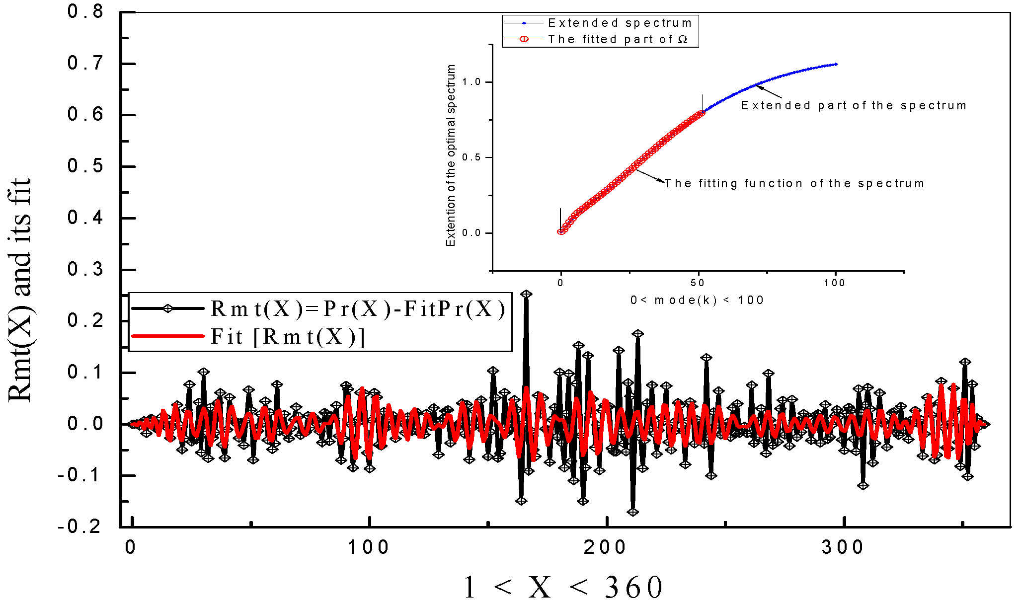
  • S3. To solve the second problem, we formed the function (6) and calculated its relative error for a minimal value of p = 3. We also considered the case p = 2; however, for the same conditions, this case had a large value of the fitting error exceeding 7% and, therefore, we were forced to consider the case p = 3 as the most probable. In the behavior of the relative error, we expected that the case s = 1 would be optimal. This expectation was confirmed by our previous calculations, realized in [30]. However, to our deep amazement, this assumption was not confirmed for all four metals that were subjected to this analysis. The behavior of this function has the clearly expressed minimal value at s = 0, not s = 1! Earlier, for the results presented in paper [30], we did not have this criterion and we analyzed available data in the frame of an approximation corresponding to the linear hypothesis (2) with s = 1. Therefore, this key plot shown in Figure 7 confirms that for the available data analyzed, the hypothesis with s = 0 (expression (3)) that describes the fit of the optimal frequencies is the most real. Figure 7 demonstrates this behavior in detail for the optimal branch of frequencies corresponding to the prices for Al. For the other three metals, a similar behavior for the fitting error related to the function Φk = ln(Ωk) is conserved. The corresponding values of error (0) for all four metals are provided in Table 1. The fit of the optimal frequency with two equivalent functions expressed by relationships (3) and (11) are shown in Figure 8. How do we confirm, in addition, the selection of the chosen hypothesis (3)? The fitting function (11) allows us to increase the frequency range if we extend the initial interval for mode(k) [0, 50] up to the interval [0, 100] and consider the fit of the remnant function that is obtained as the difference between the initial price distribution and its fitting function, provided by expression (1). Additional frequencies help to realize this fit approximately, as shown in Figure 9, with the value of the relative error close to 6%. The AFR for this remnant function confirms, in general, this behavior. With an increasing number of the higher frequencies (q > 50), the behavior of the amplitudes Acq and Asq becomes chaotic. These functions, including their module A m d k = A c k 2 + A s k 2 entering to the AFR, are shown in Figure 10. For the other three metals (Cu, Ni, and Pb), the treatment procedure explained above, in the form of steps S1–S3, is conserved and, therefore, for them we show only the desired fit that is presented in Figure 11. The necessary numeric parameters are also listed in Table 1, Table 2 and Table 3.

3.2. The Treatment of Acoustic Data

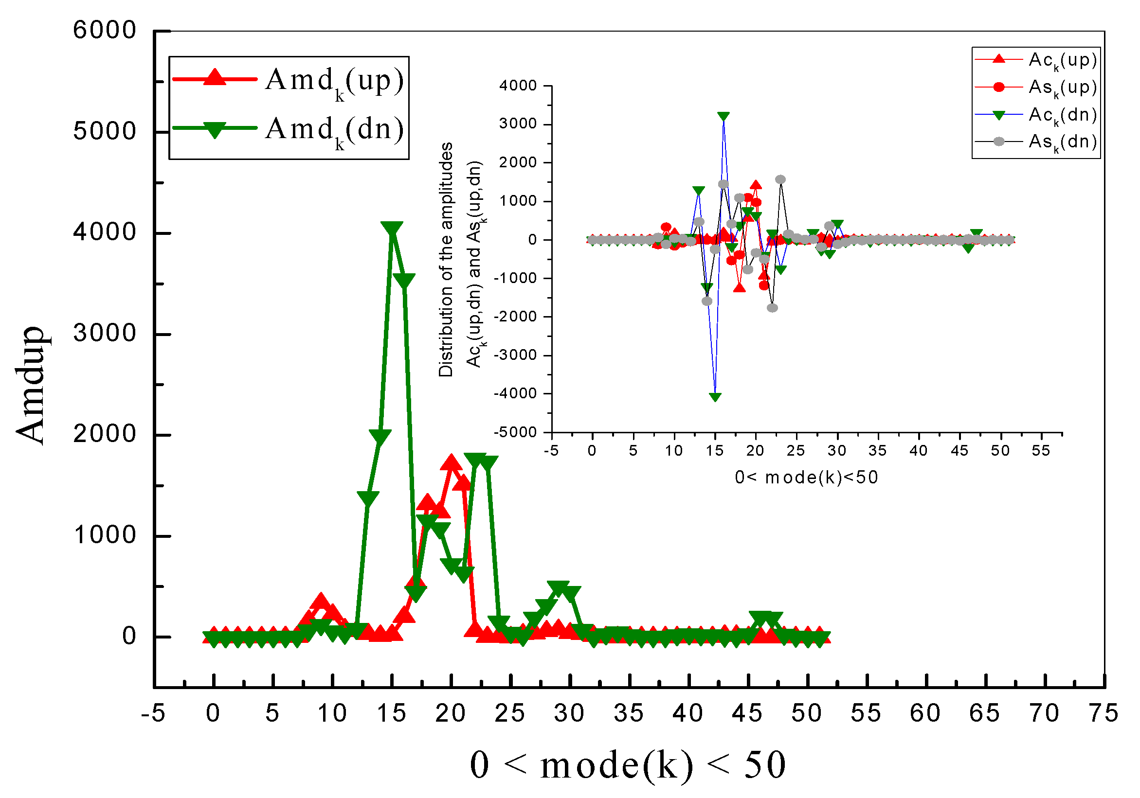
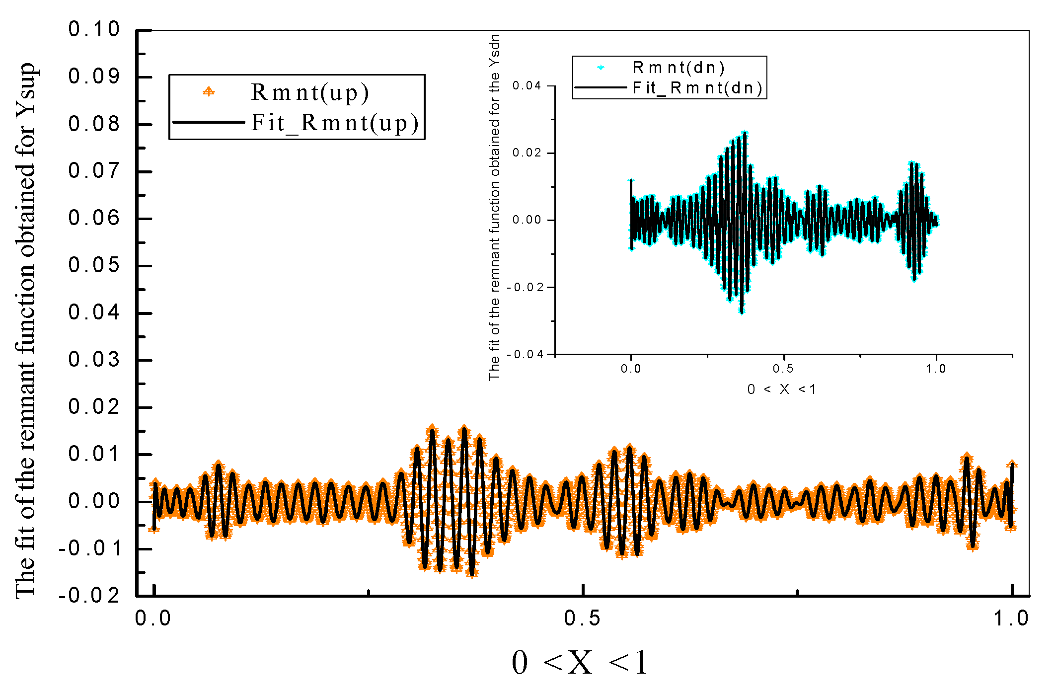
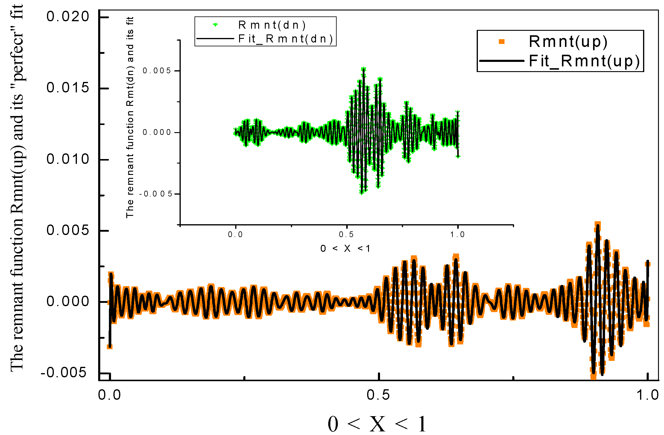
On the Internet, one can easily find many examples of different acoustic data. An acoustic signal, in the most cases, represents itself as an irreproducible AP signal. We should select rather small acoustic fragments (not exceeding one minute). Therefore, one can visit the site https://soundspunos.com/, accessed on 13 June 2023, where different sounds are collected, and these data can be downloaded by a potential user free of charge. From this site, one can select the short fragments of two insects that are the best known by each person: (1) the sound of a flying bee, and (2) the sound of a female mosquito flying up to a person. For treatment of these data, we reduced the initial data to three incident points (R-3IP). This method was described in paper [36]. It helps to receive three types of data: (a) the distribution of the upper amplitudes (Yup); (b) the distribution of the down amplitudes (Ydn); and (c) the averaged amplitudes (Ymn). In our case, the length of the compressed parameter b = 100. This procedure helps to extract the low-frequency envelopes. After that, we applied the optimal linear smoothing procedure (POLS), which was described in papers [36,37]. The POLS method helps to smooth initial data, to partly remove the high-frequency fluctuations, and to receive the desired low-frequency envelopes. These smoothed envelopes are described as Ysup and Ysdn distributions and these two smoothed curves can be considered as the prepared data files for the application of the NAFASS method. In addition, we selected 1500 data points for each chosen acoustic fragment and normalized the abscissa values to the unit value. The desired data obtained from the sounds of the buzzing bee are shown in Figure 12. The prepared smoothed envelopes for the NAFASS approach are shown by bold black lines. After preparation of the desired smoothed data, the proposed algorithm (S1–S3) of the data treatment was applied, as described above. In order to justify the selection of hypothesis (3) for this case, we were forced to show only the key figures. Figure 13 shows the distributions of the relative errors for the two branches Ysup(x) and Ysdn(x). These curves help in calculating the optimal frequency branch and realizing the desired fit for the selected envelopes. The final fit for these curves is shown in Figure 14. The AFRs for these smoothed curves are shown in Figure 15. We observed again this “quasi-resonance” behavior of the module A m d k = A c k 2 + A s k 2 and the decomposition coefficients Ack and Ask that were mentioned earlier for economic data. The plots presented in Figure 16 confirm again the justification of the GGM (3) for the fitting of the optimal frequency branch Ωk. The corresponding fitting functions in the forms (11) and (3) for both optimal frequency branches are shown in Figure 17. In order to find additional proof in favor of the selection of hypothesis (2), we extended the fitting function (11) to the limits (0 < mode(q) < 100). This extended function should fit the remnant function Rmnt(X) as the difference between the smoothed functions and their fitted replicas, as depicted in Figure 14. This “perfect” fit (with the value of the relative error < 1.0%) for both functions Rmnt(up) and Rmnt(dn) is shown in Figure 18. We were forced to omit their AFR plots (they are similar to the behavior shown in Figure 10) in order to include some figures related to the second insect.
In order not to overload this paper content with a large number of figures, we placed only the key figures that can justify the hypotheses (3) and (11). Figure 19 shows the smoothed envelopes (the desired aperiodic signals) prepared from this acoustic file related to the second insect. They are marked with solid black curves. We were forced to skip the intermediate processing steps and to show only the final fit that solved the first problem. This is shown in Figure 20. We should emphasize again that Figure 21 confirms the choice of hypotheses (3) and (11) for these smoothed envelopes depicted in the previous Figure 20. The weighting factors for two insects and other parameters, including relative fitting errors for the distribution of the frequencies, are provided in Table 4, Table 5 and Table 6. As an additional argument justifying the choice of hypotheses (3) and (11), we present the fit of the remnant functions that are similarly obtained for acoustic data (see Figure 18 and Figure 22) for insects (1) and (2), respectively. They were obtained in a similar way. We again increased the number of modes to 0 < mode(q) < 100 again and, then, used this modified frequency branch for the fitting of the remnant functions obtained as the differences between the smoothed envelopes and their fitted copies. Therefore, the selected set of aperiodic signals that were obtained independently from different sources confirmed hypotheses (3) and (11).

4. Discussion and Conclusions

In this work, we clearly demonstrated how to match a variety of stationary aperiodic signal sets with a discrete frequency structure. For the purposes of describing this class of irreproducible signals, we chose the correct formula as the general fitting Function (1). According to a detailed analysis, it was also necessary to solve the second problem, which involves using the best frequency branch Ωk, in addition to addressing the first problem by applying Formula (1) to the given signal y(t). In a prior publication [35], we used the linear-difference Equation (2), and even a portion of the Prony series, for essentially reproducible measurements. The physical significance of Equation (2), used for the fitting of the optimal frequency branch, can be repeated. In actuality, Equation (2) depicts a potential amalgamation of many beatings that may exist across linked frequencies, as was demonstrated in [35]. The more in-depth investigation carried out in this paper, however, revealed that this supposition is not accurate or ideal. Our calculations, tailored for the analysis of nonlinear difference equations, clearly demonstrate that the behavior of the estimated optimal frequency branch is described by the fitting Functions (3) and (11). In the most general example, these functions also offer the fit to the approximation function (1) for a randomly selected stationary aperiodic signal. Again, the amplitudes Ack and Ask are simple to calculate, using the LLSM. If other uncontrollable elements are deemed unimportant, the ability to identify the best frequency branch within the parameters of the defined approach opens up new opportunities for forecasting future values.
We also wish to emphasize that by introducing the power-law exponent s, which covers the well-known mean values as harmonic and geometric ones, we generalized the previously linear case to the nonlinear one (see Formulas (6) and (7)). This minor change aided in our demonstration that the generalized geometric mean corresponds to the global minimum of approximation, rather than the arithmetic mean, which is generally accepted in the field of signal processing (based on Bellman’s inequality (16)).
Another issue is the generalized NAFASS method’s use for chaotic data. How do you fix it? From our perspective, the initial step is to integrate the chaotic data relative to its mean value and reduce the high frequency oscillations. After integration, a clearly trended random curve is produced. If it is considered as an aperiodic signal, the NAFASS approach might be applied. The use of chaotic signals and the application to them of the proposed NAFASS method should be the subject of a separate investigation.
Using the resources at our disposal, we selected aperiodic signals from the Internet. Hypothesis (3) was chosen after matching analyses of economic and acoustic data were conducted. It is possible to select a suitable “candidate” for the description of a broad class of aperiodic signals, including their frequency branches, using this intriguing relationship expressed in the equivalent Form (11). Along with Hypothesis (3), we also confirmed a more straightforward combination:
Ω k + 2 = Ω k + 1 w 1 Ω k w 0   with   w 1 + w 0 = 1 .
This hypothesis also provides the desired minimal value at s = 0; however, it cannot provide the perfect minimal relative error values < 1%, as it was obtained in the case of the application of Hypothesis (3). Therefore, expression (13) can be used as an alternative hypothesis in some simple cases. The solution of the recurrence Equation (13) has the following form:
Ω k = exp ( C 0 + C 1 λ 1 k ) ,
where the constants C0,1 are found from initial conditions related with Ω0,1 and the root λ1 is related with weighting factors w0,1 by the following relationship:
λ 1 = w 0 = w 1 1 .
The reason many aperiodic signals follow the verified hypothesis (3) and are tightly associated with their optimal frequency branch can be explained as follows. If we consider [38], then one can find the proof of the following inequality that was formulated as a theorem. For any positive set of numbers x1, x2, …, xn and any set of numbers w1, w2, …, wn, satisfying the condition k = 1 n w k = 1 , the following inequality takes place:
k = 1 n x k w k   k = 1 n w k x k
The equal sign in (16) occurs if, and only if, x1 = x2 = … = xn. By identifying the set of x1, x2, …, xn with our positive set of frequencies Ω1, …, Ωn, we confirmed this Bellman inequality on real data. In fact, we obtained a new fitting function for the calculated set of frequencies associated with a wide class of stationary aperiodic signals that is expressed in the Form (6), including the limiting case (7) at s = 0.
Concluding this section, one can write an expression that connects five successive frequencies Ωk+4, …, Ωk that should form some invariant combination w2(k), w1(k), and w0(k) weakly, depending on the number of modes k, if the verified hypothesis (3) is valid. This can be derived easily from (3) and has the following form:
w 0 ( k ) = 1 Δ ( k ) ( ln [ Ω k + 4 Ω k + 3 ] · ln [ Ω k + 2 Ω k + 1 ] + ln [ Ω k + 2 Ω k + 1 ] · ln [ Ω k + 3 Ω k + 2 ] ) , w 1 ( k ) = 1 Δ ( k ) ( ln [ Ω k + 4 Ω k + 3 ] · ln [ Ω k + 2 Ω k ] ln [ Ω k + 3 Ω k + 2 ] · ln [ Ω k + 3 Ω k + 1 ] ) , Δ ( k ) = ln [ Ω k + 2 Ω k + 1 ] · ln [ Ω k + 3 Ω k + 1 ] + ln [ Ω k + 2 Ω k ] · ln [ Ω k + 2 Ω k + 1 ] , w 2 ( k ) = 1 w 1 ( k ) w 0 ( k ) .
This expression for the weight coefficients (that should have weak dependence on the value of the mode k) can serve as an additional argument in favor of the proper selection and justification of expressions (3) and (11) for the frequency branches of the fitting and is related to a wide class of aperiodic signals.
In the presence of noise, it is necessary to offer additional beneficial formulas for signal analysis. The following generally acknowledged statement (18) is usually true when noise influence is minor:
y ( t ) = S ( t ) + n ( t )
Here, y(t) are the measured data, S(t) is a signal, and n(t) is a random function associated with a noise. This expression is correct when S(t) >> n(t). The results of this investigation, however, show that when S(t) < n(t), expression (18) is not true and should be modified. Actually, in this case, a signal should be present in the provided envelopes Yup(t) and Ydn(t). This permits the following expression to be proposed for the situation S(t) < n(t):
y ( t ) = ( Y m n ( t ) + | S ( t ) | · ( Y u p ( t ) Y m n ( t ) ) Y m n ( t ) | S ( t ) | · ( Y m n ( t ) Y d n ( t ) ) ,   S ( t ) = cos ( ω ( t ) φ ( t ) ) .
Here, the Yup(t), Ydn(t) determine the “up” and “down” envelopes of a noise n(t), respectively, and Ymn(t) is its mean value. S(t) is the unit frequency/phase-modulated signal.
Any attentive reader, especially those one who is a professional in the field of signal processing, should be able to ask a valid question about the scope of the NAFASS method’s applicability. The following will be the initial response. The application of the NAFASS method does not appear to the authors to have any major limits as a novel procedure. Any such limitations can only be shown and revealed by additional research. In any event, the authors have made this new technique available to a large group of researchers for use in various areas of the signal processing discipline.

Author Contributions

Conceptualization, R.R.N. and Y.C.; methodology, R.R.N. and A.A.K.; software, R.R.N.; validation, R.R.N., A.A.K. and Y.C.; formal analysis, A.A.K.; investigation, Y.C.; resources, R.R.N.; data curation, R.R.N.; writing—original draft preparation, R.R.N. and A.A.K.; writing—review and editing, Y.C.; visualization, A.A.K.; supervision, Y.C.; project administration, Y.C.; funding acquisition, Y.C. All authors have read and agreed to the published version of the manuscript.

Funding

This research received no external funding.

Data Availability Statement

All data were obtained from reliable sources from the Internet.

Acknowledgments

The work was carried out with the financial support of the Ministry of Science and Higher Education of the RF within the framework of the “Priority 2030” program. The authors (R.R.N.) and (A.A.K.) are thankful to the support of both universities involved in the Strategic Academic Leadership Program.

Conflicts of Interest

The authors declare no conflict of interest.

Appendix A

Here, we reproduce the iteration Formula (15) from [35] that plays a key role for calculation of the possible branch of frequencies for stationary AP signals. This simple iteration formula helps to calculate the desired set of frequencies by a linear method. In order to find it, we present expression (1) in the following form:
S ( t ) = Y p ( t ) + S p ( t ) ,
where
Y p ( t ) = A 0 + A c p cos ( Ω p t ) + A s p sin ( Ω p t ) , S p ( t ) = k = 0 , k p K 1 [ A c k cos ( Ω k t ) + A s k sin ( Ω k t ) ]
The function Yp(t) satisfies to the differential equation of the second order:
( D 2 + Ω p 2 ) Y p ( t ) = C p ,   C p = A 0 / Ω p 2 ,   D d d t .
Double integration allows us to present (A3) as follows:
Y p ( t ) = Ω p 2 J 2 ( Y p ( t ) ) + C p 2 t 2 + C p 1 t + C p 0 , J 2 ( Y p ( t ) ) t 0 t ( t τ ) Y p ( τ ) d τ
The substitution of (A4) into (A1) allows us to receive the desired iteration formula as follows:
Δ [ S ( t ) ] Ω 0 2 Δ [ J 2 ( S ( t ) ) ] + C 02 Δ [ t 2 ] + C 01 Δ [ t ] , Δ [ S ( t ) ] Ω 1 2 Δ [ J 2 ( S ( t ) ) ] + C 12 Δ [ t 2 ] + C 11 Δ [ t ] + { A c 0 ( 1 Ω 1 2 Ω 0 2 ) Δ [ cos ( Ω 0 t ) ] + A s 0 ( 1 Ω 1 2 Ω 0 2 ) Δ [ sin ( Ω 0 t ) ] } , , Δ [ S ( t ) ] Ω p 2 Δ [ J 2 ( S ( t ) ) ] + C p 2 Δ [ t 2 ] + C p 1 Δ [ t ] + q p p 1 { A c q ( 1 Ω p 2 Ω q 2 ) Δ [ cos ( Ω q t ) ] + A s q ( 1 Ω p 2 Ω q 2 ) Δ [ sin ( Ω q t ) ] }
Here, double integration is determined by expression (A4) and the difference Δ[F(t)] is defined as follows:
Δ [ F ( t ) ] = F ( t ) F ( t ) ,   F ( t ) = 1 N j = 1 N F ( t j ) .
Expression (A5) can be considered as the basic recurrence/iteration formula for the given p = 0, 1, 2, …. It allows us to calculate the desired set of frequencies by a linear method, located with respect to each other in ascending order, viz.: Ω0 < Ω1 < … < ΩK−1. It is important to note here, however, that the formulas used in (A5) are approximations and are sensitive to the estimated values of the initial (inoculating) frequencies. We observe that S(t) from (1) satisfies to exact differential equation, allowing us to assess them more precisely and to account for potential deviations.
s = 0 M 1 ( D 2 + Ω s 2 ) S ( t ) = 0 ,   D d d t
Therefore, for practical calculations, one can use the set of independently calculated frequencies (Ω0, Ω1, Ω2) that follows from equations of the second, fourth, and sixth orders, correspondingly. The combination of Equation (A7) for M = 1, 2, 3, but presented in the integral form similar to (A3) and iteration Formula (A5), allows us to calculate at least three statistically close branches of inoculating frequencies that can be used to find the desired dependencies Ω k ( d ) , d = 0, 1, 2. These dependencies are used for the calculation of the mean frequency branch that is expressed by Expression (6) in the main text.

References

  1. Isermann, R.; Münchhof, M. Identification of Dynamic Systems: An Introduction with Applications; Springer: Berlin/Heidelberg, Germany, 2011; Volume 85. [Google Scholar]
  2. Mertins, A. Signal Analysis: Wavelets, Filter Banks, Time-Frequency Transforms and Applications; Wiley: Chichester, UK, 1999. [Google Scholar]
  3. Arecchi, F.; Meucci, R.; Puccioni, G.; Tredicce, J. Experimental evidence of subharmonic bifurcations, multistability, and turbulence in a Q-switched gas laser. Phys. Rev. Lett. 1982, 49, 1217–1220. [Google Scholar] [CrossRef]
  4. Chen, J.; Chau, K.; Chan, C.; Jiang, Q. Subharmonics and chaos in switched reluctance motor drives. IEEE Trans. Energy Convers. 2002, 17, 73–78. [Google Scholar] [CrossRef]
  5. Lauterborn, W.; Cramer, E. Subharmonic route to chaos observed in acoustics. Phys. Rev. Lett. 1981, 47, 1445. [Google Scholar] [CrossRef]
  6. Wilden, I.; Herzel, H.; Peters, G.; Tembrock, G. Subharmonics, biphonation, and deterministic chaos in mammal vocalization. Bioacoustics 1998, 9, 171–196. [Google Scholar] [CrossRef]
  7. Cohen, L. Time-Frequency Analysis; Prentice Hall Press: Upple Sadle River, NJ, USA, 1995; Volume 778. [Google Scholar]
  8. Almeida, L.B. The fractional Fourier transform and time-frequency representations. IEEE Trans. Signal Process. 1994, 42, 3084–3091. [Google Scholar] [CrossRef]
  9. Sejdić, E.; Djurović, I.; Stanković, L. Fractional Fourier transform as a signal processing tool: An overview of recent developments. Signal Process. 2011, 91, 1351–1369. [Google Scholar] [CrossRef] [Green Version]
  10. Su, X.; Tao, R.; Kang, X. Analysis and comparison of discrete fractional Fourier transforms. Signal Process. 2019, 160, 284–298. [Google Scholar] [CrossRef]
  11. Portnoff, M. Time-frequency representation of digital signals and systems based on short-time Fourier analysis. IEEE Trans. Acoust. Speech Signal Process. 1980, 28, 55–69. [Google Scholar] [CrossRef]
  12. Qian, S.; Chen, D. Joint time-frequency analysis. IEEE Signal Process. Mag. 1999, 16, 52–67. [Google Scholar] [CrossRef]
  13. Li, M.; Liu, Y.; Zhi, S.; Wang, T.; Chu, F. Short-time Fourier transform using odd symmetric window function. J. Dyn. Monit. Diagn. 2022, 1, 37–45. [Google Scholar] [CrossRef]
  14. Hlubina, P.; Luňáček, J.; Ciprian, D.; Chlebus, R. Windowed Fourier transform applied in the wavelength domain to process the spectral interference signals. Opt. Commun. 2008, 281, 2349–2354. [Google Scholar] [CrossRef] [Green Version]
  15. Kemao, Q. Windowed Fourier transform for fringe pattern analysis. Appl. Opt. 2004, 43, 2695–2702. [Google Scholar] [CrossRef] [PubMed]
  16. Qian, S.; Chen, D. Discrete Gabor transform. IEEE Trans. Signal Process. 1993, 41, 2429–2438. [Google Scholar] [CrossRef] [Green Version]
  17. Yao, J.; Krolak, P.; Steele, C. The generalized Gabor transform. IEEE Trans. Image Process. 1995, 4, 978–988. [Google Scholar] [PubMed]
  18. Zhao, Z.; Tao, R.; Li, G.; Wang, Y. Clustered fractional Gabor transform. Signal Process. 2020, 166, 107240. [Google Scholar] [CrossRef]
  19. Mallat, S. A Wavelet Tour of Signal Processing, 3rd ed.; Academic Press: Burlington, MA, USA, 1999. [Google Scholar]
  20. Yan, R.; Gao, R.X.; Chen, X. Wavelets for fault diagnosis of rotary machines: A review with applications. Signal Process. 2014, 96, 1–15. [Google Scholar] [CrossRef]
  21. Kumar, A. Wavelet signal processing: A review for recent applications. Int. J. Eng. Tech. 2020, 6, 12. [Google Scholar] [CrossRef]
  22. Peng, Z.K.; Peter, W.T.; Chu, F.L. A comparison study of improved Hilbert–Huang transform and wavelet transform: Application to fault diagnosis for rolling bearing. Mech. Syst. Signal Process. 2005, 19, 974–988. [Google Scholar] [CrossRef]
  23. Zayed, A.I. Hilbert transform associated with the fractional Fourier transform. IEEE Signal Process. Lett. 1998, 5, 206–208. [Google Scholar] [CrossRef]
  24. de Souza, U.B.; Escola, J.P.L.; da Cunha Brito, L. A survey on Hilbert-Huang transform: Evolution, challenges and solutions. Digit. Signal Process. 2022, 120, 103292. [Google Scholar] [CrossRef]
  25. Bhattacharyya, A.; Singh, L.; Pachori, R.B. Fourier–Bessel series expansion based empirical wavelet transform for analysis of non-stationary signals. Digit. Signal Process. 2018, 78, 185–196. [Google Scholar] [CrossRef]
  26. Chaudhary, P.K.; Gupta, V.; Pachori, R.B. Fourier-Bessel representation for signal processing: A review. Digit. Signal Process. 2023, 135, 103938. [Google Scholar] [CrossRef]
  27. Huang, N.E.; Shen, Z.; Long, S.R.; Wu, M.C.; Shih, H.H.; Zheng, Q.; Yen, N.C.; Tung, C.C.; Liu, H.H. The empirical mode decomposition and the Hilbert spectrum for nonlinear and non-stationary time series analysis. Proc. R. Soc. Lond. A Math. Phys. Eng. Sci. 1998, 454, 903–995. [Google Scholar] [CrossRef]
  28. Wu, Z.; Huang, N.E. Ensemble empirical mode decomposition: A noise-assisted data analysis method. Adv. Adapt. Data Anal. 2009, 1, 1–41. [Google Scholar] [CrossRef]
  29. Nigmatullin, R.R.; Khamzin, A.A.; Machado, J.T. Detection of quasi-periodic processes in complex systems: How do we quantitatively describe their properties? Phys. Scr. 2013, 89, 015201. [Google Scholar] [CrossRef] [Green Version]
  30. Nigmatullin, R.; Rakhmatullin, R. Detection of quasi-periodic processes in repeated measurements: New approach for the fitting and clusterization of different data. Commun. Nonlinear Sci. Numer. Simul. 2014, 19, 4080–4093. [Google Scholar] [CrossRef]
  31. Nigmatullin, R.R. Detection of Quasi-Periodic Processes in Experimental Measurements: Reduction to an “Ideal Experiment”. In Complex Motions and Chaos in Nonlinear Systems, Nonlinear Systems and Complexity; Springer: Berlin/Heidelberg, Germany, 2016; pp. 1–37. [Google Scholar]
  32. Nigmatullin, R.R.; Maione, G.; Lino, P.; Saponaro, F.; Zhang, W. The general theory of the quasi-reproducible experiments: How to describe the measured data of complex systems? Commun. Nonlinear Sci. Numer. Simul. 2017, 42, 324–341. [Google Scholar] [CrossRef]
  33. Tenreiro Machado, J.A.; Lopes, A.M. Approximation of data using non-integer harmonics series. Nonlinear Dyn. 2017, 89, 2845–2854. [Google Scholar] [CrossRef]
  34. Nigmatullin, R.R.; Alexandrov, V.S.; Agarwal, P.; Jain, S.; Ozdemir, N. Description of multi-periodic signals generated by complex systems: NOCFASS-New possibilities of the Fourier analysis. Numer. Algebra Control. Optim. 2022, 1–19. [Google Scholar] [CrossRef]
  35. Nigmatullin, R.R.; Gubaidullin, I.A. NAFASS: Fluctuation spectroscopy and the Prony spectrum for description of multi-frequency signals in complex systems. Commun. Nonlinear Sci. Numer. Simul. 2018, 56, 252–269. [Google Scholar] [CrossRef]
  36. Baleanu, M.C.; Nigmatullin, R.R.; Okur, S.; Osakoglu, K. New Approach for Consideration of Adsorption/Desorption Data. Commun. Nonlinear Sci. Numer. Simul. 2011, 16, 4649–4656. [Google Scholar] [CrossRef] [Green Version]
  37. Ciurea, M.L.; Lazanu, S.; Stavarache, I.; Lepadatu, A.M.; Iancu, V.; Mitroi, M.R.; Baleanu, C.M. Stress-induced traps in multilayered structures. J. Appl. Phys. 2011, 109, 013717. [Google Scholar] [CrossRef] [Green Version]
  38. Beckenbach, E.F.; Bellman, R. Inequalities; Springer Science & Business Media: New York, NY, USA, 2012; Volume 30. [Google Scholar]
Figure 1. The distribution of the monthly prices in kilodollars/metric tons, covering the period from July 1992 to June 2022. The random function can be fitted in the frame of the NAFASS method.
Fractalfract 07 00498 g001
Figure 2. The distribution of the frequencies obtained using paper’s iteration Formula (15) on the central figure [30] is shown. The function Ω(p) uses p (p = 0, 1, 2) calculated frequencies as inoculating frequencies. On the small left figure above we show the branches of the limiting frequencies that are used for the calculation of the optimal branch that is located between these limits.
Fractalfract 07 00498 g002
Figure 3. Behavior of the optimal error in percentages calculated with respect to expression (5). This criterion is used for selection of the optimal branch Ωk.
Fractalfract 07 00498 g003
Figure 4. The distributions of the mean frequencies Ω k = ( Ω k ( 1 ) + Ω k ( 2 ) + Ω k ( 3 ) ) / 3 (expressed in black rhombs) and optimal branch Ωk obtained with the help of expression (4) and based on the criterion of the minimal error value. As one can see from the figure, these two branches differ from each other. In this figure the asterisk sign (*) signifies the multiplication sign ×.
Fractalfract 07 00498 g004
Figure 5. The fit of the price distribution initially shown in Figure 1 is in bold. The fitting error equals 2.7%. This figure also demonstrates that the first problem related to the fit of the given random function as the price distribution for Al was solved.
Fractalfract 07 00498 g005
Figure 6. The calculated amplitude-frequency response (AFR) related to the amplitudes Ack, Ask, and its modulus Amdk are shown. One can notice that this distribution of the frequency has a specific “resonance” distribution and differs from the F-transformation, where presumably we have a monotone decreasing of frequencies providing the desired convergence of the Fourier decomposition.
Fractalfract 07 00498 g006
Figure 7. This figure proves the existence of the recurrence relationship (7) for a minimal group/cluster of frequencies with p = 2. Earlier, this criterion was absent [30] and the fit of the optimal frequency curve shown in Figure 4 was based on a linear relationship with s = 1. However, this figure clearly shows that the situation with s = 0 is the most probable, in comparison with the previous case when s = 1.
Fractalfract 07 00498 g007
Figure 8. These two plots demonstrate clearly the fit of the optimal frequency curve (expressed by the crossed red balls) and two equivalent fitting functions Ωk(fit) shown in the figure and Ω k + 3 = Ω k + 2 w 2 Ω k + 1 w 1 Ω k w 0 . These fitting functions are expressed by the black solid line and the small blue rhombs, respectively.
Fractalfract 07 00498 g008
Figure 9. As another proof in favor of the selection hypothesis (3), one can continue the fitting function found for the optimal frequency spectrum Ω q ( f i t ) = exp ( C 0 + C 1 λ 1 q + C 2 λ 2 q ) for the extended interval q ∈ [0, 100] and try to fit the remnant function that presents the difference between original prices (for Al in this case) and its fitting function expressed by (1). These functions are presented in this figure by the crossed open rhombs and the solid red line, respectively. The value of the fitting error is close to 4.5%. Therefore, we consider this fit as an additional argument in favor of the selection the function (3) as the basic hypothesis for the calculated optimal Ωk shown in Figure 4.
Fractalfract 07 00498 g009
Figure 10. The AFR for the remnant function shown on the previous figure. One can notice that for small values of q, the behavior of the corresponding components is rather smooth; then, after q > 50, this behavior becomes random. It is interesting to note that we observed some specific increasing of the amplitudes. In order to fit the remnant function with the range close to the unit value, amplitudes of the order 106 are necessary. This fact remains unexplained.
Fractalfract 07 00498 g010
Figure 11. For other randomly selected metals such as Cu, Ni, and Pb and their distributions, the fitting procedure in the frame of the NAFASS method look the same and, therefore, in order to save a place for other data we omitted the details covered by the set of similar figures used for treatment of the Al prices.
Fractalfract 07 00498 g011
Figure 12. This figure explains the preparation of the desired smoothed data curves (marked here by black solid lines) for application of the NAFASS method. Two methods, R-3IP and POLS, help to remove the high-frequency fluctuations and extract the desired smoothed trends. The abscissa values are normalized to the unit value for conveniences. All data contain 1500 data points.
Fractalfract 07 00498 g012
Figure 13. Distributions of the relative errors for two smoothed curves depicted in the previous figure. Both curves have the region of minimal values shown in the closed rectangle. The exact minimal values (in %) are shown below.
Fractalfract 07 00498 g013
Figure 14. The fit of the Yup and Ydn envelopes that was realized in the frame of the NAFASS method. The minimal values of the relative errors for both curves are shown in Figure 13. The distribution of the mean values, Ymn, is not considered.
Fractalfract 07 00498 g014
Figure 15. The distributions of the amplitude modules on the central figure and in the right figure above are shown. The expansion coefficients Ack(up,dn) and Ask(up,dn), which are included in the fitting function (1) are shown in the small figure. One can notice that the behavior of these coefficients has a “quasi-resonance” character and differs from the monotonic behavior of the Fourier coefficients that should provide the convergence of the F-series.
Fractalfract 07 00498 g015
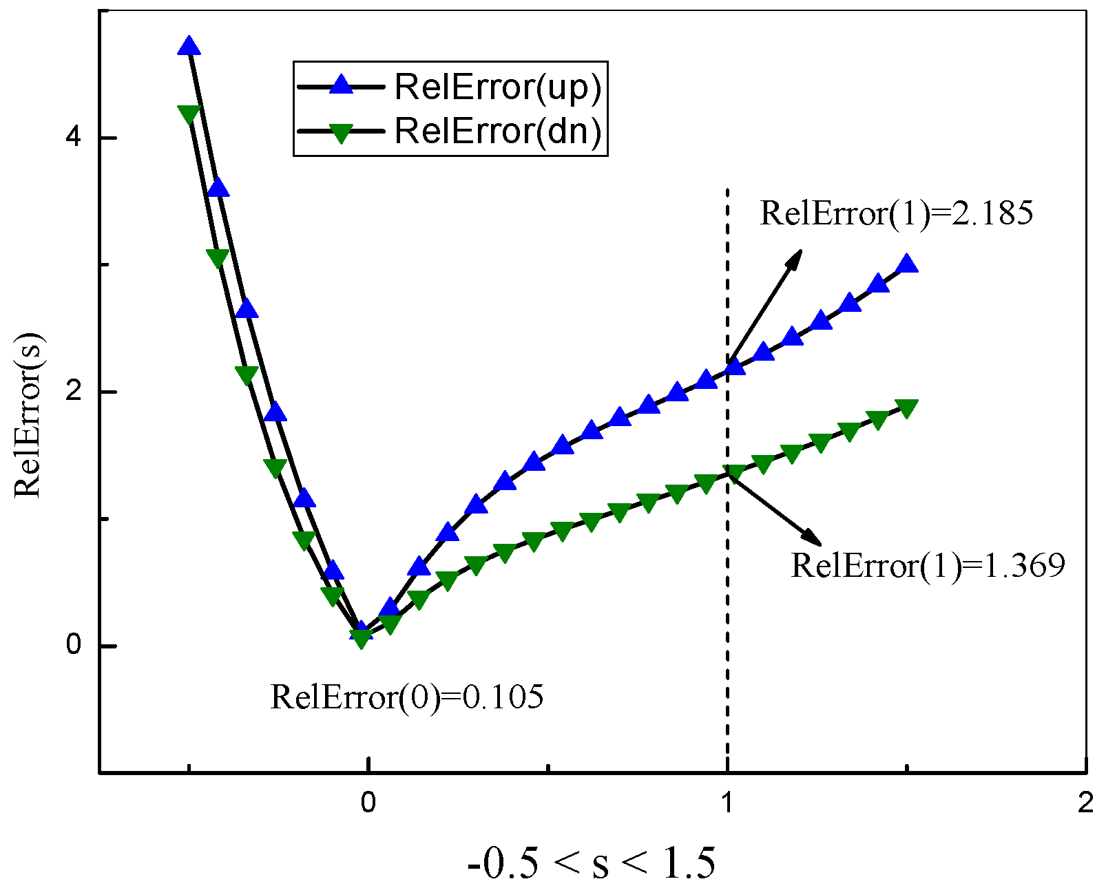
Figure 16. These plots once again prove that there is a minimum for the relative error values at s = 0. Therefore, these minimal values once again justify the choice of the fitting function (3) for the frequency distribution, which should also approximately follow expression (11).
Fractalfract 07 00498 g016
Figure 17. This figure demonstrates the fitting of the optimal branches describing the frequency distribution for the curves Yup(X) and Ydn(X), respectively. The central figure shows the corresponding branch (shown by the red crossed balls) and fitting by expression (11) and the test of expression (3). On the small figure, the similar approximation by function (11) for the down branch of frequencies is shown. The test of expression (3) is shown by red lines with small diamonds. Due to their practical fusion, they cannot be placed on the same plot.
Fractalfract 07 00498 g017
Figure 18. The fit of the remnant functions that are obtained as the differences between smoothed functions and their fit replicas depicted in Figure 14 is shown here. These curves and their “perfect” fit (the value of the relative error < 1%) can be used as additional arguments for choosing the proper hypotheses (3) and the equivalent expression (11).
Fractalfract 07 00498 g018
Figure 19. For receiving the desired smoothed curves (shown by black solid lines), one can use the same manipulation as was carried out earlier for the calculation of Figure 12. All other notations remained the same.
Fractalfract 07 00498 g019
Figure 20. We should skip the intermediate stages and, for the second insect, present the key figures only. Here, we demonstrate the final fit of two envelopes that solves the first problem.
Fractalfract 07 00498 g020
Figure 21. These two plots again confirm the choice of expressions (3) and (11). They provide the fit of the calculated optimal frequency branch. As can be seen from this figure, the earlier hypotheses selected at s = 1 were also acceptable. However, as these new results prove, the previous choice was not optimal.
Fractalfract 07 00498 g021
Figure 22. Here, a second independent argument in favor of choice of hypotheses (3) and (11) is shown. The “perfect” fit (with relative error values of 1%) is obtained for the corresponding remnant functions obtained as the difference between the functions shown in Figure 20, if it is possible to increase the number of modes to 100 using fitting function (11).
Fractalfract 07 00498 g022
Table 1. The weighting values w2,1,0 entering into expression (3) and the values of errors (in %) calculated between Ωopt and the function Ω k ( f i t ) = exp ( C 0 + C 1 λ 1 k + C 2 λ 2 k ) . The last column provides the minimal value of the error related to minimization of the RelError(s) shown in Figure 7.
Metalw2w1w0Error(Ωopt, Ωk(fit)) (%)RelError(0) (%)
Al2.53693−2.089130.55222.079770.0171
Cu2.57315−2.158590.585442.507740.00605
Ni2.58633−2.186240.599913.077690.00801
Pb2.52498−2.070130.545154.07083.3452 × 10−5
Table 2. The values of the fitting parameters that enter into the function Φ l k ( f i t ) = ln ( Ω k ) = C 0 + C 1 λ 1 k + C 2 λ 2 k .
MetalC0C1C2λ1λ2
Al0.18097−2.39532−2.62910.572650.96428
Cu0.35232−2.47294−2.610730.60420.96896
Ni0.21646−2.24152−2.55880.62230.96403
Pb−0.03681−1.79219−2.61550.572140.95284
Table 3. The basic parameters related to the fit of the price distributions.
MetalΩ0 (opt)ΩK (opt) (K = 50)A0MinErr (%)Max (Amd)
Al0.008840.79845−613.592.6058928023.2
Cu0.009980.8398814.57143.765274163.16
Ni0.011170.8771461.21086.34594759.972
Pb0.013210.8279614.14915.1413481097.5
Table 4. Weight values w2,1,0 included in expression (3) and error values (in %) calculated between Ωopt and the function Ω k ( f i t ) = exp ( C 0 + C 1 λ 1 k + C 2 λ 2 k ) . The last column provides the minimal value of the error related to minimization of the RelError(s) shown in Figure 16 and Figure 21.
Envelopes of Insectsw2w1w0Error(Ωoptk(fit)) (%)RelError(0) (%)
Ysup(1)2.62716−2.266160.639014.273660.02533
Ysdn(1)2.65023−2.308320.65814.869230.01613
Ysup(2)2.6001−2.21240.61233.442580.1051
Ysdn(2)2.67842−2.363380.684962.464990.1047
Table 5. The values of the fitting parameters included in the function Φ l k ( f i t ) = ln ( Ω k ) = C 0 + C 1 λ 1 k + C 2 λ 2 k .
Envelopes of InsectsC0C1C2λ1λ2
Ysup(1)6.04624−1.87786−2.394440.662250.96491
Ysdn(1)6.48627−2.17−2.677480.67440.97583
Ysup(2)6.18376−1.99235−2.647920.633390.96671
Ysdn(2)6.52706−2.35381−2.586880.700240.97818
Table 6. The main parameters related to the fitting of envelopes Ysup(1,2) and Ysdn(1,2) were obtained for two insects.
Envelopes of InsectsΩ0 (opt)ΩK (opt) (K = 50)A0MinErr (%)Max (Amd)
Ysup(1)6.07508306.7470.248271.3928538,985.8
Ysdn(1)5.92548348.423−0.587991.993174063.01
Ysup(2)5.30349326.0840.233010.8660789.2284
Ysdn(2)5.28291300.306−0.168510.8890314,036.72
Disclaimer/Publisher’s Note: The statements, opinions and data contained in all publications are solely those of the individual author(s) and contributor(s) and not of MDPI and/or the editor(s). MDPI and/or the editor(s) disclaim responsibility for any injury to people or property resulting from any ideas, methods, instructions or products referred to in the content.