Article

Generalized Thermoelastic Infinite Annular Cylinder under the Hyperbolic Two-Temperature Fractional-Order Strain Theory

by
Eman A. N. Al-Lehaibi
Mathematics Department, Al-Lith University College, Umm Al-Qura University, Al-Lith 21961, Saudi Arabia
Fractal Fract. 2023, 7(6), 476; https://doi.org/10.3390/fractalfract7060476
Submission received: 12 May 2023 / Revised: 8 June 2023 / Accepted: 13 June 2023 / Published: 15 June 2023
(This article belongs to the Section Mathematical Physics)

Abstract

:
This work introduces a new thermoelastic model of an isotropic and homogeneous annular cylinder. The cylinder’s bounding inner surface is shocked thermally, and the bounding outer surface has no temperature increment and volumetric strain. The governing equations in the context of the hyperbolic two-temperature generalized thermoelasticity with fractional-order strain theory have been derived. The numerical solutions of the conductive temperature, dynamic temperature, displacement, strain, and stress are illustrated in figures that use various values of fractional-order and two-temperature parameters to stand on their effects on the thermal and mechanical waves. The fractional-order parameter has significant impacts on the displacement, strain, and stress distributions. However, it does not affect dynamic or conductive temperatures. The hyperbolic two-temperature model is a successful model for making thermal and mechanical waves propagate at limited speeds.

1. Introduction

The development of engineering or mathematical models that accurately duplicates the behavior of thermoelastic materials has empirical importance in the study of materials science and solid mechanics. This field focuses on the real and physical behaviors of such substances. Hence, the engineering and mathematical models generate output and results that are consistent with laboratory observations. Scientists have created several mathematical models to describe the propagation of thermal and mechanical waves in elastic and solid materials. Despite that, not all of these models are ideal because they do not develop a model that provides finite values for the speed at which mechanical and thermal waves progress as experimental discoveries. It is necessary to explore engineering or mathematical models that study thermo-mechanical transition in thermoelastic materials. Still, we may examine models that try to produce different results that are similar to the output of the laboratory data and are compatible with our description of thermoelastic material physical behavior. Fractional calculus has numerous technical and scientific applications, including viscoelasticity, electromagnetics, electrochemistry, fluid mechanics, optics, biological population models, and signal processing. It has enabled the modeling of physical and technical processes that are most accurately characterized by fractional differential equations. The fractional derivative models are used in the process of correct modeling of those systems, namely, the damping, which requires such modeling to be exact. In these areas, in recent years, a variety of analytical and numerical approaches, as well as their applicability to new problems, have been developed [1]. Fractional differential equations, along with other complications involving special functions of mathematical physics and their extensions and generalizations in one or more variables, frequently arise when mathematical modeling is applied to real-world concerns. In addition, fractional-order PDEs are responsible for controlling most physical phenomena within their domains of validity. This includes fluid dynamics, quantum physics, electrical systems, and ecological systems, among many other models. As a result, it is becoming an increasingly necessary skill to be familiar with all of the conventional approaches, as well as the recently discovered methods for solving fractional order PDEs, as well as the implementations of these methods [1].
Many academics have been drawn to fractional calculus in the recent decade, and there have been numerous investigations published in the literature. The research focuses on the use of fractional operators in biological modeling in general [2], in physical modeling [3], in mathematical investigations and applications [4,5,6,7,8], and many other fields [9]. There are numerous fractional derivatives, but each has its own set of benefits. Most of them are aware of the difficulties: the Riemann–Liouville derivative and its associated integral are fractional operators; the Atangana–Baleanu fractional operator and its related integrals, as well as the Caputo derivative; the Caputo–Fabrizio derivative and the integral that goes with it; and the conformable derivative and the integral that goes with it. There are other additional fractional operators, and the list is extensive. The appearance of new fractional operators multiplied several debates in this discipline, including the value of fractional operators in simulating real-world issues [10].
The size dependence of Eringen’s nonlocal elasticity was investigated by Zhang et al. using a fractional order strain in a nonlocal thermoelastic study of the multilayered structures [11]. In the context of heat conduction, Sur and Kanoria presented a new mathematical model of thermoelasticity theory that generalizes the three-phase-lag thermoelastic model and the Green–Naghdi models, both of which have thermophysical properties that vary with temperature [12]. Thermodynamic and mechanical balancing laws for nonlocal solids modeled using the fractional-order continuum theory were developed by Sai et al. in their study of the constitutive modeling of a frame-invariant fractional-order approach to nonlocal thermoelasticity in the solids [13]. For micro/nano-resonators operating in harsh environments, it is crucial to building a model for estimating thermoelastic damping (TED) based on the single-phase-lag (SPL) thermoelasticity model developed by Lord and Shulma [14], dual-phase-lag (DPL) model by Tzou [15], and the nonlocal-SPL model introduced by Guyer and Krumhansl [16].
Many authors provided their own proposals. Chen and Gurtin proposed a new thermoelastic hypothesis that depends on conductive and dynamic temperature. The heat supply is proportional to the value of the difference between these two temperatures [17]. Warren and Chen observed the propagation of the thermomechanical waves under the hypothesis of the thermoelasticity theory with two temperatures [18]. Youssef has updated this hypothesis and created generalized thermoelasticity with a two-temperature model [19]. In addition, Youssef and Elsibai improved the two-temperature thermoelasticity theory to include the case of thermoelasticity without energy dissipation, as exemplified in Green–Naghdi [20,21,22]. Some applications and studies have been performed by using this theorem [23,24,25,26,27]. Youssef and El-Bary proved that the generalized thermoelasticity based on two-temperature consideration does not guarantee finite speed during the propagation of thermal waves [28]. Thus, this model was modified to work with the hyperbolic two-temperature generalized thermoelasticity theory on different heat conduction rules [28]. Youssef assumed this and reasoned that the supply of heat is proportional to the temperature differential between the conductive and thermal components as they go through the materials. In this arrangement, the rate of communication is capped. The idea of fractional calculus is used in several frameworks. Magin and Royston provided the first model to characterize the behaviors of the material by use of the concept of deformation with a fractional order [29]. The derivative of a Hookean solid is zero, while that of a Newtonian fluid is one. Both thermoelastic and thermo-viscoelastic materials have order parameters that are fractional and fall beyond the range of zero to one [29].
Youssef proposed a novel theory of generalized thermoelasticity that depends on the strain based on the definition of the fractional-order derivative. It is a variant of the Duhamel–Neumann stress–strain equation [30]. Furthermore, Youssef applied the models of Biot, Green–Lindsay, Lord–Shulman, and Green–Naghdi type-II, as well as the fractional-order strain thermoelasticity model to obtain the solutions for the one-dimensional thermoelastic half-space [30,31]. Moreover, Youssef proposed many applications for the thermoelastic nature of infinite thermoelastic cylindrical medium [25,27,32,33,34]. Using the hyperbolic two-temperature thermoelasticity, Youssef et al. investigated the produced temperature and stress fields in an elastic infinite medium containing a cylindrical hollow [25].
In this study, we provide a novel thermoelastic model of an isotropic and homogeneous annular cylinder. The exterior surface of the cylinder does not experience any kind of temperature rise or volumetric strain, but the inner surface does. Hyperbolic two-temperature generalized thermoelasticity with fractional-order strain theory has been taken into account, along with its governing equations. In this paper, we will examine how a hyperbolic two-temperature parameter, in addition to a fractional-order strain parameter, might modify the propagation of thermal and mechanical waves in thermoelastic media.

2. The Governing Equations

To derive the governing equations of the proposed problem, we presume that the region Ω = r , ψ , z :   r 1 r r 2 ,   0 ψ 2 π ,   < z < is filled with an isotropic and thermoelastic cylindrical material. We can use the cylinder’s coordinate system r , ψ , z ; t , where the z-axis is parallel to the axis of the cylinder, as seen in Figure 1. Moreover, consider the medium to be one-dimensional due to its symmetry.
Additionally, all the functions of states will depend on the time t radial and distance r . It is proposed that there are no external body forces or external heat sources in the medium and initially at rest.
After deriving the governing partial differential equations in the context of the Caputo fractional derivatives, the Laplace transformations will be applied concerning the time’s variable and convert the governing equations to ordinary differential equations. Therefore, the general solutions in the Laplace transform domain will be obtained for any set of boundary conditions. Hence, by applying certain boundary conditions, particular solutions of all the studied functions will be obtained. Finally, the inversions of the Laplace transformations will be calculated numerically by using the iteration method of Tzou; then, the numerical results will be illustrated in the figures.
As a result, the displacement components take the form of u r , u ψ , u z = u r , t , 0 , 0 , which makes the governing equations be written as [25,27,30,32,33,34,35,36]:
The equation of motion in one dimension [27,28,30,36]:
ρ 2 u r , t   t 2     = λ + 2 μ 1 + τ α D t α     e r , t   r γ   θ r , t   r     .
The heat conduction equation [27,28,30,36]:
  2 φ r , t = ρ   C E K   t + τ o   2   t 2   θ r , t +   T o γ K     t + τ o   2   t 2 1 + τ α D t α e r , t ,
and
2 φ r , t t 2 2 θ r , t t 2 = c 2 2 φ r , t ,
where θ refers to the dynamic temperature increment, while φ refers to the conductive temperature increment. c m   s 1 does not change (this is the parameter for the hyperbolic two-temperature theory). Due to the symmetry of the medium along the z-axis, the heat conduction along the circumferential direction has been neglected.
Then, the constitutive relations are in the following forms [27,28,30,36]:
σ r r r , t = 1 + τ α D t α λ e r , t + 2   μ     u r , t   r γ   θ r , t ,
σ ψ   ψ r , t = 1 + τ α D t α λ   e r , t + 2   μ   u r , t r γ   θ r , t ,
σ z z r , t = 1 + τ α D t α λ e r , t γ θ r , t ,
and
σ z   r = σ ψ   r = σ z   z = 0 .
We take e as volume dilatation. This satisfies
e = 1 r   r   u r , t r ,
where 2 = 1 r r + 2 r 2 .
The Caputo fractional derivatives become:
D t α f t = 1 Γ 1 α 0 t f υ t υ α   d υ ,           t > 0 ,       1 > α > 0 .
To keep matters simple, the following non-dimensional values are used [27,32,33]:
r , u , a = c o η   r , u , a ,       t , τ , τ o = c o 2 η   t , τ , τ o ,         θ , φ = 1 T 0 θ , φ ,         σ = σ μ ,
where c o 2 = λ + 2   μ ρ , and η = ρ   C E K .
After suppressing the primes for simplicity, Equations (1)–(6) take the following forms:
2 e r , t   t 2 = 1 + τ α D t α   2 e r , t b 2 θ r , t   ,
  2 φ r , t =   t + τ o   2   t 2   θ r , t +   ε   1 + τ α D t α   e r , t ,
2 φ r , t t 2 2 θ r , t t 2 = c ˜ 2 2 φ r , t ,
σ r r r , t =   1 + τ α D t α β 2 e r , t 2 u r , t r ε 1   θ r , t ,
σ ψ ψ r , t = 1 + τ α D t α β 2 e r , t 2   u r , t   r ε 1   θ r , t ,
σ z z r , t = β 2 2 1 + τ α D t α   e r , t ε 1     θ r , t ,
where γ = 3 λ + 2 μ   α T , ε 1 = γ T o μ , ε = γ ρ   C E , β = λ + 2 μ μ 1 2 , b = ε 1 β 2 , c ˜ 2 = c 2 c o 2 .
We will apply the well-known Laplace transform, which is given as follows:
f ¯ r , s = L f r , t = 0 f r , t   e s t d t .
We may put the Laplace transform of the fractional-derivative as follows [37]:
L D t α f r , t = s α f ¯ r , s s α 1 f r , 0 ,               0 < α < 1 .
We consider the initial conditions as follows:
u r , 0 , e r , 0 , u r , 0 , e r , 0 = 0 ,               0 < α < 1 ,
and
θ r , t t = 0 = φ r , t t = 0 = θ r , t t t = 0 = φ r , t t t = 0 = 0 .
Hence, the Equations (11)–(16) take the following forms:
1 + τ α s α   2 e ¯ r , s   = s 2 e ¯ r , s + b 2 θ ¯ r , s ,
  2 φ ¯ r , s = s + τ o s 2   θ ¯ r , s +   ε   1 + τ α s α   e ¯ r , s ,
φ ¯ r , s θ ¯ r , s = δ 2 2 φ ¯ r , s ,
σ ¯ r r r , s = 1 + τ α s α   β 2 e ¯ r , s 2 u ¯ r , s r ε 1   θ ¯ r , s ,
σ ¯ ψ ψ r , s = 1 + τ α s α β 2 e ¯ r , s 2   u ¯ r , s   r ε 1 θ ¯ r , s ,
σ ¯ z z r , s = β 2 2 1 + τ α s α   e ¯ r , s ε 1     θ ¯ r , s ,
and
e ¯ = u ¯ r , s r + u ¯ r , s   r = 1 r     r   u ¯ r , s r ,
where δ 2 = c ˜ 2 s 2 .
The Equations (21)–(23) take the following forms:
  2 e ¯ r , s   = α 1 2 θ ¯ r , s + α 2 e ¯ r , s ,
  2 φ ¯ r , s =   α 3 θ ¯ r , s +   α 4   e ¯ r , s ,
and
θ ¯ r , s = φ ¯ r , s δ 2 2 φ ¯ r , s ,
where α 1 = b 1 + τ α s α , α 2 = s 2 1 + τ α s α , α 3 = s + τ o s 2 , α 4 = ε     s + τ o s 2 1 + τ α s α .
By substituting from the Equation (30) in the Equation (28), we obtain
  2   α 2 e ¯ r , s = α 1 2 δ 2 4 φ ¯ r , s .
By substituting the Equation (30) in the Equation (29), we obtain
  2 α 5 φ ¯ r , s = α 6   e ¯ r , s ,
where α 5 = α 3 1 + α 3 δ 2 and α 6 = α 4 1 + α 3 δ 2 .
By substituting from Equation (32) into the Equation (30), we obtain
θ ¯ r , s = α 7 φ ¯ r , s   α 8 e ¯ r , s ,
where α 7 = 1 δ 2 α 5 , and α 8 = δ 2 α 6 .
If we eliminate e ¯ from (31) and (32), we obtain
  4 L 2 + M φ ¯ r , s   = 0 .
Similarly, if we eliminate φ ¯ from (31) and (32), we obtain
  4 L 2 + M e ¯ r , s   = 0 ,
where L = α 2 + α 5 + α 1 α 6 1 + δ 2 α 1 α 6 , and M = α 2 α 5 1 + δ 2 α 1 α 6 .
The solutions for (34) and (35) are
φ   r , s =   α 6 i = 1 2 A i I 0 k i r + B i K 0 k i r ,
and
e ¯   r , s = i = 1 2 k i 2 α 5 A i I 0 k i r + k i 2 α 5 B i K 0 k i r ,
where I 0 * and K 0 * are the modified forms of the Bessel functions of the first and second kinds of order zero, respectively. A i ,   B i are some constants that must be determined. The constants ± k 1   and     ± k 2 are the solutions or roots of the following:
k 4 L   k 2 + M = 0 .
By substituting from the Equations (36) and (37) in the Equation (33), we obtain the equation of the dynamical temperature increment. Hence, we obtain
θ ¯ r , s = i = 1 2 α 6 α 7   α 8 k i 2 α 5 A i I 0 k i r + α 6 α 7 α 8 k i 2 α 5 B i K 0 k i r .
We use Equations (27) and (37) to obtain the displacement function [25]:
u ¯ r , s = 1 r r   e ¯ r , s   d r = i = 1 2 k i 2 α 5 A i r r I 0 k i r   d r + k i 2 α 5 B i r r K 0 k i r d r .
The following relation of Bessel integration can be used:
1 ζ ζ   I 0 ζ   d ζ = I 1 ζ ,         1 ζ ζ   K 0 ζ   d ζ = K 1 ζ ,
where I 1 ζ and K 1 ζ are the altered forms of the first and second kind of order one of the Bessel functions, respectively.
We subject the bounding plane of the inner surface of the cylinder r = r 1 to a thermal shock and no principal axial stress:
φ r 1 , t = φ o g t .
and
σ z z r 1 , t = 0 ,
where g t gives the time function of the thermal loading, while φ o gives the thermal loading strength, and it is constant. The bounding plane of the outer surface has no increment of conductive temperature, and no volumetric strain is as follows:
φ r 2 , t = 0 ,
and
e r 2 , t = 0 .
By applying the Laplace transformation, we obtain
φ ¯ r 1 , s = φ o g ¯ s ,
σ ¯ z z r 1 , s = 0 ,
φ ¯ r 2 , s = 0 ,
and
e ¯ r 2 , s = 0 .
To obtain the final form of the boundary condition (43), we will use the Equations (16) and (30) as follows:
e ¯ r 1 , s = α 9 φ 0 ,
where α 9 = α 7 ε 1 β 2 2 1 + τ α s α   +   α 8 ε 1 .
Applying the boundary condition, we obtain
i = 1 2 A i I 0 k i r 1 + B i K 0 k i r 1 = φ 0 g ¯ s α 6 ,
i = 1 2 k i 2 α 5 A i I 0 k i r 1 + k i 2 α 5 B i K 0 k i r 1 = α 9 g ¯ s φ 0 ,
i = 1 2 A i I 0 k i r 2 + B i K 0 k i r 2 = 0 ,
i = 1 2 k i 2 α 5 A i I 0 k i r 2 + k i 2 α 5 B i K 0 k i r 2 = 0 .
By obtaining the solution of the above system, we receive the following values:
A 1 = B 1 = K 0 k 1 r 2 α 6 α 9 + α 5 k 2 2 g ¯ s φ 0 α 6 k 1 2 k 2 2 I 0 k 1 r 1 K 0 k 1 r 2 I 1 k 1 r 1 K 1 k 1 r 1 ,
and
A 2 = B 2 = I 0 k 2 r 2 α 6 α 9 + α 5 k 1 2 g ¯ s φ 0 α 6 k 1 2 k 2 2 I 0 k 2 r 1 K 0 k 2 r 2 I 0 k 2 r 2 K 0 k 2 r 1 ,
Hence, the solutions in the domain of Laplace transform have been completed.
Regarding the thermal shock function g t , we consider that it takes the form
g t = H t ,
which is the well-known Heaviside unit step function.
Hence, we have
g ¯ s = 1 s .
In the time domain, we use Riemann-sum approximation approaches to numerically estimate the temperature increments, strains, displacements, and average stresses associated with conductivity and dynamical processes. We may reverse Laplace transform in any given function using the iteration of Tzou as follows [38]:
L 1 f ¯ r , s = f ( r , t ) = e κ t t 1 2 f ¯ r , κ + R e n = 1 N 1 n f ¯ r , κ + i   n π t ,
We define “ i ” as the imaginary number unit. “Re” refers to the real aspect of any complex number. Many different numerical experiments proved that the value κ meets the relation κ   4.7 t for a faster solution convergence [38].

3. Numerical Results and Discussion

Here we obtain the numerical findings and present them graphically to demonstrate the impact of the investigated factors on the propagation of thermal and mechanical waves in thermoelastic media. So, copper was utilized as the thermoelastic material, and the following physical constants were included in the calculations [25,39]:
ρ = 8954   kg   m 3 ,   T 0 = 293   K ,   C E = 383.1   m 2   K 1   s 2 ,   K = 386   kg   m   K 1 s 3   , λ = 7.76   10 10   kg   m 1   s 2 ,   α T = 1.78   10 5   K 1 ,   μ = 3.86   10 10   kg   m 1   s 2
Hence, we obtain the following dimensionless values of the material [25,27,32,33,39,40]:
b = 0.01047 ,   ε 1 = 0.419 ,   ε = 1.6086 ,   β 2 = 4 ,   φ 0 = 1.0 ,   τ o = 0.02 ,   τ = 0.01 ,   c ˜ = 0.1 assumed
We examine the numerical results for the variables under study on a wide range of the dimensionless radial distance r r 1 = 1.0 r r 2 = 3.0 at the value of the dimensionless time t = 0.5 .
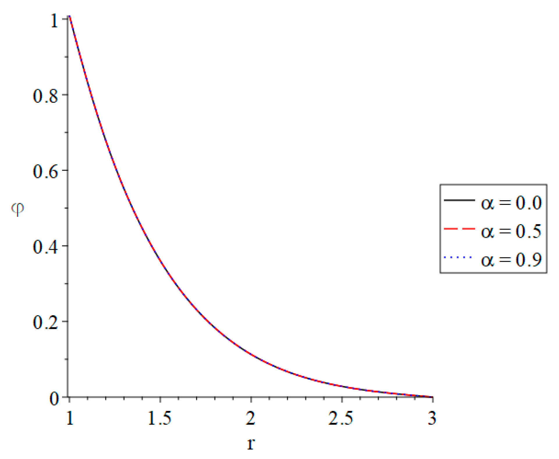
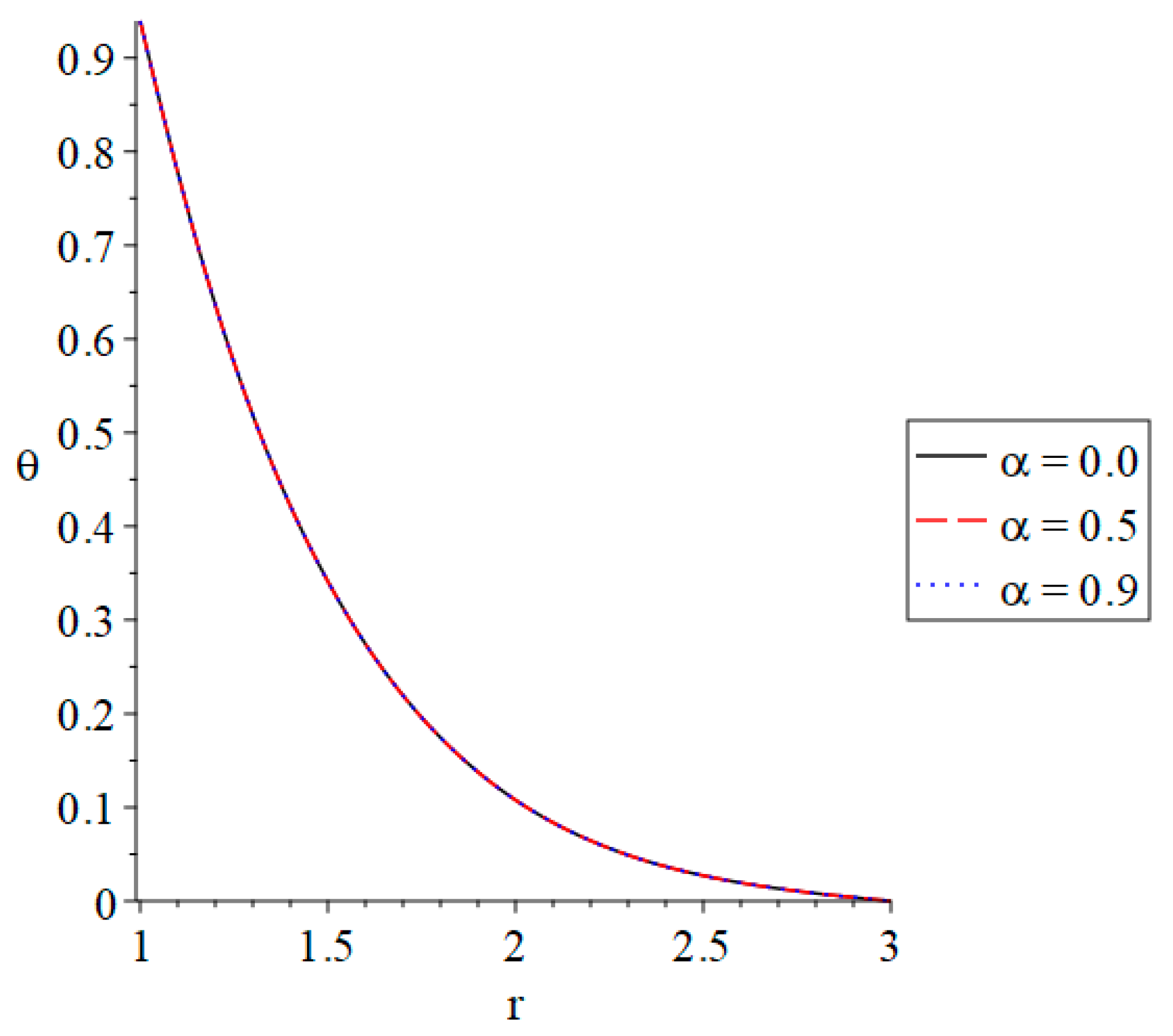
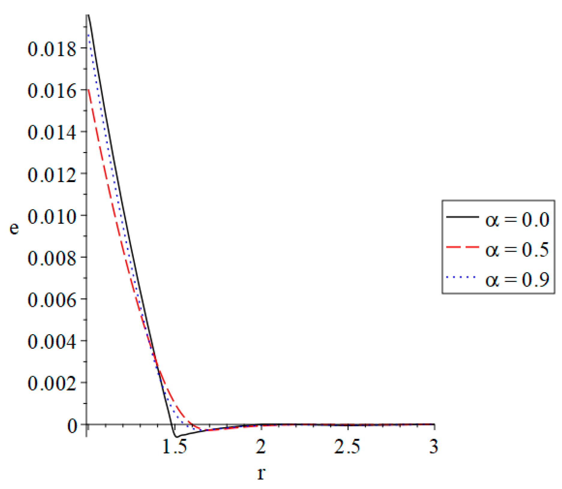
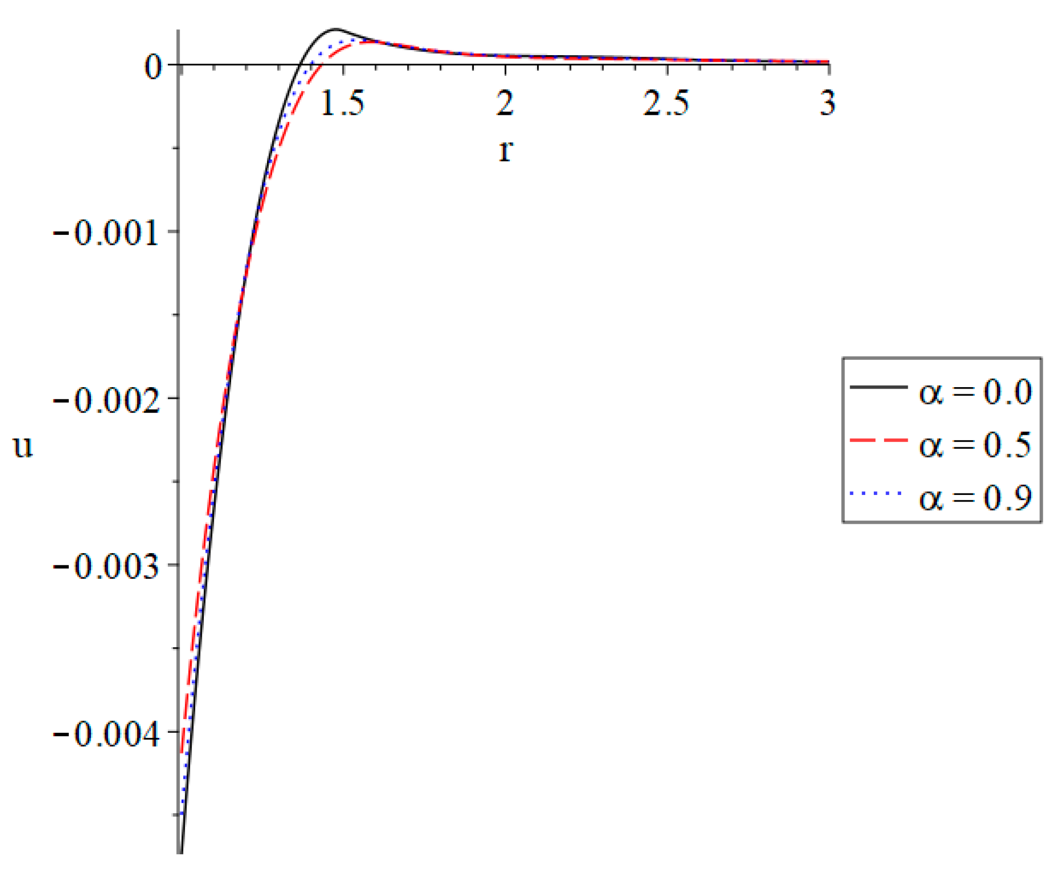
Figure 2, Figure 3, Figure 4, Figure 5 and Figure 6 show the results for values of the fractional-order strain parameter α = 0.0 , 0.5 , 0.9 in the context of the hyperbolic two-temperature thermoelasticity model to examine this parameter in the distributions understudy.
According to the results in Figure 2 and Figure 3, the impacts of the fractional-order parameter on the conductive and dynamic temperature increments are minimal. On the point r = 1.5 we have both the conductive and dynamic temperature increments in the following order:
φ , θ α = 0.0 r = 1.5 φ , θ α = 0.5 r = 1.5 < 10 5 , φ , θ α = 0.0 r = 1.5 φ , θ α = 0.9 r = 1.5 < 10 5
Furthermore, the value of the conductive temperature increment is greater than the value of the dynamical temperature increment, where we have
φ r 1 = 1.0 > θ r 1 = 0.94
On the other hand, the fractional-order strain parameter is highly impactful on distribution strains, as seen in Figure 4. In the range of distance 0 r 1.2 , the value of the strain increases when the value of the fractional order parameter increases within the range 0.0 < α < 1.0 , while the value α = 0.0 gives the larger absolute value of the strain for any value of the distance r . In the range of distance 1.2 < r 3.0 , the strain with zero fractional order parameter has a smaller value than the fractional order parameter α = 0.9 , and then α = 0.5 up to the end.
The peak value of the strain distribution rises as the fractional-order strain parameter falls in the context of strain. A strain distribution has a jump point at zero fractional order strain. The values of the strain when r = r 1 = 1.0 increase as the fractional-order strain parameter increases, and they take the following order:
e α = 0 r = r 1 > e α = 0.9 r = r 1 > e α = 0.5 r = r 1 .
The fractional-order strain parameter affects the displacement distributions, as seen in Figure 5. In the range of distance 0 r 0.75 , the absolute value of the displacement increases when the value of the fractional order parameter increases within the range 0.0 < α < 1.0 , while the value α = 0.0 gives the larger absolute value of displacement for any value of the distance r . In the range of distance 0.75 < r 3.0 , the displacement with zero fractional order parameter has a larger value than the fractional order parameter α = 0.9 , and then α = 0.5 up to the end. The highest values of the displacement distributions and their locations are different. They have the following order:
u α = 0 M a x > u α = 0.9 M a x > u α = 0.5 M a x .
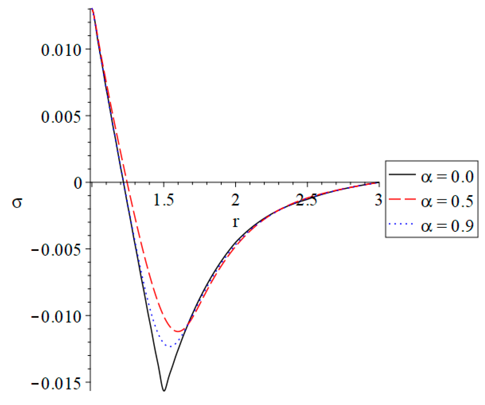
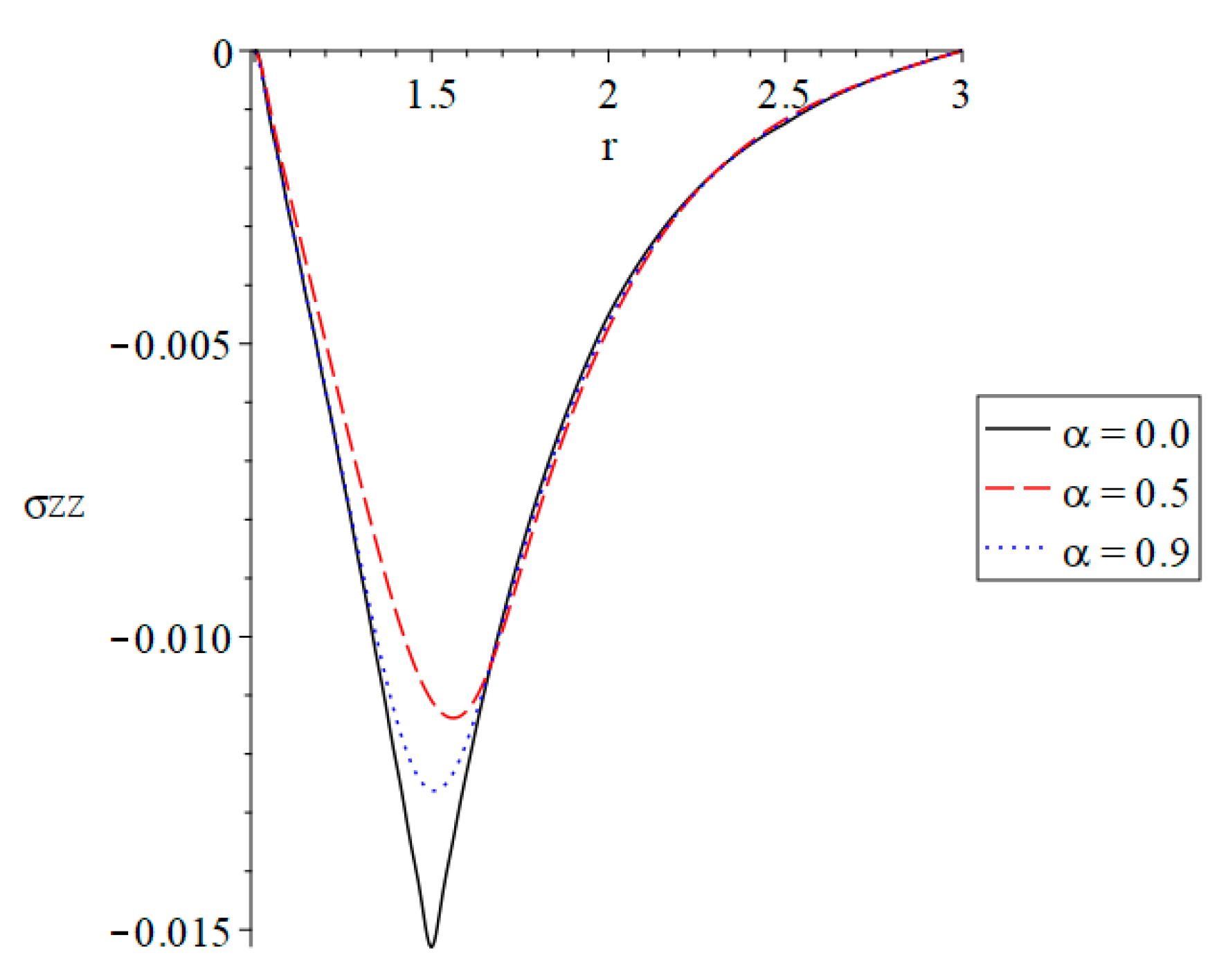
The average and axial stress distributions are affected by the fractional-order strain parameter, as illustrated in Figure 6 and Figure 7. In the range of distance 0 r 1.75 , the absolute value of the stress increases when the value of the fractional order parameter increases within the range 0.0 < α < 1.0 , while the value α = 0.0 gives the larger absolute value of stress. In the range of distance 1.75 < r 3.0 , the absolute value of stress with zero fractional order parameter has a smaller value than the fractional order parameter α = 0.9 , and then α = 0.5 up to the end. The absolute values of the peak points of the stress distributions are in various places and have distinct values, where they take the following order:
σ α = 0 M a x > σ α = 0.9 M a x > σ α = 0.5 M a x ,
and
σ z z α = 0 M a x > σ z z α = 0.9 M a x > σ z z α = 0.5 M a x .
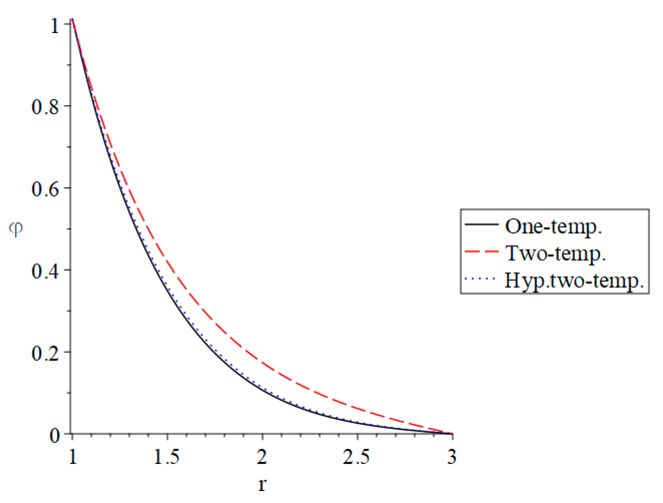
Using the fractional-order strain parameter α = 0.5 , the computations in Figure 8, Figure 9, Figure 10, Figure 11, Figure 12 and Figure 13 have been performed for several thermoelasticity models (one-temperature, two-temperature, and hyperbolic two-temperature).
Despite this, the distributions of conductive temperature increments are extremely close in both the one- and two-temperature models. Figure 8 depicts this. When compared to the other models, the classic two-temperature model’s behavior is significantly different. This means that the two-temperature model has zero intercepts before the other three models do. In other words, the classical two-temperature model has the longest-lasting effects on the propagation of thermal waves, followed by the hyperbolic two-temperature model and the one-temperature model.
The conductive temperature increment values have the following order:
φ One - temp . < φ Hyp . two - temp . < φ Two - temp . .
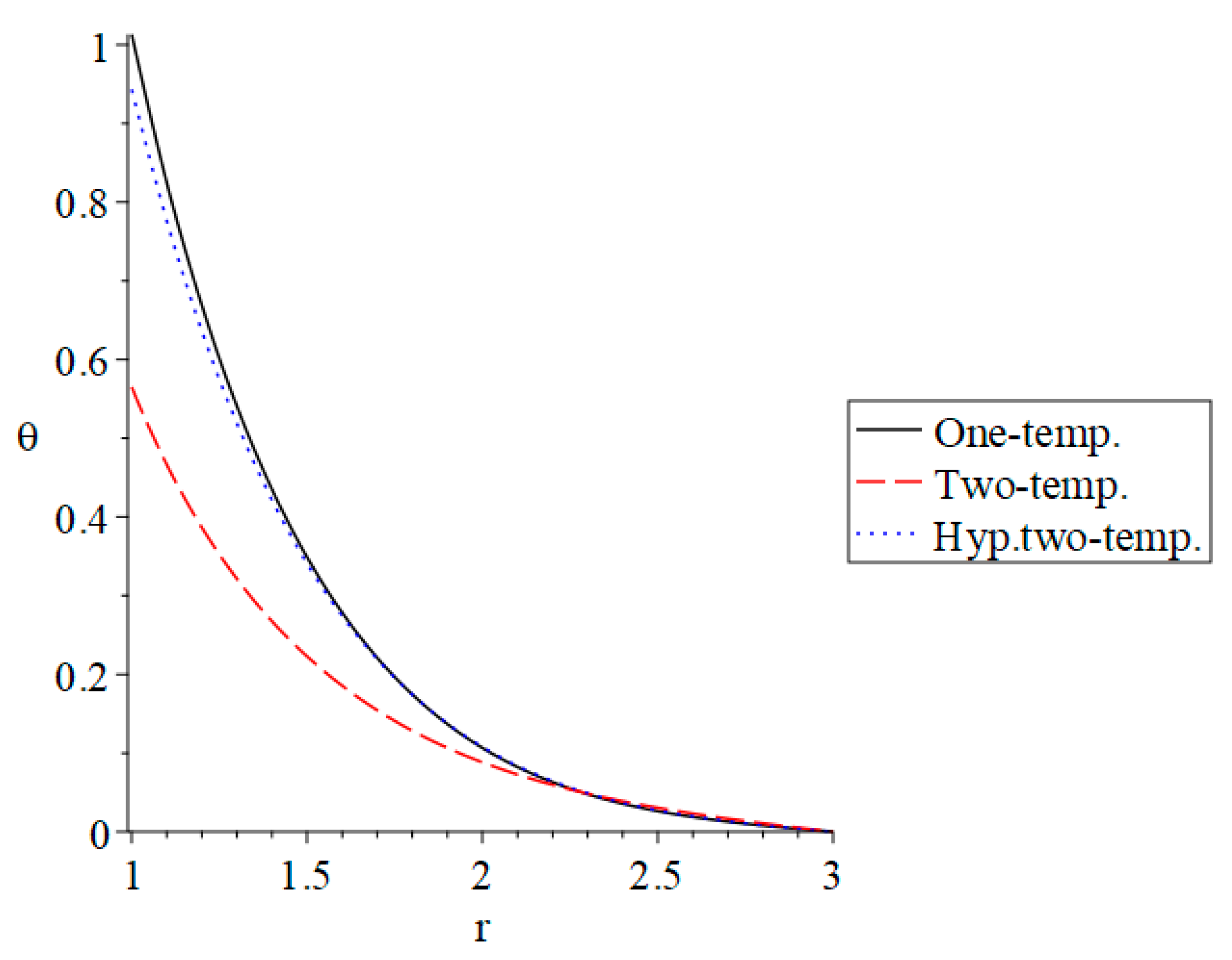
As can be seen in Figure 9, the dynamical temperature increment distributions under the hyperbolic two-temperature and one-temperature models exhibit similar behavior but have distinct values. In the setting of the standard two-temperature model, however, their behavior changes. Since the same one-temperature model is used in Figure 8 and Figure 9, the numbers for the dynamical temperature increment in Figure 9 are the same as those in Figure 8.
The dynamical temperature increment values have the following order:
θ Two - temp . < θ Hyp . two - temp . < θ One - temp . .
However, when compared to strain distributions in the traditional two-temperature model, those based on the one-temperature and hyperbolic two-temperature models exhibit equal behaviors and a wide range of values. Figure 10 clearly demonstrates this.
The strain’s starting points have the following order:
e r = r 1 Two - temp < e r = r 1 Hyp   two - temp < e r = r 1 One - temp .
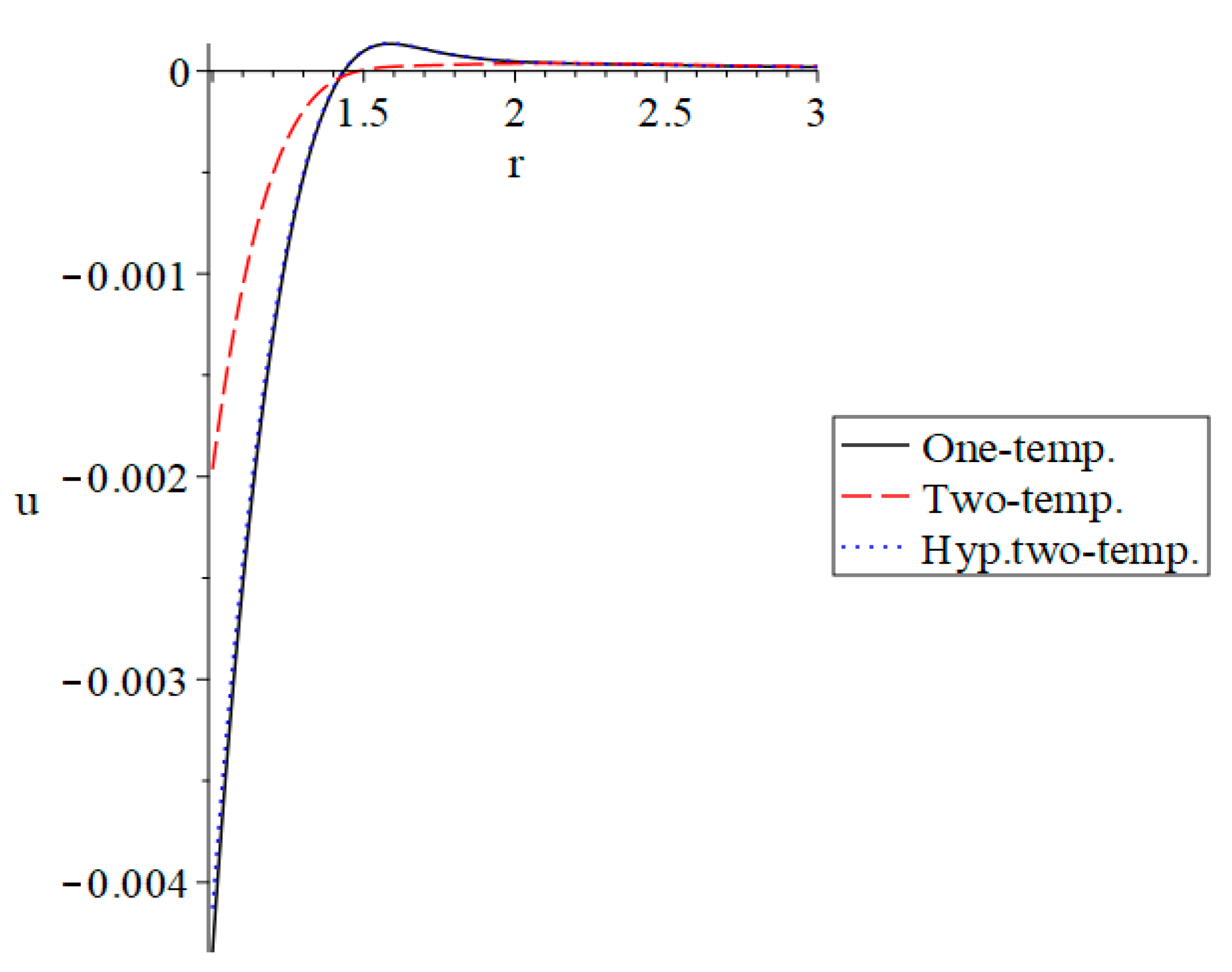
The displacement distributions in Figure 11 are shown to be closed for the one-temperature and hyperbolic two-temperature models but behave differently for the classical two-temperature model.
The displacement’s peak points are in this order:
u max Two - temp < u max Hyp   two - temp < u max One - temp .
The absolute values of the initial points of the displacement r = r 1 = 1.0 have the following order:
u r = r 1 One - temp > u r = r 1 Hyp   two - temp > u r = r 1 Two - temp .
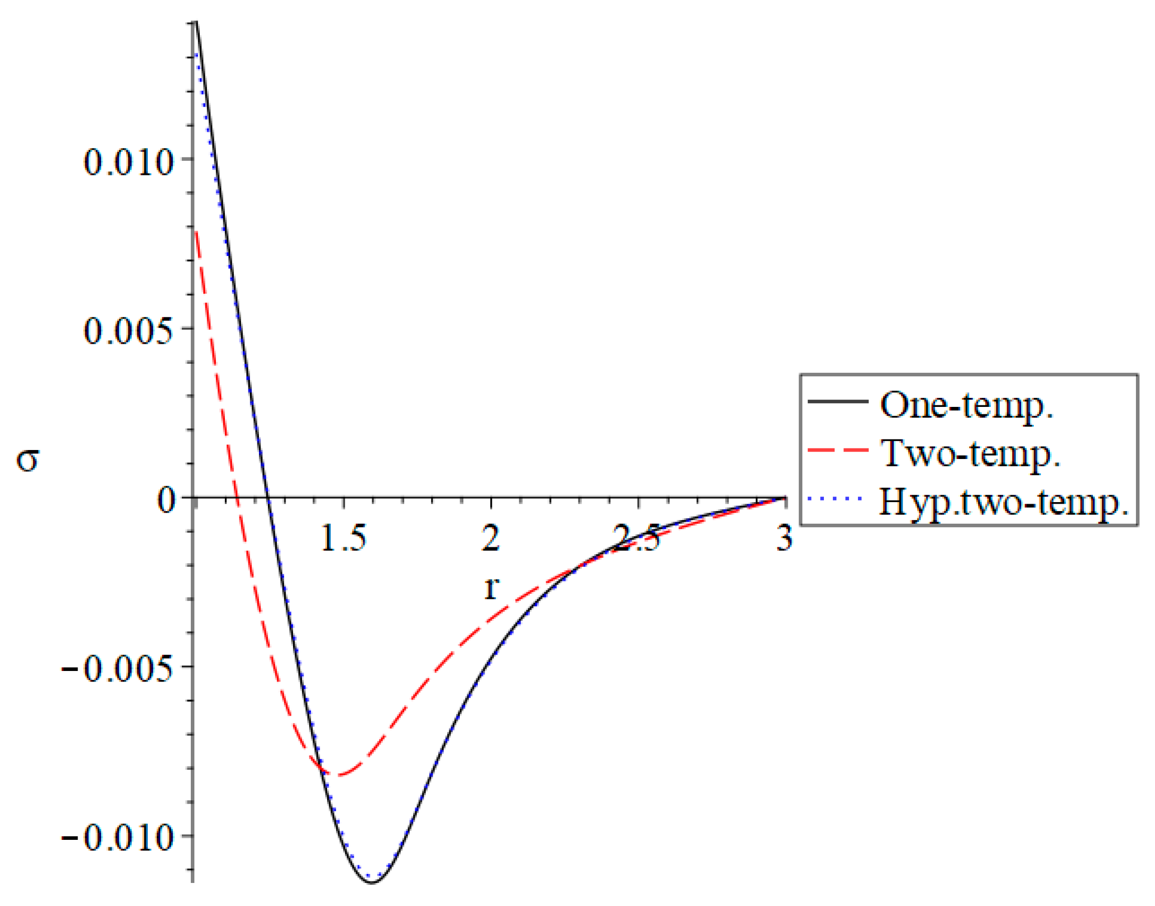
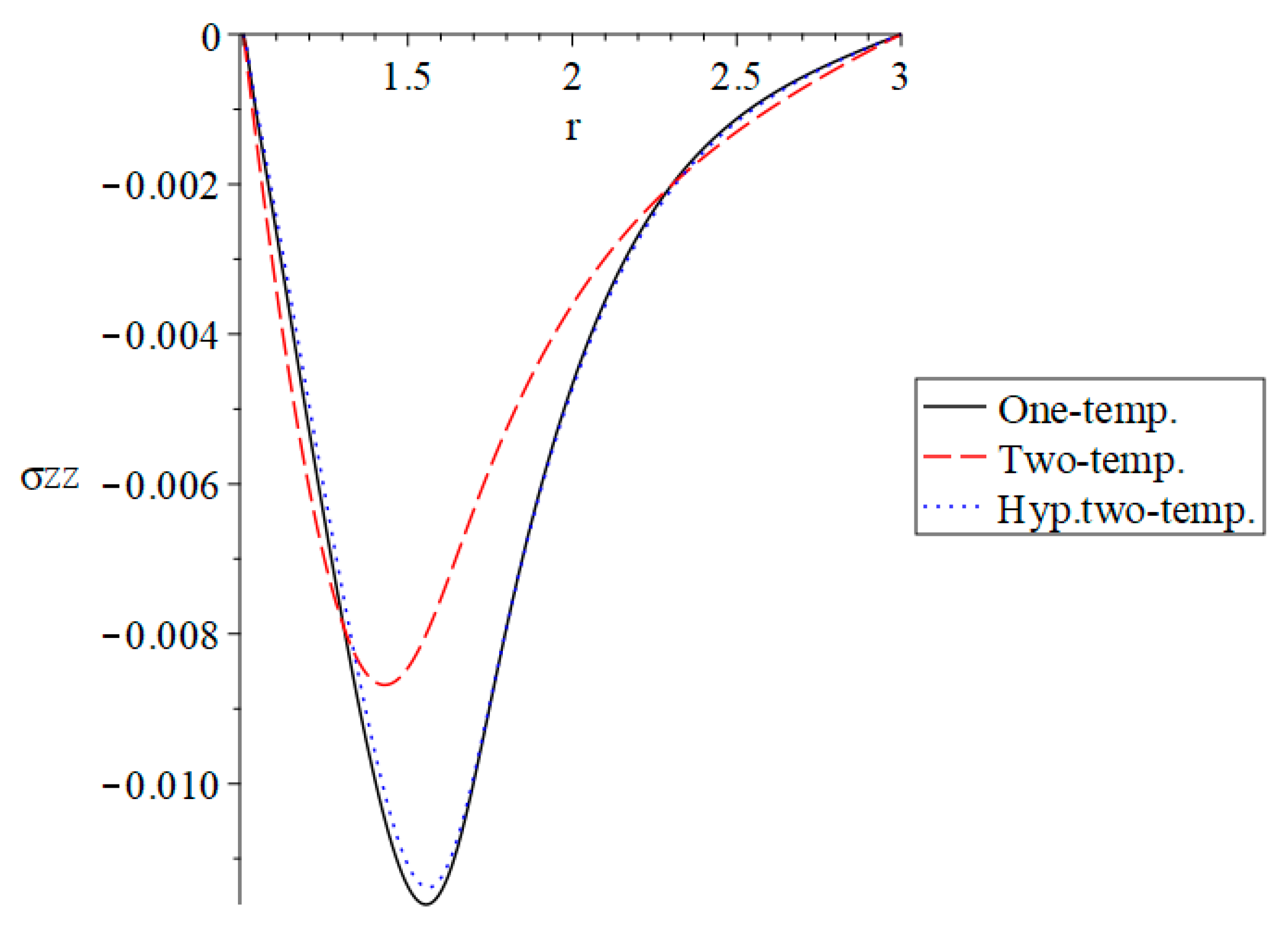
The average axial stress distributions for the one-temperature and hyperbolic two-temperature models are comparable, as shown in Figure 12 and Figure 13. However, when analyzed using the traditional two-temperature model, their behavior diverges.
Then, the absolute values of the peaks of the stress are in this order:
σ max Two - temp < σ max Hyp   two - temp < σ max One - temp ,
and
σ z z       max Two - temp < σ z z       max Hyp   two - temp < σ z z     max One - temp .
The values of the initial points of the stress r = r 1 = 1.0 take the following order:
σ r = r 1 Two - temp < σ r = r 1 Hyp   two - temp < σ r = r 1 One - temp .
In the context of considering the fractional order strain, as shown in Figure 4, Figure 6 and Figure 7, the sharp points of the strain and the stress distributions are gone. The results show that the fractional order strain theory successfully presents a model that is more in line with the actual behavior of thermoelastic materials.

4. Conclusions

It is shown numerically that the fractional-order strain parameter has negligible influence on the conductive temperature and the dynamical temperature increase. However, it has a significant effect on the strain, displacement, and stress patterns. The conventional two-temperature model of thermoelasticity, in contrast with the hyperbolic two-temperature model and the one-temperature model, produces an unlimited speed of thermal wave propagation.
As a result, the hyperbolic two-temperature thermoelasticity model helps comprehend the thermodynamic behavior of materials.
This study demonstrates that the fractional order strain theory can provide a model that is more in line with the actual behavior of thermoelastic materials.

Funding

This research received no external funding.

Data Availability Statement

All data generated or analyzed during this study are included in this published article.

Conflicts of Interest

The author has no conflict of interest to declare.

Nomenclature

C E   m 2   K 1   s 2   Specific heat at constant strain
c o     m   s 1   = λ + 2   μ ρ   Longitudinal wave speed
c m   s 1   Hyperbolic two-temperature parameter
D t α   s 1   Fractional derivative with respect to t with order α  
e   Strain or volumetric deformation (dimensionless)
K kg   m   K 1 s 3   Thermal conductivity
T     K   Absolute temperature
T 0 K   Absolute reference temperature
t   s   Time
u   m   Displacement functions
r m   The radius of the cylinder
z m   z-axis of the cylinder
α T K 1   Coefficient of linear thermal expansion
α   Fractional-order parameter (dimensionless)
β   = λ + 2 μ μ 1 2   (dimensionless)
γ kg   m 1   s 2 K 1   = 3 λ + 2 μ α T   (dimensionless)
ε   = γ ρ   C E   The mechanical coupling constant (dimensionless)
ε 1   = γ T o μ   The thermoelastic coupling constant (dimensionless)
η m 2 s     = ρ   C E K   Thermal viscosity
λ   ,   μ     kg   m 1   s 2   Lamé’s constants
ρ   kg   m 3   Density
σ i j   kg   m 1 s 2   Components of the stress tensor
τ 0 , τ s   Thermal and mechanical relaxation times, respectively

References

  1. Ray, S.S.; Atangana, A.; Noutchie, S.; Kurulay, M.; Bildik, N.; Kilicman, A. Fractional calculus and its applications in applied mathematics and other sciences. Math. Probl. Eng. 2014, 2014, 849395. [Google Scholar] [CrossRef]
  2. Sene, N. Fractional SIRI model with delay in context of the generalized Liouville–Caputo fractional derivative. Math. Model. Soft Comput. Epidemiol. 2020, 107, 107–125. [Google Scholar]
  3. Imran, M.; Shah, N.A.; Khan, I.; Aleem, M. Applications of non-integer Caputo time fractional derivatives to natural convection flow subject to arbitrary velocity and Newtonian heating. Neural Comput. Appl. 2018, 30, 1589–1599. [Google Scholar] [CrossRef]
  4. Khan, I.; Ali Shah, N.; Vieru, D. Unsteady flow of generalized Casson fluid with fractional derivative due to an infinite plate. Eur. Phys. J. Plus 2016, 131, 181. [Google Scholar] [CrossRef]
  5. Khan, I.; Ali Shah, N.; Mahsud, Y.; Vieru, D. Heat transfer analysis in a Maxwell fluid over an oscillating vertical plate using fractional Caputo-Fabrizio derivatives. Eur. Phys. J. Plus 2017, 132, 194. [Google Scholar] [CrossRef]
  6. Ali, F.; Saqib, M.; Khan, I.; Ahmad Sheikh, N. Application of Caputo-Fabrizio derivatives to MHD free convection flow of generalized Walters’-B fluid model. Eur. Phys. J. Plus 2016, 131, 377. [Google Scholar] [CrossRef]
  7. Shen, F.; Tan, W.; Zhao, Y.; Masuoka, T. The Rayleigh–Stokes problem for a heated generalized second grade fluid with fractional derivative model. Nonlinear Anal. Real World Appl. 2006, 7, 1072–1080. [Google Scholar] [CrossRef]
  8. Ganie, A.H.; Saeed, A.M.; Saeed, S.; Ali, U. The Rayleigh–Stokes Problem for a Heated Generalized Second-Grade Fluid with Fractional Derivative: An Implicit Scheme via Riemann–Liouville Integral. Math. Probl. Eng. 2022, 2022, 6948461. [Google Scholar] [CrossRef]
  9. Riaz, M.B.; Imran, M.; Shabbir, K. Analytic solutions of Oldroyd-B fluid with fractional derivatives in a circular duct that applies a constant couple. Alex. Eng. J. 2016, 55, 3267–3275. [Google Scholar] [CrossRef] [Green Version]
  10. Saad, K.M.; Baleanu, D.; Atangana, A. New fractional derivatives applied to the Korteweg–de Vries and Korteweg–de Vries–Burger’s equations. Comput. Appl. Math. 2018, 37, 5203–5216. [Google Scholar] [CrossRef]
  11. Xue, Z.-N.; Yu, Y.-J.; Li, X.-Y.; Tian, X.-G. Nonlocal thermoelastic analysis with fractional order strain in multilayered structures. J. Therm. Stress. 2018, 41, 80–97. [Google Scholar] [CrossRef]
  12. Sur, A.; Kanoria, M. Fractional order generalized thermoelastic functionally graded solid with variable material properties. J. Solid Mech. 2014, 6, 54–69. [Google Scholar]
  13. Sidhardh, S.; Patnaik, S.; Semperlotti, F. Thermodynamics of fractional-order nonlocal continua and its application to the thermoelastic response of beams. Eur. J. Mech.-A/Solids 2021, 88, 104238. [Google Scholar] [CrossRef]
  14. Lord, H.W.; Shulman, Y. A generalized dynamical theory of thermoelasticity. J. Mech. Phys. Solids 1967, 15, 299–309. [Google Scholar] [CrossRef]
  15. Tzou, D.; Guo, Z.-Y. Nonlocal behavior in thermal lagging. Int. J. Therm. Sci. 2010, 49, 1133–1137. [Google Scholar] [CrossRef]
  16. Zhou, H.; Li, P.; Fang, Y. Single-phase-lag thermoelastic damping models for rectangular cross-sectional micro-and nano-ring resonators. Int. J. Mech. Sci. 2019, 163, 105132. [Google Scholar] [CrossRef]
  17. Chen, P.J.; Gurtin, M.E. On a theory of heat conduction involving two temperatures. Z. Für Angew. Math. Und Phys. ZAMP 1968, 19, 614–627. [Google Scholar] [CrossRef]
  18. Warren, W.; Chen, P. Wave propagation in the two temperature theory of thermoelasticity. Acta Mech. 1973, 16, 21–33. [Google Scholar] [CrossRef]
  19. Youssef, H.M. Theory of two-temperature-generalized thermoelasticity. IMA J. Appl. Math. 2006, 71, 383–390. [Google Scholar] [CrossRef]
  20. Youssef, H.M.; Elsibai, K.A. On the theory of two-temperature thermoelasticity without energy dissipation of Green–Naghdi model. Appl. Anal. 2015, 94, 1997–2010. [Google Scholar] [CrossRef]
  21. Alzahrani, F.S.; Abbas, I.A. Fractional order GL model on thermoelastic interaction in porous media due to pulse heat flux. Geomech. Eng. 2020, 23, 217–225. [Google Scholar]
  22. Abbas, I.A. Fractional order GN model on thermoelastic interaction in an infinite fibre-reinforced anisotropic plate containing a circular hole. J. Comput. Theor. Nanosci. 2014, 11, 380–384. [Google Scholar] [CrossRef]
  23. Abbas, I.A.; Youssef, H.M. Two-temperature generalized thermoelasticity under ramp-type heating by finite element method. Meccanica 2013, 48, 331–339. [Google Scholar] [CrossRef]
  24. Youssef, H.M. A two-temperature generalized thermoelastic medium subjected to a moving heat source and ramp-type heating: A state-space approach. J. Mech. Mater. Struct. 2010, 4, 1637–1649. [Google Scholar] [CrossRef]
  25. El-Bary, A.A.; Youssef, H.M.; Nasr MA, E. Hyperbolic Two-Temperature Generalized Thermoelastic Infinite Medium with Cylindrical Cavity Subjected to Non-Gaussian Laser Beam. J. Umm Al-Qura Univ. Eng. Archit. 2022, 13, 62–69. [Google Scholar] [CrossRef]
  26. Youssef, H.M. Two-dimensional problem of a two-temperature generalized thermoelastic half-space subjected to ramp-type heating. Comput. Math. Model. 2008, 19, 201–216. [Google Scholar] [CrossRef]
  27. Youssef, H.M. Two-temperature generalized thermoelastic infinite medium with cylindrical cavity subjected to moving heat source. Arch. Appl. Mech. 2010, 80, 1213–1224. [Google Scholar] [CrossRef]
  28. Youssef, H.M.; El-Bary, A.A. Theory of Hyperbolic Two-Temperature Generalized Thermoelasticity. Mater. Phys. Mech. 2018, 40, 158–171. [Google Scholar]
  29. Magin, R.L.; Royston, T.J. Fractional-order elastic models of cartilage: A multi-scale approach. Commun. Nonlinear Sci. Numer. Simul. 2010, 15, 657–664. [Google Scholar] [CrossRef]
  30. Youssef, H.M. Theory of generalized thermoelasticity with fractional order strain. J. Vib. Control 2016, 22, 3840–3857. [Google Scholar] [CrossRef]
  31. Ezzat, M.A.; El-Karamany, A.S.; El-Bary, A.A. Two-temperature theory in Green–Naghdi thermoelasticity with fractional phase-lag heat transfer. Microsyst. Technol. 2018, 24, 951–961. [Google Scholar] [CrossRef]
  32. Youssef, H.M. Generalized thermoelasticity of an infinite body with a cylindrical cavity and variable material properties. J. Therm. Stress. 2005, 28, 521–532. [Google Scholar] [CrossRef]
  33. Youssef, H.M. Problem of generalized thermoelastic infinite medium with cylindrical cavity subjected to a ramp-type heating and loading. Arch. Appl. Mech. 2006, 75, 553–565. [Google Scholar] [CrossRef]
  34. Ezzat, M.; El-Bary, A. Effects of variable thermal conductivity and fractional order of heat transfer on a perfect conducting infinitely long hollow cylinder. Int. J. Therm. Sci. 2016, 108, 62–69. [Google Scholar] [CrossRef]
  35. Youssef, H.M. Two-Temperature Generalized Thermoelastic Infinite Medium with Cylindrical Cavity Subjected to Different Types of Thermal Loading. WSEAS Trans. Heat Mass Transf. 2006, 1, 769. [Google Scholar]
  36. Ezzat, M.A.; Youssef, H.M. Generalized Magneto-Thermoelasticity for an Infinite Perfect Conducting Body with A Cylindrical Cavity. Mater. Phys. Mech. 2013, 18, 156–170. [Google Scholar]
  37. Povstenko, Y. Fractional Thermoelasticity; Springer: Berlin/Heidelberg, Germany, 2015; Volume 219. [Google Scholar]
  38. Tzou, D.Y. A unified field approach for heat conduction from macro-to micro-scales. J. Heat Transf. 1995, 117, 8–16. [Google Scholar] [CrossRef]
  39. Youssef, H.M. Thermal shock problem of a generalized thermoelastic solid sphere affected by mechanical damage and thermal diffusion. J. Heat Transf. 1995, 117, 8–16. [Google Scholar] [CrossRef]
  40. Youssef, H.M. State-space approach on generalized thermoelasticity for an infinite material with a spherical cavity and variable thermal conductivity subjected to ramp-type heating. Can. Appl. Math. Quaterly 2005, 13, 4. [Google Scholar]
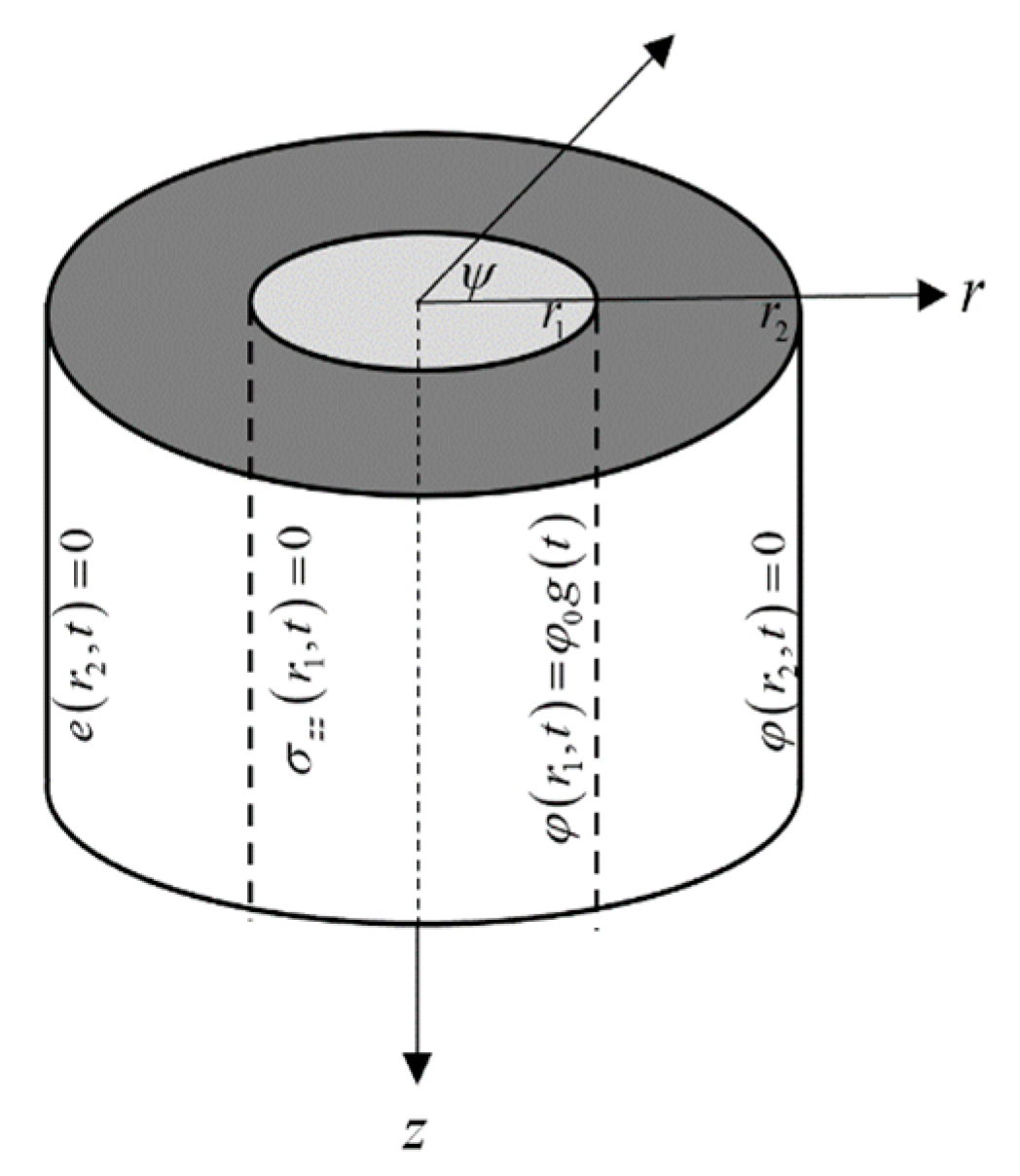
Figure 1. The annular cylindrical thermoelastic medium.
Fractalfract 07 00476 g001
Figure 2. Distribution of conductive temperature with variable values of the fractional-order strain parameter.
Fractalfract 07 00476 g002
Figure 3. Distribution of dynamical temperature with the variable values of the fractional-order strain parameter.
Fractalfract 07 00476 g003
Figure 4. Distribution of strain with the variable values of the fractional-order strain parameter.
Fractalfract 07 00476 g004
Figure 5. Distribution of displacement with the variable values of the fractional-order strain parameter.
Fractalfract 07 00476 g005
Figure 6. Distribution of average stress with the variable values of the fractional-order strain parameter.
Fractalfract 07 00476 g006
Figure 7. Distribution of axial stresses with the variable value of the fractional-order strain parameter.
Fractalfract 07 00476 g007
Figure 8. Conductive temperature increment distribution for the three models when α = 0.5 .
Fractalfract 07 00476 g008
Figure 9. Distribution of the dynamical temperature increment for the three models when α = 0.5 .
Fractalfract 07 00476 g009
Figure 10. Distribution of the strain increment for the three models when α = 0.5 .
Fractalfract 07 00476 g010
Figure 11. Distribution of displacement for the three models, when α = 0.5 .
Fractalfract 07 00476 g011
Figure 12. Distribution of average stresses for the three models, when α = 0.5 .
Fractalfract 07 00476 g012
Figure 13. Distribution of the axial stresses for the three models, when α = 0.5 .
Fractalfract 07 00476 g013
Disclaimer/Publisher’s Note: The statements, opinions and data contained in all publications are solely those of the individual author(s) and contributor(s) and not of MDPI and/or the editor(s). MDPI and/or the editor(s) disclaim responsibility for any injury to people or property resulting from any ideas, methods, instructions or products referred to in the content.