Factorized Doubling Algorithm for Large-Scale High-Ranked Riccati Equations in Fractional System

Abstract

In real-life control problems, such as power systems, there are large-scale high-ranked discrete-time algebraic Riccati equations (DAREs) from fractional systems that require stabilizing solutions. However, these solutions are no longer numerically low-rank, which creates difficulties in computation and storage. Fortunately, the potential structures of the state matrix in these systems (e.g., being banded-plus-low-rank) could be beneficial for large-scale computation. In this paper, a factorized structure-preserving doubling algorithm (FSDA) is developed under the assumptions that the non-linear and constant terms are positive semidefinite and banded-plus-low-rank. The detailed iteration scheme and a deflation process for FSDA are analyzed. Additionally, a technique of partial truncation and compression is introduced to reduce the dimensions of the low-rank factors. The computation of residual and the termination condition of the structured version are also redesigned. Illustrative numerical examples show that the proposed FSDA outperforms SDA with hierarchical matrices toolbox (SDA_HODLR) on CPU time for large-scale problems.

1. Introduction

Consider the fractional system [1,2]

$${\Delta }^{\left(\alpha \right)}x(t+1)=\mathbb{A}x\left(t\right)+\mathbb{B}u\left(t\right),y\left(t\right)=Cx\left(t\right),$$

(1)

where $\alpha \in (0,1)$ and ($\alpha$) represents the order of the fractional derivative, $\mathbb{A}\in {\mathbb{R}}^{N\times N}$, $\mathbb{B}\in {\mathbb{R}}^{N\times m}$ and $C\in {\mathbb{R}}^{l\times N}$ with $m,l\le N$. If ${\Delta }^{\left(\alpha \right)}x(t+1)$ is approximated by the Grünwald–Letnikov rule [3] at $k=1$, the system (1) is equivalent to the discrete-time linear system

$$x(t+1)=Ax\left(t\right)+Bu\left(t\right),y\left(t\right)=Cx\left(t\right),$$

(2)

where $A=h^{\alpha }\mathbb{A}+\alpha I$ and $B=h^{\alpha }\mathbb{B}$. The corresponding optimal control and the feedback gain can be expressed in terms of the unique positive semidefinite stabilizing solution of the discrete-time algebraic Riccati Equation (DARE)

$$\begin{array}{ccc}\hfill \mathcal{D}\left(X\right)& \equiv & -X+A^{\top }X{(I+GX)}^{-1}A+H=0,A,G,H\in {\mathbb{R}}^{N\times N}.\hfill \end{array}$$

(3)

There have been numerous methods, including classical and state-of-the-art techniques, developed over the past few decades to solve this equation in a numerically stable manner. See [4,5,6,7,8,9,10,11,12,13,14,15] and the references therein for more details.

In many large-scale control problems, the matrix $G=B{R}^{-1}{B}^{\top }$ in the non-linear term and $H=C^{\top }{T}^{-1}C$ in the constant term are of low-rank with $B\in {\mathbb{R}}^{N\times m^g}$, $R\in {\mathbb{R}}^{m^g\times m^g}$, $C\in {\mathbb{R}}^{m^h\times N}$, $T\in {\mathbb{R}}^{m^h\times m^h}$, and $m^g,m^h\ll N$. Then the unique positive definite stabilizing solution in the DARE (3) or its dual equation can be approximated numerically by a low-rank matrix [16,17]. However, when the constant term H in the DARE equation has a high-rank structure, the stabilizing solution is no longer numerically low-ranked, making its storage and outputting difficult. To solve this issue, an adapted version of the doubling algorithm, named SDA_h, was proposed in [18]. The main idea behind SDA_h is to take advantage of the numerical low-rank of the stabilizing solution in the dual equation to estimate the residual of the original DARE. In this way, SDA_h can efficiently evaluate the residual and output the feedback gain. An interesting question up to now is:

• Can SDA solve the large-scale DAREs efficiently when both G and H are of high-rank?

The main difficulty, in this case, lies in that the stabilizing solutions both in DARE (3) and its dual equation are not of low-rank, making the direct application of SDA difficult for large-scale problems, especially the estimation of residuals and the realization of algorithmic termination. This paper attempts to overcome this obstacle. Rather than answering the above question completely, DARE (3) with the banded-plus-low-rank structure

$$A=D^A+L_{10}^A{K}^A{\left(L_{20}^A\right)}^{\top }$$

(4)

is considered, where $D^A\in {\mathbb{R}}^{N\times N}$ is a banded matrix, $L_{10}^A$, $L_{20}^A\in {\mathbb{R}}^{N\times m^a}$ are low-rank matrices and $K^A\in {\mathbb{R}}^{m^a\times m^a}$ is the kernel matrix with $m^a\ll N$. The assumption of (4) is not necessary when G and H are of low rank, i.e., in that case A is allowed to be any (sparse) matrix. We also assume that the high-rank non-linear item and the constant item are of the form

$$G=D^G+L^G{K}^G{\left(L^G\right)}^{\top },H=D^H+L^H{K}^H{\left(L^H\right)}^{\top },$$

(5)

where $D^G$, $D^H\in {\mathbb{R}}^{N\times N}$ are positive semidefinite banded matrices, $L^G\in {\mathbb{R}}^{N\times m^g}$, $L^H\in {\mathbb{R}}^{N\times m^h}$, $K^G\in {\mathbb{R}}^{m^g\times m^g}$ and $K^H\in {\mathbb{R}}^{m^h\times m^h}$ are symmetric and $m^g,m^h\ll N$ (here $m^g$ and $m^h$ might be zero). In addition, we assume that $D^A$, $D^G$, and $D^H$ are all banded matrices with banded inverse (BMBI), which has some applications in the power system [19,20,21]. See also [22,23,24,25,26,27,28,29], as well as their references for other applications.

The main contributions in this paper are:

• Although the hierarchical (e.g., HODLR) structure [30,31] can be employed to run the SDA to cope with large-scale DAREs with both high-rank H and G, it is the first to develop SDA to the factorized form—FSDA—to deal with such DAREs.
• The structure of the FSDA iterative sequence is explicitly revealed to consist of two parts—the banded part and the low-rank part. The banded part can iterate independently while the low-rank part relies heavily on the product of the banded part and the low-rank part.
• A deflation process of the low-rank factors is proposed to reduce the column number of the low-rank part. The conventional truncation and compression in [17,18] for the whole low-rank factor does not to work as it destroys the implicit structure and makes the subsequent deflation infeasible. Instead, a partial truncation and compression (PTC) technique is then devised to impose merely on the exponentially increasing part (after deflation), effectively slimming the dimensions of the low-rank factors.
• The termination criterion of FSDA consists of two parts. The residual of the banded part is considered in the pre-termination, and only if it is small enough, the actual termination criterion involving the low-rank factors is computed. This way, the time-consuming detection of the terminating condition is reduced in complexity.

The research in this field is also motivated by other applications, such as the finite element methods (FEM). In FEM, the matrices resulting from discretizing the matrix equations exhibit a sparse and structured pattern [32,33]. By capitalizing on these advantages, iterative methods designed for such matrices can significantly enhance computational efficiency, minimize memory usage, and lead to quicker solutions for large-scale problems.

The whole paper is organized as follows. Section 2 describes the FSDA for DAREs (3) with high-rank non-linear and constant terms. The deflation process for the low-rank factors and kernels is given in Section 3. Section 4 dwells on the technique of PTC to slim the dimensions of low-rank factors and kernels. The way to compute the residual, as well as the concrete implementation of the FSDA, is described in Section 5. Numerical experiments are listed in Section 6 to show the effectiveness of the FSDA.

Notation 1.

$I_{{}_N}$ (or simply I) is the $N\times N$ identity matrix. For a matrix $A\in {\mathbb{R}}^{N\times N}$, $\rho \left(A\right)$ denotes the spectral radius of A. For symmetric matrices A and $B\in {\mathbb{R}}^{N\times N}$, we say $A>B$ ($A\ge B$) if $A-B$ is a positive definite (semi-definite) matrix. Unless stated otherwise, the norm $\parallel ·\parallel$ is the F-norm of a matrix. For a sequence of matrices ${\left\{A_i\right\}}_{i=1}^k$, ${\prod }_{i=k}^0{A}_i=A_k{A}_{k-1}\dots A_1{A}_0$. For a banded matrix B, $bw\left(B\right)$ represents the bandwidth. Additionally, the Sherman–Morrison–Woodbury (SMW) formula (see [34] for example), ${(M+UD{V}^{\top })}^{-1}=M^{-1}-M^{-1}U{(D^{-1}+V^{\top }{M}^{-1}U)}^{-1}{V}^{\top }{M}^{-1}$ is required in the analysis of iterative scheme.

2. SDA and the Structured Iteration for DARE

For DARE

$$\mathcal{D}\left(X\right)=-X+A^{\top }X{(I+GX)}^{-1}A+H=0$$

and its dual equation

$${\mathcal{D}}_a\left(Y\right)=-Y+AY{(I+HY)}^{-1}{A}^{\top }+G=0,$$

(6)

SDA [7] generates a sequence of matrices, for $k\ge 1$

$$\left\{\begin{array}{ccc}\hfill G_k& =& G_{k-1}+A_{k-1}{(I+G_{k-1}{H}_{k-1})}^{-1}{G}_{k-1}{A}_{k-1}^{\top },\hfill \\ \hfill H_k& =& H_{k-1}+A_{k-1}^{\top }{H}_{k-1}{(I+G_{k-1}{H}_{k-1})}^{-1}{A}_{k-1},\hfill \\ \hfill A_k& =& A_{k-1}{(I+G_{k-1}{H}_{k-1})}^{-1}{A}_{k-1},\hfill \end{array}\right.$$

(7)

with $A_0=A$, $G_0=G$, $H_0=H$. Under some conditions (see also Theorem 1), $\left\{A_k\right\}$ converges to the zero matrix and $\left\{H_k\right\}$ and $\left\{G_k\right\}$ converge to the stabilizing solutions of $\mathcal{D}\left(X\right)=0$ and ${\mathcal{D}}_a\left(Y\right)=0$, respectively.

2.1. FSDA for High-Rank Terms

Given banded matrices $D_0^A=D^A$, $D_0^G=D^G$ and $D_0^H=D^H$, low-rank matrices $L_0^G$, $L_{10}^A$, $L_0^H$, and $L_{20}^A$, and kernels $K_0^A=K^A$, $K_0^G=K^G$, and $K_0^H=K^H$ in the structured initial matrices (4) and (5), the FSDA is described inductively as follows, where

$$A_k=D_k^A+L_{1,k}^A{K}_k^A{\left(L_{2,k}^A\right)}^{\top },G_k=D_k^G+L_k^G{K}_k^G{\left(L_k^G\right)}^{\top },H_k=D_k^H+L_k^H{K}_k^H{\left(L_k^H\right)}^{\top }$$

(8)

with sparse banded matrices $D_k^A,D_k^G,D_k^H\in {\mathbb{R}}^{N\times N}$, low-rank factors $L_{1,k}^A\in {\mathbb{R}}^{N\times m_k^{a_1}}$, $L_{2,k}^A\in {\mathbb{R}}^{N\times m_k^{a_2}}$, $L_k^G\in {\mathbb{R}}^{N\times m_k^g}$, $L_k^H\in {\mathbb{R}}^{N\times m_k^h}$, kernel matrices $K_k^A\in {\mathbb{R}}^{m_k^{a_1}\times m_k^{a_2}}$, $K_k^G\in {\mathbb{R}}^{m_k^g\times m_k^g}$, $K_k^H\in {\mathbb{R}}^{m_k^h\times m_k^h}$ and $m_k^{a_1},m_k^{a_2},m_k^g,m_k^h\ll N$. Without loss of generality, we assume that $m_0^{a_1}=m_0^{a_2}\equiv m^a$ and $K_0^A=I_{m^a}$. Otherwise, $L_{20}^A:=L_{20}^A{\left(K_0^A\right)}^{\top }$ and $K_0^A:=I_{m^a}$ fulfill the assumption.

We first elaborate the concrete format of banded parts and low-rank factors for $k=1$ and $k\ge 2$. Note that banded parts are capable of iterating independently, regardless of the low-rank parts and kernels.

Case for $k=1$.

In the first step, we will assume that $G_0=D_0^G$ and $H_0=D_0^H$, i.e., these matrices have no low-rank part. Note that this is only performed in order to simplify exposition. The fully general case with non-trivial low-rank parts will be shown in the case $k\ge 2^n$.

Insert the initial matrices $D_0^A$, $D_0^G$, and $D_0^H$ and low-rank matrices $L_{10}^A$ and $L_{20}^A$ into SDA (7). It follows from the SMW formula that

$$\begin{array}{ccc}\hfill D_1^G& =& D_0^G+D_0^{AGHG}{\left(D_0^A\right)}^{\top },\hfill \\ \hfill D_1^H& =& D_0^H+D_0^{A^{\top }HGH}{D}_0^A,\hfill \\ \hfill D_1^A& =& D_0^{AGH}{D}_0^A=D_0^A{\left(D_0^{A^{\top }HG}\right)}^{\top }\hfill \end{array}$$

(9)

with

$$\begin{array}{ccc}\hfill D_0^{AGHG}=D_0^A{(I_{{}_N}+D_0^G{D}_0^H)}^{-1}{D}_0^G,& & D_0^{A^{\top }HGH}={\left(D_0^A\right)}^{\top }{(I_{{}_N}+D_0^H{D}_0^G)}^{-1}{D}_0^H,\hfill \\ \hfill D_0^{AGH}=D_0^A{(I_{{}_N}+D_0^G{D}_0^H)}^{-1},& & D_0^{A^{\top }HG}={\left(D_0^A\right)}^{\top }{(I_{{}_N}+D_0^H{D}_0^G)}^{-1}.\hfill \end{array}$$

It follows from [35] (Lem 4.5) that the iteration (9) is well defined if $D_0^G$ and $D_0^H$ are both positive semidefinite.

The low-rank factors in (8) are

$$\begin{array}{ccc}\hfill L_1^G=[L_{10}^A,D_0^{AGHG}{L}_{20}^A],& & L_1^H=[L_{20}^A,D_0^{A^{\top }HGH}{L}_{10}^A],\hfill \\ \hfill L_{11}^A=[L_{10}^A,D_0^{AGH}{L}_{10}^A],& & L_{21}^A=[L_{20}^A,D_0^{A^{\top }HG}{L}_{20}^A]\hfill \end{array}$$

(10)

and the kernels in the low-rank parts are

$$\begin{array}{ccc}\hfill K_1^G& =& \left[\begin{array}{cc}{\left(L_{20}^A\right)}^{\top }{D}_0^{GHG}{L}_{20}^A& I_{m_0^g}\\ I_{m_0^g}& 0\end{array}\right],K_1^H=\left[\begin{array}{cc}{\left(L_{10}^A\right)}^{\top }{D}_0^{HGH}{L}_{10}^A& I_{m_0^h}\\ I_{m_0^h}& 0\end{array}\right],\hfill \end{array}$$

(11)

$$\begin{array}{ccc}\hfill K_1^A& =& \left[\begin{array}{cc}{\left(L_{20}^A\right)}^{\top }{D}_0^{GH}{L}_{10}^A& I_{m_0^g}\\ I_{m_0^h}& 0\end{array}\right]\hfill \end{array}$$

(12)

with

$$\begin{array}{c}\hfill D_0^{GHG}={(I_{{}_N}+D_0^G{D}_0^H)}^{-1}{D}_0^G,D_0^{HGH}={(I_{{}_N}+D_0^H{D}_0^G)}^{-1}{D}_0^H,D_0^{GH}={(I_{{}_N}+D_0^G{D}_0^H)}^{-1}\end{array}$$

and $m_0^g=m^a$, $m_0^h=m^a$.

Case for general $k\ge 2$.

By inserting the banded matrices $D_{k-1}^G$, $D_{k-1}^H$ and $D_{k-1}^A$ and the low-rank factors $L_{k-1}^G$, $L_{k-1}^H$, $L_{1,k-1}^A$, and $L_{2,k-1}^A$ and the kernels $K_{k-1}^G$, $D_{k-1}^H$ and $D_{k-1}^A$ into SDA (7), banded matrices at the k-th iteration are

$$\begin{array}{ccc}\hfill D_k^G& =& D_{k-1}^G+D_{k-1}^{AGHG}{\left(D_{k-1}^A\right)}^{\top },\hfill \\ \hfill D_k^H& =& D_{k-1}^H+D_{k-1}^{A^{\top }HGH}{D}_{k-1}^A,\hfill \\ \hfill D_k^A& =& D_{k-1}^{AGH}{D}_{k-1}^A=D_{k-1}^A{\left(D_{k-1}^{A^{\top }HG}\right)}^{\top }\hfill \end{array}$$

(13)

with

$$\begin{array}{ccc}\hfill D_{k-1}^{AGHG}=D_{k-1}^A{(I_{{}_N}+D_{k-1}^G{D}_{k-1}^H)}^{-1}{D}_{k-1}^G,& & D_{k-1}^{A^{\top }HGH}={\left(D_{k-1}^A\right)}^{\top }{(I_{{}_N}+D_{k-1}^H{D}_{k-1}^G)}^{-1}{D}_{k-1}^H,\hfill \\ \hfill D_{k-1}^{AGH}=D_{k-1}^A{(I_{{}_N}+D_{k-1}^G{D}_{k-1}^H)}^{-1},& & D_{k-1}^{A^{\top }HG}={\left(D_{k-1}^A\right)}^{\top }{(I_{{}_N}+D_{k-1}^H{D}_{k-1}^G)}^{-1}.\hfill \end{array}$$

The corresponding low-rank factors are

$$\begin{array}{ccc}& & \begin{array}{cc}\begin{array}{c}{m}_{k-1}^g{m}_{k-1}^{a_1}{m}_{k-1}^g{m}_{k-1}^h{m}_{k-1}^{a_2}\hfill \end{array}\hfill & \hfill \\ L_k^G=\left[\begin{array}{ccccc}{L}_{k-1}^G,& L_{1,k-1}^A,& D_{k-1}^{AGH}{L}_{k-1}^G,& D_{k-1}^{AGHG}{L}_{k-1}^H,& D_{k-1}^{AGHG}{L}_{2,k-1}^A\end{array}\right]\hfill & \hfill \begin{array}{c}N,\hfill \end{array}\end{array}\hfill \end{array}$$

(14)

$$\begin{array}{ccc}& & \begin{array}{cc}\begin{array}{c}{m}_{k-1}^{a_1}{m}_{k-1}^g{m}_{k-1}^h{m}_{k-1}^{a_1}\hfill \end{array}\hfill & \hfill \\ L_{1,k}^A=\left[\begin{array}{ccccc}& L_{1,k-1}^A,& D_{k-1}^{AGH}{L}_{k-1}^G,& D_{k-1}^{AGHG}{L}_{k-1}^H,& D_{k-1}^{AGH}{L}_{1,k-1}^A\end{array}\right]\hfill & \hfill \begin{array}{c}N,\hfill \end{array}\end{array}\hfill \end{array}$$

(15)

$$\begin{array}{ccc}& & \begin{array}{cc}\begin{array}{c}{m}_{k-1}^h{m}_{k-1}^{a_2}{m}_{k-1}^h{m}_{k-1}^g{m}_{k-1}^{a_1}\hfill \end{array}\hfill & \hfill \\ L_k^H=\left[\begin{array}{ccccc}{L}_{k-1}^H,& L_{2,k-1}^A,& D_{k-1}^{A^{\top }HG}{L}_{k-1}^H,& D_{k-1}^{A^{\top }HGH}{L}_{k-1}^G,& D_{k-1}^{A^{\top }HGH}{L}_{1,k-1}^A\end{array}\right]\hfill & \hfill \begin{array}{c}N,\hfill \end{array}\end{array}\hfill \end{array}$$

(16)

$$\begin{array}{ccc}& & \begin{array}{cc}\begin{array}{c}{m}_{k-1}^{a_2}{m}_{k-1}^g{m}_{k-1}^h{m}_{k-1}^{a_2}\hfill \end{array}\hfill & \hfill \\ L_{2,k}^A=\left[\begin{array}{ccccc}& L_{2,k-1}^A,& D_{k-1}^{A^{\top }HG}{L}_{k-1}^H,& D_{k-1}^{A^{\top }HGH}{L}_{k-1}^G,& D_{k-1}^{A^{\top }HG}{L}_{2,k-1}^A\end{array}\right]\hfill & \hfill \begin{array}{c}N.\hfill \end{array}\end{array}\hfill \end{array}$$

(17)

To express the kernels explicitly, let

$$\begin{array}{cc}\hfill {\mathsf{\Theta }}_{k-1}^H={\left(L_{k-1}^H\right)}^{\top }{D}_{k-1}^{GHG}{L}_{k-1}^H,& {\mathsf{\Theta }}_{k-1}^G={\left(L_{k-1}^G\right)}^{\top }{D}_{k-1}^{HGH}{L}_{k-1}^G,\hfill \\ \hfill {\mathsf{\Theta }}_{k-1}^{HG}={\left(L_{k-1}^H\right)}^{\top }{D}_{k-1}^{GH}{L}_{k-1}^G,& {\mathsf{\Theta }}_{k-1}^A={\left(L_{2,k-1}^A\right)}^{\top }{D}_{k-1}^{GH}{L}_{1,k-1}^A,\hfill \\ \hfill {\mathsf{\Theta }}_{1,k-1}^A={\left(L_{1,k-1}^A\right)}^{\top }{D}_{k-1}^{HGH}{L}_{1,k-1}^A,& {\mathsf{\Theta }}_{2,k-1}^A={\left(L_{2,k-1}^A\right)}^{\top }{D}_{k-1}^{GHG}{L}_{2,k-1}^A\hfill \end{array}$$

and

$$\begin{array}{cc}\hfill {\mathsf{\Theta }}_{1,k-1}^{AH}={\left(L_{1,k-1}^A\right)}^{\top }{D}_{k-1}^{HG}{L}_{k-1}^H,& {\mathsf{\Theta }}_{1,k-1}^{AG}={\left(L_{1,k-1}^A\right)}^{\top }{D}_{k-1}^{HGH}{L}_{k-1}^G,\hfill \\ \hfill {\mathsf{\Theta }}_{2,k-1}^{AH}={\left(L_{2,k-1}^A\right)}^{\top }{D}_{k-1}^{GHG}{L}_{k-1}^H,& {\mathsf{\Theta }}_{2,k-1}^{AG}={\left(L_{2,k-1}^A\right)}^{\top }{D}_{k-1}^{GH}{L}_{k-1}^G\hfill \end{array}$$

with

$$\begin{array}{ccc}\hfill D_{k-1}^{GHG}={(I_{{}_N}+D_{k-1}^G{D}_{k-1}^H)}^{-1}{D}_{k-1}^G,& & D_{k-1}^{HGH}={(I_{{}_N}+D_{k-1}^H{D}_{k-1}^G)}^{-1}{D}_{k-1}^H,\hfill \\ \hfill D_{k-1}^{GH}={(I_{{}_N}+D_{k-1}^G{D}_{k-1}^H)}^{-1},& & D_{k-1}^{HG}={(I_{{}_N}+D_{k-1}^H{D}_{k-1}^G)}^{-1}.\hfill \end{array}$$

Define the kernel components

$$\begin{array}{c}\hfill K_{k-1}^{GH}=\left[\begin{array}{cc}0& K_{k-1}^G\\ K_{k-1}^H& 0\end{array}\right]{\left(I_{{}_{m_{k-1}^h+m_{k-1}^g}}+\left[\begin{array}{cc}-{\mathsf{\Theta }}_{k-1}^H& {\mathsf{\Theta }}_{k-1}^{HG}\\ {\left({\mathsf{\Theta }}_{k-1}^{HG}\right)}^{\top }& {\mathsf{\Theta }}_{k-1}^G\end{array}\right]\left[\begin{array}{cc}-K_{k-1}^H& 0\\ 0& K_{k-1}^G\end{array}\right]\right)}^{-1},\end{array}$$

(18)

$$\begin{array}{c}\hfill K_{k-1}^{GHG}=K_{k-1}^{GH}\left[\begin{array}{cc}0& I_{m_{k-1}^h}\\ -I_{m_{k-1}^g}& 0\end{array}\right],K_{k-1}^{HGH}=\left[\begin{array}{cc}0& -I_{m_{k-1}^h}\\ I_{m_{k-1}^g}& 0\end{array}\right]K_{k-1}^{GH}\end{array}$$

(19)

and

$$\begin{array}{ccc}\hfill K_{k-1}^{AGHG}& =& -K_{k-1}^A[{\mathsf{\Theta }}_{2,k-1}^{AG},{\mathsf{\Theta }}_{2,k-1}^{AH}]K_{k-1}^{GHG},\hfill \\ \hfill K_{k-1}^{A^{\top }HGH}& =& -{\left(K_{k-1}^A\right)}^{\top }[{\mathsf{\Theta }}_{1,k-1}^{AH},{\mathsf{\Theta }}_{1,k-1}^{AG}]K_{k-1}^{HGH},\hfill \\ \hfill K_{k-1}^{AGHG{A}^{\top }}& =& K_{k-1}^A{\mathsf{\Theta }}_{2,k-1}^A{\left(K_{k-1}^A\right)}^{\top }+K_{k-1}^{AGHG}{[{\mathsf{\Theta }}_{2,k-1}^{AG},{\mathsf{\Theta }}_{2,k-1}^{AH}]}^{\top }{\left(K_{k-1}^A\right)}^{\top },\hfill \\ \hfill K_{k-1}^{A^{\top }HGHA}& =& {\left(K_{k-1}^A\right)}^{\top }{\mathsf{\Theta }}_{1,k-1}^A{K}_{k-1}^A+K_{k-1}^{A^{\top }HGH}{[{\mathsf{\Theta }}_{1,k-1}^{AH},{\mathsf{\Theta }}_{1,k-1}^{AG}]}^{\top }{K}_{k-1}^A,\hfill \\ \hfill K_{k-1}^{AGH}& =& -K_{k-1}^A[{\mathsf{\Theta }}_{2,k-1}^{AG},{\mathsf{\Theta }}_{2,k-1}^{AH}]K_{k-1}^{GH},\hfill \\ \hfill K_{k-1}^{A^{\top }GH}& =& -{\left(K_{k-1}^A\right)}^{\top }[{\mathsf{\Theta }}_{1,k-1}^{AH},{\mathsf{\Theta }}_{1,k-1}^{AG}]{\left(K_{k-1}^{GH}\right)}^{\top },\hfill \\ \hfill K_{k-1}^{AGHA}& =& K_{k-1}^A{\mathsf{\Theta }}_{k-1}^A{K}_{k-1}^A+K_{k-1}^{AGH}{[{\mathsf{\Theta }}_{1,k-1}^{AH},{\mathsf{\Theta }}_{1,k-1}^{AG}]}^{\top }{K}_{k-1}^A.\hfill \end{array}$$

(20)

Then the kernel matrices corresponding to $L_k^G$, $L_k^H$, and $L_{1,k}^A$ ($L_{2,k}^A$) at the k-th step are

$$\begin{array}{cc}\hfill \begin{array}{c}\hfill \hspace{1em}{m}_{k-1}^g{m}_{k-1}^{a_1}{m}_{k-1}^g+m_{k-1}^h{m}_{k-1}^{a_2}\end{array}& \hfill \\ \hfill K_k^G=\left[\begin{array}{cccc}{K}_{k-1}^G& 0& 0& 0\\ 0& K_{k-1}^{AGHG{A}^{\top }}& K_{k-1}^{AGHG}& K_{k-1}^A\\ 0& {\left(K_{k-1}^{AGHG}\right)}^{\top }& -K_{k-1}^{GHG}& 0\\ 0& {\left(K_{k-1}^A\right)}^{\top }& 0& 0\end{array}\right]& \hfill \begin{array}{c}{m}_{k-1}^g\hfill \\ m_{k-1}^{a_1}\hfill \\ m_{k-1}^g+m_{k-1}^h\hfill \\ m_{k-1}^{a_2}\hfill \end{array}\end{array},$$

(21)

$$\begin{array}{cc}\hfill \begin{array}{c}\hfill \hspace{1em}{m}_{k-1}^h{m}_{k-1}^{a_2}{m}_{k-1}^h+m_{k-1}^g{m}_{k-1}^{a_1}\end{array}& \hfill \\ \hfill K_k^H=\left[\begin{array}{cccc}{K}_{k-1}^H& 0& 0& 0\\ 0& K_{k-1}^{A^{\top }HGHA}& K_{k-1}^{A^{\top }HGH}& {\left(K_{k-1}^A\right)}^{\top }\\ 0& {\left(K_{k-1}^{A^{\top }HGH}\right)}^{\top }& -K_{k-1}^{HGH}& 0\\ 0& K_{k-1}^A& 0& 0\end{array}\right]& \hfill \begin{array}{c}{m}_{k-1}^h\hfill \\ m_{k-1}^{a_2}\hfill \\ m_{k-1}^h+m_{k-1}^g\hfill \\ m_{k-1}^{a_1}\hfill \end{array}\end{array}$$

(22)

and

$$\begin{array}{cc}\hfill \begin{array}{c}\hfill m_{k-1}^{a_2}{m}_{k-1}^g+m_{k-1}^h{m}_{k-1}^{a_2}\end{array}& \hfill \\ \hfill K_k^A=\left[\begin{array}{ccc}{K}_{k-1}^{AGHA}& K_{k-1}^{AGH}& K_{k-1}^A\\ {\left(K_{k-1}^{A^{\top }GH}\right)}^{\top }& -K_{k-1}^{GH}& 0\\ K_{k-1}^A& 0& 0\end{array}\right]& \hfill \begin{array}{c}{m}_{k-1}^{a_1}\hfill \\ m_{k-1}^g+m_{k-1}^h\hfill \\ m_{k-1}^{a_1}\hfill \end{array}\end{array}.$$

(23)

Remark 1.

1. The banded parts in (13) in the FSDA can iterate independently of the low-rank parts, motivating to the pre-termination criterion in Section 5.

2. Low-rank factors in (14)–(17) are seen growing in dimension on a scale of $O\left(4^k\right)$, obviously intolerable for large-scale problems. So a deflation process and a truncation and compression technique are required to reduce the dimensions of the low-rank factors.

3. In real implementations, low-rank factors and kernels for $k\ge 2$ are actually deflated, truncated, and compressed, as described in the next two sections, where a superscript “$dt$” is added to the upper right corner of each low-rank factor. Correspondingly, column numbers $m_{k-1}^g$, $m_{k-1}^h$, $m_{k-1}^{a_1}$, and $m_{k-1}^{a_2}$ are the ones after deflation, truncation, and compression. Here, we temporarily omit this superscript “$dt$” just for the convenience when describing the successive iteration process.

2.2. Convergence and the Evolution of the Bandwidth

To obtain the convergence, we further assume that

$$[A,G]\mathrm{is}\mathrm{d}\text{-}\mathrm{stabilizable}\mathrm{and} [H,A]\mathrm{is}\mathrm{d}\text{-}\mathrm{detectable}$$

(24)

and

$$[D^A,D^G]\mathrm{is}\mathrm{d}\text{-}\mathrm{stabilizable}\mathrm{and} [D^H,D^A]\mathrm{is}\mathrm{d}\text{-}\mathrm{detectable}.$$

(25)

The following theorem concludes the convergence of SDA (7), see [35] (Thm 4.3, Thm 4.6) or [36] (Thm 3.1).

Theorem 1.

Under the assumption (24), there are unique symmetric positive semi-definite and stabilizing solutions $X_s$ and $Y_s$ to DARE (3) and its dual Equation (6), respectively. Moreover, the sequences $\left\{G_k\right\}$, $\left\{H_k\right\}$ and $\left\{A_k\right\}$ generated by SDA (7) satisfy $0\le H\le H_k\le H_{k+1}\le X_s$, $0\le G\le G_k\le G_{k+1}\le Y_s$ for all k and

$$\begin{array}{c}\underset{k\to \infty }{lim}{H}_k=X_s,\underset{k\to \infty }{lim}{G}_k=Y_s,\underset{k\to \infty }{lim}{A}_k=0,\hfill \end{array}$$

(26)

all quadratically.

For the banded iterations (9) and (13), we have the following corollary.

Corollary 1.

Under the assumption (25), there are unique symmetric positive semi-definite and stabilizing solutions $D^X$ and $D^Y$ to the equation

$$-X+{\left(D^A\right)}^{\top }X{(I+D^{G}X)}^{-1}{D}^A+D^H=0$$

(27)

and its dual equation

$$-Y+D^{A}Y{(I+D^{H}Y)}^{-1}{\left(D^A\right)}^{\top }+D^G=0$$

(28)

respectively. Moreover, the sequences $\left\{D_k^G\right\}$, $\left\{D_k^H\right\}$ and $\left\{D_k^A\right\}$ generated by iterations (9) and (13) satisfy $0\le D^H\le D_k^H\le D_{k+1}^H\le D^X$, $0\le D^G\le D_k^G\le D_{k+1}^G\le D^Y$ for all k and

$$\begin{array}{c}\underset{k\to \infty }{lim}{D}_k^H=D^X,\underset{k\to \infty }{lim}{D}_k^G=D^Y,\underset{k\to \infty }{lim}{D}_k^A=0,\hfill \end{array}$$

(29)

all quadratically.

Proof. 

This is a direct application of Theorem 1 to Equation (27) and its dual Equation (28) under the assumption (25).    □

Corollary 2.

Under the conditions of Theorem 1 and Corollary 1, the symmetric positive semidefinite solutions $X_s$ and $Y_s$ to DARE (3) and its dual equation have the decompositions

$$X_s=D^X+L_{lr}^{X}and{Y}_s=D^Y+L_{lr}^Y.$$

Moreover, for the sequences generated by FSDA, $\left\{D_k^A\right\}$ and $\left\{L_{1,k}^A{K}_k^A{\left(L_{2,k}^A\right)}^{\top }\right\}$ converge to zero, $\left\{D_k^H\right\}$ and $\left\{L_k^H{K}_k^H{\left(L_k^H\right)}^{\top }\right\}$ converge to $D^X$ and $L_{lr}^X$ and, $\left\{D_k^G\right\}$ and $\left\{L_k^G{K}_k^G{\left(L_k^G\right)}^{\top }\right\}$ converge to $D^Y$ and $L_{lr}^Y$, respectively, all quadratically.

Proof. 

It follows from (26) that $\left\{A_k\right\}$ converges to zero. Then the decomposition $A_k=D_k^A+L_{1,k}^A{K}_k^A{\left(L_{2,k}^A\right)}^{\top }$ in (8) together with ${lim}_{k\to \infty }{D}_k^A=0$ imply that the sequence $\left\{L_{1,k}^A{K}_k^A{\left(L_{2,k}^A\right)}^{\top }\right\}$ will converge to zero quadratically.

Additionally, as the sequences $\left\{H_k\right\}$ and $\left\{G_k\right\}$ converge quadratically, by (26), to the unique solutions $X_s$ and $Y_s$, respectively, and

$$H_k=D_k^H+L_k^H{K}_k^H{\left(L_k^H\right)}^{\top },G_k=D_k^G+L_k^G{K}_k^G{\left(L_k^G\right)}^{\top }$$

in (8). So, given the initial banded matrices $D_0^H=D^H$ and $D_0^G=D^G$, the iterations $\left\{D_k^H\right\}$ and $\left\{D_k^G\right\}$ in (9) and (13) are independent of the low-ranked part and have the unique limits $D^X$ and $D^Y$, respectively. Consequently, the sequences $\left\{L_k^H{K}_k^H{\left(L_k^H\right)}^{\top }\right\}=\{H_k-D_k^H\}$ and $\left\{L_k^G{K}_k^G{\left(L_k^G\right)}^{\top }\right\}=\{G_k-D_k^G\}$ converge quadratically to the matrices $X_s-D^X:=L_{lr}^X$ and $Y_s-D^Y:=L_{lr}^Y$, respectively.    □

Remark 2.

1. Although the product $L_{1,k}^A{K}_k^A{\left(L_{2,k}^A\right)}^{\top }$ converges to zero, it follows from (15), (17) and (23) that the kernel $K_k^A$ and low-rank factors $L_{1,k}^A$ and $L_{2,k}^A$ might still not converge to zero, respectively.

2. If the convergence of SDA (or the corresponding FSDA) is quadratic, the number of the iterations k is not big when termination occurs, then the matrices $L_{lr}^X$ and $L_{lr}^Y$ are generally of numerical low-rank.

To show the evolution of the bandwidth of $D_k^A$, $D_k^G$ and $D_k^H$, we first require the following result [37].

Theorem 2.

Let $A=\left(a_{ij}\right)$ be an $n\times n$ matrix. Assume that there is a number m such that $a_{ij}=0$ if $|i-j|>m$ and that $\parallel A\parallel \le c_1$ and $\parallel A^{-1}\parallel \le c_2$ for some $c_1>0$ and $c_2>0$. Then for $A^{-1}=\left({\alpha }_{ij}\right)$, there are numbers $K>0$ and $0<r<1$ depending only on $c_1$, $c_2$ and m, such that

$$|{\alpha }_{ij}|\le K{r}^{|i-j|}foralli,j.$$

We now consider the evolution of the bandwidth for the banded parts.

Theorem 3.

Let $b_k^a=bw\left(D_k^A\right)$, $b_k^g:=bw\left(D_k^G\right)$ and $b_k^h:=bw\left(D_k^H\right)$ for $k\ge 0$. If the assumption (25) holds, then for iteration scheme (13), there is an integers $\overline{k}$ independent of k, such that

$$\begin{array}{c}{b}_k^a\le 2^{\overline{k}}{b}_0^a+(2^{\overline{k}}-1){log}_r^{(\tau /K)},\hfill \\ b_k^g\le (2^{\overline{k}+1}-2)b_0^a+b_0^g+(2^{\overline{k}+1}-2-\overline{k}){log}_r^{(\tau /K)},\hfill \\ b_k^h\le (2^{\overline{k}+1}-2)b_0^a+b_0^h+(2^{\overline{k}+1}-2-\overline{k}){log}_r^{(\tau /K)},\hfill \end{array}$$

where τ is the truncation tolerance and $K>0$ and $0<r<1$ depend only on the upper bounds of $\parallel I+D_i^H{D}_i^G\parallel$, $\parallel I+D_i^G{D}_i^H\parallel$, $\parallel {(I+D_i^H{D}_i^G)}^{-1}\parallel$ and $\parallel {(I+D_i^G{D}_i^H)}^{-1}\parallel$ for $i\le \overline{k}$.

Proof. 

It follows from [35] (Thm 4.6) that $I-D_k^H{D}_k^G$ and $I-D_k^G{D}_k^H$ are non-singular for all k. This together with (29) indicate that there is an integer $\overline{k}$ such that $|{\left(D_{\overline{k}}^A\right)}_{ij}|<\tau$ and the increment of $D_k^G$ and $D_k^H$ in (13) satisfies

$$|{(D_{\overline{k}}^A{(I+D_{\overline{k}}^G{D}_{\overline{k}}^H)}^{-1}{D}_{\overline{k}}^G{D}_{\overline{k}}^{A^{\top }})}_{ij}|<\tau and|{(D_{\overline{k}}^{A^{\top }}{(I+D_{\overline{k}}^H{D}_{\overline{k}}^G)}^{-1}{D}_{\overline{k}}^H{D}_{\overline{k}}^A)}_{ij}|<\tau ,$$

(30)

where $\tau$ is the given the truncation tolerance. On the other hand for $k=1,\dots ,\overline{k}$, it follows from Theorem 2 that there are $K>0$ and $0<r<1$ independent of k, such that

$$|{({(I+D_k^G{D}_k^H)}^{-1})}_{ij}|\le K{r}^{|i-j|},|{({(I+D_k^H{D}_k^G)}^{-1})}_{ij}|\le K{r}^{|i-j|}.$$

Then one has

$$bw({(I+D_k^G{D}_k^H)}^{-1})\le {log}_r^{(\tau /K)},bw({(I+D_k^G{D}_k^H)}^{-1})\le {log}_r^{(\tau /K)}$$

for $k\le \overline{k}$. Now recalling the iteration (9), the bandwidths of the first iteration admit the bounds

$$b_1^a\le 2b_0^a+{log}_r^{(\tau /K)},b_1^g\le 2b_0^a+b_0^g+{log}_r^{(\tau /K)},b_1^h\le 2b_0^a+b_0^h+{log}_r^{(\tau /K)}.$$

Iterating the above bandwidth bounds according to the scheme (13) at $k\ge 1$, we have

$$\begin{array}{c}{b}_k^a\le 2^k{b}_0^a+(2^k-1){log}_r^{(\tau /K)},\hfill \\ b_k^g\le (2^{k+1}-2)b_0^a+b_0^g+(2^{k+1}-2-k){log}_r^{(\tau /K)},\hfill \\ b_k^h\le (2^{k+1}-2)b_0^a+b_0^h+(2^{k+1}-2-k){log}_r^{(\tau /K)}.\hfill \end{array}$$

(31)

In particular, the bounds on the RHS of (31) will attain the maximal values at $k=\overline{k}$ since elements with the absolute value less than $\tau$ are removed as in (30).    □

3. Deflation of Low-Rank Factors and Kernels

It has been shown that there is an exponential increase in the dimension of low-rank factors and kernels. Nevertheless, it is clear that the first three items in $L_{1,k}^A$ and $L_{2,k}^A$ (see (15) and (17)) are same as the second to the fourth item in $L_k^G$ and $L_k^H$(see (14) and (16)), respectively. Then the deflation of low-rank factors and kernels is needed to keep these matrices low-ranked. To see this process clearly, we start with the case $k=2$.

Case for $k=2$.

Consider the deflation of the low-rank factors firstly. It follows from (14)–(17) that

$$\begin{array}{ccc}\hfill L_2^G& =& [L_1^G,L_{11}^A,D_1^{AGH}{L}_1^G,D_1^{AGHG}{L}_1^H,D_1^{AGHG}{L}_{21}^A],\hfill \\ \hfill L_{12}^A& =& [L_{11}^A,D_1^{AGH}{L}_1^G,D_1^{AGHG}{L}_1^H,D_1^{AGH}{L}_{11}^A],\hfill \\ \hfill L_2^H& =& [L_1^H,L_{21}^A,D_1^{A^{\top }HG}{L}_1^H,D_1^{A^{\top }HGH}{L}_1^G,D_1^{A^{\top }HGH}{L}_{11}^A],\hfill \\ \hfill L_{22}^A& =& [L_{21}^A,D_1^{A^{\top }HG}{L}_1^H,D_1^{A^{\top }HGH}{L}_1^G,D_1^{A^{\top }HG}{L}_{21}^A]\hfill \end{array}$$

with

$$\begin{array}{ccc}\hfill D_1^{AGHG}=D_1^A{(I+D_1^G{D}_1^H)}^{-1}{D}_1^G,& & D_1^{A^{\top }HGH}={\left(D_1^A\right)}^{\top }{D}_1^H{(I+D_1^G{D}_1^H)}^{-1},\hfill \\ \hfill D_1^{AGH}=D_1^A{(I+D_1^G{D}_1^H)}^{-1},& & D_1^{A^{\top }HG}={\left(D_1^A\right)}^{\top }{(I+D_1^H{D}_1^G)}^{-1}.\hfill \end{array}$$

Expanding the above low-rank factors with the initial $L_{10}^A\in {\mathbb{R}}^{N\times m^a}$ and $L_{20}^A\in {\mathbb{R}}^{N\times m^a}$, one can see from Appendix A that $L_{10}^A$ and $D_1^{AGHG}{L}_{20}^A$ (or $L_{20}^A$ and $D_1^{A^{\top }HGH}{L}_{10}^A$) occur twice in $L_2^G$ (or $L_2^H$). To reduce the dimension of $L_2^G$, we remove the duplicated $L_{10}^A$ in $L_1^G$ (or $L_{20}^A$ in $L_1^H$) and retain the one in $L_{11}^A$ (or $L_{21}^A$). Furthermore, we remove $D_1^{AGHG}{L}_{20}^A$ in $D_1^{AGHG}{L}_{21}^A$ (or $D_1^{A^{\top }HGH}{L}_{10}^A$ in $D_1^{A^{\top }HGH}{L}_{11}^A$) and keep the one in $D_1^{AGHG}{L}_1^H$ (or $D_1^{A^{\top }HGH}{L}_1^G$). Then the original $L_2^G$ (or $L_2^H$) is deflated to $L_2^{Gd}$ (or $L_2^{Hd}$) of a smaller dimension, where the superscript “d ” indicates the matrix after deflation. Analogously, as $D_1^{AGH}{L}_{10}^A$ and $D_1^{A^{\top }HG}{L}_{20}^A$ appear twice in $L_{12}^A$ and $L_{22}^A$, we apply the same deflation process to $L_{12}^A$ and $L_{22}^A$, respectively, obtaining $L_{12}^{Ad}$ and $L_{22}^{Ad}$ in Appendix A, where the left blank in each factor corresponds to the deleted matrix and the black bold matrices inherit from the undeflated ones. Note that the deflated matrices $L_2^{Gd}$, $L_{12}^{Ad}$, $L_2^{Hd}$ and $L_{22}^{Ad}$ are still denoted by $L_2^G$, $L_{12}^A$, $L_2^H$ and $L_{22}^A$, respectively, in next iteration to simplify notations.

For the kernels at $k=2$, one has

$$\begin{array}{cc}\hfill \begin{array}{c}\hfill 2m^{a}4m^{a}2m^{a}2m^a\end{array}& \hfill \\ \hfill K_2^G=\left[\begin{array}{cccc}{K}_1^G& 0& 0& 0\\ 0& K_1^{AGHG{A}^{\top }}& K_1^{AGHG}& K_1^A\\ 0& {\left(K_1^{AGHG}\right)}^{\top }& -K_1^{GHG}& 0\\ 0& {\left(K_1^A\right)}^{\top }& 0& 0\end{array}\right]& \hfill \begin{array}{c}2m^a\hfill \\ 4m^a\hfill \\ 2m^a\hfill \\ 2m^a\hfill \end{array}\end{array},$$

$$\begin{array}{cc}\hfill \begin{array}{c}\hfill 2m^{a}4m^{a}2m^{a}2m^a\end{array}& \hfill \\ \hfill K_2^H=\left[\begin{array}{cccc}{K}_1^H& 0& 0& 0\\ 0& K_1^{A^{\top }HGHA}& K_1^{A^{\top }HGH}& {\left(K_1^A\right)}^{\top }\\ 0& {\left(K_1^{A^{\top }HGH}\right)}^{\top }& -K_1^{HGH}& 0\\ 0& K_1^A& 0& 0\end{array}\right]& \hfill \begin{array}{c}2m^a\hfill \\ 4m^a\hfill \\ 2m^a\hfill \\ 2m^a\hfill \end{array}\end{array}$$

and

$$\begin{array}{cc}\hfill \begin{array}{c}\hfill 2m^{a}4m^{a}2m^a\end{array}& \hfill \\ \hfill K_2^A=\left[\begin{array}{ccc}{K}_1^{AGHA}& K_1^{AGH}& K_1^A\\ {\left(K_1^{A^{\top }GH}\right)}^{\top }& -K_1^{GH}& 0\\ K_1^A& 0& 0\end{array}\right]& \hfill \begin{array}{c}2m^a\hfill \\ 4m^a\hfill \\ 2m^a\hfill \end{array}\end{array}$$

with non-zero components defined in (18)–(20). Here, details of the deflation of $K_2^G$ are explained explicitly and that for $K_2^H$ is similar. In fact, there are 10 block rows and block columns with each of initial size $m^a\times m^a$ in $K_2^G$. Due to the deflation of the L-factors described above, we add the first and the ninth row to the third and the seventh row and then remove the first and the ninth row, respectively. We also add the the first and the ninth column to the third and the seventh column and then remove the first and the ninth column, respectively, completing the deflation of $K_2^{Gd}$.

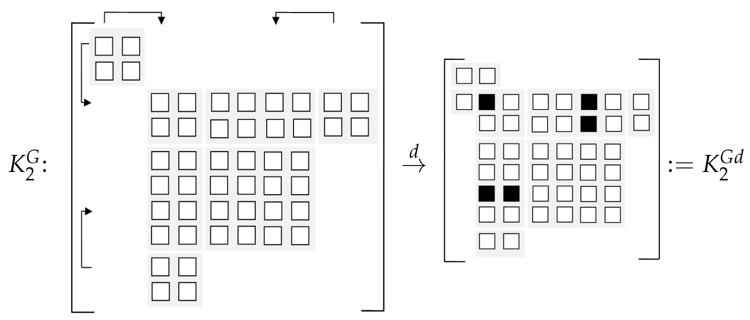
Analogously, there are eight block rows and block columns, each of the initial size $m^a\times m^a$ in $K_2^A$. The deflation process simultaneously adds the seventh column and row subblocks to the third column and row subblocks, respectively. Then the first column sub-block of the upper right $K_1^A$ and the first row sub-block of the lower-left $K_1^A$ overlap with the first column sub-block of $K_1^{AGH}$ and the first row sub-block of ${\left(K_1^{A^{\top }GH}\right)}^{\top }$, respectively, completing the deflation of $K_2^{Ad}$.

The whole process is described in Figure 1 and Figure 2 where each small square is of size $m^a\times m^a$ and each block with gray background represents the non-zero component in $K_2^G$ and $K_2^A$. The little white squares in $K_2^{Gd}$ and $K_2^{Ad}$ inherit from the originally undeflated submatrices and the little black squares in $K_2^{Gd}$ and $K_2^{Ad}$ represent the submatrices after summation.

Figure 1. The deflation process of $K_2^G$ (or $K_2^H$).

Figure 2. The deflation process of $K_2^A$.

Case for $k\ge 3$.

After the $(k-1)$-th deflation, the deflated matrices $L_{k-1}^{Gd}$, $L_{1,k-1}^{Ad}$, $L_{k-1}^{Hd}$ and $L_{2,k-1}^{Ad}$ are denoted by $L_{k-1}^G$, $L_{1,k-1}^A$, $L_{k-1}^H$ and $L_{2,k-1}^A$ for simplicity. Now there are $m_{k-1}^g-(k-1)m^a$ (or $m_{k-1}^h-(k-1)m^a$) columns in $L_{k-1}^G$ and $L_{1,k-1}^A$ (or $L_{k-1}^H$ and $L_{2,k-1}^A$) and $m_{k-1}^{a_2}-m^a$ (or $m_{k-1}^{a_1}-m^a$) columns in $D_{k-1}^{AGHG}{L}_{2,k-1}^A$ and $D_{k-1}^{AGHG}{L}_{k-1}^H$ (or $D_{k-1}^{A^{\top }HGH}{L}_{1,k-1}^A$ and $D_{k-1}^{A^{\top }HGH}{L}_{k-1}^G$) that are identical. Then, one can remove columns of

$$\begin{array}{c}{L}_{k-1}^G(:,(k-2)m^a+1:m_{k-1}^g-m^a)\left(or{L}_{k-1}^H(:,(k-2)m^a+1:m_{k-1}^h-m^a)\right)\hfill \end{array}$$

and

$$D_{k-1}^{AGHG}{L}_{2,k-1}^A(:,1:m_{k-1}^{a_2}-m^a)\left(or{D}_{k-1}^{A^{\top }HGH}{L}_{1,k-1}^A(:,1:m_{k-1}^{a_1}-m^a)\right),$$

and keep the columns of

$$L_{1,k-1}^A(:,1:m_{k-1}^g-(k-1)m^a)\left(or{L}_{2,k-1}^A(:,1:m_{k-1}^h-(k-1)m^a)\right)$$

and

$$D_{k-1}^{AGHG}{L}_{k-1}^H(:,m_{k-1}^h-m_{k-1}^{a_2}+1:m_{k-1}^h-m^a)\left(or{D}_{k-1}^{A^{\top }HGH}{L}_{k-1}^G(:,m_{k-1}^g-m_{k-1}^{a_1}+1:m_{k-1}^g-m^a)\right)$$

in $L_k^G$ (A1) (or $L_k^H$ (A3)), respectively. So there are $k-1$ matrices, each of order $N\times m^a$, that are left in $L_{k-1}^G$ (or $L_{k-1}^H$), i.e., $D_0^{AGHG}{L}_{20}^A,D_1^{AGHG}{D}_0^{A^{\top }HG}{L}_{20}^A,\dots ,D_{k-2}^{AGHG}{\mathsf{\Pi }}_{i=0}^{k-3}{D}_i^{A^{\top }HG}{L}_{20}^A$ in (A1) (or $D_0^{A^{\top }HGH}{L}_{10}^A,D_1^{A^{\top }HGH}{D}_0^{AGH}{L}_{10}^A,\dots ,D_{k-2}^{A^{\top }HGH}{\mathsf{\Pi }}_{i=0}^{k-3}{D}_i^{AGH}{L}_{10}^A$ in (A3)) in Appendix B. Meanwhile, only one matrix of order $N\times m^a$ is left in $D_{k-1}^{AGHG}{L}_{2,k-1}^A$, (or $D_{k-1}^{A^{\top }HGH}{L}_{1,k-1}^A$), i.e., the last item $D_{k-1}^{AGHG}{\mathsf{\Pi }}_{i=k-2}^0{D}_i^{A^{\top }HG}{L}_{20}^A$ in (A1) (or $D_{k-1}^{A^{\top }HGH}{\mathsf{\Pi }}_{i=k-2}^0{D}_i^{AGH}{L}_{10}^A$ in (A3)) of Appendix B. We also take $L_3^G$ as an example to describe the above deflation more clearly in Appendix C.

To deflate $L_{1,k}^A$ ($L_{2,k}^A$), columns of

$$D_{k-1}^{AGH}{L}_{1,k-1}^A(:,1:m_{k-1}^{a_1}-m^a)\left(\mathrm{or}{D}_{k-1}^{A^{\top }HG}{L}_{2,k-1}^A(:,1:m_{k-1}^{a_2}-m^a)\right)$$

are removed but the columns of

$$D_{k-1}^{AGH}{L}_{k-1}^G(:,m_{k-1}^g-m_{k-1}^{a_1}+1:m_{k-1}^g-m^a)\left(\mathrm{or}{D}_{k-1}^{A^{\top }HG}{L}_{k-1}^H(:,m_{k-1}^h-m_{k-1}^{a_2}+1:m_{k-1}^h-m^a)\right)$$

are retained in $L_{1,k}^A$ (or $L_{2,k}^A$). So only one matrix of order $N\times m^a$ is left in $D_{k-1}^{AGH}{L}_{1,k-1}^A$ (or $D_{k-1}^{A^{\top }HG}{L}_{2,k-1}^A$), i.e., the last item ${\mathsf{\Pi }}_{i=k-1}^0{D}_i^{AGH}{L}_{10}^A$ in (A2) (or ${\mathsf{\Pi }}_{i=k-1}^0{D}_i^{A^{\top }HG}{L}_{20}^A$ in (A4)) of Appendix B. Note that the low-rank factors in the $(k-1)$-th iteration are the ones after deflation, truncation and compression, deleting the superscript “d” for the simplicity. We take $L_{13}^A$ as an example to describe the above deflation more clearly in Appendix D.

Correspondingly, the kernel matrices $K_k^G$, $K_k^H$, and $K_k^A$ are deflated according to their low-rank factors. Here, we describe the deflation of $K_k^G$ and that of $K_k^H$ is essentially the same. By recalling the place of non-zero sub-matrices (the block with gray background in Figure 3) of $K_k^G$ in (21), the deflation process essentially adds $K_{k-1}^G((k-2)m^a+1:m_{k-1}^g-m^a,$$(k-2)m^a+1:m_{k-1}^g-m^a)$ to $K_{k-1}^{AGHG{A}^{\top }}(1:m_{k-1}^g-(k-1)m^a,1:m_{k-1}^g-(k-1)m^a)$, columns $K_{k-1}^A(:,1:m_{k-1}^{a_2}-m^a)$ to $K_{k-1}^{AGHG}(:,m_{k-1}^g+m_{k-1}^h-m_{k-1}^{a_2}+1:m_{k-1}^g+m_{k-1}^h-m^a)$ and rows ${\left(K_{k-1}^A\right)}^{\top }(1:m_{k-1}^{a_2}-m^a,:)$ to ${\left(K_{k-1}^{AGHG}\right)}^{\top }(m_{k-1}^g+m_{k-1}^h-m_{k-1}^{a_2}+1:m_{k-1}^g+m_{k-1}^h-m^a,:)$, respectively. See Figure 3 for illustration.

Figure 3. The deflation process of $K_k^G$ (or $K_k^H$).

Similarly, by recalling the positions of non-zero matrices (the block with gray background in Figure 4) of $K_k^A$ in (23), the deflation process will add columns $K_{k-1}^A(:,1:m_{k-1}^{a_2}-m^a)$ to columns $K_{k-1}^{AHG}(:,m_{k-1}^h-m_{k-1}^{a_2}+1:m_{k-1}^h-m^a)$ and rows $K_{k-1}^A(1:m_{k-1}^{a_1}-m^a,:)$ to rows ${\left(K_{k-1}^{A^{\top }GH}\right)}^{\top }(m_{k-1}^g-m_{k-1}^{a_1}+1:m_{k-1}^g-m^a,:)$. See Figure 4 for illustration.

Figure 4. The deflation process of $K_k^A$.

4. Partial Truncation and Compression

Although the deflation of the low-rank factors and kernels in the last section can reduce dimensional growth, the exponential increment of the undeflated part is still rapid, making large-scale computation and storage infeasible. Conventionally, one efficient way to shrink the column number of low-rank factors is by truncation and compression (TC) [17,18], which, unfortunately, is hard to be applied to our case due to the following two main obstacles.

• Direct application of TC to $L_k^{Hd}$, $L_k^{Gd}$, $L_{1,k}^{Ad}$, $L_{2,k}^{Ad}$, and their corresponding kernels $K_k^{Hd}$, $K_k^{Gd}$ and $K_k^{Ad}$ at the k-th step will require four QR decompositions, resulting in a relatively high computational complexity and CPU consumption.
• The TC process applied to the whole low-rank factors at current step breaks up the implicit structure, causing the deflation to be unrealized in the next iteration.

In this section, we will instead present a technique of partial truncation and compression (PTC) to overcome the above difficulties. Our PTC only requires two QR decompositions of the exponentially increasing (not the entire) parts of low-rank factors, keeping the successive deflation for subsequent iterations.

PTC for low-rank factors. Recall the deflated forms (A1) and (A3) in Appendix B. $L_k^{Gd}$ and $L_k^{Hd}$ can be divided to three parts

$$\begin{array}{c}{L}_k^{Gd}=[L_k^{Gd}\left(1\right),L_k^{Gd}\left(2\right),L_k^{Gd}\left(3\right)]\hfill \\ L_k^{Hd}=[L_k^{Hd}\left(1\right),L_k^{Hd}\left(2\right),L_k^{Hd}\left(3\right)].\hfill \end{array}$$

The number of columns in

$$\begin{array}{c}{L}_k^{Gd}\left(1\right):=[D_0^{AGHG}{L}_{20}^A,D_1^{AGHG}{D}_0^{A^{\top }GH}{L}_{20}^A,\dots ,D_{k-2}^{AGHG}{\mathsf{\Pi }}_{i=k-3}^0{D}_i^{A^{\top }GH}{L}_{20}^A]\in {\mathbb{R}}^{N\times (k-1)m^a}\hfill \end{array}$$

and

$$\begin{array}{c}{L}_k^{Hd}\left(1\right):=[D_0^{A^{\top }HGH}{L}_{10}^A,D_1^{A^{\top }HGH}{D}_0^{A^{\top }GH}{L}_{10}^A,\dots ,D_{k-2}^{A^{\top }HGH}{\mathsf{\Pi }}_{i=k-3}^0{D}_i^{AGH}{L}_{10}^A]\in {\mathbb{R}}^{N\times (k-1)m^a}\hfill \end{array}$$

increases only linearly with k, and the last parts

$$\begin{array}{c}{L}_k^{Gd}\left(3\right):=D_{k-1}^{AGHG}{\mathsf{\Pi }}_{i=k-2}^0{D}_i^{A^{\top }GH}{L}_{20}^A\in {\mathbb{R}}^{N\times m^a}\hfill \end{array}$$

and

$$\begin{array}{c}{L}_k^{Hd}\left(3\right):=D_{k-1}^{A^{\top }HGH}{\mathsf{\Pi }}_{i=k-2}^0{D}_i^{AGH}{L}_{10}^A\in {\mathbb{R}}^{N\times m^a}\hfill \end{array}$$

are always of size $N\times m^a$. So we only truncate and compress the dominantly growing parts

$$\begin{array}{c}{L}_k^{Gd}\left(2\right):=[L_{1,k-1}^A,D_{k-1}^{AGH}{L}_{k-1}^G,D_{k-1}^{AGHG}{L}_{k-1}^H]\hfill \end{array}$$

and

$$\begin{array}{c}{L}_k^{Hd}\left(2\right):=[L_{2,k-1}^A,D^{A^{\top }HG}{L}_{k-1}^H,D_{k-1}^{A^{\top }HGH}{L}_{k-1}^G]\hfill \end{array}$$

by orthogonalization. Consider the QR decompositions with column pivoting of

$$\begin{array}{cc}\hfill & L_k^{Gd}\left(2\right)P_k^G=\left[Q_k^G{\tilde{Q}}_k^G\right]\left[\begin{array}{cc}{U}_{k,1}^G& U_{k,2}^G\\ 0& {\tilde{U}}_k^G\end{array}\right],\parallel {\tilde{U}}_k^G\parallel <u_0^g{\tau }_g,\hfill \\ \hfill & L_k^{Hd}\left(2\right)P_k^H=\left[Q_k^H{\tilde{Q}}_k^H\right]\left[\begin{array}{cc}{U}_{k,1}^H& U_{k,2}^H\\ 0& {\tilde{U}}_k^H\end{array}\right],\parallel {\tilde{U}}_k^H\parallel <u_0^h{\tau }_h,\hfill \end{array}$$

(32)

where $P_k^G$ and $P_k^H$ are permutation matrices such that the diagonal elements of $\left[\begin{array}{cc}{U}_{k,1}^J& U_{k,2}^J\\ 0& {\tilde{U}}_k^J\end{array}\right]$ ($J=G$ or H) are decreasing in absolute value, $u_0^g=\parallel U_{0,1}^G\parallel$, $u_0^h=\parallel U_{0,1}^H\parallel$ and ${\tau }_g$ and ${\tau }_h$ are some small tolerances controlling PTC of $L_k^{Gd}\left(2\right)$ and $L_k^{Hd}\left(2\right)$, respectively, $m_k^{g\left(2\right)}$ and $m_k^{h\left(2\right)}$ are the respective column numbers of $L_k^G\left(2\right)$ and $L_k^H\left(2\right)$ bounded above by some given $m_{max}$. Then their ranks satisfy

$$r_k^g:=\mathrm{rank}\left(L_k^G\left(2\right)\right)\le m_k^{g\left(2\right)}\le m_{max},r_k^h:=\mathrm{rank}\left(L_k^H\left(2\right)\right)\le m_k^{h\left(2\right)}\le m_{max}$$

with $m_{max}\ll N$. Furthermore, $Q_k^G\in {\mathbb{R}}^{N\times r_k^g}$ and $Q_k^H\in {\mathbb{R}}^{N\times r_k^h}$ are orthonormal and $U_k^G=\left[U_{k,1}^G{U}_{k,2}^G\right]\in {\mathbb{R}}^{r_k^g\times m_{k-1}^{hga}}$ and $U_k^H=\left[U_{k,1}^H{U}_{k,2}^H\right]\in {\mathbb{R}}^{r_k^h\times m_{k-1}^{hga}}$ are full-rank with $m_{k-1}^{hga}=m_{k-1}^h+m_{k-1}^g+m_{k-1}^a$. Then $L_k^{Gd}$ and $L_k^{Hd}$ can be truncated and reorganized as

$$\begin{array}{c}{L}_k^{Gdt}=[L_k^{Gd}\left(1\right),Q_k^G,L_k^{Gd}\left(3\right)]:=[L_k^{Gdt}\left(1\right),L_k^{Gdt}\left(2\right),L_k^{Gdt}\left(3\right)]\in {\mathbb{R}}^{N\times m_k^g},\hfill \\ L_k^{Hdt}=[L_k^{Hd}\left(1\right),Q_k^H,L_k^{Hd}\left(3\right)]:=[L_k^{Hdt}\left(1\right),L_k^{Hdt}\left(2\right),L_k^{Hdt}\left(3\right)]\in {\mathbb{R}}^{N\times m_k^h}\hfill \end{array}$$

(33)

with $m_k^g=r_k^g+k{m}^a$ and $m_k^h=r_k^h+k{m}^a$.

Similarly, recalling the deflated forms in (A2) and (A4) in Appendix B, $L_{1,k}^{Ad}$ and $L_{2,k}^{Ad}$ are also divided into two parts,

$$\begin{array}{c}{L}_{1,k}^{Ad}=[L_{1,k}^{Ad}\left(1\right),L_{1,k}^{Ad}(2)]and{L}_{2,k}^{Ad}=[L_{2,k}^{Ad}\left(1\right),L_{2,k}^{Ad}\left(2\right)]\hfill \end{array}$$

with

$$\begin{array}{c}{L}_{1,k}^{Ad}\left(1\right)=L_k^{Gd}\left(2\right),L_{1,k}^{Ad}\left(2\right)={\mathsf{\Pi }}_{i=k-1}^0{D}_i^{AGH}{L}_{10}^A,\hfill \\ L_{2,k}^{Ad}\left(1\right)=L_k^{Hd}\left(2\right),L_{2,k}^{Ad}\left(2\right)={\mathsf{\Pi }}_{i=k-1}^0{D}_i^{A^{\top }HG}{L}_{20}^A.\hfill \end{array}$$

Since $L_k^{Gd}\left(2\right)$ and $L_k^{Hd}\left(2\right)$ have been compressed to $Q_k^G$ and $Q_k^H$, respectively, one has the truncated and compressed factors

$$\begin{array}{c}{L}_{1,k}^{Adt}=[Q_k^G,L_{1,k}^{Ad}\left(2\right)]=[L_{1,k}^{Adt}\left(1\right),L_{1,k}^{Adt}\left(2\right)]\in {\mathbb{R}}^{N\times m_k^{a_1}},\hfill \\ L_{2,k}^{Adt}=[Q_k^H,L_{2,k}^{Ad}\left(2\right)]=[L_{2,k}^{Adt}\left(1\right),L_{2,k}^{Adt}\left(2\right)]\in {\mathbb{R}}^{N\times m_k^{a_2}}\hfill \end{array}$$

(34)

with $m_k^{a_1}=r_k^g+m^a$ and $m_k^{a_2}=r_k^h+m^a$, finishing the PTC process for the low-rank factors in the k-th iteration.

It is worth noting that the above PTC process can proceed to the next iteration. In fact, one has

$$\begin{array}{c}{L}_{k+1}^G=[L_k^{Gdt},L_{1,k}^{Adt},D_k^{AGH}{L}_k^{Gdt},D_k^{AGHG}{L}_k^{Hdt},D_{k+1}^{AGHG}{L}_{2,k}^{Adt}],\hfill \\ L_{k+1}^H=[L_k^{Hdt},L_{2,k}^{Adt},D_k^{A^{\top }HG}{L}_k^{Hdt},D_k^{A^{\top }HGH}{L}_k^{Gdt},D_k^{A^{\top }HGH}{L}_{1,k}^{Adt}]\hfill \end{array}$$

after the k-th PTC. As $L_{1,k}^{Adt}\left(1\right)$ is equal to $L_k^{Gdt}\left(2\right)$ and $L_{2,k}^{Adt}\left(1\right)$ is equal to $L_k^{Hdt}\left(2\right)$, one can deflate $L_{k+1}^G$ and $L_{k+1}^H$ to

$$\begin{array}{c}{L}_{k+1}^{Gd}=[L_{k+1}^{Gd}\left(1\right),L_{k+1}^{Gd}\left(2\right),L_{k+1}^{Gd}\left(3\right)],L_{k+1}^{Hd}=[L_{k+1}^{Hd}\left(1\right),L_{k+1}^{Hd}\left(2\right),L_{k+1}^{Hd}\left(3\right)]\end{array}$$

with

$$\begin{array}{c}{L}_{k+1}^{Gd}\left(1\right)=[L_k^{Gdt}\left(1\right),L_k^{Gdt}\left(3\right)],L_{k+1}^{Hd}\left(1\right)=[L_k^{Hdt}\left(1\right),L_k^{Hdt}\left(3\right)],\\ L_{k+1}^{Gd}\left(2\right)=[L_{1,k}^{Adt},D_k^{AGH}{L}_k^{Gdt},D_k^{AGHG}{L}_k^{Hdt}],L_{k+1}^{Hd}\left(2\right)=[L_{2,k}^{Adt},D_k^{A^{\top }HG}{L}_k^{Hdt},D_k^{A^{\top }HGH}{L}_k^{Gdt}],\\ L_{k+1}^{Gd}\left(3\right)=D_k^{AGHG}{L}_{2,k}^{Adt}\left(2\right),L_{k+1}^{Hd}\left(3\right)=D_k^{A^{\top }HGH}{L}_{1,k}^{Adt}\left(2\right).\end{array}$$

Applying PTC to $L_{k+1}^{Gd}\left(2\right)$ and $L_{k+1}^{Hd}\left(2\right)$, respectively, again, one has

$$\begin{array}{c}{L}_{k+1}^{Gdt}=[L_{k+1}^{Gd}\left(1\right),Q_{k+1}^G{L}_{k+1}^{Gd}\left(3\right)]:=[L_{k+1}^{Gdt}\left(1\right),L_{k+1}^{Gdt}\left(2\right),L_{k+1}^{Gdt}\left(3\right)],\hfill \\ L_{k+1}^{Hdt}=[L_{k+1}^{Hd}\left(1\right),Q_{k+1}^H,L_{k+1}^{Hd}\left(3\right)]:=[L_{k+1}^{Hdt}\left(1\right),L_{k+1}^{Hdt}\left(2\right),L_{k+1}^{Hdt}\left(3\right)],\hfill \end{array}$$

(35)

where $Q_{k+1}^G\in {\mathbb{R}}^{N\times r_{k+1}^g}$ and $Q_{k+1}^H\in {\mathbb{R}}^{N\times r_{k+1}^h}$ are unitary matrices from QR decomposition and the PTC in the $(k+1)$-th iteration is completed.

PTC for kernels. Define matrices

$$\begin{array}{c}{\hat{U}}_{1,k}^A=U_k^G\oplus I_{m^a},{\hat{U}}_k^G=I_{(k-1)m^a}\oplus U_k^G\oplus I_{m^a},\hfill \\ {\hat{U}}_{2,k}^A=U_k^H\oplus I_{m^a},{\hat{U}}_k^H=I_{(k-1)m^a}\oplus U_k^H\oplus I_{m^a},\hfill \end{array}$$

with $U_k^G$ and $U_k^H$ in (32). Then the truncated and compressed kernels are

$$\begin{array}{c}{K}_k^{Gdt}:={\hat{U}}_k^G{K}_k^{Gd}{\left({\hat{U}}_k^G\right)}^{\top }\in {\mathbb{R}}^{m_k^g\times m_k^g},\hfill \\ K_k^{Hdt}:={\hat{U}}_k^H{K}_k^{Hd}{\left({\hat{U}}_k^H\right)}^{\top }\in {\mathbb{R}}^{m_k^h\times m_k^h},\hfill \\ K_k^{Adt}:={\hat{U}}_{1,k}^A{K}_k^{Hd}{\left({\hat{U}}_{2,k}^A\right)}^{\top }\in {\mathbb{R}}^{m_k^g\times m_k^h}.\hfill \end{array}$$

(36)

To eliminate items less than $O\left({\tau }_g\right)$ and $O\left({\tau }_h\right)$ in the low-rank factors and kernels, an additional monitoring step is imposed after the PTC process. Specifically, the last item $D_{k-2}^{AGHG}{\mathsf{\Pi }}_{i=k-3}^0{D}_i^{A^{\top }GH}{L}_{20}^A$ in $L_k^{Gdt}$ (or $D_{k-2}^{A^{\top }HGH}{\mathsf{\Pi }}_{i=k-3}^0{D}_i^{AGH}{L}_{10}^A$ in $L_k^{Hdt}$) will be discarded if its norm is less than $O\left({\tau }_g\right)$ (or $O\left({\tau }_h\right)$). Similarly, ${\mathsf{\Pi }}_{i=k-1}^0{D}_i^{AGH}{L}_{10}^A$ in $L_{1,k}^{Ad}\left(2\right)$ (or ${\mathsf{\Pi }}_{i=k-1}^0{D}_i^{A^{\top }HG}{L}_{20}^A$ in $L_{2,k}^{Ad}\left(2\right)$) will be abandoned if its norm is less than $O\left({\tau }_g\right)$ (or $O\left({\tau }_h\right)$). In this way, the growth of column dimension in the low-rank factors $L_k^{Gdt}$, $L_k^{Hdt}$, $L_{1,k}^{Adt}$ and $L_{2,k}^{Adt}$, as well as the kernels $K_k^{Gdt}$, $K_k^{Hdt}$, $K_k^{Adt}$, will be controlled efficiently while sacrificing a hopefully negligible bit of accuracy. Additionally, their sizes after PTC will be further restricted by setting a reasonable upper bound $m_{max}$.

5. Algorithm and Implementation

5.1. Computation of Residuals

The computation of relative residuals, such as $r_{rel}=|\mathcal{D}\left(H_k\right)|/|\mathcal{D}\left(H_0\right)|$, is commonly used in the context of solving the DARE using SDA, as mentioned in [4]. Typically, the FSDA algorithm is designed to stop when the relative residual is sufficiently small, which guarantees that the approximated solution $H_k$ is close to the exact solution of the DARE [35]. However, computing $r_{rel}$ directly can be computationally expensive due to the high rank of $H_k$ and $G_k$. To overcome this difficulty, the residual is divided into two parts, the banded part and the low-ranked part, under the assumptions of Equations (4) and (5). The residual for the banded part can be computed relatively easily and serves as a pre-termination condition, followed by the termination of the entire FSDA algorithm based on the residual for the low-ranked part.

5.1.1. Residual for the Banded Part

Define

$$\begin{array}{c}{\tilde{D}}_k^{HG}={(I+D_k^H{D}_0^G)}^{-1},{\tilde{D}}_k^{HGH}={\tilde{D}}_k^{HG}{D}_k^H,{\tilde{D}}_k^{GHG}=D_0^G{\tilde{D}}_k^{HG}\end{array}$$

and

$$\begin{array}{c}{\tilde{K}}_k^H={(I+K_k^H{\left(L_k^H\right)}^{\top }{\tilde{D}}_k^{GHG}{L}_k^H)}^{-1}{K}_k^H.\end{array}$$

With the current approximated solution $H_k=D_k^H+L_k^H{K}_k^H{\left(L_k^H\right)}^{\top }$, the residual for DARE (3) is

$$\begin{array}{cc}\hfill \mathcal{D}\left(H_k\right)& =-H_k+A^{\top }\left({\tilde{D}}_k^{HGH}+{\tilde{D}}_k^{HG}{L}_k^H{\tilde{K}}_k^H{\left({\tilde{D}}_k^{HG}{L}_k^H\right)}^{\top }\right)A+H\hfill \\ & :=D_k^R+L_k^R{K}_k^R{\left(L_k^R\right)}^{\top },\hfill \end{array}$$

where the banded part, the low-rank part and the kernel are

$$D_k^R=D_0^H-D_k^H+{\left(D_0^A\right)}^{\top }{D}_k^H{(I+D_0^G{D}_k^H)}^{-1}{D}_0^A,$$

$$L_k^R=[L_{20}^A,{\left(D_0^A\right)}^{\top }{\tilde{D}}_k^{HGH}{L}_{10}^A,{\left(D_0^A\right)}^{\top }{\tilde{D}}_k^{HG}{L}_k^H,L_k^H],$$

$$K_k^R=\begin{array}{cc}\hfill \begin{array}{c}\hfill m^a{m}^a{m}_k^h{m}_k^h\end{array}& \\ \hfill \left[\begin{array}{cccc}{\tilde{K}}_k^{A^{\top }HGHA}& I_{m^a}& {\tilde{K}}_k^{A^{\top }HG}& 0\\ I_{m^a}& 0& 0& 0\\ {\left({\tilde{K}}_k^{A^{\top }HG}\right)}^{\top }& 0& {\tilde{K}}_k^H& 0\\ 0& 0& 0& -K_k^H\end{array}\right]& \hfill \begin{array}{c}{m}^a\hfill \\ m^a\hfill \\ m_k^h\hfill \\ m_k^h\hfill \end{array}\end{array}$$

(37)

respectively, and

$${\tilde{K}}_k^{A^{\top }HG}={\left(L_{10}^A\right)}^{\top }{\tilde{D}}_k^{HG}{L}_k^H·{\tilde{K}}_k^H,$$

$${\tilde{K}}_k^{A^{\top }HGHA}={\left(L_{10}^A\right)}^{\top }{\tilde{D}}_k^{HGH}{L}_{10}^A+{\tilde{K}}_k^{A^{\top }HG}·{\left({\left(L_{10}^A\right)}^{\top }{\tilde{D}}_k^{HG}{L}_k^H\right)}^{\top }.$$

It is not difficult to see that the main flop counts in the kernel $K_k^R$ lie in forming matrices

$${\left(L_{10}^A\right)}^{\top }{\tilde{D}}_k^{HGH}{L}_{10}^A,{\left(L_{10}^A\right)}^{\top }{\tilde{D}}_k^{HG}{L}_k^H,{\left(L_k^H\right)}^{\top }{\tilde{D}}_k^{GHG}{L}_k^H.$$

(38)

To avoid calculating them in each iteration, we first verify if

$$\mathrm{B}\_\mathrm{R}\mathrm{R}\mathrm{e}\mathrm{s}=\frac{\parallel D_k^R\parallel }{|{\overline{D}}_0^R|+\parallel L_0^R{\parallel }^2\parallel K_0^R\parallel }\le {ϵ}_b$$

(39)

with $|{\overline{D}}_0^R|=\parallel D_0^A{\parallel }_2^2\parallel D_0^H\parallel \parallel {(I+D_0^G{D}_0^H)}^{-1}{\parallel }_2$ and ${ϵ}_b$ being the band tolerance. Here, the norm ${\parallel ·\parallel }_2$ is the matrix spectral norm, which is not easy to compute and is replaced by $l_1$-matrix norm in practice. This is feasible as the residual of $\mathcal{D}\left(H_k\right)$ comes from two relatively independent parts, i.e., the banded part and the low-rank part.

5.1.2. Residual for the Low-Rank Part

When the pre-termination (39) is satisfied, matrices in (38) are then constructed, followed by the deflation, truncation, and compression of the low-rank factor $L_k^R$. Specifically, the columns $L_{20}^A(:,1:m^a)$ are removed and columns of $L_k^H(:,1:m^a)$ are kept such that $L_k^R$ is deflated to $L_k^{Rd}$, i.e.,

Let ${\hat{I}}_{m^a}=[I_{m^a},0,\dots 0]\in {\mathbb{R}}^{m^a\times m_k^h}$, ${\hat{K}}_k^{A^{\top }HG}=[{\left({\tilde{K}}_k^{A^{\top }HG}\right)}^{\top },0,\dots ,0]\in {\mathbb{R}}^{m_k^h\times m_k^h}$. The kernel $K_k^R$ in (37) is correspondingly deflated as

$$K_k^R\stackrel{d}{\to }\begin{array}{cc}\hfill \begin{array}{c}\hfill m^a{m}_k^h{m}_k^h\end{array}& \\ \hfill \left[\begin{array}{ccc}0& 0& {\hat{I}}_{m^a}\\ 0& {\tilde{K}}_k^H& {\hat{K}}_k^{A^{\top }HG}\\ {\left({\hat{I}}_{m^a}\right)}^{\top }& {\left({\hat{K}}_k^{A^{\top }HG}\right)}^{\top }& {\hat{K}}_k^{A^{\top }HGHA}\end{array}\right]& \hfill \begin{array}{c}{m}^a\hfill \\ m_k^h\hfill \\ m_k^h\hfill \end{array}\end{array}:=K_k^{Rd},$$

where all elements in ${\hat{K}}_k^{A^{\top }HGHA}$ are same to those in $K_k^H$ except ${\hat{K}}_k^{A^{\top }HGHA}(1:m^a,1:m^a)={\tilde{K}}_k^{A^{\top }HGHA}-K_k^H(1:m^a,1:m^a)$.

After deflation, the truncation and compression are applied to $L_k^{Rd}$ with QR decomposition

$$\begin{array}{c}\hfill L_k^{Rd}{P}_k^R=\left[Q_k^R{\tilde{Q}}_k^R\right]\left[\begin{array}{cc}{U}_{k,1}^R& U_{k,2}^R\\ 0& {\tilde{U}}_k^R\end{array}\right],\parallel {\tilde{U}}_k^R\parallel <u_0^r{\tau }_r,\end{array}$$

where $P_k^R$ is the permutation matrix such that the diagonal elements of $\left[\begin{array}{cc}{U}_{k,1}^R& U_{k,2}^R\\ 0& {\tilde{U}}_k^R\end{array}\right]$ are decreasing in absolute value, $u_0^r=\parallel U_{0,1}^R\parallel$ and ${\tau }_r$ is the given tolerance, $Q_k^R\in {\mathbb{R}}^{n\times r_k^r}$ is orthonormal and $U_k^R=\left[U_{k,1}^R{U}_{k,2}^R\right]\in {\mathbb{R}}^{r_k^r\times n_k}$ is full-ranked. Since $\parallel L_k^R{K}_k^R{\left(L_k^R\right)}^{\top }\parallel \approx \parallel U_k^R{K}_k^{Rd}{\left(U_k^R\right)}^{\top }\parallel$, the terminating condition of the whole algorithm is chosen to be

$$\mathrm{L}\mathrm{R}\_\mathrm{R}\mathrm{R}\mathrm{e}\mathrm{s}=\frac{\parallel U_k^R{K}_k^{Rd}{\left(U_k^R\right)}^{\top }\parallel }{|{\overline{D}}_0^R|+\parallel L_0^R{\parallel }^2\parallel K_0^R\parallel }\le {ϵ}_l$$

(40)

with ${ϵ}_l$ being the low-rank tolerance.

5.2. Algorithm and Operation Counts

The process of deflation and PTC together with the computation of residuals (39) and (40) are summarized in the FSDA Algorithm 1.

Algorithm 1 FSDA. Solve DAREs with high-ranked G and H

Inputs:  Banded matrices $D_0^A$, $D_0^G$, $D_0^H$, low-rank factors $L_{10}^A$, $L_{20}^A$, $L_0^G$, $L_0^H$, $K_0^G$, $K_0^H$, and the iterative tolerance $tol$; truncation tolerances ${\tau }_g$, ${\tau }_h$, ${\tau }_r$ and upper bound $m_{max}$; band tolerance ${ϵ}_b$ and low-rank tolerance ${ϵ}_l$. Outputs:  Banded matrix $D^H$, low-rank matrix $L^H$ and the kernel matrix $K^H$ with the stabilizing solution $X_s\approx D^H+L^H{K}^H{\left(L^H\right)}^{\top }$. Set $D_1^G=D_0^G+D_0^{AGHG}{\left(D_0^A\right)}^{\top }$, $D_1^H=D_0^H+D_0^{A^{\top }HGH}{D}_0^A$, $D_1^A=D_0^A{\left(D_0^{A^{\top }HG}\right)}^{\top }$ as in (9). Set $L_1^G=[L_{10}^A,D_0^{AGHG}{L}_{20}^A]$, $L_1^H=[L_{20}^A,D_0^{A^{\top }HGH}{L}_{10}^A]$, $L_{11}^A=[L_{10}^A,D_0^{AGH}{L}_{10}^A]$, $L_{21}^A=[L_{20}^A,D_0^{A^{\top }HG}{L}_{20}^A]$ as in (10). Set $K_1^G$, $K_1^H$, $K_1^A$ as in (11) and (12). For$k=2,\dots ,$ until convergence, do  Compute banded matrices $D_k^G$, $D_k^H$, $D_k^A$ as in (13).  Form components (18)–(20) and construct kernels $K_k^G$, $K_k^G$ and $K_k^G$ as in (21)–(23).  Deflate kernels $K_k^G\stackrel{d}{\to }{K}_k^{Gd}$, $K_k^H\stackrel{d}{\to }{K}_k^{Hd}$ and $K_k^A\stackrel{d}{\to }{K}_k^{Ad}$ in a way of Figure 3 and Figure 4.  Deflate the low-rank factors $L_k^G\stackrel{d}{\to }{L}_k^{Gd}$, $L_k^H\stackrel{d}{\to }{L}_k^{Hd}$, $L_{1,k}^A\stackrel{d}{\to }{L}_{1,k}^{Ad}$ and $L_{2,k}^A\stackrel{d}{\to }{L}_{2,k}^{Ad}$ as in (A1)–(A4).  Partially truncate and compress $L_k^{Gd}$ and $L_k^{Hd}$ as in (32) with accuracy $u_0^g{\tau }_g$, $u_0^g{\tau }_h$.  Construct compressed low-rank factors $L_k^{Gdt}$, $L_k^{Hdt}$, $L_{1,k}^{Adt}$ and $L_{2,k}^{Adt}$ as in (33)–(34).  Construct compressed kernels $K_k^{Gdt}$, $K_k^{Hdt}$ and $K_k^{Adt}$ as in (36).  Evaluate the residual of the banded part B_RRes in (39).  If B_RRes $<tol$, compute the residual of low-rank part LR_RRes in (40).   If LR_RRes $<tol$, break, end.  End (If);  $K_k^G:=K_k^{Gdt}$, $K_k^H:=K_k^{Hdt}$, $K_k^A:=K_k^{Adt}$.  $L_k^G:=L_k^{Gdt}$, $L_k^H:=L_k^{Hdt}$, $L_{1,k}^A:=L_{1,k}^{Adt}$, $L_{2,k}^A:=L_{2,k}^{Adt}$.  $k:=k+1$; End (For) Output $D_k^H=D^H$, $L_k^H=L^H$ and $K_k^H=K^H$.

Remark 3.

1. At each iteration, elements in the banded matrices $D_k^A$, $D_k^H$, and $D_k^G$ with an absolute value less than $tol=eps·max\{\parallel D^A\parallel ,\parallel D^G\parallel ,\parallel D^H\parallel \}$ are eliminated.

2. The deflation process involves merging selected rows and columns in the kernels $K_k^G$, $K_k^H$, and $K_k^A$ based on overlapping columns in the low-rank factors $L_k^G$, $L_k^H$, $L_{1,k}^A$, and $L_{2,k}^A$. This requires adding some columns and rows.

3. The PTC is applied to $L_k^{Gd}\left(2\right)$ and $L_k^{Hd}\left(2\right)$. The column numbers of $L_k^{Gd}\left(1\right)$ and $L_k^{Hd}\left(1\right)$ increase linearly with respect to $k,$ while those of $L_k^{Gd}\left(3\right)$ and $L_k^{Hd}\left(3\right)$ remain unchanged. Elements in $L_k^{Gd}\left(1\right)$, $L_k^{Hd}\left(1\right)$, $L_k^{Gd}\left(3\right)$, and $L_k^{Hd}\left(3\right)$ with an absolute value less than $tol$ are removed to minimize the column size of the low-rank factors.

To further analyze the complexity and the memory requirement of the FSDA, the bandwidth of $D_k^A$, $D_k^G$, and $D_k^H$ at each iteration are assumed to be $b_k^a$, $b_k^g$ and $b_k^h$ ($b_k^a,b_k^g,b_k^h\ll N$), respectively. We also set $b_k^{hg}=max\{b_k^h,b_k^g\}$, $b_k^{hga}=max\{b_k^h,b_k^g,b_k^a\}$, $m_k^a=max\{m_k^{a_1},m_k^{a_2}\}$, and $m_{k-1}^{hga}:=m_{k-1}^h+m_{k-1}^g+m_{k-1}^a$ for the convenience of counting flops. The table in Appendix E lists the time and memory requirement for different components in the k-th iteration of the FSDA, where the estimations are upper bounds due to the truncation errors ${\tau }_g$, ${\tau }_h$ and ${\tau }_r$.

6. Numerical Examples

In this section, we will demonstrate the effectiveness of the FSDA algorithm in computing the approximate solution of the DARE (3). The FSDA algorithm was implemented using MATLAB 2014a [38] on a 64-bit PC running Windows 10. The PC had a 3.0 GHz Intel Core i5 processor with 6 cores and 6 threads, 32GB RAM, and a machine unit round-off value of eps = $2.22\times {10}^{-16}$. The residual for the DARE was estimated using the upper bound formula

$${\tilde{r}}_k=\mathrm{B}\_\mathrm{R}\mathrm{R}\mathrm{e}\mathrm{s}+\mathrm{L}\mathrm{R}\_\mathrm{R}\mathrm{R}\mathrm{e}\mathrm{s},$$

where B_RRes in (39) and LR_RRes in (40) are the relative residuals for the banded part and the low-rank part, respectively. The tolerance values for truncation and compression were set to ${\tau }_g={\tau }_h={\tau }_r={10}^{-16}$, and the termination tolerance values were set to ${ϵ}_b={ϵ}_l={10}^{-11}$. We also tried $N·$eps as the tolerance value for ${\tau }_g$, ${\tau }_h$ and ${\tau }_r$ in our experiments, but found that it had no impact on the residual accuracy. The maximum permitted column number in the low-rank factors was set to $m_{max}=2200$. As a comparison, we also ran the ordinary SDA algorithm with hierarchical structure (i.e., HODLR) using the hm-toolbox (http://github.com/numpi/hm-toolbox, accessed on 1 June 2023) [39,40]. The SDA algorithm with hierarchical structure is referred to as SDA_HODLR in this paper. The derived relative residual for SDA_HODLR is denoted by ${\hat{r}}_k$. In our numerical experiments, the initial bandwidths of all banded matrices in Examples 1 and 3 were relatively small, while those in Example 2 were non-trivial.

Example 1.

The first example is of the medium scale, measuring the error between the true solution and the computed one. Given the constant$\theta =\sqrt{\eta +\frac{1}{\eta }-2\zeta }$, where ζ and η are positive numbers such that θ is real. Let $L_{10}^A=\theta e$ with e the random vector satisfying $e^{\top }e=1$, $L_{20}^A=L_{10}^A$, $D_0^A=\zeta I_{{}_N}$, then $A=D_0^A+L_{10}^A{\left(L_{20}^A\right)}^{\top }$. Set $G=D_0^G=I_{{}_N}$, $H=D_0^H=(\eta +\frac{1}{\eta })D_0^A-{\left(D_0^A\right)}^2-I_{{}_N}$. The solution of the DARE is of the form $X_s=D^X+L^X{\left(L^X\right)}^{\top }$ with $D^X=\eta D_0^A-I_{{}_N}$ and $L^X=\sqrt{\eta }{L}_{10}^A$.

It is not difficult to see that the solution $X_s$ is stabilizing since the spectral radius of ${(I_{{}_N}+G{X}_s)}^{-1}A$ is less than unity when $\eta >1$.

We first took $\zeta =1.2$ and $\eta =2$ to calculate B_RRes, followed by LR_RRes as well as the upper bound of residual of DARE ${\tilde{r}}_k$. In our implementations, the relative error between the approximated solution (denoted by $H_j$ when terminated at the j-th iteration) and the true stabilizing solution $X_s$ was evaluated, and the numerical results are presented in Table 1. It is seen that for different scales ($N=1000,3000,5000,7000$) FSDA was able to attain the prescribed banded accuracy in five iterations. Residuals LR_Res and ${\tilde{r}}_k$ were then evaluated, attaining the order $O\left({10}^{-16}\right)$. The relative error with the computational time being not included in the CPU time, also reflects that $H_5$ approximates the true solution very well. On the other hand, SDA_HODLR also attains the prescribed residual accuracy in five iterations, but cost more CPU time (in seconds).

Table 1. Residual and actual errors in Example 1.

		$\mathit{\zeta }=1.2$, $\mathit{\eta }=2.0$
$\mathit{N}$	1000	3000	5000	7000
		FSDA
	$4.39\times {10}^{-1}$	$4.41\times {10}^{-1}$	$4.42\times {10}^{-1}$	$4.42\times {10}^{-1}$
	$3.47\times {10}^{-2}$	$3.48\times {10}^{-2}$	$3.49\times {10}^{-2}$	$3.49\times {10}^{-2}$
B_RRes	$1.38\times {10}^{-4}$	$1.38\times {10}^{-4}$	$1.38\times {10}^{-4}$	$1.38\times {10}^{-4}$
	$2.10\times {10}^{-9}$	$2.11\times {10}^{-9}$	$2.11\times {10}^{-9}$	$2.11\times {10}^{-9}$
	$4.25\times {10}^{-16}$	$4.27\times {10}^{-16}$	$4.27\times {10}^{-16}$	$4.31\times {10}^{-16}$
LR_RRes	$2.09\times {10}^{-18}$	$2.27\times {10}^{-18}$	$4.04\times {10}^{-18}$	$3.28\times {10}^{-18}$
${\tilde{r}}_k$	$4.27\times {10}^{-16}$	$4.29\times {10}^{-16}$	$4.31\times {10}^{-16}$	$4.34\times {10}^{-16}$
$\parallel H_5-X_s\parallel /\parallel X_s\parallel$	$2.56\times {10}^{-16}$	$2.57\times {10}^{-16}$	$2.56\times {10}^{-16}$	$2.48\times {10}^{-16}$
CPU	0.04	0.09	0.22	0.48
		SDA_HODLR
	$4.44\times {10}^{-1}$	$4.44\times {10}^{-1}$	$4.44\times {10}^{-1}$	$4.44\times {10}^{-1}$
	$3.50\times {10}^{-2}$	$3.50\times {10}^{-2}$	$3.50\times {10}^{-2}$	$3.50\times {10}^{-2}$
${\hat{r}}_k$	$1.39\times {10}^{-4}$	$1.39\times {10}^{-4}$	$1.39\times {10}^{-4}$	$1.39\times {10}^{-4}$
	$2.12\times {10}^{-9}$	$2.12\times {10}^{-9}$	$2.12\times {10}^{-9}$	$2.12\times {10}^{-9}$
	$1.33\times {10}^{-15}$	$1.27\times {10}^{-15}$	$1.34\times {10}^{-15}$	$1.47\times {10}^{-15}$
CPU	1.17	19.93	76.67	186.61
		$\mathit{\zeta }=\mathbf{1}.\mathbf{0}$,$\mathit{\eta }=\mathbf{1.2}$
$\mathit{N}$	1000	3000	5000	7000
		FSDA
	$8.68\times {10}^{-1}$	$8.84\times {10}^{-1}$	$8.89\times {10}^{-1}$	$8.92\times {10}^{-1}$
	$6.06\times {10}^{-1}$	$6.18\times {10}^{-1}$	$6.21\times {10}^{-1}$	$6.23\times {10}^{-1}$
	$1.93\times {10}^{-1}$	$1.97\times {10}^{-1}$	$1.98\times {10}^{-1}$	$1.99\times {10}^{-1}$
B_RRes	$1.15\times {10}^{-2}$	$1.18\times {10}^{-2}$	$1.18\times {10}^{-2}$	$1.19\times {10}^{-2}$
	$3.40\times {10}^{-5}$	$3.47\times {10}^{-5}$	$3.49\times {10}^{-5}$	$3.50\times {10}^{-5}$
	$2.91\times {10}^{-10}$	$2.97\times {10}^{-10}$	$2.99\times {10}^{-10}$	$3.00\times {10}^{-10}$
	$8.22\times {10}^{-16}$	$8.38\times {10}^{-16}$	$8.43\times {10}^{-16}$	$8.46\times {10}^{-16}$
LR_RRes	$3.03\times {10}^{-17}$	$1.07\times {10}^{-17}$	$2.77\times {10}^{-17}$	$1.75\times {10}^{-17}$
${\tilde{r}}_k$	$8.52\times {10}^{-16}$	$8.48\times {10}^{-16}$	$8.70\times {10}^{-16}$	$8.63\times {10}^{-16}$
$\parallel H_7-X_s\parallel /\parallel X_s\parallel$	$4.23\times {10}^{-15}$	$5.04\times {10}^{-15}$	$4.94\times {10}^{-15}$	$4.98\times {10}^{-15}$
CPU	0.31	0.45	0.48	0.96
		SDA_HODLR
	$9.08\times {10}^{-1}$	$9.08\times {10}^{-1}$	$9.08\times {10}^{-1}$	$9.08\times {10}^{-1}$
	$6.34\times {10}^{-1}$	$6.34\times {10}^{-1}$	$6.34\times {10}^{-1}$	$6.34\times {10}^{-1}$
	$2.02\times {10}^{-1}$	$2.02\times {10}^{-1}$	$2.02\times {10}^{-1}$	$2.02\times {10}^{-1}$
${\hat{r}}_k$	$1.21\times {10}^{-2}$	$1.21\times {10}^{-2}$	$1.21\times {10}^{-2}$	$1.21\times {10}^{-2}$
	$3.56\times {10}^{-5}$	$3.56\times {10}^{-5}$	$3.56\times {10}^{-5}$	$3.56\times {10}^{-5}$
	$3.05\times {10}^{-10}$	$3.05\times {10}^{-10}$	$3.05\times {10}^{-10}$	$3.05\times {10}^{-10}$
	$4.75\times {10}^{-15}$	$4.62\times {10}^{-15}$	$4.97\times {10}^{-15}$	$5.52\times {10}^{-15}$
CPU	1.61	27.10	107.16	263.34

We then took $\eta =1.2$ to make the spectral radius of ${(I_{{}_N}+G{X}_s)}^{-1}A$ close to 1 and recorded the numerical performance of the FSDA with $\zeta =1.0$. It is seen from Table 1 that the FSDA costs seven iterations before termination, obtaining almost the same banded residual histories (B_RRes) for different N. As before, LR_RRes and ${\tilde{r}}_k$ were of $O\left({10}^{-17}\right)$ and $O\left({10}^{-16}\right)$, respectively, showing that $H_7$ is a good approximation to the true solution to DARE (3). The last relative error $\parallel H_7-X_s\parallel /\parallel X_s\parallel$ also validates this fact. Analogously, SDA_HODLR requires seven iterations to arrive at the residual level $O\left({10}^{-15}\right)$. It is also seen that the FSDA costs less CPU time than SDA_HODLR for all N.

Example 2.

Consider a generalized model of power system labelled by PI Sections 20–80 (https://sites.google.com/site/rommes/software, “S10PI_n1.mat” accessed on 1 June 2023). All transmission lines in the network are modelled by RLC ladder networks, of cascaded RLC PI-circuits [41]. The original band-plus-low-rank matrix A has a small scale of 528 (Figure 5) and is then extended to larger ones. Specifically, we extract the banded part $D_{\mathrm{ori}}^A$ of the bandwidth 217 from the original matrix $A_{\mathrm{ori}}$ and tile it along the diagonal direction for 20 times to obtain $D_0^A$. We then implement an SVD of the matrix $A_{\mathrm{ori}}-D_{\mathrm{ori}}^A$ to produce the singular value matrix ${\mathsf{\Sigma }}_A$ and the unitary matrices $U_A$ and $V_A$. The low-ranked parts $L_{10}^A$ and $L_{20}^A$ are then constructed by tiling $U_A(:,1:r_a)$ and $V_A(:,1:r_a)$ 20 times and multiplying ${\mathsf{\Sigma }}_A^{1/2}(1:r_a,1:r_a)$ from the right, respectively, where $r_a$ is the number of singular values in ${\mathsf{\Sigma }}_A$ less than ${10}^{-8}$. Let $F_1$ and $F_3$ be block diagonal matrices with each diagonal block the $3\times 3$ random matrix (generated by‘rand(3)’). Let $F_2$ and $F_4$ be also diagonal block matrices with the top left element a random number, the last diagonal block $2\times 2$ random matrix and others $3\times 3$ random matrices. Define matrices G and H as

$$G:=D_0^G=(R_g+R_g^{\top })/2+\xi I_N,H:=D_0^H=(R_h+R_h^{\top })/4+\xi I_N,$$

with $R_g=(F_1+I_N)(F_2+I_N)$, $R_h=(F_3+I_N)(F_4+I_N)$.

Figure 5. Structured matrix $A_{\mathrm{ori}}$ of size $528\times 528$ in Example 2.

We ran the FSDA with three different $\xi =0.11,1.0,3.0$, each conducting five random experiments. In all experiments, B_RRes and LR_RRes (in $log10$) were observed attaining the pre-terminating condition (39) and the terminating condition (40), respectively.

Figure 6 plots the obtained numerical results for five experiments, where Rk is the upper bound of the residual of the DARE, BRes and LRes are the absolute residuals of the banded part and the low-rank part (i.e., the numerators in B_RRes and LR_RRes), respectively. It is seen that the relative residual levels of LR_RRes and B_RRes (between ${10}^{-14}$ and ${10}^{-17}$) are lower than those of LRes and BRes (between ${10}^{-11}$ and ${10}^{-13}$) in all experiments. Particularly, the gap between them increases as $\xi$ becomes larger. On the other hand, the residual line of Rk is above the residual lines of B_RRes or LR_RRes, attaining the level between ${10}^{-15}$ and ${10}^{-16}$. This demonstrates that the FSDA can obtain a relatively high residual accuracy.

Figure 6. Residual of the banded part and the low-rank part for different $\xi$.

To clearly see the evolution of the bandwidth of the banded matrices and the dimensional increase in the low-rank factors for five iterations, we listed the history of bandwidths of $D_k^G$, $D_k^H$, and $D_k^A$ (denoted by $b_k^g$, $b_k^h$, and $b_k^a$, respectively) and the column numbers of $L_k^{Hdt}$ and $L_k^{Gdt}$ (denoted by $m_k^h$ and $m_k^g$, respectively) in Table 2, where the CPU row recorded the consumed CPU time in seconds. It is obviously seen that, for $\xi =0.11,1$, and 3, the FSDA requires 5, 4, and 3 iterations to reach the prescribed accuracy, respectively. Further experiments show that the required number of iterations, when terminated, will decrease as $\xi$ goes larger. Additionally, we see that bandwidths $b_k^g$ and $b_k^h$ rise much in the second iteration but keep almost unchanged for the remaining iterations. Nevertheless, $b_k^a$ decreases gradually after reaching the maximal value in the second iteration, which is consistent with the convergence of $D_k^A$ in Corollary 1. On the other hand, we see from $m_k^h$ and $m_k^g$ that the column numbers in the second iteration are about fourfold of those in the first iteration since the FSDA does not deflate the low-rank factors at the first iteration. However, the column numbers in the fifth iteration (if it exists) are less than twofold of those in the fourth iteration. This reflects that deflation and PTC are efficient in reducing the dimensions of low-rank factors. In our experiments, we also found that nearly half of the CPU time in the FSDA was consumed in forming ${(I_{{}_N}+D_k^H{D}_0^G)}^{-1}{D}_k^H$ in the pre-termination. However, such a time expense might decrease if the initial bandwidths $b_0^g$, $b_0^h$, and $b_0^a$ are narrow.

Table 2. CPU times and history of bandwidth of banded matrices and column numbers of low-rank factors in Example 2.

	1	2	3	4	5
	$\left[{\mathit{b}}_{\mathit{k}}^{\mathit{g}}{\mathit{b}}_{\mathit{k}}^{\mathit{h}}{\mathit{b}}_{\mathit{k}}^{\mathit{a}}{\mathit{m}}_{\mathit{k}}^{\mathit{h}}{\mathit{m}}_{\mathit{k}}^{\mathit{g}}\right]$	$\left[{\mathit{b}}_{\mathit{k}}^{\mathit{g}}{\mathit{b}}_{\mathit{k}}^{\mathit{h}}{\mathit{b}}_{\mathit{k}}^{\mathit{a}}{\mathit{m}}_{\mathit{k}}^{\mathit{h}}{\mathit{m}}_{\mathit{k}}^{\mathit{g}}\right]$	$\left[{\mathit{b}}_{\mathit{k}}^{\mathit{g}}{\mathit{b}}_{\mathit{k}}^{\mathit{h}}{\mathit{b}}_{\mathit{k}}^{\mathit{a}}{\mathit{m}}_{\mathit{k}}^{\mathit{h}}{\mathit{m}}_{\mathit{k}}^{\mathit{g}}\right]$	$\left[{\mathit{b}}_{\mathit{k}}^{\mathit{g}}{\mathit{b}}_{\mathit{k}}^{\mathit{h}}{\mathit{b}}_{\mathit{k}}^{\mathit{a}}{\mathit{m}}_{\mathit{k}}^{\mathit{h}}{\mathit{m}}_{\mathit{k}}^{\mathit{g}}\right]$	$\left[{\mathit{b}}_{\mathit{k}}^{\mathit{g}}{\mathit{b}}_{\mathit{k}}^{\mathit{h}}{\mathit{b}}_{\mathit{k}}^{\mathit{a}}{\mathit{m}}_{\mathit{k}}^{\mathit{h}}{\mathit{m}}_{\mathit{k}}^{\mathit{g}}\right]$
	[445 445 445 34 34]	[445 445 445 34 34]	[445 445 445 34 34]	[ 445 445 445 34 34]	[445 445 445 34 34]
	[979 980 981 126 132]	[982 982 1042 126 132]	[973 767 973 126 132]	[1047 1033 1051 126 132]	[998 998 997 126 132]
$\xi =0.11$	[981 980 980 474 484]	[981 980 980 474 481]	[973 767 748 480 492]	[1050 1047 1049 468 495]	[998 999 973 474 488]
	[981 980 768 1012 1020]	[981 980 768 1014 1018]	[973 767 674 1025 1032]	[1050 1042 1047 1096 1028]	[981 980 768 1011 1023]
	[981 980 519 1758 1767]	[981 980 522 1759 1771]	[973 767 493 1801 1812]	[1050 1042 983 1946 1853]	[981 980 525 1762 1773]
CPU	4443.63	4451.36	4456.96	4414.65	4457.14
	[445 445 445 34 34]	[445 445 445 34 34]	[445 445 445 34 34]	[ 445 445 445 34 34]	[445 445 445 34 34]
	[973 767 973 126 132]	[768 973 769 126 132]	[815 973 973 126 132]	[1033 996 1042 126 132]	[745 745 748 126 132]
$\xi =1$	[973 973 973 471 476]	[767 973 766 469 476]	[815 973 768 477 487]	[1042 1042 1042 479 490]	[753 980 732 474 488]
	[973 973 646 911 927]	[767 973 555 910 916]	[815 973 646 1007 1027]	[1042 1042 840 973 980]	[753 980 684 923 931]
CPU	4014.65	4025.74	3993.86	4107.84	4020.12
	[445 445 445 34 34]	[445 445 445 34 34]	[445 445 445 34 34]	[445 445 445 34 34]	[445 445 445 34 34]
$\xi =3.0$	[652 654 674 126 132]	[746 746 746 126 132]	[695 673 675 126 132]	[674 686 685 126 132]	[701 703 686 126 132]
	[652 654 519 448 453]	[746 746 650 466 475]	[695 673 614 449 454]	[674 686 658 447 454]	[701 703 651 448 455]
CPU	1797.39	1640.02	1803.23	1748.16	1695.01

To further compare numerical performances between the FSDA and SDA_HODLR for larger problems, we extended the original scale to N = 15,840, 21,120, 26,400 and 31,680 at $\xi =3.0$ and ran both algorithms until convergence. The results are listed in Table 3, where one can see that both the FSDA and SDA_HODLR (i.e., SDA_HD in the table) attain the prescribed residual accuracy within three iterations, and SDA_HODLR requires less CPU time than FSDA does. However, there seems a strong tendency that the FSDA will outperform the SDA_HODLR on CPU time for larger problems, as the CPU time of the SDA_HODLR appears to surge at N = 26,400 and SDA_HODLR used up memory at N = 31,680 without producing any numerical results (denoted by “—”). The symbols “*” in the SDA_HODLR column represent no related records for bandwidth and column number of the low-rank factors.

Table 3. Numerical results for FSDA and SDA_HODLR in Example 2 at $\xi =3.0$. The symbol * stands for no related records.

N	15,840		21,120		26,400		31,680
	FSDA	SDA_HD	FSDA	SDA_HD	FSDA	SDA_HD	FSDA	SDA_HD
$b_k^g$	[445 695 695]	*	[445 736 736]	*	[445 723 723]	*	[445 652 652]	*
$b_k^h$	[445 673 673]	*	[445 745 745]	*	[445 737 737]	*	[445 654 654]	*
$b_k^a$	[445 675 614]	*	[445 745 674]	*	[445 738 653]	*	[445 674 619]	*
$m_k^h$	[34 126 448]	*	[34 126 469]	*	[34 126 460]	*	[34 126 444]	*
$m_k^g$	[34 132 453]	*	[34 132 476]	*	[34 132 469]	*	[34 132 454]	*
IT.	3	3	3	3	3	3	3	—
RES.	7.83 $\times {10}^{-17}$	1.44 $\times {10}^{-15}$	7.27 $\times {10}^{-17}$	1.70 $\times {10}^{-15}$	8.04 $\times {10}^{-17}$	1.74 $\times {10}^{-15}$	5.96 $\times {10}^{-15}$	—
CPU	6740.54	1285.31	13,037.43	3701.43	18,154.14	17,653.63	21,618.03	—

We further modified this example to have a simpler banded part to test both algorithms. Specifically, the relatively data-concentrated banded part of bandwidth 3 is extracted and tiled along the diagonal direction for 20 times to form $D_0^A$. As before, an SVD is imposed on the rest matrix to construct the low-ranked parts $L_{10}^A$ and $L_{20}^A$ after tiling the derived unitary matrices 20 times and multiplying ${\mathsf{\Sigma }}_A^{1/2}(1:r_a,1:r_a)$ from the right. We still selected $\xi =3.0$ and ran both the FSDA and SDA_HODLR at scales N = 15,840, 21,120, 26,400 and 31,680 again. The obtained results are recorded in Table 4, where it is readily seen that the FSDA outperforms the SDA_HODLR on CPU time. Once again, the SDA_HODLR ran out of memory for the case N = 31,680.

Table 4. Numerical results for FSDA and SDA_HODLR in relatively simpler banded part of Example 2 at $\xi =3.0$. The symbol * stands for no related records.

N	15,840		21,120		26,400		31,680
	FSDA	SDA_HD	FSDA	SDA_HD	FSDA	SDA_HD	FSDA	SDA_HD
$b_k^g$	[31 31 31]	*	[36 37 37]	*	[38 39 39]	*	[34 37 37]	*
$b_k^h$	[28 30 30]	*	[34 36 36]	*	[38 40 40]	*	[36 39 39]	*
$b_k^a$	[28 31 28]	*	[36 38 34]	*	[38 42 38]	*	[34 40 35]	*
$m_k^h$	[48 280 628]	*	[48 286 647]	*	[48 287 651]	*	[48 285 647]	*
$m_k^g$	[48 281 628]	*	[48 285 645]	*	[48 287 650]	*	[48 287 650]	*
IT.	3	3	3	3	3	3	3	—
RES.	5.95 $\times {10}^{-17}$	2.09 $\times {10}^{-15}$	3.46 $\times {10}^{-16}$	1.81 $\times {10}^{-15}$	8.49 $\times {10}^{-16}$	3.05 $\times {10}^{-15}$	9.93 $\times {10}^{-17}$	—
CPU	133.71	1255.06	218.07	3744.06	288.53	15,508.81	344.18	—

Example 3.

This example is an extension of small-scale electric power systems networks to a large-scale one which is used for signal stability analysis [19,20,21]. The corresponding matrix $A_{\mathrm{ori}}$ is from the power system of New England (https://sites.google.com/site/rommes/software, “ww_36_pemc_36.mat”, accessed on 1 June 2023). Figure 7 presents the original structure of the matrix A of order 66. We properly modified elements $A_{\mathrm{ori}}(32,28)=-36.4687$, $A_{\mathrm{ori}}(32,29)=-37.922$, $A_{\mathrm{ori}}(46,42)=-33.0033$; $A_{\mathrm{ori}}(46,43)=-76.8277$, $A_{\mathrm{ori}}(60,56)=-83.0405$, $A_{\mathrm{ori}}(60,57)=-73.9947$, $A_{\mathrm{ori}}(60,59)=-34.0478$. Then the banded part $D_{\mathrm{ori}}^A$ is extracted from blocks $A_{\mathrm{ori}}$(1:6, 1:6), $A_{\mathrm{ori}}$(7:13, 7:13), $A_{\mathrm{ori}}$(14:20, 14:20), $A_{\mathrm{ori}}$(21:27, 21:27), $A_{\mathrm{ori}}$(28:34, 28:34), $A_{\mathrm{ori}}$(35:41, 35:41), $A_{\mathrm{ori}}$(42:48, 42:48), $A_{\mathrm{ori}}$(49:55, 49:55), $A_{\mathrm{ori}}$(56:62, 56:62), and $A_{\mathrm{ori}}$(63:66, 63:66), admitting the bandwidth of 4. After tiling $D_{\mathrm{ori}}^A$ 200, 400, and 600 times along the diagonal direction, we obtain banded matrix $D_0^A$ of scales N = 13,200, 26,400 and 39,600. For the low-rank factors, an SVD of the matrix $A_{\mathrm{ori}}-D_{\mathrm{ori}}^A$ is firstly implemented to produce the diagonal singular value matrix ${\mathsf{\Sigma }}_A$ and the unitary matrices $U_A$ and $V_A$. The low-ranked parts $L_{10}^A$ and $L_{20}^A$ are then constructed by tiling $U_A(:,1:r_a)$ and $V_A(:,1:r_a)$ 200, 400, and 600 times and dividing their F-norms, respectively, where $r_a$ is the number of singular values in ${\mathsf{\Sigma }}_A$ less than ${10}^{-10}$. The matrices G and H are

$$G:=D_0^G=\xi I_N,H:=D_0^H=I_N-\frac{1}{1+\xi }{D}_0^A{\left(D_0^A\right)}^{\top }$$

with $\xi >0$.

Figure 7. Structured matrix A of order $66\times 66$ (1194 non-zeros) in Example 3.

We took different $\xi$ and ran the FSDA to compute the stabilizing solution for different dimensions N = 13,200, 26,400, and 39,600. In our experiments, the FSDA always satisfied the pre-terminating condition (39) first and then terminated at LR_RRes $<{ϵ}_l={10}^{-11}$. We picked $\xi =95$ and listed derived results in Table 5, where BRes (or LRes) and B_RRes (or LR_RRes) record the absolute and the relative residual for the banded part (or the low-rank part), respectively, and ${\tilde{r}}_k$, $\left[b_k^g{b}_k^h{b}_k^a{m}_k^h{m}_k^g\right]$ record histories of the upper bound of the residual of DARE, the bandwidths of $D_k^G$, $D_k^H$ and $D_k^A$ and the column numbers of the low-rank factors $L_k^{Hdt}$ and $L_k^{Gdt}$, respectively. Particularly, the $t_k$ column describes the accumulated time to compute residuals (excluding the data marked with “*”).

Table 5. Residuals, column numbers of low-rank factors, and CPU times at $\xi =95$ in Example 3.

k	BRes	B_RRes	LRes	LR_RRes	${\tilde{\mathit{r}}}_{\mathit{k}}$	[${\mathit{b}}_{\mathit{k}}^{\mathit{g}}{\mathit{b}}_{\mathit{k}}^{\mathit{h}}{\mathit{b}}_{\mathit{k}}^{\mathit{a}}{\mathit{m}}_{\mathit{k}}^{\mathit{h}}{\mathit{m}}_{\mathit{k}}^{\mathit{g}}$]	${\mathit{t}}_{\mathit{k}}$
N = 13,200 $\xi =95$ ${\tau }_g={\tau }_h={10}^{-16}$ $m_{max}=2000$
1	$1.02\times {10}^3$	$1.42\times {10}^{-2}$	$1.04\times {10}^3*$	$1.25\times {10}^{-2}*$	$2.67\times {10}^{-2}*$	$\left[6662929\right]$	$1.03$
2	$2.33\times {10}^0$	$3.25\times {10}^{-5}$	$1.40\times {10}^{-1}*$	$2.06\times {10}^{-6}*$	$3.45\times {10}^{-5}*$	$\left[6666666\right]$	$5.01$
3	$6.19\times {10}^{-3}$	$8.64\times {10}^{-8}$	$2.94\times {10}^{-3}*$	$4.33\times {10}^{-8}*$	$1.30\times {10}^{-7}*$	$\left[6667676\right]$	$79.13$
4	$1.37\times {10}^{-7}$	$2.02\times {10}^{-12}$	$6.28\times {10}^{-6}$	$7.76\times {10}^{-11}$	$7.96\times {10}^{-11}$	$\left[666100101\right]$	$158.63$
5	$2.27\times {10}^{-9}$	$3.30\times {10}^{-14}$	$4.31\times {10}^{-11}$	$6.33\times {10}^{-16}$	$3.38\times {10}^{-14}$	$\left[666169170\right]$	$246.55$
N = 26,400 $\xi =95$ ${\tau }_g={\tau }_h={10}^{-16}$ $m_{max}=2000$
1	$8.31\times {10}^2$	$8.64\times {10}^{-3}$	$1.61\times {10}^3*$	$1.81\times {10}^{-2}*$	$2.67\times {10}^{-2}*$	$\left[6662929\right]$	$3.58$
2	$2.95\times {10}^0$	$3.07\times {10}^{-5}$	$1.40\times {10}^{-1}*$	$1.46\times {10}^{-5}*$	$3.21\times {10}^{-5}*$	$\left[6666666\right]$	$13.92$
3	$4.91\times {10}^{-3}$	$5.11\times {10}^{-8}$	$2.94\times {10}^{-3}*$	$3.06\times {10}^{-8}*$	$8.07\times {10}^{-8}*$	$\left[6667576\right]$	$534.56$
4	$1.94\times {10}^{-7}$	$2.02\times {10}^{-12}$	$5.28\times {10}^{-6}$	$5.49\times {10}^{-11}$	$5.69\times {10}^{-11}$	$\left[6669798\right]$	$1085.76$
5	$3.21\times {10}^{-9}$	$3.30\times {10}^{-14}$	$4.81\times {10}^{-11}$	$8.00\times {10}^{-16}$	$3.39\times {10}^{-14}$	$\left[666160161\right]$	$1675.01$
N = 39,600 $\xi =95$ ${\tau }_g={\tau }_h={10}^{-16}$ $m_{max}=2000$
1	$1.01\times {10}^3$	$8.64\times {10}^{-3}$	$1.62\times {10}^3*$	$1.81\times {10}^{-2}*$	$2.67\times {10}^{-2}*$	$\left[6662929\right]$	$7.93$
2	$3.61\times {10}^0$	$3.07\times {10}^{-5}$	$1.40\times {10}^{-1}*$	$1.19\times {10}^{-6}*$	$3.19\times {10}^{-5}*$	$\left[6666666\right]$	$33.41$
3	$6.02\times {10}^{-3}$	$5.11\times {10}^{-8}$	$2.94\times {10}^{-3}*$	$2.50\times {10}^{-8}*$	$7.62\times {10}^{-8}*$	$\left[6667677\right]$	$605.64$
4	$2.37\times {10}^{-7}$	$2.02\times {10}^{-12}$	$5.28\times {10}^{-6}$	$4.48\times {10}^{-11}$	$4.68\times {10}^{-11}$	$\left[666100102\right]$	$1210.54$
5	$3.94\times {10}^{-9}$	$3.30\times {10}^{-14}$	$5.22\times {10}^{-11}$	$4.43\times {10}^{-16}$	$3.39\times {10}^{-14}$	$\left[666170172\right]$	$1923.38$

Obviously, for different N, the FSDA is capable of achieving the prescribed accuracy after five iterations. The residuals BRes, B_RRes, LRes, and LR_RRes indicate that the FSDA tended to converge quadratically. Especially, BRes (or B_RRes) at different N are of nearly same order and terminate at $O\left({10}^{-9}\right)$ (or $O\left({10}^{-11}\right)$). Similarly, LRes (or LR_RRes) at different N attain the order $O\left({10}^{-11}\right)$ (or $O\left({10}^{-16}\right)$). More iterations seemed useless in improving the accuracy of LRes and LR_RRes. Note that data labelled with the superscript “*” in columns LRes, LR_RRes and ${\tilde{r}}_k$ come from the re-running of the FSDA to complement the residual in each iteration, and their corresponding CPU time is not included in the column $t_k$. Lastly, $\left[b_k^g{b}_k^h{b}_k^a{m}_k^h{m}_k^g\right]$ indicate that the bandwidths of $D_k^G$, $D_k^G$, and $D_k^G$ are invariant and the column numbers of the low-rank factors grow less than twice in each iteration, demonstrating the effectiveness of the deflation and PTC.

We also ran the FSDA to compute the solution of the DARE of $\xi =90$ and the results were recorded in Table 6. In this case, the FSDA requires seven iterations to reach the prescribed accuracy. As before, the last few residuals in the column BRes (or B_RRes) at different N are almost the same of $O\left({10}^{-9}\right)$ (or $O\left({10}^{-14}\right)$). The residuals LRes (or LR_RRes) at different N terminate at $O\left({10}^{-10}\right)$ (or $O\left({10}^{-15}\right)$). In particular, BRes and B_RRes showed that the FSDA attained the prescribed accuracy at the 5th iteration, but the corresponding residual of the low-rank part was still between ${10}^{-8}$ and ${10}^{-9}$. So two additional iterations were required to meet the termination condition (40), even if the residual level in B_RRes kept stagnant in the last three iterations. From a structured point of view, it seems that the low-rank part is approaching the critical case while the banded part still lies in the non-critical case. Similarly, [$b_g^k{b}_h^k{b}_a^k{m}_k^h{m}_k^g$] indicate that $D_k^G$, $D_k^H$, and $D_k^A$ are all block diagonal with block sizes $\le 6$ and the deflation and PTC for the low-rank factors are effective. Moreover, $t_k$ shows that the CPU times at the current iteration were less than twice that of the previous iteration when $k\ge 3$.

Table 6. Residuals, spans of columns, and CPU times at $\xi =90$ in Example 3.

k	BRes	B_RRes	LRes	LR_RRes	${\tilde{\mathit{r}}}_{\mathit{k}}$	[${\mathit{b}}_{\mathit{k}}^{\mathit{g}}{\mathit{b}}_{\mathit{k}}^{\mathit{h}}{\mathit{b}}_{\mathit{k}}^{\mathit{a}}{\mathit{m}}_{\mathit{k}}^{\mathit{h}}{\mathit{m}}_{\mathit{k}}^{\mathit{g}}$]	${\mathit{t}}_{\mathit{k}}$
N = 13,200 $\xi =90$ ${\tau }_g={\tau }_h={10}^{-16}$ $m_{max}=2000$
1	$1.02\times {10}^3$	$1.42\times {10}^{-2}$	$1.59\times {10}^3*$	$2.12\times {10}^{-2}*$	$3.35\times {10}^{-2}*$	$\left[6662929\right]$	$1.05$
2	$2.33\times {10}^0$	$3.25\times {10}^{-5}$	$3.04\times {10}^{-1}*$	$4.24\times {10}^{-6}*$	$3.68\times {10}^{-5}*$	$\left[6666666\right]$	$5.03$
3	$6.19\times {10}^{-3}$	$8.64\times {10}^{-8}$	$4.38\times {10}^{-2}*$	$6.11\times {10}^{-7}*$	$6.99\times {10}^{-7}*$	$\left[6667676\right]$	$82.23$
4	$6.09\times {10}^{-7}$	$8.49\times {10}^{-12}$	$3.45\times {10}^{-3}$	$4.81\times {10}^{-8}$	$4.81\times {10}^{-8}$	$\left[666100101\right]$	$162.04$
5	$1.00\times {10}^{-9}$	$1.40\times {10}^{-14}$	$9.49\times {10}^{-4}$	$1.32\times {10}^{-8}$	$1.32\times {10}^{-8}$	$\left[666169170\right]$	$248.86$
6	$1.00\times {10}^{-9}$	$1.40\times {10}^{-14}$	$1.01\times {10}^{-5}$	$1.41\times {10}^{-10}$	$1.41\times {10}^{-10}$	$\left[666225256\right]$	$355.07$
7	$1.00\times {10}^{-9}$	$1.40\times {10}^{-14}$	$9.45\times {10}^{-10}$	$1.31\times {10}^{-14}$	$2.72\times {10}^{-14}$	$\left[666225256\right]$	$449.81$
N = 26,400 $\xi =90$ ${\tau }_g={\tau }_h={10}^{-16}$ $m_{max}=2000$
1	$1.44\times {10}^3$	$1.42\times {10}^{-2}$	$1.61\times {10}^3*$	$2.21\times {10}^{-2}*$	$3.63\times {10}^{-2}*$	$\left[6662929\right]$	$3.89$
2	$3.29\times {10}^0$	$3.25\times {10}^{-5}$	$3.04\times {10}^{-1}*$	$3.00\times {10}^{-6}*$	$3.55\times {10}^{-5}*$	$\left[6666666\right]$	$14.24$
3	$8.76\times {10}^{-3}$	$8.64\times {10}^{-8}$	$4.38\times {10}^{-2}*$	$4.32\times {10}^{-7}*$	$5.19\times {10}^{-7}*$	$\left[6667676\right]$	$554.22$
4	$8.61\times {10}^{-7}$	$8.49\times {10}^{-12}$	$3.45\times {10}^{-3}$	$3.40\times {10}^{-8}$	$3.40\times {10}^{-8}$	$\left[666100101\right]$	$1100.79$
5	$1.42\times {10}^{-9}$	$1.40\times {10}^{-14}$	$9.49\times {10}^{-4}$	$9.35\times {10}^{-9}$	$9.35\times {10}^{-9}$	$\left[666169170\right]$	$1667.77$
6	$1.42\times {10}^{-9}$	$1.40\times {10}^{-14}$	$1.01\times {10}^{-5}$	$1.00\times {10}^{-10}$	$1.00\times {10}^{-10}$	$\left[666210234\right]$	$2286.67$
7	$1.42\times {10}^{-9}$	$1.40\times {10}^{-14}$	$9.46\times {10}^{-10}$	$9.33\times {10}^{-15}$	$2.33\times {10}^{-14}$	$\left[666210234\right]$	$2924.54$
N = 39,600 $\xi =90$ ${\tau }_g={\tau }_h={10}^{-16}$ $m_{max}=2000$
1	$1.76\times {10}^3$	$1.42\times {10}^{-2}$	$1.61\times {10}^3*$	$2.21\times {10}^{-2}*$	$3.63\times {10}^{-2}*$	$\left[6662929\right]$	$7.49$
2	$4.03\times {10}^0$	$3.25\times {10}^{-5}$	$3.04\times {10}^{-1}*$	$2.45\times {10}^{-6}*$	$3.49\times {10}^{-5}*$	$\left[6666666\right]$	$28.02$
3	$1.07\times {10}^{-2}$	$8.64\times {10}^{-8}$	$4.38\times {10}^{-2}*$	$3.53\times {10}^{-7}*$	$4.39\times {10}^{-7}*$	$\left[6667676\right]$	$564.66$
4	$1.05\times {10}^{-6}$	$8.49\times {10}^{-12}$	$3.45\times {10}^{-3}$	$2.78\times {10}^{-8}$	$2.78\times {10}^{-8}$	$\left[666100101\right]$	$1206.85$
5	$1.74\times {10}^{-9}$	$1.40\times {10}^{-14}$	$9.49\times {10}^{-4}$	$7.64\times {10}^{-9}$	$7.64\times {10}^{-9}$	$\left[666169170\right]$	$1929.52$
6	$1.74\times {10}^{-9}$	$1.40\times {10}^{-14}$	$1.01\times {10}^{-5}$	$8.19\times {10}^{-11}$	$8.19\times {10}^{-11}$	$\left[665209234\right]$	$3553.12$
7	$1.74\times {10}^{-9}$	$1.40\times {10}^{-14}$	$9.48\times {10}^{-10}$	$7.63\times {10}^{-15}$	$2.17\times {10}^{-14}$	$\left[660209234\right]$	$5806.44$

We further compare numerical performances between the FSDA and SDA_HODLR for large-scale problems. Different values of $\xi$ have been tried and the compared numerical behaviors of both algorithms are analogous. We list the results of $\xi =98$ and $\xi =250$ in Table 7, where one can see that the FSDA requires less iterations and CPU time to satisfy the stop criterion than the SDA_HODLR. Particularly, the SDA_HODLR depleted all memory at N = 39,600 and did not yield any numerical results (denoted by “—”). The symbols “*” in the SDA_HODLR column represent no related records for bandwidths and column numbers of the low-rank factors.

Table 7. Numerical results between FSDA and SDA_HODLR of Example 3. The symbol * stands for no related records.

N		13,200		26,400		39,600
		FSDA	SDA_HD	FSDA	SDA_HD	FSDA	SDA_HD
	$b_k^g$	[6 6 6 6 ]	*	[6 6 6 6 ]	*	[6 6 6 6 ]	*
	$b_k^h$	[6 6 6 6 ]	*	[6 6 6 6 ]	*	[6 6 6 6 ]	*
	$b_k^a$	[6 6 6 6 ]	*	[6 6 6 6 ]	*	[6 6 6 6 ]	*
	$m_k^h$	[29 66 77 101]	*	[29 66 77 102]	*	[29 66 77 102]	*
$\xi =98$	$m_k^g$	[29 66 77 102]	*	[29 66 77 103]	*	[29 66 77 102]	*
	IT.	4	5	4	5	4	—
	RES.	8.01 $\times {10}^{-12}$	1.64 $\times {10}^{-12}$	7.42 $\times {10}^{-12}$	1.50 $\times {10}^{-14}$	6.22 $\times {10}^{-12}$	—
	CPU	162.18	1130.93	1148.34	18,832.71	1246.78	—
	$b_k^g$	[6 6 6]	*	[6 6 6]	*	[6 6 6]	*
	$b_k^h$	[6 6 6]	*	[6 6 6]	*	[6 6 6]	*
	$b_k^a$	[6 6 6]	*	[6 6 6]	*	[6 6 6]	*
	$m_k^h$	[29 66 69]	*	[29 66 69]	*	[29 66 69]	*
$\xi =250$	$m_k^g$	[29 66 73]	*	[29 66 71]	*	[29 66 73]	*
	IT.	3	3	3	3	3	—
	RES.	1.75 $\times {10}^{-12}$	1.73 $\times {10}^{-12}$	2.54 $\times {10}^{-12}$	1.74 $\times {10}^{-12}$	3.62 $\times {10}^{-12}$	—
	CPU	80.96	655.69	536.76	15,322.53	634.70	—

7. Conclusions

The stabilizing solution of the discrete-time algebraic Riccati Equation (DARE) from the fractional system, with high-rank non-linear term G and constant term H, is not of numerical low-rank. The structure-preserving doubling algorithm (SDA_h) proposed in [18] is no longer applicable for large scale problems. In some applications, such as in power systems, the state matrix A is of banded-plus-low-rank, and in those cases SDA can be further developed to the factorized structure-preserving doubling algorithm (FSDA) to solve large scale DAREs with high-rank non-linear and constant terms. Under the assumption that G and H are positive semidefinite and $D^G$ and $D^H$ are banded matrices with banded inverse (BMBI), we presented the iterative scheme of FSDA, as well as the convergence of the banded and the low-ranked parts. A deflation process and the technique of PCT are subsequently proposed to efficiently control the growth of the number of columns of low-rank factors. Numerical experiments have demonstrated that the FSDA always reaches the economical pre-terminating condition associated with the banded part before the real terminating condition related to the low-rank part, yielding good approximated solutions $H_k=D_k^H+L_k^H{K}_k^H{\left(L_k^H\right)}^{\top }$ and $G_k=D_k^G+L_k^G{K}_k^G{\left(L_k^G\right)}^{\top }$ to the DARE and its dual, respectively. Moreover, our FSDA is superior to the existing SDA_HODLR on the CPU time for large-scale DAREs. For future work, the computation of the stabilizing solution for CAREs might be further investigated. This will be more complicated as the Cayley transformation is incorporated and the selection of the corresponding parameter does not seem easy. In addition, other sparse structures of A and high-rank H and G might be investigated.