

Designing Hyperbolic Tangent Sigmoid Function for Solving the Williamson Nanofluid Model


Abstract
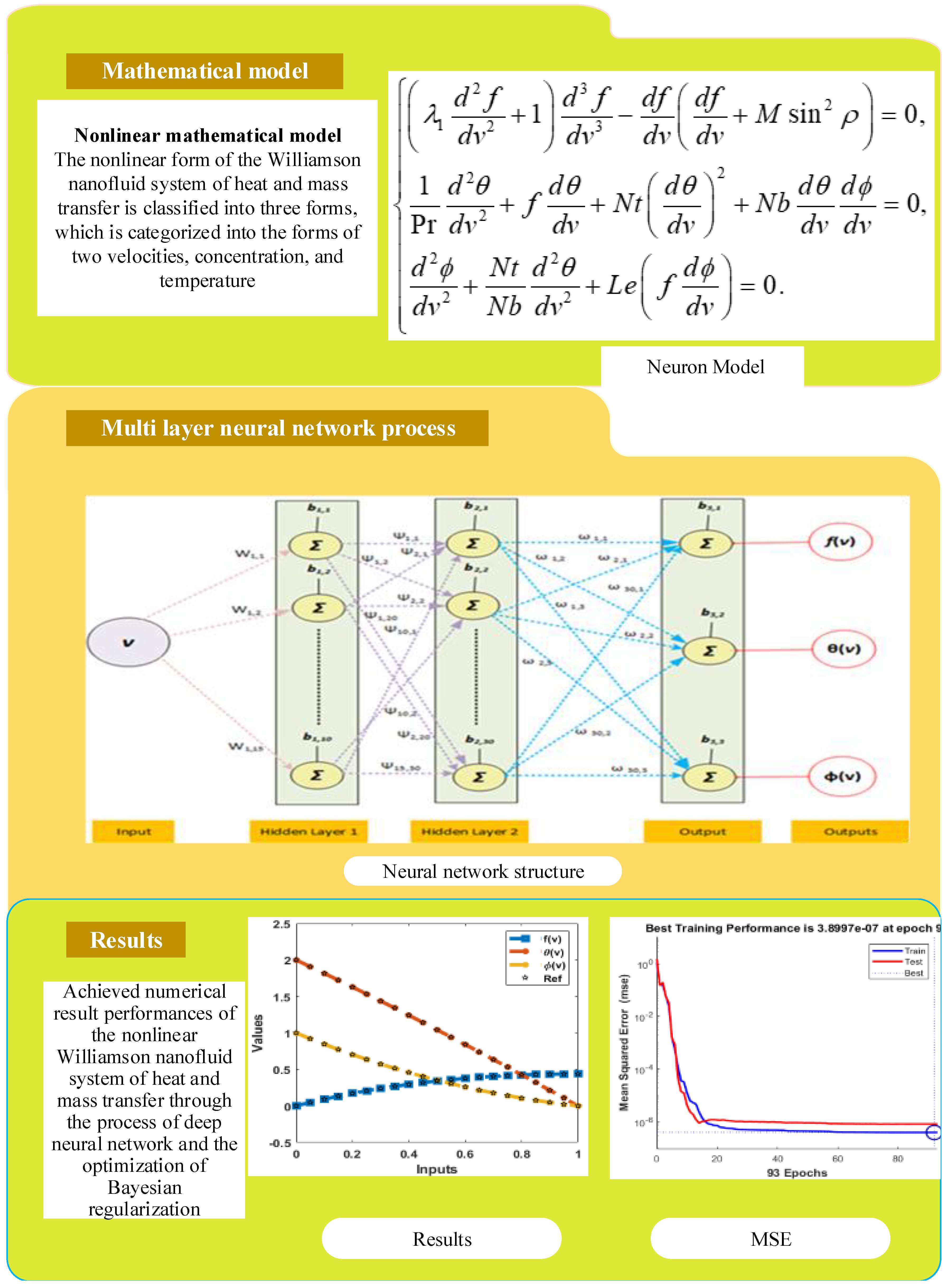
1. Introduction
- A learning deep neural network process is presented for the first time for the numerical solutions of the WNF system.
- A process of deep neural network using the amounts of fifteen and thirty neurons is presented for solving the model.
- The hyperbolic tangent sigmoid transfer function is used in the hidden layers.
- A Bayesian regularization for the optimization procedure is presented for solving the WNF system.
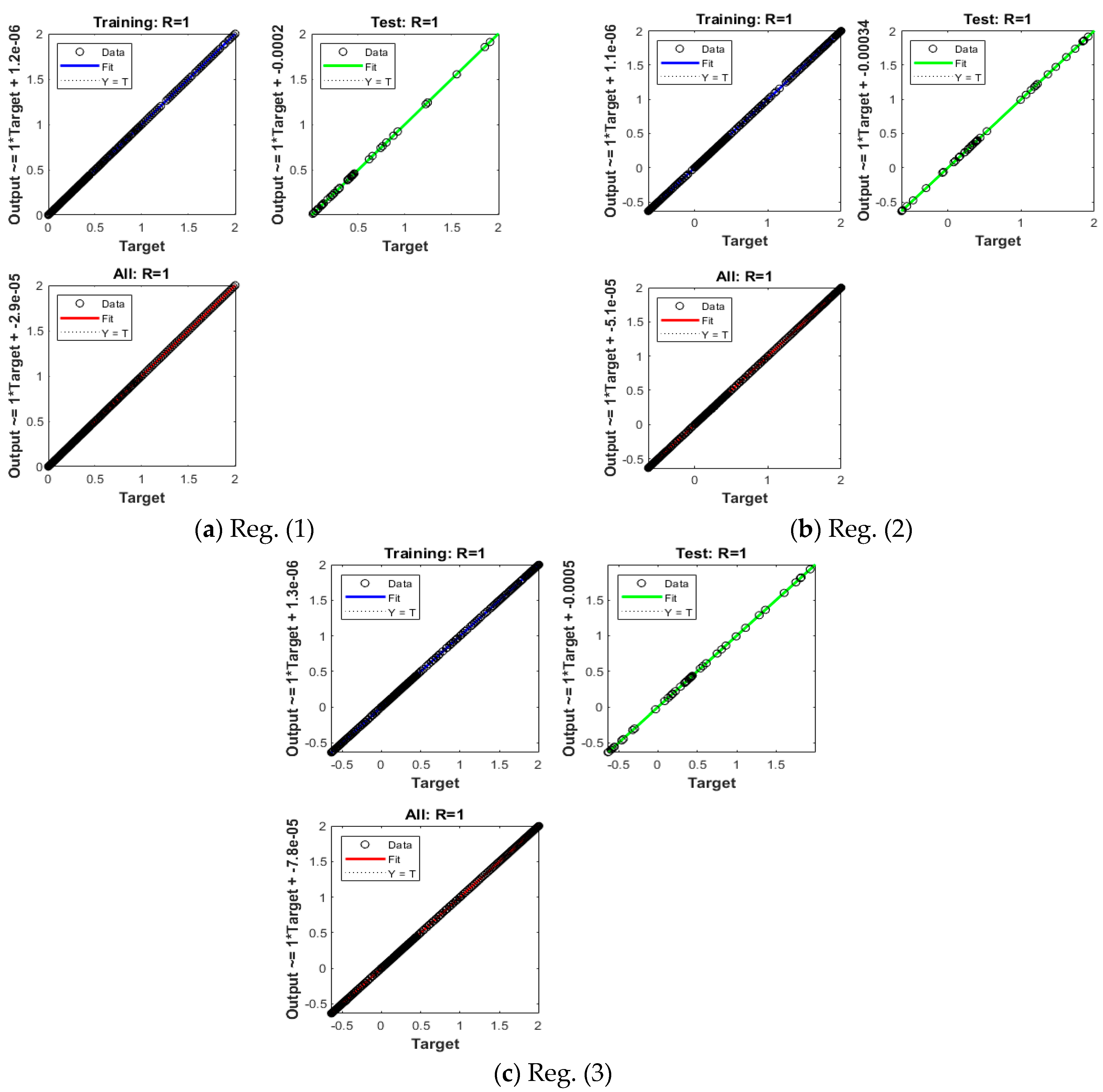
- A targeted dataset through the Adam scheme is achieved that is further accomplished based on training, testing, and verification with ratios of 0.15, 0.13, and 0.72.
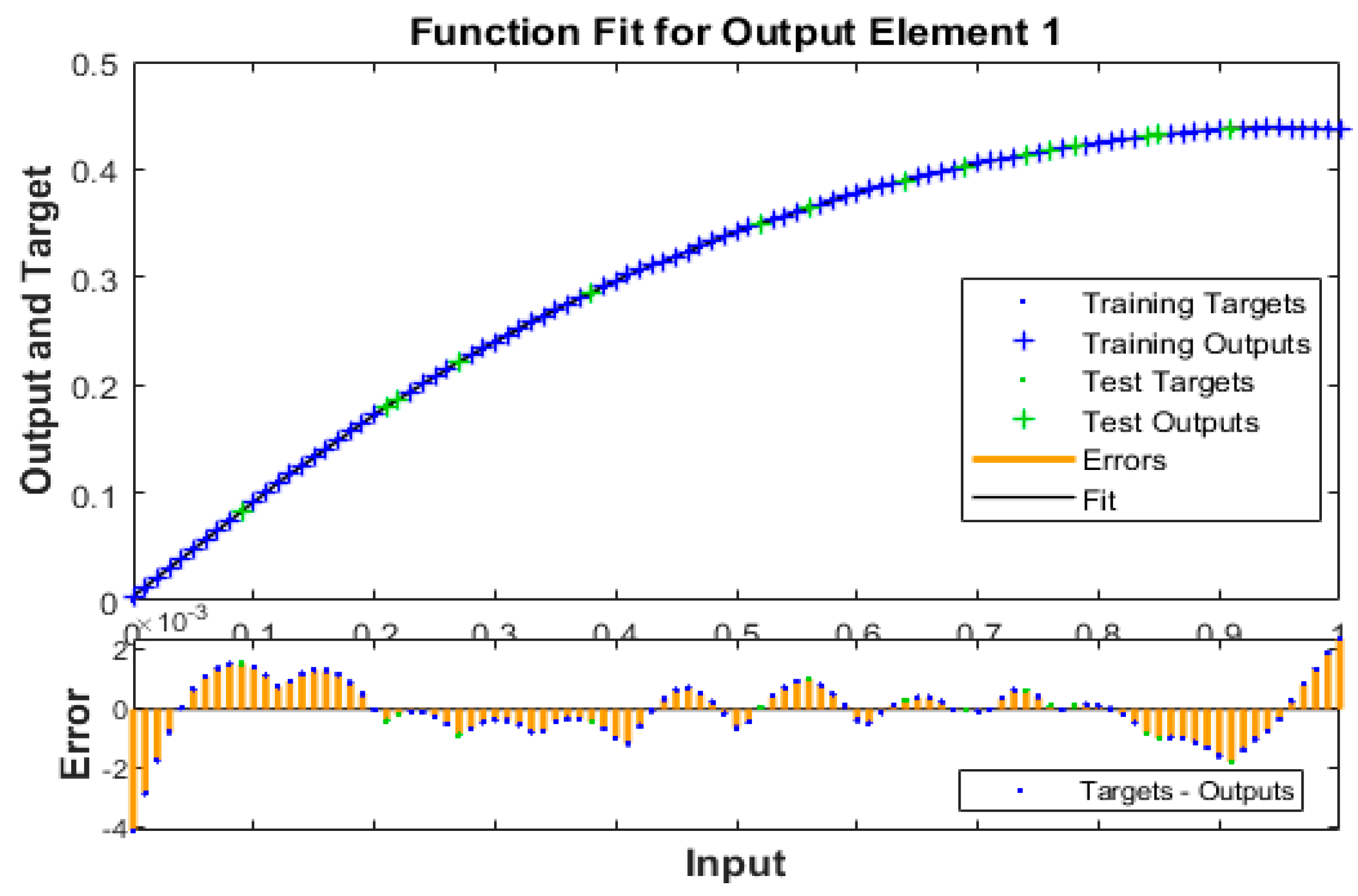
- The accuracy of the scheme is pragmatic through the comparison of the solutions, whereas the negligible absolute error (AE) enhances the correctness of the technique.
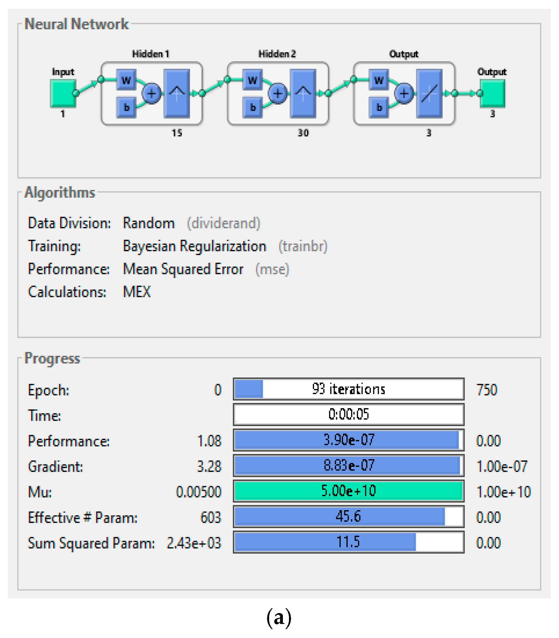
2. Methodology
2.1. Deep Neural Network Process
2.2. Bayesian Regularization (BR)
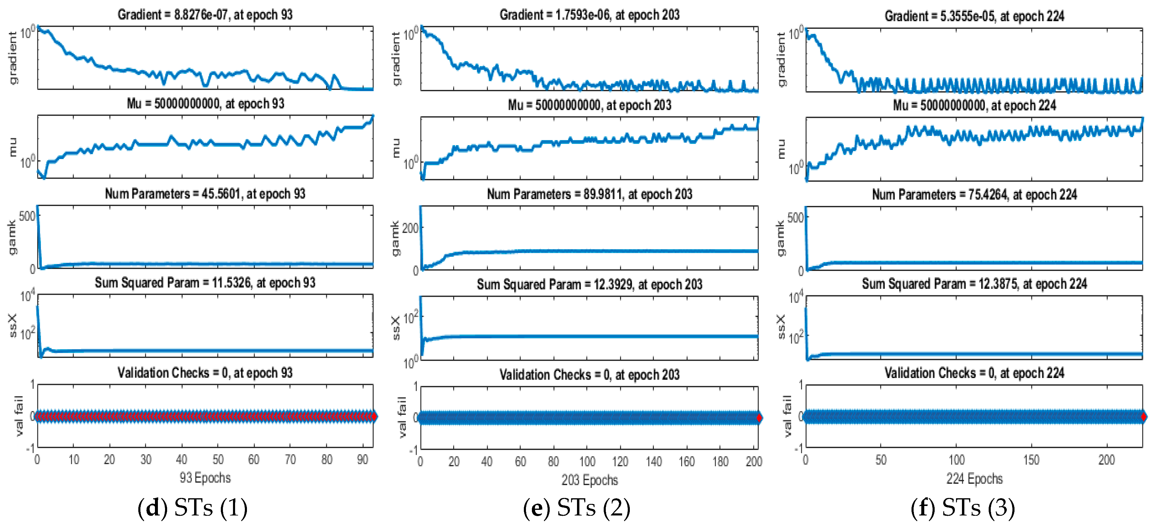
3. Simulations and Results
4. Concluding Remarks
- The optimization is performed through the Bayesian regularization, while the hyperbolic tangent sigmoid transfer function in the hidden layers is used.
- The numerical performances of the results have been proposed using the stochastic computing schemes along with the process of a deep neural network and Bayesian regularization.
- A targeted dataset ‘Adam’ scheme is designed, which is further accomplished based on the procedure of training, testing, and verification using the ratios of 0.15, 0.13, and 0.72.
- The correctness of the deep neural network along with BRA has been performed through the overlapping of the solutions and small absolute error.
- The capability of the procedure using the statistical observations is authenticated to reduce the mean square error for the nonlinear WNM.
Author Contributions
Funding
Data Availability Statement
Acknowledgments
Conflicts of Interest
References
- Bhatti, M.M.; Rashidi, M.M. Entropy generation with nonlinear thermal radiation in MHD boundary layer flow over a permeable shrinking/stretching sheet: Numerical solution. J. Nanofluids 2016, 5, 543–548. [Google Scholar] [CrossRef]
- Alharbi, K.A.M.; Yasmin, S.; Farooq, S.; Waqas, H.; Alwetaishi, M.; Khan, S.U.; Al-Turjman, F.; Elattar, S.; Khan, M.I.; Galal, A.M. Thermal outcomes of Williamson pseudo-plastic nanofluid with microorganisms due to the heated Riga surface with bio-fuel applications. Waves Random Complex Media 2022, 1–24. [Google Scholar] [CrossRef]
- Texter, J.; Qiu, Z.; Crombez, R.; Byrom, J.; Shen, W. Nanofluid acrylate composite resins—Initial preparation and characterization. Polym. Chem. 2011, 2, 1778–1788. [Google Scholar] [CrossRef]
- Krishnamurthy, M.; Prasannakumara, B.; Gireesha, B.; Gorla, R.S.R. Effect of chemical reaction on MHD boundary layer flow and melting heat transfer of Williamson nanofluid in porous medium. Eng. Sci. Technol. Int. J. 2016, 19, 53–61. [Google Scholar] [CrossRef]
- Hayat, T.; Anum Shafiq, A. Alsaedi, Hydromagnetic Boundary Layer Flow of Williamson Fluid in the Presence of Thermal Radiation and Ohmic Dissipation. Alex. Eng. J. 2016, 55, 2229–2240. [Google Scholar] [CrossRef]
- Bordag, M. Drude model and Lifshitz formula. Eur. Phys. J. C 2011, 71, 1788. [Google Scholar] [CrossRef]
- Bhatti, M.M.; Abbas, T.; Rashidi, M.M. Effects of thermal radiation and electromagnetohydrodynamics on viscous nanofluid through a Riga plate. Multidiscip. Model. Mater. Struct. 2016, 12, 605–618. [Google Scholar] [CrossRef]
- Goud, B.S.; Madhu, J.V.; Shekar, M.R. MHD Viscous Dissipative Fluid Flows In a Channel with a Stretching and Porous Plate with Radiation Effect. Int. J. Innov. Technol. Explor. Eng. 2019, 8, 1877–1882. [Google Scholar] [CrossRef]
- Kumar, P.P.; Goud, B.S.; Malga, B.S. Finite element study of Soret number effects on MHD flow of Jeffrey fluid through a vertical permeable moving plate. Partial. Differ. Equ. Appl. Math. 2020, 1, 100005. [Google Scholar] [CrossRef]
- Sreenadh, S.; Govardhan, P.; Kumar, Y.R. Effects of slip and heat transfer on the peristaltic pumping of a Williamson fluid in an inclined channel. Int. J. Appl. Sci. Eng. 2014, 12, 143–155. [Google Scholar]
- Rao, J.S.S.; Prasad, R.S.; Dharmavaram, A.D. Free Convective Fully Developed Flow of A Williamson Fluid in A Vertical Channel with An Effect of Inclined Magnetic Feild. J. Comput. Math. Sci. 2014, 5, 412–481. [Google Scholar]
- Ayub, A.; Sabir, Z.; Le, D.-N.; Aly, A.A. Nanoscale heat and mass transport of magnetized 3-D chemically radiative hybrid nanofluid with orthogonal/inclined magnetic field along rotating sheet. Case Stud. Therm. Eng. 2021, 26, 101193. [Google Scholar] [CrossRef]
- Ayub, A.; Wahab, H.A.; Shah, S.Z.; Shah, S.L.; Darvesh, A.; Haider, A.; Sabir, Z. Interpretation of infinite shear rate viscosity and a nonuniform heat sink/source on a 3D radiative cross nanofluid with buoyancy assisting/opposing flow. Heat Transf. 2021, 50, 4192–4232. [Google Scholar] [CrossRef]
- Nadeem, S.; Hussain, S.T. Flow and heat transfer analysis of Williamson nanofluid. Appl. Nanosci. 2013, 4, 1005–1012. [Google Scholar] [CrossRef]
- Venkataramanaiah, G.; Sreedharbabu, M.; Lavanya, M. Heat generation/absorption effects on magneto-williamson nanofluidflow with heat and mass fluxes. Int. J. Eng. Dev. Res. 2016, 4, 384–398. [Google Scholar]
- Hussanan, A.; Salleh, M.Z.; Khan, I. Microstructure and inertial characteristics of a magnetite ferrofluid over a stretching/shrinking sheet using effective thermal conductivity model. J. Mol. Liq. 2018, 255, 64–75. [Google Scholar] [CrossRef]
- Hussanan, A.; Qasim, M.; Chen, Z.-M. Heat transfer enhancement in sodium alginate based magnetic and non-magnetic nanoparticles mixture hybrid nanofluid. Phys. A Stat. Mech. Appl. 2020, 550, 123957. [Google Scholar] [CrossRef]
- Qureshi, M.Z.A.; Faisal, M.; Raza, Q.; Ali, B.; Botmart, T.; Shah, N.A.; Qureshi, M.Z.A.; Faisal, M.; Raza, Q.; Ali, B. Morphological nanolayer impact on hybrid nanofluids flow due to dispersion of polymer/CNT matrix nanocomposite material. AIMS Math. 2023, 8, 633–656. [Google Scholar] [CrossRef]
- Raza, Q.; Qureshi, M.Z.A.; Khan, B.A.; Hussein, A.K.; Ali, B.; Shah, N.A.; Chung, J.D. Insight into Dynamic of Mono and Hybrid Nanofluids Subject to Binary Chemical Reaction, Activation Energy, and Magnetic Field through the Porous Surfaces. Mathematics 2022, 10, 3013. [Google Scholar] [CrossRef]
- Khan, S.A.; Eze, C.; Lau, K.T.; Ali, B.; Ahmad, S.; Ni, S.; Zhao, J. Study on the novel suppression of heat transfer deterioration of supercritical water flowing in vertical tube through the suspension of alumina nanoparticles. Int. Commun. Heat Mass Transf. 2022, 132, 105893. [Google Scholar] [CrossRef]
- Lou, Q.; Ali, B.; Rehman, S.U.; Habib, D.; Abdal, S.; Shah, N.A.; Chung, J.D. Micropolar Dusty Fluid: Coriolis Force Effects on Dynamics of MHD Rotating Fluid When Lorentz Force Is Significant. Mathematics 2022, 10, 2630. [Google Scholar] [CrossRef]
- Ashraf, M.Z.; Rehman, S.U.; Farid, S.; Hussein, A.K.; Ali, B.; Shah, N.A.; Weera, W. Insight into Significance of Bioconvection on MHD Tangent Hyperbolic Nanofluid Flow of Irregular Thickness across a Slender Elastic Surface. Mathematics 2022, 10, 2592. [Google Scholar] [CrossRef]
- Ali, B.; Ali, M.; Saman, I.; Hussain, S.; Yahya, A.U.; Hussain, I. Tangent hyperbolic nanofluid: Significance of Lorentz and buoyancy forces on dynamics of bioconvection flow of rotating sphere via finite element simulation. Chin. J. Phys. 2022, 77, 658–671. [Google Scholar] [CrossRef]
- Ali, B.; Khan, S.A.; Hussein, A.K.; Thumma, T.; Hussain, S. Hybrid nanofluids: Significance of gravity modulation, heat source/ sink, and magnetohydrodynamic on dynamics of micropolar fluid over an inclined surface via finite element simulation. Appl. Math. Comput. 2021, 419, 126878. [Google Scholar] [CrossRef]
- Kho, Y.B.; Hussanan, A.; Mohamed, M.K.A.; Salleh, M.Z. Heat and mass transfer analysis on flow of Williamson nanofluid with thermal and velocity slips: Buongiorno model. Propuls. Power Res. 2019, 8, 243–252. [Google Scholar] [CrossRef]
- Shah, S.Z.H.; Wahab, H.A.; Ayub, A.; Sabir, Z.; Haider, A.; Shah, S.L. Higher order chemical process with heat transport of magnetized cross nanofluid over wedge geometry. Heat Transf. 2021, 50, 3196–3219. [Google Scholar] [CrossRef]
- Umar, M.; Sabir, Z.; Raja, M.A.Z.; Sánchez, Y.G. A stochastic numerical computing heuristic of SIR nonlinear model based on dengue fever. Results Phys. 2020, 19, 103585. [Google Scholar] [CrossRef]
- Sabir, Z. Neuron analysis through the swarming procedures for the singular two-point boundary value problems arising in the theory of thermal explosion. Eur. Phys. J. Plus 2022, 137, 638. [Google Scholar] [CrossRef]
- Sabir, Z. Stochastic numerical investigations for nonlinear three-species food chain system. Int. J. Biomath. 2022, 15, 2250005. [Google Scholar] [CrossRef]
- Umar, M.; Sabir, Z.; Raja, M.A.Z.; Baskonus, H.M.; Yao, S.-W.; Ilhan, E. A novel study of Morlet neural networks to solve the nonlinear HIV infection system of latently infected cells. Results Phys. 2021, 25, 104235. [Google Scholar] [CrossRef]
- Srinivasulu, T.; Goud, B.S. Effect of inclined magnetic field on flow, heat and mass transfer of Williamson nanofluid over a stretching sheet. Case Stud. Therm. Eng. 2021, 23, 100819. [Google Scholar] [CrossRef]
- Ilhan, E.; Kıymaz, I.O. A generalization of truncated M-fractional derivative and applications to fractional differential equations. Appl. Math. Nonlinear Sci. 2020, 5, 171–188. [Google Scholar] [CrossRef]
- Ammar, M.K.; Amin, M.R.; Hassan, M. Visibility intervals between two artificial satellites under the action of Earth oblateness. Appl. Math. Nonlinear Sci. 2018, 3, 353–374. [Google Scholar] [CrossRef]
- Baskonus, H.M.; Bulut, H.; Sulaiman, T.A. New Complex Hyperbolic Structures to the Lonngren-Wave Equation by Using Sine-Gordon Expansion Method. Appl. Math. Nonlinear Sci. 2019, 4, 129–138. [Google Scholar] [CrossRef]


| Parameters | Description |
|---|---|
| Nt | Thermophoresis parameter |
| M | Magnetic parameter |
| Bi | Biot number |
| ρ | Inclination angle |
| λ1 | Williamson parameter |
| Le | Lewis number |
| Pr | Prandtl number |
| Nb | Parameter of Brownian motion |
| Input |
| Case | MSE | Performance | Gradient | Epoch | Time | |
|---|---|---|---|---|---|---|
| Test | Train | |||||
| 1 | 8.1633 × 10−0.7 | 3.8997 × 10−0.7 | 3.90 × 10−0.7 | 8.83 × 10−0.7 | 93 | 5 s |
| 2 | 1.0091 × 10−0.6 | 3.8968 × 10−0.6 | 1.01 × 10−0.6 | 1.76 × 10−0.6 | 203 | 2 s |
| 3 | 1.1656 × 10−0.6 | 3.6107 × 10−0.6 | 1.17 × 10−0.6 | 5.36 × 10−0.5 | 224 | 12 s |
| v | 0 | 0.1 | 0.2 | 0.3 | 0.4 | 0.5 | 0.6 | 0.7 | 0.8 | 0.9 | 1 |
|---|---|---|---|---|---|---|---|---|---|---|---|
| 2 × 10⁻³ | 6 × 10⁻⁴ | 2 × 10⁻³ | 3 × 10⁻⁴ | 1 × 10⁻³ | 3 × 10⁻⁴ | 1 × 10⁻⁴ | 4 × 10⁻⁴ | 2 × 10⁻³ | 8 × 10⁻⁴ | 1 × 10⁻³ | |
| 1 × 10⁻³ | 7 × 10⁻⁴ | 1 × 10⁻³ | 1 × 10⁻³ | 3 × 10⁻⁴ | 2 × 10⁻⁴ | 9 × 10⁻⁴ | 5 × 10⁻⁵ | 3 × 10⁻⁴ | 1 × 10⁻⁴ | 1 × 10⁻³ | |
| 4 × 10⁻³ | 1 × 10⁻³ | 7 × 10⁻⁶ | 4 × 10⁻⁴ | 1 × 10⁻³ | 6 × 10⁻⁴ | 4 × 10⁻⁴ | 8 × 10⁻⁵ | 1 × 10⁻⁴ | 2 × 10⁻³ | 2 × 10⁻³ | |
| 2 × 10⁻⁴ | 3 × 10⁻⁴ | 4 × 10⁻⁴ | 8 × 10⁻⁵ | 4 × 10⁻⁴ | 7 × 10⁻⁵ | 2 × 10⁻⁵ | 2 × 10⁻⁴ | 7 × 10⁻⁴ | 3 × 10⁻⁴ | 4 × 10⁻⁴ | |
| 2 × 10⁻⁴ | 4 × 10⁻⁵ | 2 × 10⁻³ | 2 × 10⁻³ | 8 × 10⁻⁴ | 2 × 10⁻³ | 9 × 10⁻⁴ | 2 × 10⁻⁴ | 1 × 10⁻³ | 1 × 10⁻³ | 1 × 10⁻³ | |
| 1 × 10⁻³ | 3 × 10⁻⁴ | 8 × 10⁻⁴ | 2 × 10⁻⁴ | 4 × 10⁻⁴ | 8 × 10⁻⁴ | 3 × 10⁻⁴ | 4 × 10⁻⁴ | 6 × 10⁻⁴ | 1 × 10⁻³ | 2 × 10⁻³ | |
| 6 × 10⁻⁴ | 5 × 10⁻⁴ | 7 × 10⁻⁴ | 2 × 10⁻⁴ | 1 × 10⁻³ | 2 × 10⁻⁴ | 2 × 10⁻⁶ | 7 × 10⁻⁴ | 2 × 10⁻³ | 1 × 10⁻⁴ | 3 × 10⁻⁴ | |
| 2 × 10⁻³ | 8 × 10⁻⁴ | 5 × 10⁻³ | 5 × 10⁻³ | 2 × 10⁻³ | 1 × 10⁻³ | 2 × 10⁻⁴ | 1 × 10⁻³ | 5 × 10⁻⁴ | 7 × 10⁻⁴ | 2 × 10⁻⁴ | |
| 3 × 10⁻³ | 4 × 10⁻⁴ | 2 × 10⁻³ | 1 × 10⁻³ | 2 × 10⁻³ | 3 × 10⁻³ | 2 × 10⁻³ | 2 × 10⁻⁴ | 2 × 10⁻³ | 5 × 10⁻⁴ | 3 × 10⁻³ |
Disclaimer/Publisher’s Note: The statements, opinions and data contained in all publications are solely those of the individual author(s) and contributor(s) and not of MDPI and/or the editor(s). MDPI and/or the editor(s) disclaim responsibility for any injury to people or property resulting from any ideas, methods, instructions or products referred to in the content. |
© 2023 by the authors. Licensee MDPI, Basel, Switzerland. This article is an open access article distributed under the terms and conditions of the Creative Commons Attribution (CC BY) license (https://creativecommons.org/licenses/by/4.0/).
Share and Cite
Souayeh, B.; Sabir, Z. Designing Hyperbolic Tangent Sigmoid Function for Solving the Williamson Nanofluid Model. Fractal Fract. 2023, 7, 350. https://doi.org/10.3390/fractalfract7050350
Souayeh B, Sabir Z. Designing Hyperbolic Tangent Sigmoid Function for Solving the Williamson Nanofluid Model. Fractal and Fractional. 2023; 7(5):350. https://doi.org/10.3390/fractalfract7050350
Chicago/Turabian StyleSouayeh, Basma, and Zulqurnain Sabir. 2023. "Designing Hyperbolic Tangent Sigmoid Function for Solving the Williamson Nanofluid Model" Fractal and Fractional 7, no. 5: 350. https://doi.org/10.3390/fractalfract7050350
APA StyleSouayeh, B., & Sabir, Z. (2023). Designing Hyperbolic Tangent Sigmoid Function for Solving the Williamson Nanofluid Model. Fractal and Fractional, 7(5), 350. https://doi.org/10.3390/fractalfract7050350