Bifurcation and Stability of Two-Dimensional Activator–Inhibitor Model with Fractional-Order Derivative

Abstract

In organisms’ bodies, the activities of enzymes can be catalyzed or inhibited by some inorganic and organic compounds. The interaction between enzymes and these compounds is successfully described by mathematics. The main purpose of this article is to investigate the dynamics of the activator–inhibitor system (Gierer–Meinhardt system), which is utilized to describe the interactions of chemical and biological phenomena. The system is considered with a fractional-order derivative, which is converted to an ordinary derivative using the definition of the conformable fractional derivative. The obtained differential equations are solved using the separation of variables. The stability of the obtained positive equilibrium point of this system is analyzed and discussed. We find that this point can be locally asymptotically stable, a source, a saddle, or non-hyperbolic under certain conditions. Moreover, this article concentrates on exploring a Neimark–Sacker bifurcation and a period-doubling bifurcation. Then, we present some numerical computations to verify the obtained theoretical results. The findings of this work show that the governing system undergoes the Neimark–Sacker bifurcation and the period-doubling bifurcation under certain conditions. These types of bifurcation occur in small domains, as shown theoretically and numerically. Some 2D figures are illustrated to visualize the behavior of the solutions in some domains.

1. Introduction

Enzymes (or biocatalysts) are defined as proteinaceous molecules that can catalyze chemical reactions that occur within a cell. Enzymes act as catalysts for all types of chemical reactions occurring in human body, such as food digestion, blood coagulation, body growth, healing processes, reproduction mechanisms, and mechanisms of DNA replication, protein synthesis, etc. [1]. Normally, enzymes combine with a substrate to create an enzyme–substrate complex, which is then transformed into a final product. Then, the final product is disconnected from the original enzyme. The new free enzyme acts to transform another substrate into a final product [1]. Some inorganic and organic compounds known as “modifiers” change the catalytic activity of some enzymes. In other words, modifiers (or moderators) can increase or decrease the rate of an enzymatic reaction. Inhibition is a process that reduces or totally inhibits the enzyme’s catalytic activity, while activation is a process that increases the enzyme’s catalytic activity. In particular, compounds that reduce a chemical reaction (or an enzyme’s catalytic activity) are called inhibitors (negative modifiers), while compounds that help to speed up a chemical reaction and are not consumed during the chemical reaction are called activators (positive modifiers).

Nowadays, enzyme inhibitors are very beneficial due to their use in the remediation of many diseases. In many scientific specializations, such as biochemistry, biotechnology, and medicinal chemistry, enzyme inhibitors are considered an active area for most researchers. Some studies on enzyme inhibition have successfully contributed to providing useful information about ambiguous biological mechanisms, such as inflammatory reactions, blood coagulation, blood clot dissolution, etc. Moreover, enzyme inhibitors are classified into three main categories, namely, reversible enzyme inhibitors, irreversible enzyme inhibitors, and allosteric enzyme inhibitors. Reversible inhibitors (which can be divided into three main categories, namely, competitive, non-competitive, or uncompetitive) prevent the enzyme’s catalytic activity and noncovalently bind to the enzyme [2]. Hence, a free enzyme is separated from the molecule after a limited time. These types of inhibitors involve very weak interactions, such as hydrogen bonds and ionic bonds. However, irreversible inhibitors (which can be divided into two main categories, namely, suicide inhibitors and time-dependent inhibitors) covalently (strongly) bind to the enzyme and slowly dissociate from the enzyme [2]. Finally, allosteric inhibitors combine with the enzyme at an allosteric site and alter the structure of the active site of the enzyme [2].

The activator–inhibitor system (Gierer–Meinhardt system), which was developed in [3], is used to describe the interactions of chemical and biological phenomena. The dynamics of the activator–inhibitor system of an enzyme plays a crucial role in understanding the behavior of the catalytic activity of the enzyme inside a living organism. Therefore, some scientists have investigated the dynamical behaviors of this system using mathematics. For instance, Khan et al. [4] explored the stability of a unique equilibrium point, bifurcations, and chaos control for the discrete activator–inhibitor system. Pasemann et al. [5] developed a theory for diffusivity estimation for the activator–inhibitor model. Guo et al. [6] discussed the Turing patterns of the activator–inhibitor system on regular lattice networks. In addition, several complex networks were also examined in [6]. Song et al. [7] investigated the stability and the bifurcation of the activator–inhibitor system with a saturating term. Furthermore, Chen et al. [8] analyzed the stability of the equilibrium point of a general reaction–diffusion activator–inhibitor model. In [9], Chen investigated the long-time existence of solutions of the generalized activator–inhibitor model. Chen [9] also studied the blowup properties and boundedness of some special cases. The moving mesh method was used in [9] to approximate some numerical solutions for the generalized activator–inhibitor model. Ni et al. [10] explored the stability of stationary solutions for the activator–inhibitor system in higher-dimensional domains. More information about the qualitative behavior of biological systems can be found in refs. [11,12].

Fractional derivatives were discovered in $1695.$ Then, researchers developed some definitions for this type of derivative. For example, Laplace derived a beneficial concept for fractional derivatives of functions using integrals in 1812. In $1812,$ Lacroix developed the n-th fractional derivative of a given power function [13]. The first Liouville definition of the fractional derivative was presented by Liouville in 1832 [14]. Then, Riemann discovered his useful definition of fractional derivatives [15]. Furthermore, the Riemann–Liouville definition of a fractional derivative of a given function was successfully shown in the 19th century. Unfortunately, some of these definitions do not give accurate results for fractional derivatives. Therefore, we will use the most recent definition of the fractional derivative, which is the conformable fractional derivative [16].

Definition 1

([16]). Let $f:(0,\infty )\to \mathrm{R}$ be a function. Then, the conformable fractional derivative of order $0<\alpha \le 1$ of f at $t>0$ is defined by

$$T_h^{\alpha }f\left(t\right)=\underset{ϵ\to 0}{lim}\frac{f(t+ϵ{(t-h)}^{1-\alpha })-f\left(t\right)}{ϵ},0<\alpha <1,$$

(1)

where $T_h^{\alpha }$ is a fractional derivative of the conformable type, and $h>0$ is the discretization parameter. It was shown in [17] that the following fact is evidenced from Equation (1).

$$T_h^{\alpha }f\left(t\right)={(t-h)}^{1-\alpha }{f}^{\prime }\left(t\right).$$

(2)

This derivative has been applied by many researchers [18,19,20].

It is worth mentioning that the presented studies lack the usage of fractional derivatives. Motivated by the studies presented in the literature review, we investigate the existence of the equilibrium point and the stability conditions of the following activator–inhibitor system with fractional order:

$$\left\{\begin{array}{c}{T}^{\alpha }x\left(t\right)=p+\frac{x^2\left(t\right)}{y\left(t\right)}-x\left(t\right),\hfill \\ T^{\alpha }y\left(t\right)=x^2\left(t\right)-cy\left(t\right),\hfill \end{array}\right.$$

(3)

where $0<\alpha \le 1$ is the fractional-order parameter, and $t>0$. The variables $x\left(t\right)>0$ and $y\left(t\right)>0$ represent the concentrations of the activator and inhibitor, respectively. $p>0$ is the strength of self-activation of the activator with the gross activation of the inhibitor, and $c>0$ measures the strength of the production of the activator and that of itself. The conformable fractional derivative is used to obtain the corresponding ordinary derivatives. Then, we solve the obtained ordinary differential equations. The discretized version of the considered system will be analyzed in terms of bifurcations. Moreover, this study aims to discuss the existence of the Neimark–Sacker bifurcation and the period-doubling bifurcation of System (4) by selecting a suitable bifurcation parameter. Numerical computations are also shown to verify the obtained theoretical results. The dynamical properties of the proposed system will be clearly presented and explained via some figures.

This article is outlined as follows. Section 2 illustrates the discretization process of System (4). In Section 3, we analyze the stability of the obtained equilibrium point. Section 4 is devoted to discussing the bifurcation analysis of the considered system, while Section 5 presents the numerical computations and highlights the most important results. Finally, Section 6 concludes this article.

2. Discretization Process

In this section, we discretize System (3) by using the method of the piecewise constant argument [21]. Since $x\left(t\right)>0$ and $y\left(t\right)>0,$ System (3) can be written as

$$\left\{\begin{array}{c}\frac{T^{\alpha }x\left(t\right)}{x\left(t\right)}=\frac{p}{x\left(t\right)}+\frac{x\left(t\right)}{y\left(t\right)}-1,\hfill \\ \frac{T^{\alpha }y\left(t\right)}{y\left(t\right)}=\frac{x^2\left(t\right)}{y\left(t\right)}-c.\hfill \end{array}\right.$$

(4)

Using the method of the piecewise constant argument, System (4) becomes

$$\left\{\begin{array}{cc}\frac{T^{\alpha }x\left(t\right)}{x\left(t\right)}=\hfill & \frac{p}{x\left(\left[\frac{t}{h}\right]h\right)}+\frac{x\left(\left[\frac{t}{h}\right]h\right)}{y\left(\left[\frac{t}{h}\right]h\right)}-1,\hfill \\ \frac{T^{\alpha }y\left(t\right)}{y\left(t\right)}=\hfill & \frac{x^2\left(\left[\frac{t}{h}\right]h\right)}{y\left(\left[\frac{t}{h}\right]h\right)}-c,\hfill \end{array}\right.$$

(5)

with $x\left(t\right)>0$ and $y\left(t\right)>0$, where $\left[\frac{t}{h}\right]$ denotes the integer part of $t\in [0,\infty )$, $\alpha$ is a fractional parameter, and h is a discretization parameter. Applying Equations (1) and (2) to the first equation of System (5), we find

$${(t-nh)}^{1-\alpha }\frac{dx\left(t\right)}{x\left(t\right)dt}=\frac{p}{x\left(nh\right)}+\frac{x\left(nh\right)}{y\left(nh\right)}-1,$$

where $t\in [nh,(n+1\left)h\right)$. Integrating the previous equation on the interval $[nh,t)$ leads to

$$x\left(t\right)=x\left(nh\right)exp\left(\left(\frac{p}{x\left(nh\right)}+\frac{x\left(nh\right)}{y\left(nh\right)}-1\right)\frac{h^{\alpha }}{\alpha }\right).$$

This solution can be written in the form of difference equations by replacing $y\left(nh\right)$ and $x\left(nh\right)$ by $y_n$ and $x_n,$ respectively, as follows:

$$x_{n+1}=x_{n}exp\left(\left(\frac{p}{x_n}+\frac{x_n}{y_n}-1\right)\frac{h^{\alpha }}{\alpha }\right).$$

The second equation of System (5) is similarly solved to end up with

$$y_{n+1}=y_{n}exp\left(\left(\frac{x_n^2}{y_n}-c\right)\frac{h^{\alpha }}{\alpha }\right).$$

Therefore, we obtain the following two-dimensional difference equations:

$$\left\{\begin{array}{cc}{x}_{n+1}\hfill & {\displaystyle =x_n{e}^{\left(\frac{p}{x_n}+\frac{x_n}{y_n}-1\right)\frac{h^{\alpha }}{\alpha }},}\hfill \\ y_{n+1}\hfill & {\displaystyle =y_n{e}^{\left(\frac{x_n^2}{y_n}-c\right)\frac{h^{\alpha }}{\alpha }}.}\hfill \end{array}\right.$$

(6)

3. Stability Analysis

This section investigates the local asymptotic stability of System (6). The unique positive equilibrium point of System (6) is given by

$$P^{+}=\left(p+c,\frac{{(p+c)}^2}{c}\right).$$

The Jacobian matrix of System (6) at the point $P^{+}$ is given by

$$J\left(P^{+}\right)=\left(\begin{array}{cc}{\displaystyle 1+\frac{(c-p)h^{\alpha }}{\alpha (p+c)}}& {\displaystyle -\frac{c^2{h}^{\alpha }}{\alpha {(p+c)}^2}}\\ {\displaystyle \frac{2(p+c)h^{\alpha }}{\alpha }}& {\displaystyle 1-\frac{c{h}^{\alpha }}{\alpha }}\end{array}\right).$$

(7)

Then, the characteristic equation of the matrix $J\left(P^{+}\right)$ is shown as

$$\mathcal{F}\left(\mu \right)={\mu }^2-\mathcal{T}\mu +\mathcal{D}=0,$$

(8)

where

$$\begin{array}{c}{\displaystyle \mathcal{T}=2+\frac{h^{\alpha }}{\alpha }\left(\frac{c-p}{p+c}-c\right),}\hfill \\ {\displaystyle \mathcal{D}=1+\frac{h^{\alpha }}{\alpha }\left(\frac{c-p}{p+c}-c\right)+\frac{c{h}^{2\alpha }}{{\alpha }^2}.}\hfill \end{array}$$

Hence,

$$\mathcal{F}(-1)=4+\frac{2h^{\alpha }}{\alpha }\left(\frac{c-p}{p+c}-c\right)+\frac{c{h}^{2\alpha }}{{\alpha }^2},\mathcal{F}\left(0\right)=\mathcal{D},\mathcal{F}\left(1\right)=\frac{c{h}^{2\alpha }}{{\alpha }^2}>0.$$

Lemma 1

([22,23]). Let $\mathcal{F}\left(\mu \right)={\mu }^2-\mathcal{T}\mu +\mathcal{D}$, where $\mathcal{F}\left(1\right)>0$. Assume that μ and ${\mu }^{\prime }$ are the two roots of $\mathcal{F}\left(\mu \right)=0$. Then,

• If $\mathcal{F}(-1)>0$ and $\mathcal{F}\left(0\right)<1$, then $\mid \mu \mid <1$ and $\mid {\mu }^{\prime }\mid <1$, which implies that both eigenvalues have magnitudes less than 1.
• If $\mathcal{F}(-1)<0$, then $\mid \mu \mid <1$ and $\mid {\mu }^{\prime }\mid >1$ (or $\mid \mu \mid >1$ and $\mid {\mu }^{\prime }\mid <1$), which implies that one eigenvalue has a magnitude less than 1, while the other has a magnitude greater than 1.
• If $\mathcal{F}(-1)>0$ and $\mathcal{F}\left(0\right)>1$, then $\mid \mu \mid >1$ and $\mid {\mu }^{\prime }\mid >1$, which implies that both eigenvalues have magnitudes greater than 1.
• If $\left|T\right|<2$ and $\mathcal{F}\left(0\right)=1$, then μ and ${\mu }^{\prime }$ are complex numbers, and $\mid \mu \mid =\mid {\mu }^{\prime }\mid =1$, which implies that both eigenvalues are on the unit circle.
• $\mathcal{F}(-1)=0$ and $\mathcal{F}\left(0\right)\ne 0,1$ if and only if $\mu =-1$ and $\left|\mu \right|\ne 1.$

Given that $c>0$, it follows that $\mathcal{F}\left(1\right)>0$, and we can use Lemma (1) to state the following theorem.

Theorem 1.

For the fixed point $P^{+}$ of System (6), let

$$\begin{array}{c}{h}^{\mp }={\left(\frac{\alpha \left((p-c)+c(p+c)\mp \sqrt{{((p-c)+c(p+c))}^2-4c{(p+c)}^2}\right)}{c(p+c)}\right)}^{\frac{1}{\alpha }},h^{\prime }={\left(\alpha +\frac{\alpha \left(p-c\right)}{c(p+c)}\right)}^{\frac{1}{\alpha }}.\end{array}$$

Then, the following statements are true:

• If one set of the following conditions is true, then $P^{+}$ is locally asymptotically stable (sink):

  i-

  ${((p-c)+c(p+c))}^2-4c{(p+c)}^2<0$ and $0<h<h^{\prime }$.

  ii-

  ${((p-c)+c(p+c))}^2-4c{(p+c)}^2\ge 0$ and $0<h<h^{-}$.

• If one set of the following conditions is true, then $P^{+}$ is unstable (source):

  i-

  ${((p-c)+c(p+c))}^2-4c{(p+c)}^2<0$ and $h>h^{\prime }$.

  ii-

  ${((p-c)+c(p+c))}^2-4c{(p+c)}^2\ge 0$ and $h>h^{-}$.

• The fixed point $P^{+}$ is unstable (saddle) if

  $${((p-c)+c(p+c))}^2-4c{(p+c)}^2<0,and{h}^{-}<h<h^{+}.$$
• The point $P^{+}$ is non-hyperbolic and the roots of Equation (8) are $\mu =-1$ and $|{\mu }^{\prime }|\ne 1$ if

  $${((p-c)+c(p+c))}^2-4c{(p+c)}^2\ge 0,andh=h^{\mp }.$$
• The point $P^{+}$ is non-hyperbolic and the roots of Equation (8) are complex numbers with modulus one if

  $${((p-c)+c(p+c))}^2-4c{(p+c)}^2<0,andh=h^{\prime }.$$

4. Bifurcation Analysis

In this section, we discuss the existence of a Neimark–Sacker bifurcation and a period-doubling bifurcation [4,22,24,25,26,27,28,29,30] for System (6) by taking h as a bifurcation parameter.

4.1. Neimark–Sacker Bifurcation

This subsection is devoted to analyzing the Neimark–Sacker bifurcation for System (6) at the equilibrium point $P^{+}$ when the bifurcation parameter varies in a small neighborhood of the set

$${\mathcal{B}}_{NS}=\left\{\begin{array}{c}{\displaystyle (c,p,h,\alpha )\in {\mathrm{R}}^4\left|{((p-c)+c(p+c))}^2<4c{(p+c)}^2,\right.}\\ {\displaystyle h=h^{\prime }={\left(\alpha +\frac{\alpha (p-c)}{c(p+c)}\right)}^{\frac{1}{\alpha }},\alpha \in (0,1]}\end{array}\right\}.$$

Assume that $(c,p,h,\alpha )\in {\mathcal{B}}_{NS}$. Then, System (6) can be written as

$$\left\{{\displaystyle \begin{array}{cc}{x}_{n+1}\hfill & {\displaystyle =x_n{e}^{\left(\frac{p}{x_n}+\frac{x_n}{y_n}-1\right)\frac{{(h^{\prime }+\overline{h})}^{\alpha }}{\alpha }}=H_1(x_n,y_n,\overline{h}),}\hfill \\ y_{n+1}\hfill & {\displaystyle =y_n{e}^{\left(\frac{x_n^2}{y_n}-c\right)\frac{{(h^{\prime }+\overline{h})}^{\alpha }}{\alpha }}=H_2(x_n,y_n,\overline{h}),}\hfill \end{array}}\right.$$

(9)

where $\overline{h}$ is a small perturbation from $h^{\prime }$, and $\overline{h}\ll 1$. By using changes in the variables $z_n=x_n-(p+c)$ and $w_n=y_n-\left(\frac{{(p+c)}^2}{c}\right)$, we can shift the equilibrium point $P^{+}$ to the origin. Then, we expand $H_1$ and $H_2$ at the origin by using the Taylor series. Hence, System (9) becomes

$$\left\{{\displaystyle \begin{array}{cc}{z}_{n+1}\hfill & =a_{11}{z}_n+a_{12}{w}_n+a_{13}{z}_n^2+a_{14}{z}_n{w}_n+a_{15}{w}_n^2+\hfill \\ & a_{16}{z}_n^3+a_{17}{z}_n^2{w}_n+a_{18}{z}_n{w}_n^2+a_{19}{w}_n^3+{\mathcal{O}}_2\left(\right|z_n|,|w_n{\left|\right)}^4,\hfill \\ w_{n+1}\hfill & =a_{21}{z}_n+a_{22}{w}_n+a_{23}{z}_n^2+a_{24}{z}_n{w}_n+a_{25}{w}_n^2+\hfill \\ & a_{26}{z}_n^3+a_{27}{z}_n^2{w}_n+a_{28}{z}_n{w}_n^2+a_{29}{w}_n^3+{\mathcal{O}}_2\left(\right|z_n|,|w_n{\left|\right)}^4,\hfill \end{array}}\right.$$

(10)

where

$$\begin{array}{c}{a}_{11}=1+\frac{(c-p){(h^{\prime }+\overline{h})}^{\alpha }}{(p+c)\alpha },a_{12}=\frac{-c^2{(h^{\prime }+\overline{h})}^{\alpha }}{\alpha },a_{21}=\frac{2(p+c){(h^{\prime }+\overline{h})}^{\alpha }}{\alpha },a_{22}=1-\frac{c{(h^{\prime }+\overline{h})}^{\alpha }}{\alpha }.\end{array}$$

Note that the values of $a_{13}$, $a_{14},\cdots ,$$a_{19}$, $a_{23}$, $a_{24},\cdots ,a_{29}$ are given in Appendix A, with $h=(h^{\prime }+\overline{h})$. The characteristic equation of the Jacobian matrix of System (10), which is evaluated at the new shifted point, is given by

$${\mu }^2-\mathcal{T}\left(\overline{h}\right)\mu +\mathcal{D}\left(\overline{h}\right)=0,$$

(11)

where

$$\begin{array}{cc}{\displaystyle \mathcal{T}\left(\overline{h}\right)}\hfill & {\displaystyle =2+\frac{{(h^{\prime }+\overline{h})}^{\alpha }}{\alpha }\left(\frac{c-p}{p+c}-c\right),}\hfill \\ {\displaystyle \mathcal{D}\left(\overline{h}\right)}\hfill & {\displaystyle =1+\frac{{(h^{\prime }+\overline{h})}^{\alpha }}{\alpha }\left(\frac{c-p}{p+c}-c\right)+\frac{c{(h^{\prime }+\overline{h})}^{2\alpha }}{{\alpha }^2}.}\hfill \end{array}$$

Since $(c,p,h,\alpha )\in {\mathcal{B}}_{NS}$ and since Equation (11) has a pair of complex conjugate roots with a unit modulus, given by

$$\mu \left(\overline{h}\right),{\mu }^{\prime }\left(\overline{h}\right)=\frac{\mathcal{T}\left(\overline{h}\right)}{2}\pm \frac{i}{2}\sqrt{\left(4\mathcal{D}\left(\overline{h}\right)-\mathcal{T}{\left(\overline{h}\right)}^2\right)},$$

it follows that $|\mu \left(\overline{h}\right)|=|{\mu }^{\prime }\left(\overline{h}\right)|=\sqrt{\mathcal{D}\left(\overline{h}\right)}$, and

$${\left.\frac{d\left|\mu \right(\overline{h}\left)\right|}{d\overline{h}}\right|}_{\overline{h}=0}={\left.\frac{d|{\mu }^{\prime }\left(\overline{h}\right)|}{d\overline{h}}\right|}_{\overline{h}=0}=\frac{1}{2\sqrt{\mathcal{D}\left(0\right)}}{\left(\alpha +\frac{\alpha (p-c)}{c(p+c)}\right)}^{\frac{\alpha -1}{\alpha }}\left(c+\frac{p-c}{p+c}\right)>0.$$

The condition $\mathcal{T}\left(0\right)\ne 0,1$ leads to

$$h\ne \left(\frac{2(p+c)}{p-c+c(p+c)}\right),\left(\frac{(p+c)}{p-c+c(p+c)}\right),$$

(12)

which is equivalent to ${\left({\mu }^{\prime }\right)}^k,{\mu }^k\ne 1$ for $k=1,2,3,4$. In order to obtain the normal form of System (10) at $\overline{h}=0$, we use the following transformation:

$$\left(\begin{array}{c}{z}_n\\ w_n\end{array}\right)=\left(\begin{array}{cc}{a}_{12}& 0\\ \delta -a_{11}& -ϵ\end{array}\right)\left(\begin{array}{c}{\overline{x}}_n\\ {\overline{y}}_n\end{array}\right),$$

with $\delta =\Re \left(\mu \right)=\frac{\mathcal{T}\left(0\right)}{2}$ and $ϵ=\Im \left(\mu \right)=\frac{1}{2}\sqrt{(4\mathcal{D}\left(0\right)-\mathcal{T}{\left(0\right)}^2)}$. Using this transformation, System (10) reads as

$$\left\{\begin{array}{cc}{\overline{x}}_{n+1}=\hfill & \delta {\overline{x}}_n-ϵ{\overline{y}}_n+{\tilde{H}}_1(\overline{x},\overline{y},h^{\prime }),\hfill \\ {\overline{y}}_{n+1}=\hfill & ϵ{\overline{x}}_n+\delta {\overline{y}}_n+{\tilde{H}}_2(\overline{x},\overline{y},h^{\prime }),\hfill \end{array}\right.$$

(13)

where

$$\begin{array}{cc}{\displaystyle {\tilde{H}}_1({\overline{x}}_n,{\overline{y}}_n,h^{\prime })}\hfill & {\displaystyle =\frac{a_{13}}{a_{12}}{z}_n^2+\frac{a_{14}}{a_{12}}{z}_n{w}_n+\frac{a_{15}}{a_{12}}{w}_n^2+\frac{a_{16}}{a_{12}}{z}_n^3+\frac{a_{17}}{a_{12}}{z}_n^2{w}_n+\frac{a_{18}}{a_{12}}{z}_n{w}_n^2+}\hfill \\ & {\displaystyle \frac{a_{19}}{a_{12}}{w}_n^3+{\tilde{\mathcal{O}}}_1\left(\right|z_n|,|w_n{\left|\right)}^4,}\hfill \end{array}$$

$$\begin{array}{cc}{\displaystyle {\tilde{H}}_2({\overline{x}}_n,{\overline{y}}_n,h^{\prime })}\hfill & {\displaystyle =\left(\frac{a_{13}(\delta -a_{11})}{ϵa_{12}}-\frac{a_{23}}{ϵ}\right)z_n^2+\left(\frac{a_{14}(\delta -a_{11})}{ϵa_{12}}-\frac{a_{24}}{ϵ}\right)z_n{w}_n+}\hfill \\ & {\displaystyle \left(\frac{a_{15}(\delta -a_{11})}{ϵa_{12}}-\frac{a_{25}}{ϵ}\right)w_n^2+\left(\frac{a_{16}(\delta -a_{11})}{ϵa_{12}}-\frac{a_{26}}{ϵ}\right)z_n^3+}\hfill \\ & {\displaystyle \left(\frac{a_{17}(\delta -a_{11})}{ϵa_{12}}-\frac{a_{27}}{ϵ}\right)z_n^2{w}_n+\left(\frac{a_{18}(\delta -a_{11})}{ϵa_{12}}-\frac{a_{28}}{ϵ}\right)z_n{w}_n^2+}\hfill \\ & {\displaystyle \left(\frac{a_{19}(\delta -a_{11})}{ϵa_{12}}-\frac{a_{29}}{ϵ}\right)w_n^3+{\tilde{\mathcal{O}}}_2\left(\right|z_n|,|w_n{\left|\right)}^4,}\hfill \end{array}$$

and

$$z_n=a_{12}{\overline{x}}_n,w_n=(\delta -a_{11}){\overline{x}}_n-ϵ{\overline{y}}_n.$$

Finally, in order to determine the conditions under which the Neimark–Sacker bifurcation exists, we consider the following nonzero expression:

$$\mathcal{L}=\Re \left({\mu }^{\prime }{\mathrm{t}}_{21}\right)-\Re \left(\frac{(1-2\mu ){\left({\mu }^{\prime }\right)}^2}{1-\mu }{\mathrm{t}}_{20}{\mathrm{t}}_{11}\right)-\frac{1}{2}|{\mathrm{t}}_{11}{|}^2-{\left|{\mathrm{t}}_{02}\right|}^2,$$

(14)

where

$$\begin{array}{cc}\hfill {\mathrm{t}}_{20}& ={\left.\frac{1}{8}\left[\frac{{\partial }^2{\tilde{H}}_1}{\partial {\overline{x}}^2}-\frac{{\partial }^2{\tilde{H}}_1}{\partial {\overline{y}}^2}+2\frac{{\partial }^2{\tilde{H}}_2}{\partial \overline{x}\partial \overline{y}}+i\left(\frac{{\partial }^2{\tilde{H}}_2}{\partial {\overline{x}}^2}-\frac{{\partial }^2{\tilde{H}}_2}{\partial {\overline{y}}^2}-2\frac{{\partial }^2{\tilde{H}}_1}{\partial \overline{x}\partial \overline{y}}\right)\right]\right|}_{\overline{h}=0},\hfill \\ \hfill {\mathrm{t}}_{11}& ={\left.\frac{1}{4}\left[\frac{{\partial }^2{\tilde{H}}_1}{\partial {\overline{x}}^2}+\frac{{\partial }^2{\tilde{H}}_1}{\partial {\overline{y}}^2}+i\left(\frac{{\partial }^2{\tilde{H}}_2}{\partial {\overline{x}}^2}+\frac{{\partial }^2{\tilde{H}}_2}{\partial {\overline{y}}^2}\right)\right]\right|}_{\overline{h}=0},\hfill \\ \hfill {\mathrm{t}}_{02}& ={\left.\frac{1}{8}\left[\frac{{\partial }^2{\tilde{H}}_1}{\partial {\overline{x}}^2}-\frac{{\partial }^2{\tilde{H}}_1}{\partial {\overline{y}}^2}-2\frac{{\partial }^2{\tilde{H}}_2}{\partial \overline{x}\partial \overline{y}}+i\left(\frac{{\partial }^2{\tilde{H}}_2}{\partial {\overline{x}}^2}-\frac{{\partial }^2{\tilde{H}}_2}{\partial {\overline{y}}^2}+2\frac{{\partial }^2{\tilde{H}}_1}{\partial \overline{x}\partial \overline{y}}\right)\right]\right|}_{\overline{h}=0},\hfill \\ \hfill {\mathrm{t}}_{21}& ={\left.\frac{1}{16}\left[\frac{{\partial }^3{\tilde{H}}_1}{\partial {\overline{x}}^3}+\frac{{\partial }^3{\tilde{H}}_1}{\partial \overline{x}\partial {\overline{y}}^2}+\frac{{\partial }^3{\tilde{H}}_2}{\partial {\overline{x}}^2\partial \overline{y}}+\frac{{\partial }^3{\tilde{H}}_2}{\partial {\overline{y}}^3}+i\left(\frac{{\partial }^3{\tilde{H}}_2}{\partial {\overline{x}}^3}+\frac{{\partial }^3{\tilde{H}}_2}{\partial \overline{x}\partial {\overline{y}}^2}-\frac{{\partial }^3{\tilde{H}}_1}{\partial {\overline{x}}^2\partial \overline{y}}-\frac{{\partial }^3{\tilde{H}}_1}{\partial {\overline{y}}^3}\right)\right]\right|}_{\overline{h}=0}.\hfill \end{array}$$

Theorem 2.

Assume that Condition (12) is satisfied, and let $(c,p,h,\alpha )\in {\mathcal{B}}_{NS}$ with $\mathcal{L}\ne 0$. Then, System (10) undergoes a Neimark–Sacker bifurcation at the equilibrium point $P^{+}=\left(p+c,\frac{{(p+c)}^2}{c}\right)$ when the bifurcation parameter h varies in a small neighborhood of

$$h^{\prime }={\left(\alpha +\frac{\alpha (p-c)}{c(p+c)}\right)}^{\frac{1}{\alpha }}.$$

Moreover, if $\mathcal{L}<0$ ($\mathcal{L}>0$), then an attracting (respectively, repelling) closed invariant curve bifurcates from the equilibrium point $P^{+}=\left(p+c,\frac{{(p+c)}^2}{c}\right)$ for $h>h^{\prime }$ (respectively, $h<h^{\prime }$).

4.2. Period-Doubling Bifurcation

In this subsection, the period-doubling bifurcation [28] is studied at the equilibrium point $P^{+}$ when the bifurcation parameter varies in a small neighborhood of the set

$${\mathcal{B}}_{PB}=\left\{\begin{array}{c}(c,p,h,\alpha )\in {\mathrm{R}}^4\left|\alpha \in (0,1],{((p-c)+c(p+c))}^2\ge 4c{(p+c)}^2,h\ne {\left(\alpha +\frac{\alpha (p-c)}{c(p+c)}\right)}^{\frac{1}{\alpha }}\right.\hfill \\ {\displaystyle h=h^{-}={\left(\frac{\alpha \left((p-c)+c(p+c)-\sqrt{{((p-c)+c(p+c))}^2-4c{(p+c)}^2}\right)}{c(p+c)}\right)}^{\frac{1}{\alpha }}}\hfill \end{array}\right\}.$$

It is worth noting that one can similarly use the bifurcation parameter $h=h^{+}$ when it varies in a small neighborhood of the set ${\mathcal{B}}_{PB}.$ Suppose that $(c,p,h,\alpha )\in {\mathcal{B}}_{PD}$. Then, System (6) can be written as

$$\left\{{\displaystyle \begin{array}{cc}{x}_{n+1}\hfill & {\displaystyle =x_n{e}^{\left(\frac{p}{x_n}+\frac{x_n}{y_n}-1\right)\frac{{(h^{-}+\overline{h})}^{\alpha }}{\alpha }}=H_1(x_n,y_n,\overline{h}),}\hfill \\ y_{n+1}\hfill & {\displaystyle =y_n{e}^{\left(\frac{x_n^2}{y_n}-c\right)\frac{{(h^{-}+\overline{h})}^{\alpha }}{\alpha }}=H_2(x_n,y_n,\overline{h}),}\hfill \end{array}}\right.$$

(15)

where $\overline{h}$ is a small perturbation from $h^{-}$, and $\overline{h}\ll 1$. By utilizing changes in the variables $z_n=x_n-(p+c)$ and $w_n=y_n-\left(\frac{{(p+c)}^2}{c}\right)$, we can translate the equilibrium point $P^{+}$ to the origin. Then, we expand $H_1$ and $H_2$ at the origin using the Taylor series. Achieving this, System (15) becomes

$$\left\{{\displaystyle \begin{array}{cc}{z}_{n+1}=\hfill & a_{11}{z}_n+a_{12}{w}_n+a_{13}{z}_n^2+a_{14}{z}_n{w}_n+a_{15}{w}_n^2+b_{11}{z}_n\overline{h}+b_{12}{w}_n\overline{h}+a_{16}{z}_n^3+\hfill \\ \hfill & b_{13}{\overline{h}}^2+b_{14}{z}_n^2\overline{h}+b_{15}{w}_n^2\overline{h}+a_{17}{z}_n^2{w}_n+a_{18}{z}_n{w}_n^2+b_{16}{z}_n{w}_n\overline{h}+b_{17}{\overline{h}}^3+\hfill \\ \hfill & b_{18}{z}_n{\overline{h}}^2+b_{19}{w}_n{\overline{h}}^2+a_{19}{w}_n^3+{\mathcal{O}}_2\left(\right|z_n|,|w_n|,|\overline{h}{\left|\right)}^4,\hfill \\ w_{n+1}=\hfill & a_{21}{z}_n+a_{22}{w}_n+a_{23}{z}_n^2+a_{24}{z}_n{w}_n+a_{25}{w}_n^2+b_{21}{z}_n\overline{h}+b_{22}{w}_n\overline{h}+a_{26}{z}_n^3+\hfill \\ \hfill & b_{23}{\overline{h}}^2+b_{24}{z}_n^2\overline{h}+b_{25}{w}_n^2\overline{h}++a_{27}{z}_n^2{w}_n+a_{28}{z}_n{w}_n^2+b_{26}{z}_n{w}_n\overline{h}+b_{27}{\overline{h}}^3+\hfill \\ \hfill & b_{28}{z}_n{\overline{h}}^2+b_{29}{w}_n{\overline{h}}^2+a_{29}{w}_n^3+{\mathcal{O}}_2\left(\right|z_n|,|w_n|,|\overline{h}{\left|\right)}^4,\hfill \end{array}}\right.$$

(16)

where

$$\begin{array}{c}{a}_{11}=1+\frac{(c-p){(h^{-}+\overline{h})}^{\alpha }}{(p+c)\alpha },a_{12}=\frac{-c^2{(h^{-}+\overline{h})}^{\alpha }}{\alpha },a_{21}=\frac{2(p+c){(h^{-}+\overline{h})}^{\alpha }}{\alpha },a_{22}=1-\frac{c{(h^{-}+\overline{h})}^{\alpha }}{\alpha }.\end{array}$$

It is worth noting that the values of $a_{13}$, $a_{14},\cdots ,$$a_{19}$, $a_{23}$, $a_{24},\cdots ,a_{29}$, $b_{11}$, $b_{12},\cdots ,b_{19}$, $b_{21}$, $b_{22},\cdots ,b_{29}$ are given in Appendix A with $h=(h^{-}+\overline{h})$. Now, we determine the normal form of System (16) at $\overline{h}$ by using the transformation:

$$\left(\begin{array}{c}{z}_n\\ w_n\end{array}\right)=\left(\begin{array}{cc}{a}_{12}& a_{12}\\ -1-a_{11}& {\mu }^{\prime }-a_{11}\end{array}\right)\left(\begin{array}{c}{\overline{x}}_n\\ {\overline{y}}_n\end{array}\right).$$

Hence, System (16) becomes

$$\left\{\begin{array}{cc}{\overline{x}}_{n+1}=\hfill & \delta {\overline{x}}_n-ϵ{\overline{y}}_n+{\tilde{H}}_1(\overline{x},\overline{y},h^{-}),\hfill \\ {\overline{y}}_{n+1}=\hfill & ϵ{\overline{x}}_n+\delta {\overline{y}}_n+{\tilde{H}}_2(\overline{x},\overline{y},h^{-}).\hfill \end{array}\right.$$

(17)

where

$$\begin{array}{c}{\tilde{H}}_1(\overline{x},\overline{y},\overline{h})=\left(\frac{a_{13}({\mu }^{\prime }-a_{11})-a_{12}{a}_{23}}{a_{12}(1+{\mu }^{\prime })}\right)z_n^2+\left(\frac{a_{14}({\mu }^{\prime }-a_{11})-a_{12}{a}_{24}}{a_{12}(1+{\mu }^{\prime })}\right)z_n{w}_n+\left(\frac{a-15({\mu }^{\prime }-a_{11})-a_{12}{a}_{25}}{a_{12}(1+{\mu }^{\prime })}\right)w_n^2\hfill \\ +\left(\frac{b_{11}({\mu }^{\prime }-a_{11})-a_{12}{b}_{21}}{a_{12}(1+{\mu }^{\prime })}\right)z_n\overline{h}+\left(\frac{b_{12}({\mu }^{\prime }-a_{11})-a_{12}{b}_{22}}{a_{12}(1+\mu )}\right)w_n\overline{h}+\left(\frac{a_{16}({\mu }^{\prime }-a_{11})-a_{12}{a}_{26}}{a_{12}(1+{\mu }^{\prime })}\right)z_n^3\hfill \\ +\left(\frac{b_{13}({\mu }^{\prime }-a_{11})-a_{12}{b}_{23}}{a_{12}(1+{\mu }^{\prime })}\right){\overline{h}}^2+\left(\frac{b_{14}({\mu }^{\prime }-a_{11})-a_{12}{b}_{24}}{a_{12}(1+{\mu }^{\prime })}\right)z_n^2\overline{h}+\left(\frac{b_{15}({\mu }^{\prime }-a_{11})-a_{12}{b}_{25}}{a_{12}(1+{\mu }^{\prime })}\right)w_n^2\overline{h}\hfill \\ +\left(\frac{a_{17}({\mu }^{\prime }-a_{11})-a_{12}{a}_{27}}{a_{12}(1+{\mu }^{\prime })}\right)z_n^2{w}_n+\left(\frac{a_{18}({\mu }^{\prime }-a_{11})-a_{12}{a}_{28}}{a_{12}(1+{\mu }^{\prime })}\right)z_n{w}_n^2+\left(\frac{b_{16}({\mu }^{\prime }-a_{11})-a_{12}{b}_{26}}{a_{12}(1+{\mu }^{\prime })}\right)z_n{w}_n\overline{h}\hfill \\ +\left(\frac{b_{17}({\mu }^{\prime }-a_{11})-a_{12}{b}_{27}}{a_{12}(1+{\mu }^{\prime })}\right){\overline{h}}^3+\left(\frac{b_{18}({\mu }^{\prime }-a_{11})-a_{12}{b}_{28}}{a_{12}(1+{\mu }^{\prime })}\right)z_n{\overline{h}}^2+\left(\frac{b_{19}({\mu }^{\prime }-a_{11})-a_{12}{b}_{29}}{a_{12}(1+{\mu }^{\prime })}\right)w_n{\overline{h}}^2\hfill \\ +\left(\frac{a_{19}({\mu }^{\prime }-a_{11})-a_{12}{a}_{29}}{a_{12}(1+{\mu }^{\prime })}\right)w_n^3+{\mathcal{O}}_1\left(\right|z_n|,|w_n|,|\overline{h}{\left|\right)}^4,\hfill \end{array}$$

and

$$\begin{array}{c}{\tilde{H}}_2(\overline{x},\overline{y},\overline{h})=\left(\frac{a_{13}(1-a_{11})+a_{12}{a}_{23}}{a_{12}(1+{\mu }^{\prime })}\right)z_n^2+\left(\frac{a_{14}(1-a_{11})+a_{12}{a}_{24}}{a_{12}(1+{\mu }^{\prime })}\right)z_n{w}_n+\left(\frac{a-15(1-a_{11})+a_{12}{a}_{25}}{a_{12}(1+{\mu }^{\prime })}\right)w_n^2\hfill \\ +\left(\frac{b_{11}(1-a_{11})+a_{12}{b}_{21}}{a_{12}(1+{\mu }^{\prime })}\right)z_n\overline{h}+\left(\frac{b_{12}(1-a_{11})+a_{12}{b}_{22}}{a_{12}(1+\mu )}\right)w_n\overline{h}+\left(\frac{a_{16}(1-a_{11})+a_{12}{a}_{26}}{a_{12}(1+{\mu }^{\prime })}\right)z_n^3\hfill \\ +\left(\frac{b_{13}(1-a_{11})+a_{12}{b}_{23}}{a_{12}(1+{\mu }^{\prime })}\right){\overline{h}}^2+\left(\frac{b_{14}(1-a_{11})+a_{12}{b}_{24}}{a_{12}(1+{\mu }^{\prime })}\right)z_n^2\overline{h}+\left(\frac{b_{15}(1-a_{11})+a_{12}{b}_{25}}{a_{12}(1+{\mu }^{\prime })}\right)w_n^2\overline{h}\hfill \\ +\left(\frac{a_{17}(1-a_{11})+a_{12}{a}_{27}}{a_{12}(1+{\mu }^{\prime })}\right)z_n^2{w}_n+\left(\frac{a_{18}(1-a_{11})+a_{12}{a}_{28}}{a_{12}(1+{\mu }^{\prime })}\right)z_n{w}_n^2\left(\frac{b_{16}(1-a_{11})+a_{12}{b}_{26}}{a_{12}(1+{\mu }^{\prime })}\right)z_n{w}_n\overline{h}\hfill \\ \left(\frac{b_{17}(1-a_{11})+a_{12}{b}_{27}}{a_{12}(1+{\mu }^{\prime })}\right){\overline{h}}^3\left(\frac{b_{18}(1-a_{11})+a_{12}{b}_{28}}{a_{12}(1+{\mu }^{\prime })}\right)z_n{\overline{h}}^2\left(\frac{b_{19}(1-a_{11})+a_{12}{b}_{29}}{a_{12}(1+{\mu }^{\prime })}\right)w_n{\overline{h}}^2\hfill \\ +\left(\frac{a_{19}(1-a_{11})+a_{12}{a}_{29}}{a_{12}(1+{\mu }^{\prime })}\right)w_n^3+{\mathcal{O}}_2\left(\right|z_n|,|w_n|,|\overline{h}{\left|\right)}^4,\hfill \end{array}$$

with

$$z_n=a_{12}(\overline{x}+\overline{y})\mathrm{and}{w}_n=-(1+a_{11})\overline{x}+({\mu }^{\prime }-a_{11})\overline{y}.$$

Thus, the approximation of the center manifold ${\mathrm{M}}^c(0,0,0)$ of System (17) within the neighborhood of $\overline{h}=0$ is evaluated at the origin to obtain

$${\mathrm{M}}^c(0,0,0)=\left\{(\overline{x},\overline{y})\in {\mathrm{R}}^2:\overline{y}=m_1{\overline{x}}^2+m_2\overline{x}\overline{h}+m_3{\overline{h}}^2+\mathcal{O}{(\overline{x},\overline{h})}^3\right\},$$

where

$$m_1=\left(\frac{(a_{13}{a}_{12}-a_{12}{a}_{24})(1+a_{11})-a_{12}^2{a}_{23}-(a_{14}-a_{26}){(1+a_{11})}^2}{(1-{\left({\mu }^{\prime }\right)}^2)}+\frac{a_{16}{(1+a_{11})}^3}{a_{12}(1-{\left({\mu }^{\prime }\right)}^2)}\right),$$

$$m_2=\left(\frac{(b_{11}-b_{22})(1+a_{11})-a_{12}{b}_{12}}{(1-{\left({\mu }^{\prime }\right)}^2)}+\frac{b_{12}{(1+a_{11})}^2}{a_{12}(1-{\left({\mu }^{\prime }\right)}^2)}\right),$$

and

$$m_3=\frac{b_{13}(1-a_{11})-a_{12}{b}_{23}}{a_{12}(1-{\left({\mu }^{\prime }\right)}^2)}.$$

Thus, System (17) is restricted to the center manifold ${\mathrm{M}}^c(0,0,0)$ as follows:

$$\varphi :\overline{x}\to -\overline{x}+s_1{\overline{x}}^2+s_2\overline{x}\overline{h}+s_3{\overline{x}}^2\overline{h}+s_4\overline{x}{\overline{h}}^2+s_5{\overline{x}}^3+\mathcal{O}{(\overline{x},\overline{h})}^4,$$

where

$$s_1=\frac{({\mu }^{\prime }-a_{11})(a_{13}{a}_{12}-a_{14}(1+a_{11}))+a_{12}(a_{24}(1+a_{11})-a_{23}{a}_{12})}{(1+{\mu }^{\prime })}$$

$$+\frac{{(1+a_{11})}^2(a_{15}({\mu }^{\prime }-a_{11})-a_{24}{a}_{12})}{a_{12}(1+{\mu }^{\prime })},$$

$$s_2=\frac{({\mu }^{\prime }+a_{11})(a_{12}{b}_{11}-b_{12}(1+a_{11}))+a_{12}(b_{22}(1+a_{11})-b_{21}{a}_{12})}{a_{12}(1+{\mu }^{\prime })},$$

$$s_3=\frac{({\mu }^{\prime }+a_{11})(a_{12}{b}_{14}-b_{16}(1+a_{11}))-a_{12}(a_{12}{b}_{24}+(1+a_{11})b_{26})-b_{25}{(1+a_{11})}^2}{\left(1{\mu }^{\prime }\right)}$$

$$+\frac{b_{15}({\mu }^{\prime }+a_{11}){(1+a_{11})}^2}{a_{12}(1+{\mu }^{\prime })},$$

$$s_4=\frac{b_{18}({\mu }^{\prime }+a_{11})-b_{28}{a}_{12}+b_{29}(1+a_{11})}{(1+{\mu }^{\prime })}-\frac{b_{19}{({\mu }^{\prime }+a_{11})}^2}{a_{12}(1+{\mu }^{\prime })},$$

$$s_5=\frac{({\mu }^{\prime }-a_{11})(a_{14}{a}_{12}^2+a_{16}{(1+a_{11})}^2-a_{15}{a}_{12}(1+a_{11}))-a_{24}{a}_{12}^3+a_{25}{a}_{12}^2(1+g_{11})}{(1+{\mu }^{\prime })}$$

$$+\frac{a_{27}{a}_{12}{(1+a_{11})}^3-a_{26}{a}_{12}^2{(1+a_{11})}^2-a_{17}({\mu }^{\prime }-a_{11}){(1+a_{11})}^3}{a_{12}(1+{\mu }^{\prime })}.$$

Suppose that

$${\mathcal{X}}_1={\left.\left(\frac{{\partial }^2\varphi }{\partial \overline{x}\partial \overline{h}}+\frac{1}{2}\frac{\partial \varphi }{\partial \overline{h}}\frac{{\partial }^2\varphi }{\partial {\overline{x}}^2}\right)\right|}_{(0,0)}=s_2,$$

and

$${\mathcal{X}}_2={\left.\left(\frac{1}{6}\frac{{\partial }^3\varphi }{\partial {\overline{x}}^3}+{\left(\frac{1}{2}\frac{{\partial }^2\varphi }{\partial {\overline{x}}^2}\right)}^2\right)\right|}_{(0,0)}=s_5+s_1^2.$$

Theorem 3.

If ${\mathcal{X}}_1\ne 0$ and ${\mathcal{X}}_2\ne 0$, then System (6) experiences a period-doubling bifurcation at the positive fixed point $P^{+}=\left(p+c,\frac{{(p+c)}^2}{c}\right)$ when the parameter h changes within a small neighborhood of ${\mathcal{B}}_{PD}$. If ${\mathcal{X}}_2>0$, then System (6) bifurcates from the fixed point P to a stable two-periodic orbit. If ${\mathcal{X}}_2<0$, then System (6) bifurcates from the fixed point $P^{+}$ to an unstable two-periodic orbit.

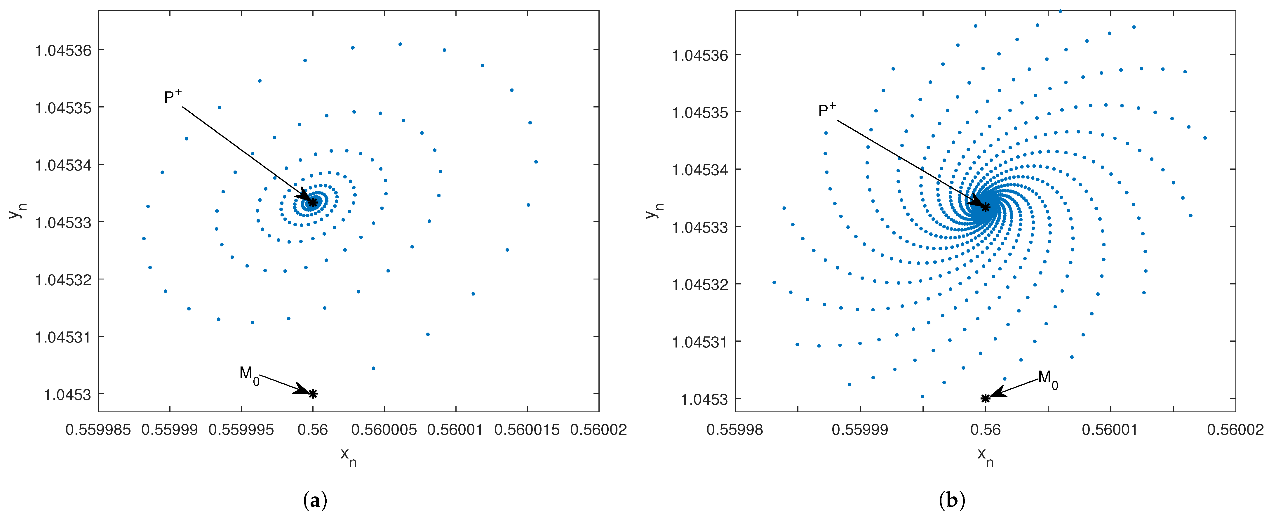
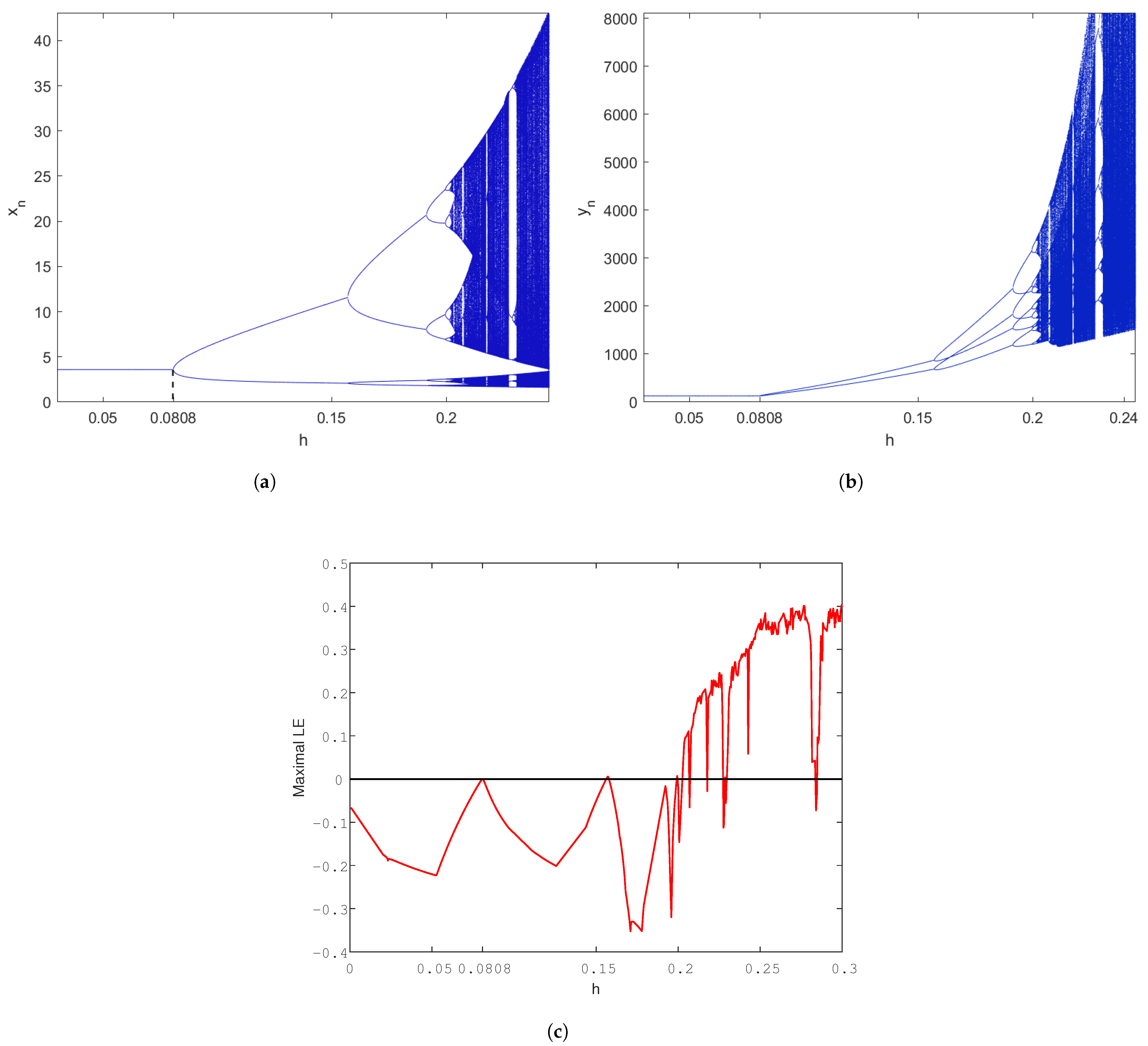
5. Numerical Computations and Discussion

This section presents the numerical computations of the obtained theoretical results. We also discuss the most important results obtained in this article.

Example 1.

In this example, we take $p=0.26$, $c=0.3$, $\alpha =0.5$, $h\in [0,1.4]$, and the initial conditions $M_0=(0.6,1.06)$, $M_1=(0.56,1.045)$. Then, System (6) undergoes a supercritical Neimark–Sacker bifurcation as h varies in a small neighborhood of

$$h^{\prime }={\left(\alpha +\frac{\alpha (p-c)}{c(p+c)}\right)}^{\frac{1}{\alpha }}=0.1451.$$

The bifurcation diagrams for $x_n$ and $y_n$ are shown in Figure 1a,b, respectively. Moreover, the maximum Lyapunov exponent (MLE) is plotted in Figure 1c. It is easy to observe that the equilibrium point of System (6) is locally asymptotically stable for $0<h<0.1451$. At $h=0.1451,$ the equilibrium point $P^{+}$ loses its property of local asymptotic stability. As a result, a closed invariant curve appears around the equilibrium point $P^{+}$ and inside the interval $h\in [0.1451,0.7901]$ due to the Neimark–Sacker bifurcation (see Figure 1d). Furthermore, when $h\in [0.7901,1.4]$, it is easy to observe the appearance of 10-, 20-, and 40-period orbits, quasi-periodic orbits, and attracting chaotic sets. In addition, the Jacobian matrix of System (6) under the above-mentioned values is given by

$$J\left(P^{+}\right)=\left(\begin{array}{cc}1.0544& -0.2187\\ 0.8533& 0.7714\end{array}\right),$$

whose eigenvalues are $\mu =0.9129-0.4081i$ and ${\mu }^{\prime }=0.9129+0.4081i.$ These eigenvalues definitely confirm that System (6) undergoes the Neimark–Sacker bifurcation at the point $P^{+}$. In Figure 2a–c, we present local magnifications of Figure 1a–c, respectively, whereas h changes in $[0.7901,1.013].$ It is easy to see that 10-, 20-, 40-period cycles appear when h passes through the value $h=0.7903$ in the chaotic region. Figure 3 is presented to illustrate the phase portraits of System (6) for different fixed values of h and the initial conditions $M_0$, $M_1$. When $h<h^{\prime }=0.1451$, System (6) has a positive equilibrium point that is locally asymptotically stable, as demonstrated in Figure 3a,b. Moreover, when the value of the bifurcation parameter h reaches $h^{\prime }=0.1451$, the stability of the system is lost, resulting in an attracting closed invariant curve ${\mathrm{\Lambda }}_s$ encircling the fixed point $P^{+}$ (see Figure 3c–e). All the orbits starting from the initial conditions both inside and outside of the invariant curve, with the exception of the equilibrium point $P^{+}$, approach ${\mathrm{\Lambda }}_s$ asymptotically (see Figure 3d,e). Some 10-, 20-, 40-period orbits are also plotted in Figure 4a–e. Finally, chaotic attractors are produced for $h=1.4$, as illustrated in Figure 4f.

Example 2.

We assume that $p=3.5$, $c=0.1$, $\alpha =0.25$, $h\in [0,0.245]$, and the initial condition $M_0=(3.2,129).$ Then, System (6) undergoes a period-doubling bifurcation when the bifurcation parameter $h^{-}=0.0808$. System (6) has a unique positive point $P^{+}$ at $(c,p,\alpha ,h^{-})=(0.1,3.5,0.25,0.0808).$ The Jacobian matrix of System (6) is given by

$$J\left(P^{+}\right)=\left(\begin{array}{cc}-1.0141& -0.0016\\ 15.3549& 0.7867\end{array}\right),$$

where its eigenvalues are $\mu =-1$ and ${\mu }^{\prime }=0.7726$, with $|{\mu }^{\prime }|\ne 1$. Hence, $(c,p,\alpha ,h^{-})=(0.1,3.5,0.25,0.0808)\in {\mathcal{B}}_{PD}$. The bifurcation diagrams of System (6) are shown in Figure 5a,b, while the maximum Lyapunov exponent (MLE) is plotted in Figure 5c. In Figure 5a,b, we observe that the fixed point $P^{+}$ of System (6) is asymptotically stable for $h<h^{-}=0.0808.$ This local stability can be also observed in Figure 5c, in which the system also loses its stability when $h=h^{-}$ via a period-doubling bifurcation. Further, when $h>h^{-}$, there is a period-doubling cascade in orbits of 2, 4, 8, 16, and 32 periods (see Figure 6a,b). The maximum Lyapunov exponents are computed, and the existence of chaotic regions in the parameter space is clearly depicted in Figure 5c.

6. Conclusions

This work has successfully investigated the qualitative behavior of System (3). In particular, System (3) has been discretized using the method of the piecewise constant argument and has been converted to a system of difference equations, as shown in System (6). Theorem 1 has shown that the equilibrium point $P^{+}$ becomes a sink, a source, a saddle, or non-hyperbolic under certain types of conditions. In Theorem 2, we have proved that System (10) undergoes a Neimark–Sacker bifurcation at the equilibrium point $P^{+}$ when the bifurcation parameter h varies in a small neighborhood of $h^{\prime }.$ This can be clearly seen in Figure 1a,b, which have been plotted with the values $p=0.26$, $c=0.3$, $\alpha =0.5$, $h\in [0,1.4]$, and $h^{\prime }=0.1451.$ In Figure 1c, we illustrate the maximum Lyapunov exponent (MLE). Furthermore, the first Lyapunov exponent for these parametric values is given by $\mathcal{L}=-0.000456<0$, which proves the correctness of Theorem 2. Our findings in Section 4.2 indicate that System (6) encounters a period-doubling bifurcation at the equilibrium point $P^{+}$ when the parameter h changes within a small neighborhood of ${\mathcal{B}}_{PD}$. Moreover, System (6) bifurcates from the fixed point $P^{+}$ to a two-periodic stable orbit if ${\mathcal{X}}_2>0$, while this system bifurcates from the fixed point $P^{+}$ to a two-periodic unstable orbit when ${\mathcal{X}}_2<0.$ The bifurcation diagrams of this system are plotted in Figure 5a,b with the parameter values $p=3.5$, $c=0.1$, $\alpha =0.25$, and $h\in [0,0.245]$ and the initial condition $M_0=(3.2,129).$ We can conclude that the proposed techniques are reliable and powerful and can be utilized to deal with other biological systems.

References

1. Patadiya, N.; Panchal, N.; Vaghela, V. A review on enzyme inhibitors. Int. Res. J. Pharm. 2021, 12, 60–66. [Google Scholar] [CrossRef]
2. Mohan, C.; Long, K.; Mutneja, M. An Introduction to Inhibitors and Their Biological Applications, 1st ed.; EMD Millipore Corporation: Burlington, MA, USA, 2013. [Google Scholar]
3. Gierer, A.; Meinhardt, H. A theory of biological pattern formation. Kybernetik 1972, 12, 30–39. [Google Scholar] [CrossRef] [PubMed]
4. Khan, A.Q.; Saleem, Z.; Ibrahim, T.F.; Osman, K.; Alshehri, F.M.; El-Moneam, M.A. Bifurcation and chaos in a discrete activator-inhibitor system. AIMS Math. 2022, 8, 4551–4574. [Google Scholar] [CrossRef]
5. Pasemann, G.; Flemming, S.; Alonso, S.; Beta, C.; Stannat, W. Diffusivity Estimation for Activator-Inhibitor Models: Theory and Application to Intracellular Dynamics of the Actin Cytoskeleton. J. Nonlinear Sci. 2020, 31, 59. [Google Scholar] [CrossRef]
6. Guo, L.; Shi, X.; Cao, J. Turing patterns of Gierer-Meinhardt model on complex networks. Nonlinear Dyn. 2021, 105, 899–909. [Google Scholar] [CrossRef]
7. Song, Y.; Yang, R.; Sun, G. Pattern dynamics in a Gierer-Meinhardt model with a saturating term. Appl. Math. Model. 2017, 46, 476–491. [Google Scholar] [CrossRef]
8. Chen, S.; Shi, J.; Chen, G.Z. Spatial pattern formation in activator-inhibitor models with nonlocal dispersal. Discrete Contin. Dyn. Syst. Ser. B 2021, 26, 1843–1866. [Google Scholar] [CrossRef]
9. Chen, S. Some properties for the solutions of a generalized Activator-Inhibitor model. Commun. Pure Appl. Anal. 2006, 5, 919–928. [Google Scholar] [CrossRef]
10. Ni, W.M.; Takagi, I.; Yanagida, E. Stability of least energy patterns of the shadow system for an activator-inhibitor model. Jpn. J. Indust. Appl. Math. 2001, 18, 259–272. [Google Scholar] [CrossRef]
11. Khan, A.Q.; Almatrafi, M.B. Two-dimensional discrete-time laser model with chaos and bifurcations. AIMS Math. 2023, 8, 6804–6828. [Google Scholar] [CrossRef]
12. Khan, A.Q.; Bukhari, S.A.H.; Almatrafi, M.B. Global dynamics, Neimark-Sacker bifurcation and hybrid control in a Leslie’s prey-predator model. Alex. Eng. J. 2022, 61, 11391–11404. [Google Scholar] [CrossRef]
13. Ross, R. The development of fractional calculus. Hist. Math. 1977, 4, 75–89. [Google Scholar] [CrossRef]
14. Miller, K.S.; Ross, B. An Introduction to the Fractional Calculus and Fractional Differential Equations; John Wiley & Sons: New York, NY, USA, 1993. [Google Scholar]
15. Riemann, B. Versuch Einer Allgemeinen Auffassung der Integration und Differentiation. Gesammelte Mathematische Werke und Wissenschaftlicher Nachlass; Teubner, Leipzig: New York, NY, USA, 1953. [Google Scholar]
16. Khalil, R.; Al Horani, M.; Yousef, A.; Sababheh, M. A new definition of fractional derivative. J. Comput. Appl. Math. 2014, 264, 65–70. [Google Scholar] [CrossRef]
17. Abdeljawad, T. On conformable fractional calculus. J. Comput. Appl. Math. 2014, 279, 57–66. [Google Scholar] [CrossRef]
18. Khalil, R. Flip and Neimark-Sacker Bifurcation in a Differential Equation With Piecewise Constant Arguments Model. J. Differ. Equ. Appl. 2017, 23, 763–778. [Google Scholar] [CrossRef]
19. Yousef, F.; Semmar, B.; Al Nasr, K. Incommensurate conformable-type three-dimensional Lotka-Volterra model: Discretization, stability, and bifurcation. Arab. J. Basic Appl. Sci. 2022, 29, 113–120. [Google Scholar] [CrossRef]
20. Yousef, F.; Semmar, B.; Al Nasr, K. Dynamics and simulations of discretized Caputo-conformable fractional-order Lotka-Volterra models. Nonlinear Eng. 2022, 11, 100–111. [Google Scholar] [CrossRef]
21. Wiener, J. Differential Equations with Piecewise Constant Delays, Trends in Theory and Practice of Nonlinear Differential Equations: Lecture Notes in Pure and Applied Math; Dekke: New York, NY, USA, 1984. [Google Scholar]
22. Berkal, M.; Navarro, J.F. Qualitative behavior of a two-dimensional discrete-time prey-predator model. Comp. Math. Methods 2021, 3, e1193. [Google Scholar] [CrossRef]
23. Liu, Y.; Li, X. Dynamics of a discrete predator-prey model with Holling-II functional response. Int. J. Biomath. 2021, 14, 2150068. [Google Scholar] [CrossRef]
24. Berkal, M.; Navarro, J.F. Qualitative study of a second order difference equation. Turkish J. Math. 2023, 47, 516–527. [Google Scholar] [CrossRef]
25. Carr, J. Application of Center Manifold Theory; Springer: New York, NY, USA, 1981. [Google Scholar]
26. Din, Q. Bifurcation analysis and chaos control in discrete-time glycolysis models. J. Math. Chem. 2018, 56, 904–931. [Google Scholar] [CrossRef]
27. Din, Q. Controlling chaos in a discrete-time prey-predator model with Allee effects. Int. J. Dyn. Control 2018, 6, 858–872. [Google Scholar] [CrossRef]
28. Din, Q.; Elsadany, A.A.; Ibrahim, S. Bifurcation analysis and chaos control in a second-order rational difference equation. Int. J. Nonlinear Sci. Numer. Simul. 2018, 19, 53–68. [Google Scholar] [CrossRef]
29. Kuznetsov, Y.A. Elements of Applied Bifurcation Theory; Springer: New York, NY, USA, 1997. [Google Scholar]
30. Wiggins, S. Dynamical Systems and Chaos; Springer Science and Business Media: Dordrecht, The Netherlands, 2003. [Google Scholar]
Figure 1. Bifurcation diagram and the maximum Lyapunov exponent for System (6) versus h [ 0 , 1.4 ] with the initial condition M 0 and bifurcation diagram in ( h x n y n ) space for h [ 0 , 0.1451 ] . (a) Bifurcation diagram for x n , (b) bifurcation diagram for y n , (c) maximum Lyapunov exponent (MLE), (d) bifurcation diagram in ( h x n y n ) space for h [ 0 , 0.1451 ] .
Fractalfract 07 00344 g001aFractalfract 07 00344 g001b
Figure 2. Bifurcation diagram and the maximum Lyapunov exponent for System (6) versus h [ 0.7901 , 1.013 ] with the initial condition M 0 . (a) Bifurcation diagram for x n , (b) bifurcation diagram for y n , (c) maximum Lyapunov exponent (MLE).
Fractalfract 07 00344 g002aFractalfract 07 00344 g002b
Figure 3. Phase portraits for h [ 0 , 0.7901 ] of System (4). (a) Phase portrait for h = 0.049 , (b) phase portrait for h = 0.13 , (c) phase portrait for h = h = 0.1451 , (d) phase portrait for h = 0.148 , (e) phase portrait for h = 0.151 , (f) phase portrait for h = 0.23 .
Fractalfract 07 00344 g003aFractalfract 07 00344 g003b
Figure 4. Phase portraits for h [ 0.7901 , 1.4 ] of System (4). (a) Phase portrait for h = 0.84 , (b) phase portrait for h = 0.94 , (c) phase portrait for h = 1.009 , (d) phase portrait for h = 1.1 , (e) phase portrait for h = 1.15 , (f) phase portrait for h = 1.4 .
Fractalfract 07 00344 g004
Figure 5. Bifurcation diagrams and the maximum Lyapunov exponent for System (6) with the initial condition M 0 . (a) Bifurcation diagram for x n with h [ 0 , 0.245 ] , (b) bifurcation diagram for y n with h [ 0 , 0.245 ] , (c) maximum Lyapunov exponent (MLE) with h [ 0 , 0.3 ] .
Fractalfract 07 00344 g005
Figure 6. Bifurcation diagrams for System (6) with h [ 0.081 , 0 , 22 ] . (b) Bifurcation diagram for x n , (a) bifurcation diagram for y n .
Fractalfract 07 00344 g006
Disclaimer/Publisher’s Note: The statements, opinions and data contained in all publications are solely those of the individual author(s) and contributor(s) and not of MDPI and/or the editor(s). MDPI and/or the editor(s) disclaim responsibility for any injury to people or property resulting from any ideas, methods, instructions or products referred to in the content.