Article

Input-Output Finite-Time Stability of Fractional-Order Switched Singular Systems with D-Perturbation

School of Mathematics and Computer Science, Shanxi Normal University, Taiyuan 030032, China
*
Author to whom correspondence should be addressed.
Fractal Fract. 2023, 7(4), 341; https://doi.org/10.3390/fractalfract7040341
Submission received: 15 March 2023 / Revised: 6 April 2023 / Accepted: 18 April 2023 / Published: 20 April 2023

Abstract

:
The objective of this paper focuses on the stability analysis of the input-output finite-time for a class of fractional-order switched singular systems (FOSSS) with D-perturbation. By using the Φ-dependent average dwell time (ΦDADT) approach together with the multiple Lyapunov functions method, some sufficient conditions are derived for the considered system to ensure its input-output finite-time stability in terms of linear matrix inequalities. Then, the output feedback controller is designed to ensure the closed-loop system is input-output finite-time stable. Finally, a numerical example illustrates the superiority of the proposed method.

1. Introduction

Recently, fractional calculus has drawn a great deal of attention and interest from science and engineering fields due to its significant properties, such as diffusive realization [1], lung tissue viscoelasticity [2], diffusive representation [3], heat conduction [4], robust control [5], electric energy consumption [6], and chaotic systems [7]. Over the years of development, the fractional-order positive switched system (FOPSS) has obtained some meaningful results in an infinite time interval [8,9,10,11]. Among them, the works [8,9] investigate the controllability and switching control for FOPSS with the fixed switching sequence and state-dependent switching, respectively. The Lyapunov stability and robust stabilizing state feedback controller design of fractional-order nonlinear systems are presented in [10,11], respectively. Recently, finite-time stability (FTS) analysis of FOPSS has become a research hotspot because of its theoretical and practical importance. FTS means that the solutions of the system do not exceed a certain bound during a specified time interval. It is a more practical concept, which is helpful to study the behavior of the system during a finite short interval. Therefore, the stability analysis of FOPSS is considered in a finite time interval [12,13,14,15,16,17,18]. In the literature [12], the FTS problem of FOPSS is studied based on the average dwell time (ADT) approach. In the literature [13] and the literature [14], the FTS and finite-time control problem for certain and uncertain fractional-order positive impulsive switched systems are investigated using the ADT and mode-dependent average dwell time (MDADT) approach, respectively. In the literature [15], the impulsive observer design of FOPSS via the MDADT approach is studied. FTS and finite-time boundedness (FTB) of FOPSS with 0 < α < 1 are studied by employing the ADT approach [16]. The consensus problem of fractional-order multiagent systems (FOMS) is investigated via sampled-data event-triggered control [17]. The consensus problem of leader-following for FOMS is addressed [18]. A class of fractional-order positive switched continuous-time systems is focused [19]. To ensure good system performance, in recent years, the stability problem of robust finite-time guaranteed cost control for FOPSS with impulsive and time-varying delay was studied [20]. The guaranteed cost and finite-time event-triggered control problem of FOPSS are considered via the ADT approach [21]. Guaranteed cost and finite-time non-fragile control problems of FOPSS with impulsive moments and asynchronous switching are discussed under the ADT approach [22]. It is noteworthy that the FTS analysis of FOPSS has not been studied by the ΦDADT approach which is more general than the ADT and MDADT ones [23]. It motivates us to do this in this paper.
Moreover, many results and concepts of FOPSS have been extended to FOSSS, for example [24,25]. In the literature [24], the FTS of FOSSS with delay is studied by “inf-sup” the method and Laplace transform based on Mittag–Leffler functions and tractable matrix inequalities. In the literature [25], the robust control problem of FOSSS is proposed by using the linear matrix inequalities (LMIs) method and generalized singular value decomposition. Very recently, the literature [26] addressed the input-output finite-time stability (IO-FTS) of FOSSS with 0 < α < 1 .
Most of these conclusions mentioned above are undisturbed, in reality, almost all the physical systems contain perturbations because of the existence of hardware errors, such as modeling errors and fluctuation. A typical perturbation for positive switched systems is called D-perturbation. Recently, several works have obtained related conclusions about D-perturbation [27,28,29]. The robust stability of positive switched linear systems with D-perturbation and time-varying delay is considered [27], and the guaranteed cost finite-time boundedness of positive switched nonlinear systems with D-perturbation and time-varying is studied [28]. In the literature [29], the problem of guaranteed cost finite-time control for fractional-order nonlinear positive switched systems is investigated. Up to now, few results consider the IO-FTS for FOSSS in the presence of D-perturbation. This is another motivation for this study.
This paper focuses on the IO-FTS for a class of FOSSS with D-perturbation. The main three contributions of this paper are as follows: (i) Regularity and impulse-free properties of FOSSS with D-perturbation are given. (ii) By using the ΦDADT approach together with the multiple Lyapunov functions method, sufficient conditions are derived for the considered systems which ensure the input-output finite-time stable in terms of linear matrix inequalities. (iii) The output feedback controller is designed to ensure the closed-loop system is input-output finite-time stable.
The rest of the paper is organized as follows. In Section 2, the basic inequalities are given, which contain C p , Young’s, and Grownwall–Bellman inequalities. Moreover, necessary definitions of fractional-order calculus are presented. In Section 3, the input-output stability criterion for FOSSS is given. A numerical example illustrates the superiority of the proposed results in Section 4. Lastly, the results are summarized in Section 5.

2. Problem Formulation and Preliminaries

Notations: Z * ( R and C ) stands for the set of positive integers (real and complex numbers). R n stands for real Euclidean space with n-dimension. R n × m signifies the space of n × m real matrices. A T and A 1 stand for the transpose of and inverse of matrix A. Rank ( X ) is the rank of the matrix X. I means that the identity matrix. Matrix D [ D ̲ , D ¯ ] signifies that d i j [ d ̲ i j , d ¯ i j ] . A 0 ( , , ) signifies that a i j > 0 ( < 0 , 0 , 0 ) , which is applicable to a vector. A > B ( A < B , A B , A B ) means that A B is a positive-definite (negative-definite, positive-semidefinite, and negative-semidefinite) matrix.

2.1. Fractional-Order Calculus

In this subsection, some basic knowledge and definitions of fractional-order calculus are introduced.
The uniform formula of the fractional integral of order β of a given function ( s ) on [ s 0 , s ] is given as
s 0 D s β ( s ) = 1 Γ ( β ) s 0 s ( τ ) ( s τ ) 1 β d τ ,
where 0 < β < 1 , and Γ ( β ) = 0 e s s β 1 d s represents the Gamma function.
Then, the Caputo fractional derivative is given as follows:
D s β s 0 C ( s ) = 1 Γ ( 1 β ) s 0 s ( τ ) ( s τ ) β d τ ,
where D s β s 0 C stands for Caputo fractional derivatives of order β of function ( s ) on [ s 0 , s ] . In this paper, we use Caputo fractional-order operators as our main tool.
Next, some lemmas and useful inequalities are given for further study.
Lemma 1
([26]). Suppose that 0 < β < 1 , let x ( s ) R n be a continuous and differentiable vector function, H R n × n , H 0 , then for any time instant s 0 , the following inequality holds
1 2 s 0 C D s β [ x T ( s ) H x ( s ) ] x T ( s ) H s 0 C D s β x ( s ) .
Lemma 2
([30]). Let a ( s ) , b ( s ) and ( s ) be real-valued piecewise-continuous functions. If a ( s ) is non-negative and ( s ) satisfies
( s ) a ( s ) + s 0 s b ( t ) ( t ) d t ,
then
( s ) a ( s ) + s 0 s a ( t ) b ( t ) exp t s b ( r ) d r d t .
In particular, if a ( s ) is a constant, then it holds
( s ) a ( s ) exp ( s 0 s b ( t ) d t ) .
Lemma 3
([12]). ( C p inequality) For any positive real numbers x 1 , x 2 , , x m ,
m = 1 N x m β N 1 β ( m = 1 N x m ) β , ( 0 < β < 1 ) .
Lemma 4
([12]). (Young’s inequality) If , z , p and q are all real numbers, p , q > 0 , then
p z q p p + q p + q + q p + q z p + q .
Lemma 5
([31]). Let A ¯ R n × n , then A ¯ is nonsingular if and only if there exists a nonsingular matrix X R n × n such that
A ¯ X + X T A ¯ T < 0 ,
where A ¯ = D A .

2.2. Fractional-Order Switched Singular Systems

Consider the following FOSSS:
E ς ( s ) s 0 C D s β x ( s ) = D 1 A ς ( s ) x ( s ) + D 2 G ς ( s ) u ( s ) + D 3 B ς ( s ) ω ( s ) , y ( s ) = D 4 C ς ( s ) x ( s ) ,
where 0 < β < 1 . s 0 = 0 , x ( s 0 ) = 0 and x ( s ) R n represent the initial time, initial state, and system state, respectively. u ( s ) R m and y ( s ) R p are the control input and output, respectively. ς ( s ) : [ s 0 , + ) F m = { 1 , 2 , , M } is the switching signal. Letting O = { 1 , 2 , , N } , N M . Definite mapping Φ : F m O is an epimorphism operator. Set Φ γ = { p F m | Φ ( p ) = γ O } . Perturbations D i [ D ¯ i , D ̲ i ] ( i = 1 , 2 , 3 , 4 ) with D ¯ i D ̲ i 0 where matrices D ¯ i , D ̲ i are all diagonal. For p F m , E p , A p , G p , B p and C p R n × n are known constant matrices and rank ( E p ) = r p n . ω ( s ) R q represents the exogenous disturbance input with ω ( t ) W ( S , F , d ) : = { ω ( · ) L [ 0 , S ] : ω T ( s ) F ω ( s ) d } where F = F T > 0 .
In the following development, let A ¯ p = D 1 A p , G ¯ p = D 2 G p , B ¯ p = D 3 B p and C ¯ p = D 4 C p , A ¯ ¯ p = D ¯ 1 A p , G ¯ ¯ p = D ¯ 2 G p , B ¯ ¯ p = D ¯ 3 B p , C ¯ ¯ p = D ¯ 4 C p .
The p-th subsystem of system (3) is considered as follows:
E p s 0 C D s β x ( s ) = A ¯ p x ( s ) + G ¯ p u ( s ) + B ¯ p ω ( s ) .
Definition 1
([32]). System (4) is said to be regular if there exists a scalar k C such that det ( k β E p A ¯ p ) 0 holds.
Definition 2
([32]). System (4) is said to be impulse-free if deg(det ( k E p A ¯ p ) ) = rank ( E p ) , k C .
Definition 3
([26]). System (3) is called regular and impulse-free if each singular subsystem (4) is regular and impulse-free.
Lemma 6
([32]). For system (4), it is always possible to find two nonsingular matrices U p , Z p R n × n such that ( E p , A ¯ p ) takes the following decomposition form
U p E p Z p = I r 0 0 0 , U p A ¯ p Z p = A ¯ p 11 A ¯ p 12 A ¯ p 21 A ¯ p 22 .
For the above form, system (4) is said to be regular and impulse-free if A ¯ p 22 is nonsingular.
Definition 4
([26]). If the state of system (3) at every switching instant has a consistent initial value of the next active subsystem, then the switching is called consistent switching for system (3).
However, x ( s l ) may not be a consistent initial value for the activated system after the switch. Therefore, to guarantee the consistent switching of system (3), the projector is given as follows:
Π p = Z p I r 0 A ¯ p 22 1 A ¯ p 21 0 Z p 1 .
Assumption A1
([33]). If the state of the system (3) satisfies
x ( s l ) = Π p x ( s l ) ,
where x ( s l ) stands the state before the switching s l , then the state jump behaviors can be evaluated by the consistency projector Π p in (5).
Definition 5
([23]). Let N ς Φ γ ( s , s 0 ) be the sum of switching numbers of subsystems Φ γ being activated over [ s 0 , s ] , and S Φ γ ( s , s 0 ) represents total running time of subsystems Φ γ over [ s 0 , s ] , assume that there exist two constants N 0 Φ γ 0 and τ a Φ γ > 0 , γ O , such that
N ς Φ γ ( s , s 0 ) N 0 Φ γ + S Φ γ ( s , s 0 ) τ a Φ γ , s s 0 0 ,
where N 0 Φ γ is called the chatter bounds. Then, τ a Φ γ is called ΦDADT of ς ( s ) .
Remark 1.
The definitions of ADT and MDADT can be obtained by taking O = { 1 } and O = F m in Definition 5.
Definition 6
([26]). Given a positive scalar S , a class of input signal W defined over [ 0 , S ] and a positive definite matrix Q, then system (3) is said to be input-output finite-time stable concerning ( W , Q , S ) if the following condition holds:
ω ( · ) W y T ( s ) Q y ( s ) < 1 , s [ 0 , S ] .

3. Results

3.1. Input-output Finite-Time Stability

In this subsection, the input-output FTS of system (3) is considered with u = 0 .
Theorem 1.
Consider system (3) with u = 0 . Given constants λ γ > 0 and μ γ > 1 , γ O , for p , q F m , p q , assume that there exist nonsingular matrices H p , such that
H p T A ¯ ¯ p + A ¯ ¯ p T H p λ γ E p T H p H p T B ¯ ¯ p B ¯ ¯ p T H p λ γ F < 0 ,
Π p T E p T H p Π p μ γ E q T H q ,
C ¯ ¯ p T Q C ¯ ¯ p E p T H p = H p T E p ,
then system (3) with u = 0 is regular, impulse-free, and input-output finite-time stable concerning ( W , Q , S ) for all s [ 0 , S ] with the ΦDADT satisfying
τ a Φ γ > τ a Φ γ * = η ϕ ln d ,
where η = S γ ln μ γ + λ γ ( 1 β ) S γ Γ ( β + 1 ) , ϕ = N 0 Φ γ ln μ γ + λ γ ( 1 β ) ( N 0 Φ γ + 1 ) Γ ( β + 1 ) + λ γ β S γ Γ ( β + 1 ) .
Proof.
For p F m , let
U p T H p Z p = H p 11 H p 12 H p 21 H p 22 .
By Lemma 6 and (11), we can obtain
Z p T E p T H p Z p = Z p T E p T U p T U p T H p Z p = H p 11 H p 12 0 0 0 ,
Z p T H p T E p Z p = Z p T H p T U p 1 U p E p Z p = H p 11 T 0 H p 12 T 0 0 ,
with E p T H p = H p T E p .
Then, it is obvious that (13) satisfies H p 12 = 0 , H p 11 = H p 11 T 0 . Therefore,
U p T H p Z p = H p 11 0 H p 21 H p 22 ,
where H p 11 and H p 22 are nonsingular because H p is nonsingular. It follows from (9) that
Z p T H p T A ¯ ¯ p Z p + Z p T A ¯ ¯ p T H p T Z p λ γ Z p T E p T H p Z p = Z p T H p T U p 1 U p A ¯ ¯ p Z p + Z p T A ¯ ¯ p T U p T U p T H p Z p λ γ Z p T H p T U p 1 U p E p Z p = 🟉 🟉 🟉 A ¯ ¯ p 22 T H p 22 + H p 22 T A ¯ ¯ p 22 < 0 ,
where 🟉 stands for some matrix blocks that we do not care about. It is easily obtained from (17) that A ¯ ¯ p 22 T H p 22 + H p 22 T A ¯ ¯ p 22 < 0 . Then, it further can be deduced that A ¯ p 22 T H p 22 + H p 22 T A ¯ p 22 < 0 . By applying Lemma 5, it follows that A ¯ p 22 is nonsingular. Further, from Lemma 6, we conclude that system (4) with u = 0 is regular and impulse-free. Moreover, by using Definition 3, the properties of the regularity and impulse-free of system (3) with u = 0 are ensured.
Next, the IO-FTS of system (3) with u = 0 is proved.
The multiple Lyapunov functions are constructed as follows:
V ς ( s ) = V ς ( s ) ( s , x ( s ) ) = x T ( s ) E ς ( s ) T H ς ( s ) x ( s ) + d .
It is obvious that V ς ( s ) > 0 . Denote 0 s 0 < s 1 < as a switching sequence. Taking the fractional-order derivative of (18), for s [ s l , s l + 1 ) , one can obtain
D s β s 0 C V ς ( s ) ( s , x ( s ) ) 2 x T ( s ) E ς ( s ) T H ς ( s ) s 0 C D s β x ( s ) = 2 x T ( s ) H ς ( s ) T E ς ( s ) s 0 C D s β x ( s ) = 2 x T ( s ) H ς ( s ) T ( A ¯ ς ( s ) x ( s ) + B ¯ ς ( s ) ω ( s ) ) 2 x T ( s ) H ς ( s ) T ( A ¯ ¯ ς ( s ) x ( s ) + B ¯ ¯ ς ( s ) ω ( s ) ) = x T ( s ) ( H ς ( s ) T A ¯ ¯ ς ( s ) + A ¯ ¯ ς ( s ) T H ς ( s ) ) x ( s ) + x T ( s ) H ς ( s ) T B ¯ ¯ ς ( s ) ω ( s ) + ω T ( s ) B ¯ ¯ ς ( s ) T H ς ( s ) x ( s ) = x ( s ) ω ( s ) T H ς ( s ) T A ¯ ¯ ς ( s ) + A ¯ ¯ ς ( s ) T H ς ( s ) H ς ( s ) T B ¯ ¯ ς ( s ) B ¯ ¯ ς ( s ) T H ς ( s ) 0 x ( s ) ω ( s ) < x ( s ) ω ( s ) T λ γ E ς ( s ) T H ς ( s ) 0 0 λ γ F x ( s ) ω ( s ) = λ γ x T ( s ) E ς ( s ) T H ς ( s ) x ( s ) + λ γ ω T ( s ) F ω ( s ) = λ γ ( x T E ς ( s ) T H ς ( s ) x ( s ) + d ) = λ γ V ς ( s ) ( s , x ( s ) ) .
By taking the fractional integral operator D s β s l C to both sides of (19) on the interval [ s l , s ) , for s [ s l , s l + 1 ) , one can further obtain
V ς ( s ) ( s , x ( s ) ) < V ς ( s l ) ( s l , x ( s l ) ) + λ γ Γ ( β ) s l s ( s τ ) β 1 V ς ( s l ) ( τ , x ( τ ) ) d τ .
With the help of Lemma 2, for s [ s l , s l + 1 ) , it follows that
V ς ( s ) ( s , x ( s ) ) < V ς ( s l ) ( s l , x ( s l ) ) exp { λ Φ ς ( s l ) Γ ( β ) s l s ( s τ ) β 1 d τ } = V ς ( s l ) ( s l , x ( s l ) ) exp { λ Φ ς ( s l ) β Γ ( β ) ( s s l ) β } = V ς ( s l ) ( s l , x ( s l ) ) exp { λ Φ ς ( s l ) Γ ( β + 1 ) ( s s l ) β } .
For s [ s l , s l + 1 ) , together with Assumption 1 and (10), this implies
V ς ( s l ) ( s l , x ( s l ) ) = x T ( s l ) E ς ( s l ) T H ς ( s l ) x ( s l ) + d = x T ( s l ) Π ς ( s l ) T E ς ( s l ) T H ς ( s l ) Π ς ( s l ) x ( s l ) + d μ Φ ς ( s l ) V ς ( s l ) ( s l , x ( s l ) ) .
According to exp { λ Φ ς ( s l ) Γ ( β + 1 ) ( s s l ) β } > 0 , one has
V ς ( s ) ( s , x ( s ) ) < μ Φ ς ( s l ) V ς ( s l ) ( s l , x ( s l ) ) exp { λ Φ ς ( s l ) Γ ( β + 1 ) ( s s l ) β } < μ Φ ς ( s l ) V ς ( s l 1 ) ( s l 1 , x ( s l 1 ) ) exp { λ Φ ς ( s l 1 ) Γ ( β + 1 ) ( s l s l 1 ) β + λ Φ ς ( s l ) Γ ( β + 1 ) ( s s l ) β } < μ Φ ς ( s l ) μ Φ ς ( s l 1 ) V ς ( s l 1 ) ( s l 1 , x ( s l 1 ) ) exp { λ Φ ς ( s l 1 ) Γ ( β + 1 ) ( s l s l 1 ) β + λ Φ ς ( s l ) Γ ( β + 1 ) ( s s l ) β } < < i = 1 l μ Φ ς ( s i ) V ς ( s 0 ) ( s 0 , x ( s 0 ) ) exp { λ Φ ς ( s 0 ) Γ ( β + 1 ) ( s 1 s 0 ) β + λ Φ ς ( s 1 ) Γ ( β + 1 ) ( s 2 s 1 ) β + + λ Φ ς ( s l ) Γ ( β + 1 ) ( s l + 1 s l ) β } .
From Lemmas 3 and 4, for s [ 0 , S ] , we have
V ς ( s ) ( s , x ( s ) ) < V ς ( s 0 ) ( s 0 , x ( s 0 ) ) γ = 1 N μ γ N γ exp { 1 Γ ( β + 1 ) γ = 1 N λ γ ς ( s l ) Φ γ ( s l + 1 s l ) β } < V ς ( s 0 ) ( s 0 , x ( s 0 ) ) exp { γ = 1 N ln μ γ N γ + γ = 1 N λ γ Γ ( β + 1 ) ( N γ + 1 ) 1 β S γ β } < V ς ( s 0 ) ( s 0 , x ( s 0 ) ) exp { γ = 1 N ln μ γ N γ + γ = 1 N λ γ Γ ( β + 1 ) [ ( 1 β ) ( N γ + 1 ) + β S γ ] } < V ς ( s 0 ) ( s 0 , x ( s 0 ) ) exp { γ = 1 N [ ( N 0 Φ γ + S γ τ a Φ γ ) ln μ γ + λ γ Γ ( β + 1 ) ( ( 1 β ) ( N 0 Φ γ + S γ τ a Φ γ + 1 ) + β S γ ) ] } < V ς ( s 0 ) ( s 0 , x ( s 0 ) ) exp { γ = 1 N [ ln μ γ τ a Φ γ S γ + λ γ ( 1 β ) Γ ( β + 1 ) S γ τ a Φ γ + N 0 Φ γ ln μ γ + λ γ ( 1 β ) N 0 Φ γ Γ ( β + 1 ) + λ γ ( 1 β ) Γ ( β + 1 ) + λ γ β S γ Γ ( β + 1 ) ] } < V ς ( s 0 ) ( s 0 , x ( s 0 ) ) < exp { γ = 1 N [ 1 τ a Φ γ ( S γ ln μ γ + λ γ ( 1 β ) Γ ( β + 1 ) S γ ) + N 0 Φ γ ln μ γ + λ γ ( 1 β ) N 0 Φ γ Γ ( β + 1 ) + λ γ ( 1 β ) Γ ( β + 1 ) + λ γ β S γ Γ ( β + 1 ) ] } < V ς ( s 0 ) ( s 0 , x ( s 0 ) ) exp { γ = 1 N ( 1 τ a Φ γ η + ϕ ) } ,
where N γ N ς Φ γ ( S , 0 ) , S γ S Φ γ ( S , 0 ) . Taking the zero initial condition x ( 0 ) = 0 , then V ς ( 0 ) ( 0 , x ( 0 ) ) = x T ( 0 ) E ς ( 0 ) T H ς ( 0 ) x ( 0 ) + d = d , we have
y T ( s ) Q y ( s ) = x T ( s ) C ¯ ς ( s ) T Q C ¯ ς ( s ) x ( s ) x T ( s ) C ¯ ¯ ς ( s ) T Q C ¯ ¯ ς ( s ) x ( s ) x T ( s ) E ς ( s ) T H ς ( s ) x ( s ) + d = V ς ( s ) ( s , x ( s ) ) < d exp { γ = 1 N ( 1 τ a Φ γ η + ϕ ) } .
Substituting(12) into (25), we can obtain
y T ( s ) Q y ( s ) < 1 .
From Definition 6, it can be concluded that the system (3) with u = 0 is regular, impulse-free, and input-output finite-time stable about ( W , Q , S ) . Thus, the proof is completed. □
Remark 2.
The conditions (9–11) are only sufficient for the conclusion of Theorem 1. In some cases, they may not be feasible. To guarantee the maximum solvability of LMIs (9–11), it is often necessary to first select a set of sufficiently large μ γ and sufficiently small λ γ , which can ensure that H p has a large degree of freedom. If LMIs (9–11) are feasible under such μ γ and λ γ conditions, it can gradually reduce μ γ and increase λ γ to achieve better ΦDADT τ a Φ γ * design.
When O = { 1 } ( O = F m ), we can obtain the ADT (MDADT) results of FOPSSS.
Corollary 1.
Consider system (3) with u = 0 . For constants λ > 0 and μ > 1 , p F m , p q , assume that there exist nonsingular matrix H p , such that
H p T A ¯ ¯ p + A ¯ ¯ p T H p λ E p T H p H p T B ¯ ¯ p B ¯ ¯ p T H p λ F < 0 ,
Π p T E p T H p Π p μ E q T H q ,
C ¯ ¯ p T Q C ¯ ¯ p E p T H p = H p T E p ,
then system (3) with u = 0 is regular, impulse-free, and input-output finite-time stable concerning ( W , Q , S ) for all s [ 0 , S ] with the ADT satisfying
τ a > τ a * = η ϕ ln d ,
where η = S ln μ + λ ( 1 β ) S Γ ( β + 1 ) , ϕ = N 0 ln μ + λ ( 1 β ) ( N 0 + 1 ) Γ ( β + 1 ) + λ β S Γ ( β + 1 ) .
Proof.
The corresponding result can be obtained by taking O = { 1 } . So we omit here. □
Corollary 2.
Consider system (3) with u = 0 . For constants λ p > 0 and μ p > 1 , p F m , p q , assume that there exist nonsingular matrices H p , such that
H p T A ¯ ¯ p + A ¯ ¯ p T H p λ p E p T H p H p T B ¯ ¯ p B ¯ ¯ p T H p λ p F < 0 ,
Π p T E p T H p Π p μ p E q T H q ,
C ¯ ¯ p T Q C ¯ ¯ p E p T H p = H p T E p ,
then system (3) with u = 0 is regular, impulse-free, and input-output finite-time stable concerning ( W , Q , S ) for all s [ 0 , S ] with the MDADT satisfying
τ a p > τ a p * = η ϕ ln d ,
where η = S p ln μ p + λ p ( 1 β ) S p Γ ( β + 1 ) , ϕ = N 0 p ln μ p + λ p ( 1 β ) ( N 0 p + 1 ) Γ ( β + 1 ) + λ β S p Γ ( β + 1 ) .
Proof.
The corresponding result can be obtained by taking O = F m . So we omit here. □
Remark 3.
It can easily be known that Theorem 1 can cover Corollaries 1 and 2. Therefore, our proposed approach is a more general way to study the stability analysis of a class of FOSSS with 0 < β < 1 .
Remark 4.
Letting O = { 1 } . If D 1 = D 2 = D 3 = D 4 = I and u = 0 , then Theorem 1 can be transformed into Theorem 1 of the literature [26].

3.2. Input-Output Finite-Time Stabilization

In this section, an output feedback controller for system (3) is designed as follows:
u ( s ) = K ς ( s ) y ( s ) ,
the corresponding closed-loop system is given by
E ς ( s ) s 0 C D s β x ( s ) = A ^ ς ( s ) x ( s ) + B ¯ ς ( s ) ω ( s ) , y ( t ) = C ¯ ς ( s ) x ( s ) ,
where A ^ ς ( s ) = A ¯ ς ( s ) + G ¯ ς ( s ) K ς ( s ) C ¯ ς ( s ) .
Theorem 2.
Consider system (36). For constants λ γ > 0 and μ γ > 1 , γ O , for p , q F m , p q , assume that there exist nonsingular matrices X p , L p , p F m , such that
X p T A ¯ ¯ p T + A ¯ ¯ p X p + C ¯ ¯ p T L p T G ¯ ¯ p T + G ¯ ¯ p L p C ¯ ¯ p λ γ X p T E p T B ¯ ¯ p B ¯ ¯ p T λ γ F < 0 ,
X p T C ¯ ¯ p T Q C ¯ ¯ p X p E p X p = X p T E p T
and (10) hold, where H p = X p 1 , and the output feedback controller u ( s ) = K p y ( s ) = L p X p 1 y ( s ) , then system (36) is regular, impulse-free, and input-output finite-time stable about ( W , Q , S ) for all s [ 0 , S ] with the ΦDADT satisfying (12).
Proof.
Multiplying (38) by X p T on the left and by X p 1 on the right, we have
C ¯ ¯ p T Q C ¯ ¯ p H p T E p = E p T H p .
Further, pre-multiplying and post-multiplying (37) by
X p T 0 0 I , X p 1 0 0 I
respectively, one gets
A ¯ ¯ p T H p + H p T A ¯ ¯ p + C ¯ ¯ p T K p T G ¯ ¯ p T H p + H p T G ¯ ¯ p K p C ¯ ¯ p λ γ E p T H p H p T B ¯ ¯ p B ¯ ¯ p T H p λ γ F < 0 .
Then (41) can be rewritten as
A ^ ¯ p T H p + H p T A ^ ¯ p λ γ E T H p H p T B ¯ ¯ p B ¯ ¯ p T H p λ γ F < 0 ,
where A ^ ¯ ς ( s ) = A ¯ ¯ ς ( s ) + G ¯ ¯ ς ( s ) K ς ( s ) C ¯ ¯ ς ( s ) . Replacing A ¯ ¯ p in (9) with A ^ ¯ p . Similar to Theorem 1, we easily derived that the corresponding closed-loop system (36) is regular, impulse-free, and input-output finite-time stable in regard to ( W , Q , S ) for all s [ 0 , S ] with the switching signal (12). Thus, the proof is completed. □
Similar to Section 3.1, the following two corollaries can be obtained from Theorem 2.
Corollary 3.
Consider system (36). For constants λ > 0 and μ > 1 , for p , q F m , p q , assume that there exist nonsingular matrices X p , L p , such that
X p T A ¯ ¯ p T + A ¯ ¯ p X p + C ¯ ¯ p T L p T G ¯ ¯ p T + G ¯ ¯ p L p C ¯ ¯ p λ X p T E p T B ¯ ¯ p B ¯ ¯ p T λ F < 0 ,
and (28), (38) hold, where H p = X p 1 , and the output feedback controller u ( s ) = K p y ( s ) = L p X p 1 y ( s ) , then system (36) is regular, impulse-free and input-output finite-time stable in regard to ( W , Q , S ) for all s [ 0 , S ] with the ADT satisfying (30).
Proof.
It can obtain this result directly by taking O = { 1 } . □
Corollary 4.
Consider the system (36). For constants λ p > 0 and μ p > 1 , for p , q F m , p q , assume that there exist nonsingular matrices X p , L p , such that
X p T A ¯ ¯ p T + A ¯ ¯ p X p + C ¯ ¯ p T L p T G ¯ ¯ p T + G ¯ ¯ p L p C ¯ ¯ p λ p X p T E p T B ¯ ¯ p B ¯ ¯ p T λ p F < 0 ,
and (32), (38) hold, where H p = X p 1 , and the output feedback controller u ( s ) = K p y ( s ) = L p X p 1 y ( s ) , then system (36) is regular, impulse-free, and input-output finite-time stable in regard to ( W , Q , S ) for all s [ 0 , S ] with the MDADT satisfying (34).
Proof.
It can obtain this result directly by taking O = F m . □
Remark 5.
In fact, the condition (38) is not the standard LMIs due to the existence of product between matrices X p , which implies that, given the conditions in Theorem 2, Corollaries 3 and 4 cannot be solved by using the LMI control toolbox in Matlab. Therefore, the feasible corollaries are given by Schur complements.
Corollary 5.
Consider the system (36). For constants λ γ > 0 and μ γ > 1 , γ O , for p , q F m , p q , assume that there exist nonsingular matrices X p , L p , p F m , such that
E p X p = X p T E p T ,
E p X p X p T C ¯ ¯ p T C ¯ ¯ p X p Q 1 0
and (10), (37) hold, where H p = X p 1 , and the output feedback controller u ( s ) = K p y ( s ) = L p X p 1 y ( s ) , then system (36) is regular, impulse-free and input-output finite-time stable in regard to ( W , Q , S ) for all s [ 0 , S ] with the ΦDADT satisfying (12).
Proof.
It can obtain this result directly by taking O = { 1 , 2 } . □
Corollary 6.
Consider system (36). For constants λ > 0 and μ > 1 , for p , q F m , p q , assume that there exist nonsingular matrices X p , L p , such that (28), (43), (45) and (46) hold, where H p = X p 1 , and the output feedback controller u ( s ) = K p y ( s ) = L p X p 1 y ( s ) , then system (36) is regular, impulse-free and input-output finite-time stable in regard to ( W , Q , S ) for all s [ 0 , S ] with the ADT satisfying (30).
Proof.
It can obtain this result directly by taking O = { 1 } . □
Corollary 7.
Consider system (36). For constants λ p > 0 and μ p > 1 , for p , q F m , p q , assume that there exist nonsingular matrices X p , L p , such that (32) and (44)–(46) hold, where H p = X p 1 , and the output feedback controller u ( s ) = K p y ( s ) = L p X p 1 y ( s ) , then system (36) is regular, impulse-free and input-output finite-time stable in regard to ( W , Q , S ) for all s [ 0 , S ] with the MDADT satisfying (34).
Proof.
It can obtain this result directly by taking O = F m . □
Remark 6.
Compared with traditional systems, the stability analysis of FOSSS with D-perturbation is more complicated and challenging because impulse elimination, regularity, D-perturbation, and switching signal all need to be considered simultaneously. In addition, different from traditional systems, the stability research of fractional order switched systems is still in the exploratory stage, and no systematic research results have been formed. In the study of IO-FTS of FOSSS with D-perturbation, the challenge lies mainly in two aspects: one is to establish specific and reasonable multiple Lyapunov functions, and the other is to construct appropriate inequalities to facilitate the transformation of fractional order systems into corresponding traditional systems and obtain the required conclusions.

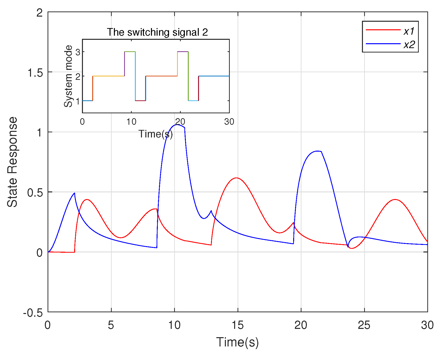
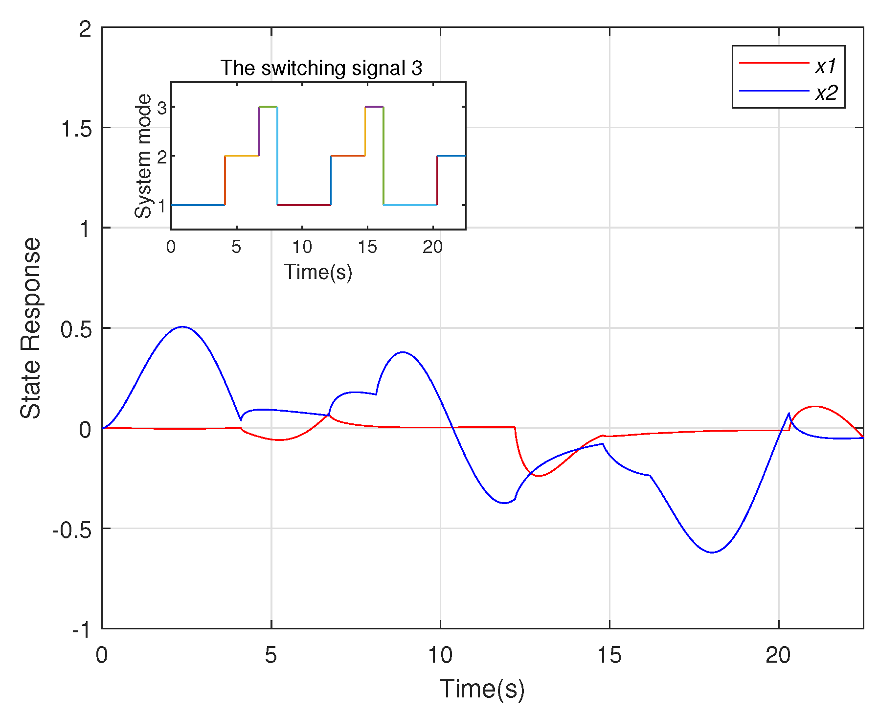
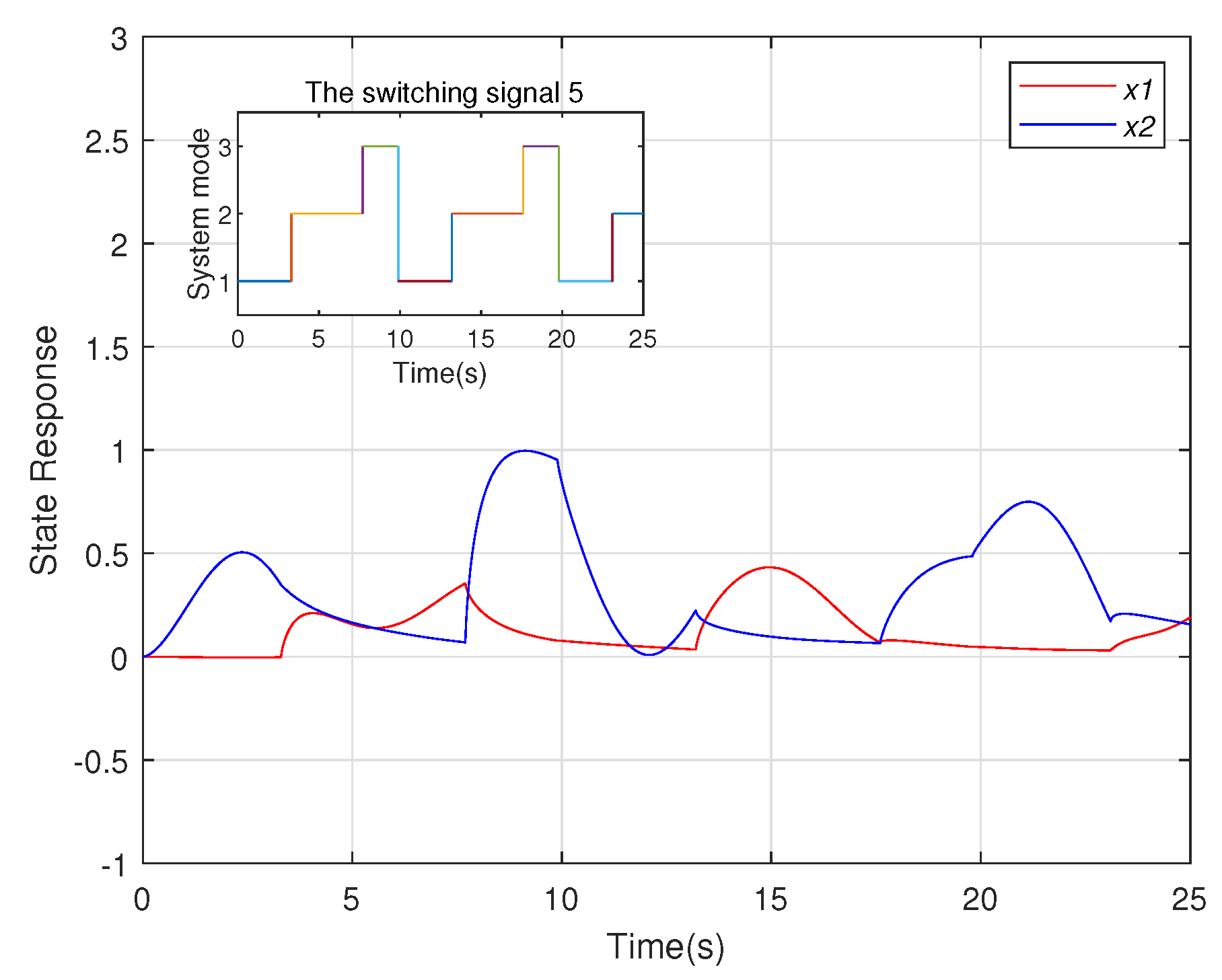
4. Numerical Example

In this section, a numerical example in the continuous-time domain will be provided to verify the effectiveness of the theoretical results.

Example

Consider electrical circuits consisting of superconductors, resistors, resistor, coils, and current voltage sources. In practical problems, the circuit always contains external perturbation signals such as environment, human factors, and circuit aging. By using Kirchhoff’s laws and the relations (2.82), (2.83) in [34], the switching-type fractional linear circuit system can be written as system (3). Here, x 1 ( s ) R n 1 is voltage between the superconductors, x 2 ( s ) R n 2 is the current in the coil and u ( s ) R m is the voltage of the circuit. Then, consider switched linear system (3) ( u = 0 ) , and the parameters given as follows:
A 1 = 0.3 0 0.8 0.2 , A 2 = 0.3 1 0 0.25 , A 3 = 0.4 0 3 0.2 ,
B 1 = 0.27 0 30 0.2875 , B 2 = 0.5 16.43 0 0.35 , B 3 = 0.3 0 1.3 0.375 ,
D ¯ 1 = 1.6 0 0 1.8 , D ¯ 3 = 1.4 0 0 1.6 ,
E 1 = E 2 = E 3 = 1 0 0 1 ,
Π 1 = Π 2 = Π 3 = 1 0 0 0 .
It is easy to show that all subsystems are regular and impulse-free by employing Lemma 6. To verify the comprehensiveness of the presented results, we make a few comparisons by the ADT, MDADT, and ΦDADT switching approach.
Let β = 0.75 , F = 1 , Q = 1 and S γ = S p = S h = 15 . If we take the disturbance input ω ( s ) = 0.01 sin s , then we can choose d = 0.0001 to guarantee that ω T ( s ) F ω ( s ) d , s [ 0 , 15 ] .
Table 1 presents the following facts by choosing a different ( Φ , O ) .
(I) For different Φ , the ΦDADT method provides the different results of admissible signals with their own merits. Let O = { 1 , 2 } , for case (i): Φ 1 = { 1 , 2 } , Φ 2 = { 3 } , the 1st and 2nd modes having ADT 2.1304 and the 3rd mode with ADT 4.3066 ; for case (ii): Φ 1 = { 1 , 3 } , Φ 2 = { 2 } , the 1st and 3rd modes having ADT 2.7429 , and the 2nd mode with ADT 2.5783 ; for case (iii): Φ 1 = { 2 , 3 } , Φ 2 = { 1 } , the 2nd and 3rd modes with ADT 3.6560 , and the 1st mode having ADT 1.5372 . (iv): Φ 1 = { 1 , 2 , 3 } , the 1st, 2nd and 3rd modes with ADT 3.2443 ; (v): Φ 1 = { 1 } , Φ 2 = { 2 } , Φ 3 = { 3 } the 1st mode with ADT 3.2443 , the 2nd mode with ADT 4.3066 and 3rd mode with ADT 2.1304 .
(II) A fact can be presented from Table 1, each column has its own characteristics by choosing a different ( Φ , O ) . Therefore, we cannot decide which is better.
(III) When O = { 1 } , we take μ = 3 , and λ = 0.3 . By solving the conditions in our Theorem 1 and Theorem 1 in [26], we can obtain τ a Φ * = 3.2443 and τ a * = 5.2976 . The ADT has a smaller value of τ a Φ * than the ADT value τ a * in [26]. Therefore, the new result has a larger feasible region than the result in that work.
Figure 1, Figure 2, Figure 3, Figure 4 and Figure 5 show the simulation results of the system with x 0 = [ 0 , 0 ] T under the corresponding switching signals. State trajectories of system (3) with the ADT (signal 1) and MDADT (signal 5) are shown in Figure 1 and Figure 5, respectively. State trajectories of system (3) under ΦDADT with O = { 1 , 2 } (signals 2, 3 and 4) are depicted in Figure 2, Figure 3 and Figure 4, respectively.

5. Conclusions

This paper studied the problem of FTS for FOSSS with D-perturbation. By using the ΦDADT approach and constructing the multiple Lyapunov functions, an output feedback controller was designed. Then, some sufficient conditions were derived for the considered systems to ensure their IO-FTS by linear matrix inequalities. Finally, a numerical example illustrates the superiority of the proposed method. In further work, we will extend the proposed method to FOSSS with time delays.

Author Contributions

Conceptualization, Q.Y.; Methodology, Q.Y.; Validation, N.X.; Formal analysis, Q.Y.; Investigation, Q.Y. and N.X.; Writing—original draft, Q.Y. and N.X.; Writing—review & editing, Q.Y.; Visualization, N.X.; Project administration, Q.Y.; Funding acquisition, Q.Y. All authors have read and agreed to the published version of the manuscript.

Funding

Supported by Fundamental Research Program of Shanxi Province (202103021224249) and Fund Program for the Scientific Activities of Selected Returned Overseas Professionals in Shanxi Province (20220023).

Data Availability Statement

The data supporting reported results are available from the corresponding author upon reasonable request.

Conflicts of Interest

The authors declare no conflict of interest.

Nomenclature

ADTaverage dwell time
MDADTmode-dependent average dwell time
ΦDADTΦ-dependent average dwell time
FOSSSfractional-order switched singular systems
FOPSSfractional-order positive switched systems
FOMSfractional-order multiagent systems
LMIslinear matrix inequalities
FTSfinite-time stability
FTBfinite-time boundedness
IO-FTSinput-output finite-time stability

References

  1. Montseny, G.; Audounet, J.; Mbodje, B. Optimal models of fractional integrators and application to systems with fading memory. In Proceedings of the IEEE Systems Man and Cybernetics Conference—SMC, Le Touquet, France, 17–20 October 1993; Volume 5, pp. 65–70. [Google Scholar]
  2. Suki, B.; Barabasi, A.L.; Lutchen, K.R. Lung tissue viscoelasticity: A mathematical framework and its molecular basis. J. Appl. Physiol. 1994, 76, 2749–2759. [Google Scholar] [CrossRef] [PubMed]
  3. Heleschewitz, Z.; Matignon, D. Diffusive realisations of fractional integrodifferential operators: Structural analysis under approximation. IFAC Proceedings Volumes 1998, 31, 227–232. [Google Scholar] [CrossRef]
  4. Yang, X.J.; Baleanu, D. Fractal heat conduction problem solved by local fractional variation iteration. Therm. Sci. 2013, 17, 625–628. [Google Scholar] [CrossRef]
  5. Yin, C.; Huang, X.; Chen, Y.; Dadras, S.; Zhong, S.-M.; Cheng, Y. Fractional-order exponential switching technique to enhance sliding mode control. Appl. Math. Model. 2017, 44, 705–726. [Google Scholar] [CrossRef]
  6. Yin, C.; Huang, X.; Dadras, S.; Cheng, Y.; Cao, J.; Malek, H.; Mei, J. Design of optimal lighting control strategy based on multi-variable fractional-order extremun seeking method. Inf. Sci. 2018, 465, 38–60. [Google Scholar] [CrossRef]
  7. Owolabi, K.M.; Gómez-Aguilar, J.; Karaagac, B. Modelling analysis and simulations of some chaotic systems using derivative with Mittag-Leffler kernel. Chaos Solutions Fractals 2019, 125, 54–63. [Google Scholar] [CrossRef]
  8. Babiarz, A.; Legowski, A.; Niezabitowski, M. Controllability of positive discrete-time switched fractional order systems for fixed switching sequence. In Proceedings of the 8th International Conference, ICCCI 2016, Halkidiki, Greece, 28–30 September 2016. [Google Scholar]
  9. Zhao, X.D.; Yin, Y.F.; Zheng, X.L. State-dependent switching control of switched positive fractional-order systems. ISA Trans. 2016, 62, 103–108. [Google Scholar] [CrossRef]
  10. Dadras, S.; Malek, H.; Chen, Y. A note on the Lyapunov stability of fractional-order nonlinear systems. In Proceedings of the ASME 2017 International Design Engineering Technical Conferences & Computers and Information in Engineering Conference, Cleveland, OH, USA, 6–9 August 2017; American Society of Mechanical Engineers: New York, NY, USA, 2017. [Google Scholar]
  11. Thuan, M.V.; Huong, D.C. New results on stabilization of fractional-order nonlinear systems via an LMI approach. Asian J. Control 2018, 20, 1541–1550. [Google Scholar] [CrossRef]
  12. Zhang, J.F.; Zhao, X.D.; Chen, Y. Finite-time stability and stabilization of fractional order positive switched systems. Circuits Syst. Singal Process. 2016, 35, 2450–2470. [Google Scholar] [CrossRef]
  13. Yang, Y.; Chen, G. Finite-time stability of fractional order impulsive switched systems. Int. J. Robust Nonlinear Control. 2015, 25, 2207–2222. [Google Scholar] [CrossRef]
  14. Liu, L.P.; Cao, X.Y.; Fu, Z.M.; Song, S.Z.; Xing, H. Finite-time control of uncertain fractional-order positive impulsive switched systems with mode-dependent average dwell time. Circuits Syst. Signal Process. 2018, 37, 3739–3755. [Google Scholar] [CrossRef]
  15. Liu, L.P.; Cao, X.Y.; Fu, Z.M.; Song, S.Z.; Xing, H. Positive impulsive observer design of fractional-order positive switched systems with MDADT. Trans. Inst. Meas. Control 2019, 41, 1340–1347. [Google Scholar] [CrossRef]
  16. Liang, J.X.; Wu, B.W.; Liu, L.L.; Wang, Y.E.; Li, C.T. Finite-time stability and finite-time boundedness of fractional order switched systems. Trans. Inst. Meas. Control 2019, 41, 3364–3371. [Google Scholar] [CrossRef]
  17. Chen, Y.; Wen, G.; Peng, Z.; Rahmani, A. Consensus of fractional-order multi-agent system via sampled-data event-triggered control. J. Frankl. Institue 2019, 356, 10241–10259. [Google Scholar] [CrossRef]
  18. Hu, T.; He, Z.; Zhang, X. Leader-following consensus of fractional-order multi-agent systems based on event-triggered control. Nonlinear Dyn. 2020, 99, 2219–2232. [Google Scholar] [CrossRef]
  19. Feng, T.; Guo, L.H.; Wu, B.W.; Chen, Y.Q. Stability analysis of switched fractional-order continuous-time systems. Nonlinear Dyn. 2020, 102, 2467–2478. [Google Scholar] [CrossRef]
  20. Zong, G.D.; Wang, X.H.; Zhao, H.J. Robust finite-time guaranteed cost control for impulsive switched systems with time-varying delay. Int. J. Control Autom. Syst. 2017, 15, 113–121. [Google Scholar] [CrossRef]
  21. Shang, Y.L.; Liu, L.P.; Di, Y.F.; Fu, Z.M.; Fan, B.O. Guaranteed cost and finite-time event-triggered control of fractional-order switched systems. Trans. Inst. Measrement Control 2021, 43, 2724–2733. [Google Scholar] [CrossRef]
  22. Liu, L.P.; Di, Y.F.; Shang, Y.L.; Fu, Z.M.; Fan, B. Guaranteed Cost and Finite-Time Non-fragile Control of Fractional-Order Positive Switched Systems with Asynchronous Switching and Impulsive Moments. Circuits Syst. Signal Process. 2021, 40, 3143–3160. [Google Scholar] [CrossRef]
  23. Yu, Q.; Zhai, G.S. Stability analysis of switched systems under Φ-dependent average dwell time. IEEE Access. 2020, 8, 30655–30663. [Google Scholar] [CrossRef]
  24. Thanh, N.T.; Phat, V.N. Switching law design for finite-time stability of singular fractional-order systems with delay. IET Control Theory Appl. 2018, 13, 1367–1373. [Google Scholar] [CrossRef]
  25. Wang, Z.; Ding, Y.X.; Pan, F. Observer-based robust control for singular switched fractional order systems subject to actuator saturation. Appl. Math. Comput. 2021, 411, 126538. [Google Scholar] [CrossRef]
  26. Feng, T.; Wu, B.W.; Wang, Y.-E.; Liu, L.L. Input-output finite-time stability of fractional-order switched singular continuous-time systems. Asian J. Control. Affil. Acpa. Asian Control. Profr. Assoc. 2019, 23, 1052–1061. [Google Scholar] [CrossRef]
  27. Liu, J.; Lian, J.; Zhuang, Y. Robust stability for switched positive systems with D-perturbation and time-varying delay. Inf. Sci. 2016, 369, 522–531. [Google Scholar] [CrossRef]
  28. Xing, H.; Liu, L.P.; Cao, X.Y.; Fu, Z.M.; Song, S.Z. Guaranteed cost finite-time control of positive switched nonlinear systems with D-perturbation. Nephron Clin. Pract. 2017, 15, 1635–1648. [Google Scholar] [CrossRef]
  29. Liu, L.P.; Cao, X.Y.; Fu, Z.M.; Song, S.Z. Guaranteed cost finite-time control of fractional-order nonlinear positive switched systems with D-Perturbations via MDADT. J. Syst. Sci. Complex. 2019, 32, 857–874. [Google Scholar] [CrossRef]
  30. Delavari, H.; Baleavanu, D.; Sadati, J. Stability analysis of Caputo fractional-order nonlinear systems. Nonlinear Dyn. 2012, 67, 2433–2439. [Google Scholar] [CrossRef]
  31. N’Doye, I.; Darouach, M.; Zasadzinski, M.; Radhy, N.E. Robust stabilization of uncertain descriptor fractional-order systems. Automatica 2013, 49, 1907–1913. [Google Scholar] [CrossRef]
  32. Zhang, X.F.; Chen, Y.C. Admissibility and robust stabilization of continuous linear singular fractional order systems with the fractional order α: The 0 < α < 1 case. ISA Trans. 2018, 82, 42–50. [Google Scholar] [PubMed]
  33. Zhou, L.; Ho, D.W.C.; Zhai, G. Stability analysis of switched linear singular systems. Automaica 2013, 49, 1481–1487. [Google Scholar] [CrossRef]
  34. Kaczorek, T. Selected Problems of Fractional Systems Theory; Springer: Berlin/Heidelberg, Germany, 2012; pp. 48–54. [Google Scholar]
Figure 1. The state response of the system under the signal 1.
Fractalfract 07 00341 g001
Figure 2. The state response of the system under the signal 2.
Fractalfract 07 00341 g002
Figure 3. The state response of the system under the signal 3.
Fractalfract 07 00341 g003
Figure 4. The state response of the system under the signal 4.
Fractalfract 07 00341 g004
Figure 5. The stateresponse of the system under the signal 5.
Fractalfract 07 00341 g005
Table 1. Comparison of the results under three switching approaches ( x 0 = [ 0 , 0 ] T ).
O ADT { 1 } { 1 , 2 } MDADT { 1 , 2 , 3 }
Φ i Φ 1 = { 1 , 2 , 3 } Φ 1 = { 1 , 2 } Φ 1 = { 1 , 3 } Φ 2 = { 2 , 3 } Φ 1 = { 1 }
Φ 2 = { 3 } Φ 2 = { 2 } Φ 1 = { 1 } Φ 2 = { 2 }
Φ 3 = { 3 }
μ μ 1 = 3 μ 1 = 2 μ 1 = 2.5 μ 1 = 2 μ 1 = 3 , μ 2 = 3
μ 2 = 3 μ 2 = 3 μ 2 = 2.5 μ 3 = 2
λ λ = 0.3 λ 1 = 0.3 λ 1 = 0.3 λ 1 = 0.2 λ 1 = 0.3 , λ 2 = 0.4
λ 2 = 0.4 λ 2 = 0.2 λ 2 = 0.4 λ 3 = 0.3
P 1 0.0201 0.0003 🟉 0.0000 0.0127 0.0003 🟉 0.0001 0.0729 0.0004 🟉 0.0001 0.0664 0.0004 🟉 0.0001 0.1489 0.0010 🟉 0.0001
P 2 0.0000 0.0003 🟉 0.0062 0.0001 0.0007 🟉 0.0060 0.0003 0.0009 🟉 0.0617 0.0004 0.0010 🟉 0.0732 0.0006 0.0023 🟉 0.1385
P 3 0.0089 0.0450 🟉 0.0041 0.0018 0.0274 🟉 0.0062 0.0108 0.0656 🟉 0.0165 0.0131 0.0693 🟉 0.0128 0.0257 0.1128 🟉 0.0413
Signal design τ a Φ 1 * = 3.2443 τ a Φ 1 * = 2.1304 τ a Φ 1 * = 2.7429 τ a Φ 1 * = 1.5327 τ a Φ 1 * = 3.2443
τ a Φ 2 * = 4.3066 τ a Φ 2 * = 2.5783 τ a Φ 2 * = 3.6560 τ a Φ 2 * = 4.3066
τ a Φ 3 * = 2.1304
Signal instance τ 1 = 6.5 , τ 2 = 2.1 τ 1 = 2.1 , τ 2 = 6.5 τ 1 = 4.1 , τ 2 = 2.6 τ 1 = 1.6 , τ 2 = 5.2 τ 1 = 3.3 , τ 2 = 4.4
τ 3 = 1.2 τ 3 = 2.2 τ 3 = 1.4 τ 3 = 2.1 τ 3 = 2.2
State response under
signal instance
Figure 1Figure 2Figure 3Figure 4Figure 5
Disclaimer/Publisher’s Note: The statements, opinions and data contained in all publications are solely those of the individual author(s) and contributor(s) and not of MDPI and/or the editor(s). MDPI and/or the editor(s) disclaim responsibility for any injury to people or property resulting from any ideas, methods, instructions or products referred to in the content.

