Compact Difference Schemes with Temporal Uniform/Non-Uniform Meshes for Time-Fractional Black–Scholes Equation

Abstract

In this paper, we are interested in the effective numerical schemes of the time-fractional Black–Scholes equation. We convert the original equation into an equivalent integral-differential equation and then discretize the time-integral term in the equivalent form using the piecewise linear interpolation, while the compact difference formula is applied in the spatial direction. Thus, we derive a fully discrete compact difference scheme with second-order accuracy in time and fourth-order accuracy in space. Rigorous proofs of the corresponding stability and convergence are given. Furthermore, in order to deal effectively with the non-smooth solution, we extend the obtained results to the case of temporal non-uniform meshes and obtain a temporal non-uniform mesh-based compact difference scheme as well as the numerical theory. Finally, extensive numerical examples are included to demonstrate the effectiveness of the proposed compact difference schemes.

1. Introduction

In this paper, we are interested in the effective numerical schemes for the following time-fractional Black–Scholes (B-S) equation governing European options [1]:

$$\frac{{\partial }^{\alpha }V}{\partial t^{\alpha }}+\frac{1}{2}{\sigma }^2{S}^2\frac{{\partial }^{2}V}{\partial S^2}+(r-D)S\frac{\partial V}{\partial S}-rV=0,$$

(1)

with the boundary conditions $V(S_l,t)=P(t),V(S_r,t)=Q(t),t\in (0,T)$ and terminal condition $V(S,T)=H(S),S\in (S_l,S_r)\subset {\mathbb{R}}^{+}$. Here, $V(S,t)$ denotes the price of a European-style double-barrier option with S being the asset price and t being the current time. The parameter $\sigma$ is the volatility of the returns, r is the risk-free interest rate, and D is the dividend rate. The fractional operator $\frac{{\partial }^{\alpha }}{\partial t^{\alpha }}$ with the fractional order $\alpha \in (0,1)$ is defined by

$$\frac{{\partial }^{\alpha }V}{\partial t^{\alpha }}=\frac{1}{\Gamma (1-\alpha )}\frac{\partial }{\partial t}{\int }_t^T{(\varkappa -t)}^{-\alpha }(V(S,\varkappa )-V(S,T))d\varkappa .$$

The functions P and Q in the boundary condition are the rebates paid when the corresponding barrier is hit and the function H in the terminal condition is the payoff function.

The time-fractional B-S model (1) is derived by assuming that the change in the option price with time is a fractal transmission system. Some scholars have made some achievements in the study of this model or related field; see [1,2,3,4], just to name a few.

Since the analytical solution of the time-fractional B-S model (1) is difficult to obtain, we need to resort to numerical methods to better investigate the dynamical behavior of this model. Some efforts on the study of numerical methods have been made so far; see [5,6,7] and the references therein. In [5], Zhang et al. constructed a discrete implicit difference scheme with accuracy of $O({\tau }^{2-\alpha }+h^2)$, where $\tau$ and h are the temporal step size and spatial step size, respectively. Later on, De Staelen and Hendy improved Zhang et al.’s results by proposing a finite difference scheme of spatial fourth-order accuracy while keeping temporal $2-\alpha$ order accuracy [6]. Different from the above mentioned central difference method or compact difference method for discretization in space, Roul utilized the collocation method based on quintic B-spline basis functions for spatial discretization and the backward Euler method for temporal discretiztion [7]. The resulting numerical scheme was shown to be stable with accuracy of $O({\tau }^{2-\alpha }+h^4)$.

It is noted that both theoretical and numerical tests of the above mentioned numerical schemes are discussed under the solution of the time-fractional B-S equation is sufficiently smooth. Generally speaking, the solution of the time-fractional model (1) has weak singularity near $t=0$ due to the non-smooth payoff function, which would have certain impact on the accuracy of the derived numerical scheme. This is already a common fact in the fractional community; see the two review papers [8,9] or the book [10] for more discussion of the related topic. One of the most common and effective ways of dealing with the insufficiently smooth solution of time-fractional models is the use of non-uniform meshes; e.g., see [11,12,13,14].

In [15], Cen et al. transformed the time-fractional B-S equation into an equivalent integral-differential equation and proposed a finite difference scheme on a temporal adapted mesh. Although the proposed temporal non-uniform meshes-based finite difference scheme takes into account the possible singularity behavior of the analytic solution near $t=0$, it has only first-order and second-order accuracy in time and in space, respectively. Similarly, based on the equivalent integral differential equation, Kazmi developed a finite difference scheme with second-order accuracy in both space and time [16]. The author obtained asymptotic error expansions for numerical solutions of non-smooth problems based on the observation of numerical results and employed the Richardson extrapolation technique to improve the accuracy of the numerical scheme. In [17], Song and Lyu constructed an efficient finite difference scheme by employing the non-uniform Alikhanov formula. It can be seen that there is some room for improvement in the efficient numerical scheme for time-fractional B-S equation, especially for non-smooth solution problems.

Motivated by the ideas in Li et al. [11], we develop the efficient finite difference schemes with temporal uniform/non-uniform meshes for solving the time-fractional B-S Equation (1). More precisely, we first transform the original equation into an equivalent integral-differential equation with a weakly singular kernel and then use the piecewise linear interpolation function to discretize the time integral terms in the equivalent form and use the compact difference method to discretize the spatial direction. Thus, we finally obtain the fully discrete compact difference schemes.

The main contributions of this paper are listed as follows: First, we propose the compact difference schemes with temporal uniform/non-uniform meshes. The derived schemes handle well the effect of the non-smooth payoff function in (1) and can be easily implemented on the computer. Second, based on Fourier analysis, we provide rigorous proofs of the stability and convergence of the uniform meshes-based compact difference scheme and extend to the theoretical analysis of the temporal non-uniform mesh-based compact difference scheme. Third, we present extensive numerical tests, including comparisons with other existing finite difference schemes, particularly the two schemes presented in [16,18], for smooth/non-smooth solution problems to illustrate the advantages of our schemes.

The rest of the paper is organized as follows. The uniform mesh-based compact difference scheme is derived in the next section. Stability and error estimate of the derived numerical scheme are provided in Section 3. In Section 4, we extend the results based on the uniform meshes to the non-uniform mesh case and derive the temporal non-uniform mesh-based compact difference scheme and give the corresponding numerical theoretical results. In Section 5, extensive numerical examples are presented to demonstrate the performance of the derived schemes. Finally, the conclusions are given in Section 6.

2. The Derivation of the Scheme

For the convenience of numerical solution, we transform the original Equation (1) into another equivalent form with the help of variable substitution. That is, we set $\varsigma =T-t$ and denote $x=lnS$ and $u(x,\varsigma )=V(S,t)$. After some routine calculations for (1), one can obtain

$$\begin{array}{ccc}\hfill \frac{{\partial }^{\alpha }V}{\partial t^{\alpha }}& =& -{}_C{D}_{0,\varsigma }^{\alpha }u,\hfill \\ \hfill \frac{\partial V}{\partial S}& =& e^{-x}\frac{\partial u}{\partial x},\hfill \\ \hfill \frac{{\partial }^{2}V}{\partial S^2}& =& e^{-2x}\left(\frac{{\partial }^{2}u}{\partial x^2}-\frac{\partial u}{\partial x}\right),\hfill \end{array}$$

which leads to the following equivalent form:

$${}_C{D}_{0,\varsigma }^{\alpha }u(x,\varsigma )=p\frac{{\partial }^{2}u(x,\varsigma )}{\partial x^2}+q\frac{\partial u(x,\varsigma )}{\partial x}-ru(x,\varsigma ),(x,\varsigma )\in (x_l,x_r)\times (0,T].$$

Here, $p=\frac{{\sigma }^2}{2}$ and $q=r-D-p$. The Caputo derivative ${}_C{D}_{0,\varsigma }^{\alpha }u(x,\varsigma )$ is defined by

$${}_C{D}_{0,\varsigma }^{\alpha }u(x,\varsigma )=\frac{1}{\Gamma (1-\alpha )}{\int }_0^{\varsigma }{(\varsigma -s)}^{-\alpha }\frac{\partial u(x,s)}{\partial s}ds.$$

Thus, without loss of generality, we consider the following time-fractional problem:

$${}_C{D}_{0,t}^{\alpha }u(x,t)={\mathcal{L}}_{x}u(x,t)+f(x,t),(x,t)\in (x_l,x_r)\times (0,T],$$

(2)

with the boundary conditions $u(x_l,t)=\phi (t),u(x_r,t)=\nu (t),t\in [0,T]$, and the initial condition $u(x,0)=h(x),x\in [x_l,x_r]$. Here, $f(x,t)$ is a suitable smooth function and

$${\mathcal{L}}_{x}u(x,t)=p\frac{{\partial }^{2}u(x,t)}{\partial x^2}+q\frac{\partial u(x,t)}{\partial x}-ru(x,t).$$

(3)

Remark 1. 

It is worth noting that the forms of the functions $\phi ,\nu$, and h in the boundary and initial conditions of (2) will vary depending on the pricing model. For example, for the European put option, we let $\phi (t)=K{e}^{-rt},\nu (t)=0$ and $h(x)=max\{K(1-e^x),0\}$, with K being the strike price of the option. One may refer to [16] or [1] for more discussions.

We first introduce some useful notations. For positive integers $M_x$ and $N_t$, let the spatial step size and temporal step size be $h=(x_r-x_l)/M_x$ and $\tau =T/N_t$, respectively. The discrete grids in space are given by ${\overline{\Omega }}_h=\left\{x_m\right|0\le m\le M_x\}$ with the grid points $x_m=x_l+mh,m=0,1,2,\cdots ,M_x$. Let the grid points in time be $t_n=n\tau ,n=0,1,2,\cdots ,N_t$. Let $v=\{v_i=v(x_i)|0\le i\le M_x\}$ be a grid function defined on ${\overline{\Omega }}_h$. We define spatial difference operators ${\delta }_x^2{v}_i=\frac{v_{i+1}-2v_i+v_{i-1}}{h^2}$ and ${\delta }_{\widehat{x}}{v}_i=\frac{v_{i+1}-v_{i-1}}{2h}$.

It is known that the Equation (2) is equivalent to the Volterra integro-differential equation:

$$u(x,t)=u(x,0)+\frac{1}{\Gamma (\alpha )}{\int }_0^t{(t-s)}^{\alpha -1}({\mathcal{L}}_{x}u(x,s)+f(x,s))ds.$$

(4)

Considering the above Equation (4) at the grid point $(x_m,t_n)$, we have

$$u_m^n=u_m^0+\frac{1}{\Gamma (\alpha )}\sum _{j=0}^{n-1}{\int }_{t_j}^{t_{j+1}}{(t_n-s)}^{\alpha -1}g(s)ds,$$

(5)

where $u_m^n=u(x_m,t_n)$ and $g(s):={\mathcal{L}}_{x}u(x_m,s)+f(x_m,s)$.

Suppose that $g(s)\in C^2[0,T]$. Applying the piecewise linear interpolation on each sub-interval $[t_j,t_{j+1}]$ to approximate the integrand $g(s)$, one has

$$g(s)\approx \frac{t_{j+1}-s}{\tau }g(t_j)+\frac{s-t_j}{\tau }g(t_{j+1}),0\le j\le n-1.$$

So, it follows from (5) that

$$u_m^n=u_m^0+\sum _{j=0}^n{w}_{n-j}^{(n)}({\mathcal{L}}_{x}u(x_m,t_j)+f(x_m,t_j))+r_m^n,$$

(6)

where the weights are given by

$$\begin{array}{c}\hfill w_j^{(n)}=\mu \left\{\begin{array}{cc}& {(n-1)}^{\alpha +1}-(n-1-\alpha )n^{\alpha },j=n\hfill \\ & {(j+1)}^{\alpha +1}-2j^{\alpha +1}+{(j-1)}^{\alpha +1},1\le j\le n-1,\hfill \\ & 1,j=0,\hfill \end{array}\right.\end{array}$$

(7)

with $\mu =\frac{{\tau }^{\alpha }}{\Gamma (\alpha +2)}$, and the truncation error term $r_m^n=O({\tau }^2)$.

Next, we consider the compact difference method to obtain the fully discrete numerical scheme for (6). To this end, we begin with the compact difference method for the following steady state equation:

$$p\frac{d^{2}u(x)}{d{x}^2}+q\frac{du(x)}{dx}-ru(x)=v(x),$$

(8)

where $v(x)$ is a suitable smooth function.

Utilizing the Taylor expansion, one can derive the fourth-order compact finite difference scheme to solve Equation (8) (see Theorem 1 in [18]), that is,

$${\mathcal{H}}_{1}u(x_m)={\mathcal{H}}_{2}v(x_m)+O(h^4),$$

(9)

where

$$\begin{array}{ccc}\hfill {\mathcal{H}}_1& =& (p-\frac{h^2}{12}(r-\frac{q^2}{p})){\delta }_x^2+(q-\frac{h^2}{12}\frac{qr}{p}){\delta }_{\widehat{x}}-r,\hfill \\ \hfill {\mathcal{H}}_2& =& 1+\frac{h^2}{12}{\delta }_x^2+\frac{q}{p}\frac{h^2}{12}{\delta }_{\widehat{x}}.\hfill \end{array}$$

Noting the definition of ${\mathcal{L}}_x$ in (6) and so combining Equations (6) and (9), one obtains

$$\begin{array}{ccc}\hfill {\mathcal{H}}_{2}u(x_m,t_n)& =& {\mathcal{H}}_{2}u(x_m,0)+\sum _{j=0}^n{w}_{n-j}^{(n)}{\mathcal{H}}_{1}u(x_m,t_j)\hfill \\ & & +\sum _{j=0}^n{w}_{n-j}^{(n)}{\mathcal{H}}_{2}f(x_m,t_j)+R_m^n,\hfill \end{array}$$

(10)

where $R_m^n=O({\tau }^2+h^4)$. Dropping the small term $R_m^n$, and replacing $u_m^n$ with the approximate solution $U_m^n$, we obtain the following fully discrete compact difference scheme:

$${\mathcal{H}}_2{U}_m^n={\mathcal{H}}_2{U}_m^0+\sum _{j=0}^n{w}_{n-j}^{(n)}{\mathcal{H}}_1{U}_m^j+\sum _{j=0}^n{w}_{n-j}^{(n)}{\mathcal{H}}_2{f}_m^j,$$

(11)

with $m=1,2,\cdots ,M_x-1$ and $n=1,2,\cdots ,N_t$. The corresponding initial and boundary conditions are given by $U_j^0=h(x_j),j=0,1,\cdots ,M_x,$ and $U_0^n=\phi (t_n),U_{M_x}^n=\nu (t_n),n=1,2,\cdots ,N_t.$

To facilitate code implementation and theoretical analysis, we expand on the original compact difference scheme (11) below. Observing that the $U_m^n$ on the right-hand side of (11) is unknown, moving it to the left-hand side and using the definitions of ${\mathcal{H}}_j(j=1,2)$, we obtain

$$\begin{array}{ccc}& & U_m^n+\frac{q}{p}\frac{h^2}{12}\frac{U_{m+1}^n-U_{m-1}^n}{2h}+\frac{h^2}{12}\frac{U_{m-1}^n-2U_m^n+U_{m+1}^n}{h^2}\hfill \\ & & -\mu (p-\frac{h^2}{12}(q-\frac{q^2}{p}))\frac{U_{m-1}^n-2U_m^n+U_{m+1}^n}{h^2}\hfill \\ & & -\mu \left((q-\frac{h^2}{12}\frac{qr}{p})\frac{U_{m+1}^n-U_{m-1}^n}{2h}-r{U}_m^n\right)\hfill \\ & =& \sum _{j=0}^{n-1}{w}_{n-j}^{(n)}[(p-\frac{h^2}{12}(r-\frac{q^2}{p}))\frac{U_{m-1}^j-2U_m^j+U_{m+1}^j}{h^2}\hfill \\ & & +(q-\frac{h^2}{12}\frac{qr}{p})\frac{U_{m+1}^j-U_{m-1}^j}{2h}-r{U}_m^j]\hfill \\ & & +U_m^0+\frac{q}{p}\frac{h^2}{12}\frac{U_{m+1}^0-U_{m-1}^0}{2h}+\frac{h^2}{12}\frac{U_{m-1}^0-2U_m^0+U_{m+1}^0}{h^2}\hfill \\ & & +\sum _{j=0}^n{w}_{n-j}^{(n)}\left[f_m^j+\frac{h^2}{12}\frac{f_{m-1}^j-2f_m^j+f_{m+1}^j}{h^2}+\frac{q}{p}\frac{h^2}{12}\frac{f_{m+1}^j-f_{m-1}^j}{2h}\right].\hfill \end{array}$$

To simplify the above equation, we set

$$a=\frac{q}{p}h,b=\frac{p-\frac{h^2}{12}(r-\frac{q^2}{p})}{h^2},c=\frac{q-\frac{h^2}{12}\frac{qr}{p}}{2h}.$$

(12)

Thus, after some trivial operations, we obtain

$$\begin{array}{ccc}\hfill & & (-\frac{a}{24}+\frac{1}{12}-\mu b+\mu c)U_{m-1}^n+(\frac{5}{6}+2\mu b+\mu r)U_m^n+(\frac{a}{24}+\frac{1}{12}-\mu b-\mu c)U_{m+1}^n\hfill \\ & =& (-\frac{a}{24}+\frac{1}{12})U_{m-1}^0+\frac{5}{6}{U}_m^0+(\frac{a}{24}+\frac{1}{12})U_{m+1}^0\hfill \\ & & +\sum _{j=0}^{n-1}{w}_{n-j}^{(n)}\left[(b-c)U_{m-1}^j+(-2b-r)U_m^j+(b+c)U_{m+1}^j)\right]\hfill \\ & & +\sum _{j=0}^n{w}_{n-j}^{(n)}\left[(-\frac{a}{24}+\frac{1}{12})f_{m-1}^j+\frac{5}{6}{f}_m^j+(\frac{a}{24}+\frac{1}{12})f_{m+1}^j\right].\hfill \end{array}$$

(13)

The above equations can be written in a more compact matrix-vector form. Denoted by ${\mathbf{u}}^n={(U_1^n,U_2^n,\cdots ,U_{M_x-1}^n)}^T$ and ${\mathbf{f}}^n={(f_1^n,f_2^n,\cdots ,f_{M_x-1}^n)}^T$, one has the following matrix form for (13):

$$\mathbf{A}{\mathbf{u}}^n={\mathbf{F}}^n,$$

where ${\mathbf{F}}^n=\mathbf{D}{\mathbf{u}}^0+\mathbf{E}{\sum }_{j=0}^{n-1}{w}_{n-j}^{(n)}{\mathbf{u}}^j+\mathbf{D}{\sum }_{j=0}^n{w}_{n-j}^{(n)}{\mathbf{f}}^j+{\mathbf{q}}^n$. The matrices $\mathbf{A}$, $\mathbf{D}$, and $\mathbf{E}$ are all $(M_x-1)\times (M_x-1)$ tridiagonal matrices given by $\mathbf{A}=\mathbf{D}-\mu \mathbf{E}$ with

$$\mathbf{D}=diag(-\frac{a}{24}+\frac{1}{12},\frac{5}{6},\frac{a}{24}+\frac{1}{12})$$

and $\mathbf{E}=diag(b-c,-2b-r,b+c)$. The column vector ${\mathbf{q}}^n$ with $(M_x-1)$ entries is defined by

$$\begin{array}{ccc}\hfill {\mathbf{q}}^n& =& [(-\frac{a}{24}+\frac{1}{12})(U_0^0-U_0^n)+\sum _{j=0}^n{w}_{n-j}^{(n)}[(b-c)\phi (t_j)+(-\frac{a}{24}+\frac{1}{12})f_0^j],\hfill \\ & & 0,\cdots ,0,\hfill \\ & & (\frac{a}{24}+\frac{1}{12})(U_{M_x}^0-U_{M_x}^n)+\sum _{j=0}^n{w}_{n-j}^{(n)}[(b+c)\nu (t_j)+(\frac{a}{24}+\frac{1}{12})f_{M_x}^j]{]}^T.\hfill \end{array}$$

It can be readily seen that the compact difference scheme (13) is uniquely solvable. Indeed, by the definitions of the parameters $\mu ,a,b,c,$ and r, one can observe that the inequality

$$|\frac{5}{6}+2\mu b+\mu r|>|-\frac{a}{24}+\frac{1}{12}-\mu b+\mu c|+|\frac{a}{24}+\frac{1}{12}-\mu b-\mu c|$$

holds when $\tau$ and h are both small. This implies that the coefficient matrix $\mathbf{A}$ in the matrix form of (13) is strictly diagonally dominant and thus it is non-singular. Therefore, the unique solvability of (13) follows.

3. Stability and Error Estimate

In this section, the stability and error estimate of the proposed compact difference scheme (11) are discussed by the method of Fourier analysis.

3.1. Stability

We first consider the stability of the scheme (11). Let ${\widehat{U}}_m^n$ be the perturbation of $U_m^n$. We define the error ${\epsilon }_m^n=U_m^n-{\widehat{U}}_m^n(m=0,1,\cdots ,M_x,n=0,1,\cdots ,N_t)$. In view of (13), one can readily obtain the perturbation error equation

$$\begin{array}{ccc}\hfill & & (-\frac{a}{24}+\frac{1}{12}-\mu b+\mu c){\epsilon }_{m-1}^n\hfill \\ & & +(\frac{5}{6}+2\mu b+\mu r){\epsilon }_m^n+(\frac{a}{24}+\frac{1}{12}-\mu b-\mu c){\epsilon }_{m+1}^n\hfill \\ & =& (-\frac{a}{24}+\frac{1}{12}){\epsilon }_{m-1}^0+\frac{5}{6}{\epsilon }_m^0+(\frac{a}{24}+\frac{1}{12}){\epsilon }_{m+1}^0\hfill \\ & & +\sum _{j=0}^{n-1}{w}_{n-j}^{(n)}\left[(b-c){\epsilon }_{m-1}^j+(-2b-r){\epsilon }_m^j+(b+c){\epsilon }_{m+1}^j)\right],\hfill \end{array}$$

(14)

where $m=1,\cdots ,M_x-1$ and $n\ge 1$.

We define ${\epsilon }_m^n={\xi }^n{e}^{i\beta (x_l+mh)}$ with $i^2=-1$, and substitute it into (14) to obtain

$$\begin{array}{ccc}& & {\xi }^n{e}^{i\beta (x_l+mh)}[(-\frac{a}{24}+\frac{1}{12}-\mu b+\mu c)e^{-i\beta h}\hfill \\ & & +(\frac{5}{6}+2\mu b+\mu r)+(\frac{a}{24}+\frac{1}{12}-\mu b-\mu c)e^{i\beta h}]\hfill \\ & =& {\xi }^0{e}^{i\beta (x_l+mh)}\left[(-\frac{a}{24}+\frac{1}{12})e^{-i\beta h}+\frac{5}{6}+(\frac{a}{24}+\frac{1}{12})e^{i\beta h}\right]\hfill \\ & & +e^{i\beta (x_l+mh)}\sum _{j=0}^{n-1}{w}_{n-j}^{(n)}\left[(b-c)e^{-i\beta h}+(-2b-r)+(b+c)e^{i\beta h})\right]{\xi }^j.\hfill \end{array}$$

By using the two identifies $sin\beta h=\frac{e^{i\beta h}-e^{-i\beta h}}{2i}$ and ${sin}^2\frac{\beta h}{2}=-\frac{e^{i\beta h}-2+e^{-i\beta h}}{4}$, one further obtains

$$\begin{array}{ccc}& & {\xi }^n\left[(\frac{a}{24}-\mu c)2isin\beta h+(\frac{1}{12}-\mu b)(2-4{sin}^2\frac{\beta h}{2})+\frac{5}{6}+2\mu b+\mu r\right]\hfill \\ & =& \left(\frac{a}{24}2isin\beta h+\frac{1}{12}(2-4{sin}^2\frac{\beta h}{2})+\frac{5}{6}\right){\xi }^0\hfill \\ & & +\sum _{j=0}^{n-1}{w}_{n-j}^{(n)}\left(b(2-4{sin}^2\frac{\beta h}{2})+2cisin\beta h+(-2b-r)\right){\xi }^j,\hfill \end{array}$$

from which we have

$${\xi }^n\left[({\mathcal{B}}_2+i{\mathcal{B}}_1)+\mu ({\mathcal{B}}_3-i{\mathcal{B}}_4)\right]=({\mathcal{B}}_2+i{\mathcal{B}}_1){\xi }^0+\sum _{j=0}^{n-1}{w}_{n-j}^{(n)}(-({\mathcal{B}}_3-i{\mathcal{B}}_4)){\xi }^j,$$

(15)

where the coefficients ${\mathcal{B}}_j(j=1,2,3,4)$ are defined by

$$\begin{array}{ccc}\hfill {\mathcal{B}}_1& =& \frac{a}{24}2sin\beta h,{\mathcal{B}}_2=\frac{1}{12}(2-4{sin}^2\frac{\beta h}{2})+\frac{5}{6},\hfill \\ \hfill {\mathcal{B}}_3& =& 4b{sin}^2\frac{\beta h}{2}+r,{\mathcal{B}}_4=2csin\beta h.\hfill \end{array}$$

(16)

Noting that the coefficient of ${\xi }^n$ on the left-hand side of (15) is non-zero, i.e., $({\mathcal{B}}_2+i{\mathcal{B}}_1)+\mu ({\mathcal{B}}_3-i{\mathcal{B}}_4)\ne 0$, we obtain

$${\xi }^n=\frac{{\mathcal{B}}_2+i{\mathcal{B}}_1}{({\mathcal{B}}_2+i{\mathcal{B}}_1)+\mu ({\mathcal{B}}_3-i{\mathcal{B}}_4)}{\xi }^0+\sum _{j=0}^{n-1}{w}_{n-j}^{(n)}\frac{(-({\mathcal{B}}_3-i{\mathcal{B}}_4))}{({\mathcal{B}}_2+i{\mathcal{B}}_1)+\mu ({\mathcal{B}}_3-i{\mathcal{B}}_4)}{\xi }^j.$$

(17)

We shall need the following lemma.

Lemma 1. 

The following two inequalities hold.

$$\left|\frac{{\mathcal{B}}_2+i{\mathcal{B}}_1}{({\mathcal{B}}_2+i{\mathcal{B}}_1)+\mu ({\mathcal{B}}_3-i{\mathcal{B}}_4)}\right|\le 1,\left|\frac{(-({\mathcal{B}}_3-i{\mathcal{B}}_4))}{({\mathcal{B}}_2+i{\mathcal{B}}_1)+\mu ({\mathcal{B}}_3-i{\mathcal{B}}_4)}\right|\le \tilde{K},$$

where the positive constant $\tilde{K}$ is independent of h and τ. Specially,

$$\tilde{K}=max\left(\frac{3\sqrt{{({\beta }^{2}p+r)}^2+{(\beta q)}^2}}{2},\frac{3\sqrt{{({\beta }^{2}p-\frac{1}{3}(r-\frac{q^2}{p})+r)}^2+{(\beta q)}^2}}{2}\right).$$

Proof. 

We only present the proof of the second inequality since the first one is obvious. By the definitions of ${\mathcal{B}}_j(j=1,2,3,4)$ in (16), we have

$$\begin{array}{ccc}\hfill \left|\frac{\left(-\left({\mathcal{B}}_3-i{\mathcal{B}}_4\right)\right)}{\left({\mathcal{B}}_2+i{\mathcal{B}}_1\right)+\mu \left({\mathcal{B}}_3-i{\mathcal{B}}_4\right)}\right|& \le & \left|\frac{{\mathcal{B}}_3-i{\mathcal{B}}_4}{{\mathcal{B}}_2+i{\mathcal{B}}_1}\right|=\left|\frac{4b{sin}^2\frac{\beta h}{2}+r-2cisin\beta h}{1-\frac{1}{3}{sin}^2\frac{\beta h}{2}+\frac{a}{12}isin\beta h}\right|\hfill \\ & =& \frac{\sqrt{{(4b{sin}^2\frac{\beta h}{2}+r)}^2+{(2csin\beta h)}^2}}{\sqrt{{(1-\frac{1}{3}{sin}^2\frac{\beta h}{2})}^2+{(\frac{a}{12}sin\beta h)}^2}}=:\varpi .\hfill \end{array}$$

In view of $a,b$, and c in (12), we consider the two cases: $r-\frac{q^2}{p}>0$ and $r-\frac{q^2}{p}<0$ for $q>0$.

For the first case, $q>0$ and $r-\frac{q^2}{p}>0$, we readily have $b<\frac{p}{h^2}$ and $c<\frac{q}{2h}$, so

$$\begin{array}{ccc}\hfill \varpi & \le & \frac{\sqrt{{(4b{sin}^2\frac{\beta h}{2}+r)}^2+{(2csin\beta h)}^2}}{1-\frac{1}{3}{sin}^2\beta h}\hfill \\ & \le & \frac{\sqrt{{(4\frac{p}{h^2}{(\frac{\beta h}{2})}^2+r)}^2+{(2\frac{q}{2h}\beta h)}^2}}{1-\frac{1}{3}}\hfill \\ & =& \frac{3\sqrt{{({\beta }^{2}p+r)}^2+{(\beta q)}^2}}{2}.\hfill \end{array}$$

For the second case, $q>0$ and $r-\frac{q^2}{p}<0$, we have $b=\frac{p}{h^2}-\frac{h^2}{12}(r-\frac{q^2}{p})$ and $c<\frac{q}{2h}$. It follows that

$$\begin{array}{ccc}\hfill \varpi & \le & \frac{\sqrt{{(4b{sin}^2\frac{\beta h}{2}+r)}^2+{(2csin\beta h)}^2}}{1-\frac{1}{3}{sin}^2\beta h}\hfill \\ & \le & \frac{\sqrt{{({\beta }^{2}p-\frac{1}{3}(r-\frac{q^2}{p})+r)}^2+{(\beta q)}^2}}{1-\frac{1}{3}}\hfill \\ & =& \frac{3\sqrt{{({\beta }^{2}p-\frac{1}{3}(r-\frac{q^2}{p})+r)}^2+{(\beta q)}^2}}{2}.\hfill \end{array}$$

Noting that the other two cases, $r-\frac{q^2}{p}>0$ and $r-\frac{q^2}{p}<0$ for $q<0$ can be considered similarly, we thus complete the proof. □

Taking the modulus of the both sides of (17) and using Lemma 1, we further have the following estimate:

$$\begin{array}{ccc}\hfill |{\xi }^n|& \le & \left|\frac{{\mathcal{B}}_2+i{\mathcal{B}}_1}{({\mathcal{B}}_2+i{\mathcal{B}}_1)+\mu ({\mathcal{B}}_3-i{\mathcal{B}}_4)}\left|\right|{\xi }^0|+\sum _{j=0}^{n-1}{w}_{n-j}^{(n)}\right|\frac{(-({\mathcal{B}}_3-i{\mathcal{B}}_4))}{({\mathcal{B}}_2+i{\mathcal{B}}_1)+\mu ({\mathcal{B}}_3-i{\mathcal{B}}_4)}|\left|{\xi }^j\right|\hfill \\ & \le & |{\xi }^0|+\tilde{K}\sum _{j=0}^{n-1}{w}_{n-j}^{(n)}\left|{\xi }^j\right|.\hfill \end{array}$$

(18)

In order to obtain a boundedness estimate for ${\xi }^n$, we will need two conclusions. The first one is the estimate of the weights $w_j^{(n)}$, and the second one is the modified Gronwall inequality.

Since the weights $w_j^{(n)}$ on the uniform meshes is a special case of the non-uniform meshes considered in the next section, i.e., $w_j^{(n)}=W_j^{(n)}$ if ${\tau }_j=\tau$ (see (24) for more details.), we refer to Lemma 3 here for convenience of discussion. Using Lemma 3, one can readily observe that

$$\begin{array}{ccc}\hfill w_j^{(n)}& \le & K_{\alpha }\left[\tau {(t_n-t_j)}^{\alpha -1}+\tau {(t_n-t_{j-1})}^{\alpha -1}\right]\hfill \\ & \le & 2K_{\alpha }\tau {(t_n-t_j)}^{\alpha -1},\hfill \end{array}$$

(19)

where $j=0,1,2,\cdots ,n-1$.

From here on and later, we will use C to denote a positive constant independent of temporal and spatial step sizes, which may vary from place to place.

Lemma 2 

([11]). Assume that $b_j^{(n)}=C{\tau }_{j+1}{\left(t_n-t_j\right)}^{\alpha -1}(j=0,1,\cdots ,n-1)$ for $0=t_0<t_1<\cdots <t_N=T,n=$$1,2,\cdots ,N$, where N is a positive integer and ${\tau }_{j+1}=t_{j+1}-t_j$. Let $g_0$ be positive and the sequence $\left\{{\psi }_k\right\}$ satisfies

$$\left\{\begin{array}{c}{\psi }_0\le g_0,\hfill \\ {\psi }_n\le \sum _{j=0}^{n-1}{b}_j^{(n)}{\psi }_j+g_0,\hfill \end{array}\right.$$

then

$${\psi }_n\le C{g}_0,n\ge 1.$$

So, using the property of weights $w_j^{(n)}$ (19) and Lemma 2, we have the following estimate result from (18).

$$|{\xi }^n|\le C|{\xi }^0|,$$

(20)

where $n\ge 1$.

We need to introduce the following grid function for ${\epsilon }_m^n$ in (14):

$$\begin{array}{c}\hfill {\epsilon }^n(x)=\left\{\begin{array}{cc}{\epsilon }_m^n,\hfill & x\in (x_m-\frac{h}{2},x_m+\frac{h}{2}],m=1,2,\cdots ,M_x-1,\hfill \\ 0,\hfill & x\in [x_l,x_l+\frac{h}{2}]\cup [x_r-\frac{h}{2},x_r].\hfill \end{array}\right.\end{array}$$

Let ${\epsilon }^n={[{\epsilon }_1^n,{\epsilon }_2^n,\cdots ,{\epsilon }_{M_x-1}^n]}^T$. Based on Parseval’s identity, one can obtain the identify for the $L^2$-norm of ${\epsilon }^n(x)$:

$$\parallel {\epsilon }^n\parallel {}_2^2=\sum _{m=1}^{M_x-1}h{|{\epsilon }_m^n|}^2=\sum _{k=-\infty }^{\infty }{\left|{\xi }_k^n\right|}^2,0\le n\le N_t,$$

where ${\xi }_k^n$ is the Fourier coefficient of ${\epsilon }^n(x)$. We are ready to present the stability result of the compact difference scheme (11).

Theorem 1. 

The compact difference scheme (11) for numerically solving the problem (2) is unconditionally stable.

Proof. 

In view of the estimate result (20), one obtains

$$\parallel {\epsilon }^n\parallel {}_2^2=\sum _{k=-\infty }^{\infty }|{\xi }_k^n{|}^2\le C\sum _{k=-\infty }^{\infty }|{\xi }_k^0{|}^2=C\parallel {\epsilon }^0\parallel {}_2^2.$$

Thus, we complete the proof. □

3.2. Convergence

Denote the error $e_m^n=u_m^n-U_m^n$. Here, $u_m^n=u(x_m,t_n)$ is the analytic solution of the fractional model (2), and $U_m^n$ is the numerical solution of the compact difference scheme (11). From (10) and (11), we have the error equation as follows.

$${\mathcal{H}}_2{e}_m^n=\sum _{j=0}^n{w}_{n-j}^{(n)}{\mathcal{H}}_1{e}_m^j+R_m^n,$$

where $m=1,2,\cdots ,M_x-1,$ and $n=1,2,\cdots ,N_t$. In view of ${\mathcal{H}}_j(j=1,2)$, we obtain

$$\begin{array}{ccc}& & (-\frac{a}{24}+\frac{1}{12}-\mu b+\mu c)e_{m-1}^n+(\frac{5}{6}+2\mu b+\mu r)e_m^n+(\frac{a}{24}+\frac{1}{12}-\mu b-\mu c)e_{m+1}^n\hfill \\ & =& \sum _{j=0}^{n-1}{w}_{n-j}^{(n)}\left[(b-c)e_{m-1}^j+(-2b-r)e_m^j+(b+c)e_{m+1}^j\right]+R_m^n,\hfill \end{array}$$

which yields

$$\left[({\mathcal{B}}_2+i{\mathcal{B}}_1)+\mu ({\mathcal{B}}_3-i{\mathcal{B}}_4)\right]{\zeta }^n=\sum _{j=0}^{n-1}{w}_{n-j}^{(n)}(-({\mathcal{B}}_3-i{\mathcal{B}}_4)){\zeta }^j+{\eta }^n.$$

(21)

Here, we have used the settings $e_m^n={\zeta }^n{e}^{i\beta (x_l+mh)}$ and $R_m^n={\eta }^n{e}^{i\beta (x_l+mh)}$, and the definitions of ${\mathcal{B}}_j(j=1,2,3,4)$ given in (16).

Next, we show that the solution ${\zeta }^n$ of (21) is bounded. Similar to the proof of the stability in Theorem 1, we need to introduce the following grid functions for $e_m^n$ and $R_m^n$:

$$\begin{array}{c}\hfill e^n(x)=\left\{\begin{array}{cc}{e}_m^n,\hfill & x\in (x_m-\frac{h}{2},x_m+\frac{h}{2}],m=1,2,\cdots ,M_x-1,\hfill \\ 0,\hfill & x\in [x_l,x_l+\frac{h}{2}]\cup [x_r-\frac{h}{2},x_r],\hfill \end{array}\right.\end{array}$$

and

$$\begin{array}{c}\hfill R^n(x)=\left\{\begin{array}{cc}{R}_m^n,\hfill & x\in (x_m-\frac{h}{2},x_m+\frac{h}{2}],m=1,2,\cdots ,M_x-1,\hfill \\ 0,\hfill & x\in [x_l,x_l+\frac{h}{2}]\cup [x_r-\frac{h}{2},x_r].\hfill \end{array}\right.\end{array}$$

It follows from Parseval’s identity that

$$\parallel e^n\parallel {}_2^2=\sum _{m=1}^{M_x-1}h{|e_m^n|}^2=\sum _{k=-\infty }^{\infty }{\left|{\zeta }_k^n\right|}^2,0\le n\le N_t,$$

and

$$\parallel R^n\parallel {}_2^2=\sum _{m=1}^{M_x-1}h{|R_m^n|}^2=\sum _{k=-\infty }^{\infty }{\left|{\eta }_k^n\right|}^2,0\le n\le N_t,$$

(22)

where ${\zeta }_k^n$ and ${\eta }_k^n$ are the Fourier coefficients of $e^n(x)$ and $R^n(x)$, respectively.

Noting that $|R_m^n|\le C({\tau }^2+h^4)$, we have

$$\parallel R^n\parallel {}_2^2=\sum _{m=1}^{M_x-1}h{\left|R_m^n\right|}^2\le C{({\tau }^2+h^4)}^2,$$

for $n=1,2,\cdots ,N_t$. It follows that the term ${\sum }_{k=-\infty }^{\infty }{\left|{\eta }_k^n\right|}^2$ in (22) converges. We conclude that there exists a positive constant C such that

$$|{\eta }^n|=|{\eta }_k^n|\le C|{\eta }_k^1|=C|{\eta }^1|,$$

for $n\ge 1$.

So, it follows from (21) that

$$\begin{array}{ccc}\hfill |({\mathcal{B}}_2+i{\mathcal{B}}_1)+\mu ({\mathcal{B}}_3-i{\mathcal{B}}_4)|\left|{\zeta }^n\right|& \le & \sum _{j=0}^{n-1}{w}_{n-j}^{(n)}|(-({\mathcal{B}}_3-i{\mathcal{B}}_4))\left|\right|{\zeta }^j|+|{\eta }^n|\hfill \\ & \le & \sum _{j=0}^{n-1}{w}_{n-j}^{(n)}|(-({\mathcal{B}}_3-i{\mathcal{B}}_4))\left|\right|{\zeta }^j|+C|{\eta }^1|.\hfill \end{array}$$

Using the non-zero property of the coefficient $({\mathcal{B}}_2+i{\mathcal{B}}_1)+\mu ({\mathcal{B}}_3-i{\mathcal{B}}_4)$ and Lemma 1, one obtains

$$\left|{\zeta }^n\right|\le \tilde{K}\sum _{j=0}^{n-1}{w}_{n-j}^{(n)}\left|{\zeta }^j\right|+C|{\eta }^1|.$$

Utilizing the boundedness of weights $w_j^{(n)}$ and the modified Gronwall inequality (see (19) and Lemma 2), we obtain the following estimate result:

$$|{\zeta }^n|\le C|{\eta }^1|,$$

(23)

for $n\ge 1$.

Now, we present the error estimate for the compact difference scheme (11).

Theorem 2. 

Let $U_m^n$ and $u(x_m,t_n)$ be the solutions of compact difference scheme (11) and the Equation (2), respectively. If $u(x,t)\in C_{x,t}^{6,2}([x_l,x_r]\times [0,T])$, we have the following error estimate:

$$\parallel U_m^n-u(x_m,t_n){\parallel }_2=O({\tau }^2+h^4).$$

Proof. 

In view of (23), we have

$$\parallel e^n\parallel {}_2^2=\sum _{k=-\infty }^{\infty }|{\zeta }_k^n{|}^2\le C\sum _{k=-\infty }^{\infty }|{\eta }_k^1{|}^2=C{\parallel R^1\parallel }_2^2\le C{({\tau }^2+h^4)}^2.$$

Thus, the proof is completed. □

4. Extension to the Non-Uniform Meshes

In general, the solution of the time-fractional model (2) is not sufficiently smooth at the initial time due to the non-smooth initial condition $h(x)$, and this will lead to an impact on the accuracy of the compact difference scheme (11). In this section, motivated by the non-uniform mesh technique presented in [11], we extend the compact difference scheme (11) to the non-uniform meshes case in time to better deal with the weak singularity of the solution at $t=0$.

Set the grid point $t_k=t_{k-1}+{\tau }_k$ with non-equidistant step size ${\tau }_k,k=1,2,\cdots ,N_t$. Here, we choose ${\tau }_k=\frac{2kT}{N_t(N_t+1)}$, which is the same with that in [11]. It can be easily seen that the variable step size ${\tau }_k$ satisfies ${\tau }_k<{\tau }_{k+1}$. Similar to the uniform meshes case, we use the piecewise linear interpolation on each sub-interval $[t_j,t_{j+1}]$ to approximate the integrand $g(s)$ in (5):

$$g(s)\approx \frac{t_{j+1}-s}{{\tau }_{j+1}}g(t_j)+\frac{s-t_j}{{\tau }_{j+1}}g(t_{j+1}),$$

where $j=0,1,\cdots ,n-1$.

Then we have the temporal non-uniform meshes-based compact difference scheme as follows.

$${\mathcal{H}}_2{U}_m^n={\mathcal{H}}_2{U}_m^0+\sum _{j=0}^n{W}_j^{(n)}{\mathcal{H}}_1{U}_m^j+\sum _{j=0}^n{W}_j^{(n)}{\mathcal{H}}_2{f}_m^j,$$

(24)

in which

$$W_j^{(n)}=\frac{1}{\Gamma (\alpha +2)}\left\{\begin{array}{cc}\frac{1}{t_1}{A}_0,\hfill & \hfill \mathrm{if}j=0,\\ \frac{1}{t_{j+1}-t_j}{A}_j+\frac{1}{t_{j-1}-t_j}{B}_j,\hfill & \hfill \mathrm{if}j=1,2,\cdots ,n-1,\\ {(t_n-t_{n-1})}^{\alpha },\hfill & \hfill \mathrm{if}j=n,\end{array}\right.$$

and

$$\left\{\begin{array}{c}{A}_0={\left(t_n-t_1\right)}^{\alpha +1}-t_n^{\alpha +1}+(\alpha +1)t_1{t}_n^{\alpha },\hfill \\ A_j={\left(t_n-t_{j+1}\right)}^{\alpha +1}-{\left(t_n-t_j\right)}^{\alpha +1}+(\alpha +1)\left(t_{j+1}-t_j\right){\left(t_n-t_j\right)}^{\alpha },\hfill \\ B_j={\left(t_n-t_j\right)}^{\alpha +1}-{\left(t_n-t_{j-1}\right)}^{\alpha +1}+(\alpha +1)\left(t_j-t_{j-1}\right){\left(t_n-t_j\right)}^{\alpha }.\hfill \end{array}\right.$$

Below, we give a key property of the weights $W_j^{(n)}$, which plays important role in stability and error estimate for (24). This property was mentioned in Lemma 3.1 of [11], but no detailed proof was given; here we will provide its complete proof.

Lemma 3. 

If $\alpha >0$, for $n\ge 0$ and ${\tau }_j\le {\tau }_{j+1}(j=1,2,\cdots ,n-1)$, the weights $W_j^{(n)}$ in (24) have the following property.

$$W_j^{(n)}\le K_{\alpha }\left[{\tau }_{j+1}{(t_n-t_j)}^{\alpha -1}+{\tau }_j{(t_n-t_{j-1})}^{\alpha -1}\right],$$

if $j=1,2,\cdots ,n-1$, and $W_j^{(n)}\le K_{\alpha }{\tau }_1{t}_n^{\alpha -1}$ if $j=0$. Here, $K_{\alpha }=\frac{max\{2^{1-\alpha },1\}}{\Gamma (\alpha )}$.

Proof. 

We first consider the case $j=0$ and $n\ge 0$. In view of the definition of ${\tau }_j$, one has ${\tau }_1=t_1$.

Since

$$W_0^{(n)}=\frac{1}{\Gamma (\alpha +2)}\frac{1}{t_1}\left[{(t_n-t_1)}^{\alpha +1}-{(t_n-t_0)}^{\alpha +1}+(\alpha +1)t_1{t}_n^{\alpha }\right],$$

by utilizing the mean value theorem, we have

$$\begin{array}{ccc}& & \frac{W_j^{(n)}\Gamma (2+\alpha )t_1}{t_n^{\alpha -1}}=\frac{\left[-(\alpha +1){\tau }_1{(t_n-{\rho }_1)}^{\alpha }+(\alpha +1)t_1{t}_n^{\alpha }\right]}{t_n^{\alpha -1}},\hfill \end{array}$$

where ${\rho }_1\in (t_0,t_1)$. It follows that

$$\begin{array}{ccc}\hfill \frac{W_j^{(n)}\Gamma (1+\alpha )}{t_n^{\alpha -1}}& =& \frac{\left[-{(t_n-{\rho }_1)}^{\alpha }+t_n^{\alpha }\right]}{t_n^{\alpha -1}}\hfill \\ & \le & \frac{\left[{(t_n-t_0)}^{\alpha }-{(t_n-t_1)}^{\alpha }\right]}{t_n^{\alpha -1}}\hfill \\ & =& \frac{\alpha {\tau }_1{(t_n-{\rho }_2)}^{\alpha -1}}{t_n^{\alpha -1}},\hfill \end{array}$$

where ${\rho }_2\in (t_0,t_1)$.

If $0<\alpha <1$, we have

$$\begin{array}{ccc}\hfill \frac{W_j^{(n)}\Gamma (\alpha )}{t_n^{\alpha -1}}& \le & {\tau }_1{(\frac{t_n}{t_n-{\rho }_2})}^{1-\alpha }\hfill \\ & \le & {\tau }_1{(\frac{t_n}{t_n-t_1})}^{1-\alpha }\hfill \\ & =& {\tau }_1{\left(1+\frac{{\tau }_1}{{\tau }_2+{\tau }_3+\cdots +{\tau }_n}\right)}^{1-\alpha }\hfill \\ & \le & 2^{1-\alpha }{\tau }_1.\hfill \end{array}$$

When $\alpha \ge 1$, we immediately have

$$\begin{array}{c}\hfill \frac{W_j^{(n)}\Gamma (1+\alpha )}{t_n^{\alpha -1}}\le \alpha {\tau }_1.\end{array}$$

Next, we present the proof for the case: $j=1,2,\cdots ,n-1$ and $n\ge 1$.

For $A_j$ in the weight $W_j^{(n)}$, applying the mean value theorem once again, we have

$$\begin{array}{ccc}\hfill A_j& =& -(\alpha +1){\tau }_{j+1}{(t_n-{\rho }_{j+1}^{(1)})}^{\alpha }+(\alpha +1)(t_{j+1}-t_j){(t_n-t_j)}^{\alpha }\hfill \\ & =& (\alpha +1){\tau }_{j+1}\left[{(t_n-t_j)}^{\alpha }-{(t_n-{\rho }_{j+1}^{(1)})}^{\alpha }\right]\hfill \\ & \le & (\alpha +1){\tau }_{j+1}\left[{(t_n-t_j)}^{\alpha }-{(t_n-t_{j+1})}^{\alpha }\right],\hfill \end{array}$$

where ${\rho }_{j+1}^{(1)}\in (t_j,t_{j+1})$.

For $B_j$, we similarly obtain

$$\begin{array}{ccc}\hfill B_j& =& -(\alpha +1){\tau }_j{(t_n-{\rho }_{j-1}^{(1)})}^{\alpha }+(\alpha +1)(t_j-t_{j-1}){(t_n-t_j)}^{\alpha }\hfill \\ & =& (\alpha +1){\tau }_j\left[{(t_n-t_j)}^{\alpha }-{(t_n-{\rho }_{j-1}^{(1)})}^{\alpha }\right]\hfill \\ & \ge & (\alpha +1){\tau }_j\left[{(t_n-t_j)}^{\alpha }-{(t_n-t_{j-1})}^{\alpha }\right],\hfill \end{array}$$

where ${\rho }_{j-1}^{(1)}\in (t_{j-1},t_j)$.

Noting that

$$W_j^{(n)}=\frac{1}{\Gamma (\alpha +2)}(\frac{A_j}{t_{j+1}-t_j}+\frac{B_j}{t_{j-1}-t_j}),$$

one obtains

$$\begin{array}{ccc}\hfill W_j^{(n)}& \le & \frac{1}{\Gamma (\alpha +1)}\left[{(t_n-t_j)}^{\alpha }-{(t_n-t_{j+1})}^{\alpha }-({(t_n-t_j)}^{\alpha }-{(t_n-t_{j-1})}^{\alpha })\right]\hfill \\ & =& \frac{1}{\Gamma (\alpha )}\left[{\tau }_{j+1}{(t_n-{\rho }_{j+1}^{(2)})}^{\alpha -1}+{\tau }_j{(t_n-{\rho }_{j-1}^{(2)})}^{\alpha -1}\right],\hfill \end{array}$$

where ${\rho }_{j-1}^{(2)}\in (t_{j-1},t_j)$ and ${\rho }_j^{(2)}\in (t_j,t_{j+1})$.

If $\alpha \ge 1$, we readily obtain

$$\begin{array}{ccc}\hfill W_j^{(n)}\Gamma (\alpha )& \le & \left[{\tau }_{j+1}{(t_n-t_j)}^{\alpha -1}+{\tau }_j{(t_n-t_{j-1})}^{\alpha -1}\right].\hfill \end{array}$$

When $0<\alpha <1$, we obtain

$$\begin{array}{ccc}\hfill \frac{W_j^{(n)}\Gamma (\alpha )}{{(t_n-t_{j-1})}^{\alpha -1}}& =& \frac{{\tau }_{j+1}{(t_n-{\rho }_{j+1}^{(2)})}^{\alpha -1}+{\tau }_j{(t_n-{\rho }_{j-1}^{(2)})}^{\alpha -1}}{{(t_n-t_{j-1})}^{\alpha -1}}\hfill \\ & =& {\tau }_{j+1}{\left(\frac{t_n-t_{j-1}}{t_n-{\rho }_{j+1}^{(2)}}\right)}^{1-\alpha }+{\tau }_j{\left(\frac{t_n-t_{j-1}}{t_n-{\rho }_{j-1}^{(2)}}\right)}^{1-\alpha }\hfill \\ & \le & {\tau }_{j+1}{\left(\frac{t_n-t_{j-1}}{t_n-t_{j+1}}\right)}^{1-\alpha }+{\tau }_j{\left(\frac{t_n-t_{j-1}}{t_n-t_j}\right)}^{1-\alpha }\hfill \\ & \le & {\tau }_{j+1}{\left(1+\frac{{\tau }_{j+1}+{\tau }_j}{{\tau }_{j+2}+{\tau }_{j+1}\cdots {\tau }_n}\right)}^{1-\alpha }+{\tau }_j{\left(1+\frac{{\tau }_j}{{\tau }_{j+1}+{\tau }_{j+2}\cdots {\tau }_n}\right)}^{1-\alpha }\hfill \\ & \le & 2^{1-\alpha }({\tau }_{j+1}+{\tau }_j).\hfill \end{array}$$

So, we obtain

$$\begin{array}{ccc}\hfill W_j^{(n)}& \le & \frac{2^{1-\alpha }}{\Gamma (\alpha )}\left({\tau }_{j+1}{(t_n-t_{j-1})}^{\alpha -1}+{\tau }_j{(t_n-t_{j-1})}^{\alpha -1}\right)\hfill \\ & \le & \frac{2^{1-\alpha }}{\Gamma (\alpha )}\left({\tau }_{j+1}{(t_n-t_j)}^{\alpha -1}+{\tau }_j{(t_n-t_{j-1})}^{\alpha -1}\right).\hfill \end{array}$$

Thus, the proof is completed. □

From Lemma 3, we can see that

$$W_j^{(n)}\le 2K_{\alpha }{\tau }_{j+1}{(t_n-t_j)}^{\alpha -1},$$

for $\alpha \in (0,1)$ and $j=0,1,2,\cdots ,n-1$. This together with the Gronwall inequality (see Lemma 2) can lead to the stability and error analysis of the compact difference scheme (24). Since the proof procedure is analogous to that of the uniform meshes case (see Theorems 1 and 2), we list the conclusions here and omit the detailed proof for the sake of simplicity.

Theorem 3. 

The temporal non-uniform mesh-based compact difference scheme (24) for numerically solving the problem (2) is unconditionally stable.

Theorem 4. 

Let $U_m^n$ and $u(x_m,t_n)$ be the solutions of compact difference scheme (24) and the Equation (2), respectively. Suppose that $\parallel \frac{{\partial }^{i+j}u}{\partial t^i\partial x^j}{\parallel }_{\infty }\le C(1+t^{\sigma -i})$ with $\sigma \in (0,1),i=0,1,j=0,1,2$, and $\parallel \frac{{\partial }^{k}u}{\partial x^k}{\parallel }_{\infty }\le C$ for $k=3,4,5,6$, we have the following error estimate:

$$\parallel U_m^n-u(x_m,t_n){\parallel }_2=O(N_t^{-2(\sigma +\alpha )}{n}^{2(\sigma +\alpha -1)}+h^4).$$

Specially, we have

$$\parallel U_m^{N_t}-u(x_m,t_{N_t}){\parallel }_2=O({\tau }_{max}^2+h^4),$$

where ${\tau }_{max}=\{{\tau }_k=\frac{2kT}{N_t(N_t+1)},k=1,2,\cdots ,N_t\}$.

Proof. 

In view of the Lemma 4.3 in [11] and (9), we conclude that the truncation error in (24) is $O(N_t^{-2(\sigma +\alpha )}{n}^{2(\sigma +\alpha -1)}+h^4)$. So, similar to the proof of Theorem 2, one can obtain the desired result. □

5. Numerical Examples

In this section, we verify the stability and accuracy of the two compact difference schemes (11) and (24) derived in the previous sections with numerical examples. We mainly perform numerical tests for the two cases with known and unknown solutions. At the end of this section, we present numerical simulations using specific parameters in order to provide a more intuitive glimpse of the dynamical behavior of the time-fractional model (1). All numerical tests here are implemented using the Julia language.

We first introduce the following three finite difference schemes.

Scheme 1

For the equivalent Equation (4): Using piecewise linear interpolation technique and central difference method in time and space [16], respectively, one has

$$U_m^n=U_m^0+\sum _{j=0}^n{w}_{n-j}^{(n)}({\mathcal{L}}_h{U}_m^j+f_m^j),$$

(25)

where the difference operator ${\mathcal{L}}_h$ is given by ${\mathcal{L}}_h=p{\delta }_x^2+q{\delta }_{\widehat{x}}-r$.

Scheme 2

For the origin Equation (2): Using L1 formula and compact difference method in time and space [18], respectively, one has

$${\mathcal{H}}_2{D}_{\tau }^{\alpha }{U}_m^n={\mathcal{H}}_1{U}_m^n+{\mathcal{H}}_2{f}_m^n,$$

(26)

where $D_{\tau }^{\alpha }{U}_m^n=\frac{{\tau }^{-\alpha }}{\Gamma (2-\alpha )}{\sum }_{j=1}^n{\overline{w}}_{n-j}^{(n)}(U_m^j-U_m^{j-1})$ with ${\overline{w}}_j^{(n)}={(j+1)}^{1-\alpha }-j^{1-\alpha }$.

Scheme 3

For the origin Equation (2): Using L2-1${}_{\sigma }$ formula and compact difference method in time and space, respectively, one has

$${\mathcal{H}}_2{\overline{D}}_{\tau }^{\alpha }{U}_m^{n+\sigma }={\mathcal{H}}_1{U}_m^{n+\sigma }+{\mathcal{H}}_2{f}_m^{n+\sigma },$$

(27)

where ${\overline{D}}_{\tau }{U}_m^{n+\sigma }={\sum }_{k=0}^n{\tilde{w}}_{n-k}^{(n+1)}(U_m^{k+1}-U_m^k)$, ${\mathcal{H}}_1{U}_m^{n+\sigma }=\sigma {\mathcal{H}}_1{U}_m^{n+1}+(1-\sigma ){\mathcal{H}}_1{U}_m^n$, and $f_m^{n+\sigma }=f(x_m,t_n+\sigma \tau )$. Here, $\sigma =1-\alpha /2$. The weights ${\tilde{w}}_k^{n+1}$ in the difference operator ${\overline{D}}_{\tau }$ is defined by the following: For $n=0,{\tilde{w}}_0^{(1)}=a_0{\tau }^{-\alpha }/\Gamma (2-\alpha )$, for $n\ge 1$,

$${\tilde{w}}_k^{(n+1)}=\frac{{\tau }^{-\alpha }}{\Gamma (2-\alpha )}\left\{\begin{array}{cc}{a}_0+b_1,\hfill & k=0,\hfill \\ a_k+b_{k+1}-b_k,\hfill & k=1,2,\cdots ,n-1,\hfill \\ a_n-b_n,\hfill & k=n.\hfill \end{array}\right.$$

Here, $a_0={\sigma }^{1-\alpha },a_k={(k+\sigma )}^{1-\alpha }-{(k-1+\sigma )}^{1-\alpha },k\ge 1$, and

$$\begin{array}{ccc}\hfill b_k& =& \frac{{(k+\sigma )}^{2-\alpha }-{(k-1+\sigma )}^{2-\alpha }}{2-\alpha }\hfill \\ & & -\frac{{(k+\sigma )}^{1-\alpha }-{(k-1+\sigma )}^{1-\alpha }}{2},k\ge 1.\hfill \end{array}$$

We remark that the third finite difference scheme (27) is slightly different from [17] since we consider here only uniform meshes and without fast solver for the sake of discussion.

It can be seen these three stable finite difference schemes (25)–(27) have $O({\tau }^2+h^2)$, $O({\tau }^{2-\alpha }+h^4)$, and $O({\tau }^2+h^4)$ convergence accuracy if the solutions satisfy $u(x,t)\in C_{x,t}^{4,2}([x_l,x_r]\times [0,T])$, $u(x,t)\in C_{x,t}^{6,2}([x_l,x_r]\times [0,T])$, and $u(x,t)\in C_{x,t}^{6,3}([x_l,x_r]\times [0,T])$, respectively.

Example 1 

(known solution). Consider the problem (2) with the following data:

$$\left\{\begin{array}{c}u(x,0)=e^x,\hfill \\ u(0,t)=t^{\vartheta }+\kappa t+1,u(1,t)=e(t^{\vartheta }+\kappa t+1),\hfill \end{array}\right.$$

and the source term

$$\begin{array}{ccc}\hfill f(x,t)& =& e^x\left(\frac{\Gamma (1+\vartheta )}{\Gamma (1+\vartheta -\alpha )}{t}^{\vartheta -\alpha }+\frac{\kappa }{\Gamma (2-\alpha )}{t}^{1-\alpha }-(p+q-r)(t^{\vartheta }+\kappa t+1)\right).\hfill \end{array}$$

The exact solution is $u(x,t)=e^x(t^{\vartheta }+\kappa t+1)$ with the fixed parameters $\vartheta >0$ and $\kappa \ge 0$. Here, the domain $[x_l,x_r]=[0,1]$.

We first consider the smooth case of the above example, i.e., we set $\vartheta =2.5$ and $\kappa =0$. The errors of the numerical solution at $t=T$ in $L_2$-norm are measured by $E(M_x,N_t)={\parallel U^{N_t}-u(·,t_{N_t})\parallel }_2$. Unless otherwise noted, we always calculated the corresponding temporal and spatial convergence rates by ${log}_2\left(\frac{E(M_x,2N_t)}{E(M_x,N_t)}\right)$ and ${log}_2\left(\frac{E(2M_x,N_t)}{E(M_x,N_t)}\right)$, respectively. Using the finite difference schemes (11), (25), and (26), one can obtain the numerical results in Table 1 and Table 2.

Table 1. The $L_2$-norm errors in time for smooth case in Example 1 with $h=1/64$, $\vartheta =2.5,\kappa =0$, $r=0.06$, $D=0$, and $\sigma =0.1$.

Scheme	${\mathit{N}}_{\mathit{t}}$	$\mathit{\alpha }=0.1$		$\mathit{\alpha }=0.5$		$\mathit{\alpha }=0.9$
		${\mathit{L}}_2$ Error	Rate	${\mathit{L}}_2$ Error	Rate	${\mathit{L}}_2$ Error	Rate
(11)	64	5.451 $\times {10}^{-5}$	-	1.106 $\times {10}^{-4}$	-	1.147 $\times {10}^{-4}$	-
	128	1.459 $\times {10}^{-5}$	1.90	2.784 $\times {10}^{-5}$	1.99	2.877 $\times {10}^{-5}$	1.99
	256	3.872 $\times {10}^{-6}$	1.91	6.996 $\times {10}^{-6}$	1.99	7.209 $\times {10}^{-6}$	2.00
	512	1.020 $\times {10}^{-6}$	1.92	1.755 $\times {10}^{-6}$	2.00	1.805 $\times {10}^{-6}$	2.00
	1024	2.665 $\times {10}^{-7}$	1.94	4.393 $\times {10}^{-7}$	2.00	4.511 $\times {10}^{-7}$	2.00
(25)	64	6.119 $\times {10}^{-5}$	-	1.165 $\times {10}^{-4}$	-	1.197 $\times {10}^{-4}$	-
	128	2.128 $\times {10}^{-5}$	1.52	3.378 $\times {10}^{-5}$	1.79	3.378 $\times {10}^{-5}$	1.82
	256	1.057 $\times {10}^{-5}$	1.01	1.294 $\times {10}^{-5}$	1.38	1.223 $\times {10}^{-5}$	1.47
	512	7.717 $\times {10}^{-6}$	0.45	7.704 $\times {10}^{-6}$	0.75	6.826 $\times {10}^{-6}$	0.84
	1024	6.965 $\times {10}^{-6}$	0.15	6.389 $\times {10}^{-6}$	0.27	5.475 $\times {10}^{-6}$	0.32
(26)	64	1.007 $\times {10}^{-4}$	-	2.189 $\times {10}^{-3}$	-	1.903 $\times {10}^{-2}$	-
	128	2.901 $\times {10}^{-5}$	1.80	7.862 $\times {10}^{-4}$	1.48	8.894 $\times {10}^{-3}$	1.10
	256	8.276 $\times {10}^{-6}$	1.81	2.810 $\times {10}^{-4}$	1.48	4.154 $\times {10}^{-3}$	1.10
	512	2.343 $\times {10}^{-6}$	1.82	1.001 $\times {10}^{-4}$	1.49	1.939 $\times {10}^{-3}$	1.10
	1024	6.585 $\times {10}^{-7}$	1.83	3.558 $\times {10}^{-5}$	1.49	9.049 $\times {10}^{-4}$	1.10

Table 2. The $L_2$-norm errors in space for smooth case in Example 1 with $\tau =T/8192$, $\vartheta =2.5$, $\kappa =0$, $r=0.06$, $D=0$, and $\sigma =0.1$.

Scheme	${\mathit{M}}_{\mathit{x}}$	$\mathit{\alpha }=0.1$		$\mathit{\alpha }=0.5$		$\mathit{\alpha }=0.9$
		${\mathit{L}}_2$ Error	Rate	${\mathit{L}}_2$ Error	Rate	${\mathit{L}}_2$ Error	Rate
(11)	4	5.130 $\times {10}^{-5}$	-	4.560 $\times {10}^{-5}$	-	3.851 $\times {10}^{-5}$	-
	8	3.372 $\times {10}^{-6}$	3.93	2.992 $\times {10}^{-6}$	3.93	2.525 $\times {10}^{-6}$	3.93
	16	2.090 $\times {10}^{-7}$	4.01	1.830 $\times {10}^{-7}$	4.03	1.533 $\times {10}^{-7}$	4.04
	32	8.720 $\times {10}^{-9}$	4.58	5.004 $\times {10}^{-9}$	5.19	3.028 $\times {10}^{-9}$	5.66
(25)	4	1.559 $\times {10}^{-3}$	-	1.378 $\times {10}^{-3}$	-	1.153 $\times {10}^{-3}$	-
	8	4.178 $\times {10}^{-4}$	1.90	3.704 $\times {10}^{-4}$	1.90	3.116 $\times {10}^{-4}$	1.89
	16	1.065 $\times {10}^{-4}$	1.97	9.457 $\times {10}^{-5}$	1.97	7.978 $\times {10}^{-5}$	1.97
	32	2.676 $\times {10}^{-5}$	1.99	2.377 $\times {10}^{-5}$	1.99	2.007 $\times {10}^{-5}$	1.99
(26)	4	5.129 $\times {10}^{-5}$	-	4.404 $\times {10}^{-5}$	-	5.244 $\times {10}^{-5}$	-
	8	3.362 $\times {10}^{-6}$	3.93	1.417 $\times {10}^{-6}$	4.96	8.915 $\times {10}^{-5}$	−0.77
	16	1.994 $\times {10}^{-7}$	4.08	1.395 $\times {10}^{-6}$	0.02	9.173 $\times {10}^{-5}$	−0.04
	32	4.091 $\times {10}^{-9}$	5.61	1.573 $\times {10}^{-6}$	−0.17	9.190 $\times {10}^{-5}$	−0.00

Since the analytic solution u satisfies the smoothness requirement of the compact difference scheme (11), we can theoretically obtain that the scheme (11) has the accuracy of $O({\tau }^2+h^4)$. It is worth noting that when testing the temporal convergence order of (25), the spatial errors contaminate the temporal accuracy as the spatial step size is not small enough. This leads us to not observe the corresponding theoretical temporal convergence order; see the results in the middle rows of Table 1. The similar situation occurs in the test of the spatial convergence order in (26); see the results in last rows of Table 2. One can reduce the corresponding step size so as to observe the theoretical convergence order, but this is not necessary for our scheme (11). The numerical results also illustrate that the accuracy of (11) is more superior to the other two schemes (25) and (26) with the same step sizes τ and h.

Next, we consider the case $\vartheta =\alpha$ and $\kappa =1$, i.e., the analytical solution is $u(x,t)=e^x(t+t^{\alpha }+1)$. Since the first-order partial derivative of the solution u in time does not exist at $t=0$, we say that the solution is not sufficiently smooth in this case. By applying numerical schemes (11), (24), and (27), we obtain the corresponding numerical results in Table 3 and Table 4.

Table 3. The $L_2$-norm errors in time for non-smooth case in Example 1 with $h=1/64,\vartheta =\alpha$, $\kappa =1$, $r=0.06$, $D=0$, and $\sigma =0.1$.

Scheme	${\mathit{N}}_{\mathit{t}}$	$\mathit{\alpha }=0.1$		$\mathit{\alpha }=0.5$		$\mathit{\alpha }=0.9$
		${\mathit{L}}_2$ Error	Rate	${\mathit{L}}_2$ Error	Rate	${\mathit{L}}_2$ Error	Rate
(11)	64	4.365 $\times {10}^{-6}$	-	3.455 $\times {10}^{-4}$	-	6.060 $\times {10}^{-3}$	-
	128	1.212 $\times {10}^{-6}$	1.85	1.217 $\times {10}^{-4}$	1.50	2.825 $\times {10}^{-3}$	1.10
	256	3.352 $\times {10}^{-7}$	1.85	4.294 $\times {10}^{-5}$	1.50	1.317 $\times {10}^{-3}$	1.10
	512	9.292 $\times {10}^{-8}$	1.85	1.516 $\times {10}^{-5}$	1.50	6.143 $\times {10}^{-4}$	1.10
	1024	2.634 $\times {10}^{-8}$	1.82	5.353 $\times {10}^{-6}$	1.50	2.866 $\times {10}^{-4}$	1.10
(24)	64	5.666 $\times {10}^{-6}$	-	5.712 $\times {10}^{-5}$	-	1.868 $\times {10}^{-4}$	-
	128	1.529 $\times {10}^{-6}$	1.89	1.438 $\times {10}^{-5}$	1.99	4.440 $\times {10}^{-5}$	2.07
	256	4.083 $\times {10}^{-7}$	1.90	3.613 $\times {10}^{-6}$	1.99	1.056 $\times {10}^{-5}$	2.07
	512	1.088 $\times {10}^{-7}$	1.91	9.073 $\times {10}^{-7}$	1.99	2.518 $\times {10}^{-6}$	2.07
	1024	2.949 $\times {10}^{-8}$	1.88	2.283 $\times {10}^{-7}$	1.99	6.030 $\times {10}^{-7}$	2.06
(27)	64	7.954 $\times {10}^{-4}$	-	2.016 $\times {10}^{-3}$	-	7.160 $\times {10}^{-4}$	-
	128	3.951 $\times {10}^{-4}$	1.01	1.008 $\times {10}^{-3}$	1.00	3.587 $\times {10}^{-4}$	1.00
	256	1.965 $\times {10}^{-4}$	1.01	5.039 $\times {10}^{-4}$	1.00	1.795 $\times {10}^{-4}$	1.00
	512	9.782 $\times {10}^{-5}$	1.01	2.520 $\times {10}^{-4}$	1.00	8.982 $\times {10}^{-5}$	1.00
	1024	4.872 $\times {10}^{-5}$	1.01	1.260 $\times {10}^{-4}$	1.00	4.493 $\times {10}^{-5}$	1.00

Table 4. The $L_2$-norm errors in space for non-smooth case in Example 1 with $\tau =T/8192$, $\vartheta =\alpha ,\kappa =1$, $r=0.06$, $D=0$, and $\sigma =0.1$.

Scheme	${\mathit{M}}_{\mathit{x}}$	$\mathit{\alpha }=0.1$		$\mathit{\alpha }=0.5$		$\mathit{\alpha }=0.9$
		${\mathit{L}}_2$ Error	Rate	${\mathit{L}}_2$ Error	Rate	${\mathit{L}}_2$ Error	Rate
(11)	4	7.988 $\times {10}^{-5}$	-	7.502 $\times {10}^{-5}$	-	8.955 $\times {10}^{-5}$	-
	8	5.257 $\times {10}^{-6}$	3.93	5.151 $\times {10}^{-6}$	3.86	3.299 $\times {10}^{-5}$	1.44
	16	3.332 $\times {10}^{-7}$	3.98	5.453 $\times {10}^{-7}$	3.24	2.934 $\times {10}^{-5}$	0.17
	32	2.135 $\times {10}^{-8}$	3.96	2.553 $\times {10}^{-7}$	1.09	2.911 $\times {10}^{-5}$	0.01
(24)	4	7.988 $\times {10}^{-5}$	-	7.479 $\times {10}^{-5}$	-	6.103 $\times {10}^{-5}$	-
	8	5.257 $\times {10}^{-6}$	3.93	4.922 $\times {10}^{-6}$	3.93	4.020 $\times {10}^{-6}$	3.92
	16	3.332 $\times {10}^{-7}$	3.98	3.149 $\times {10}^{-7}$	3.97	2.623 $\times {10}^{-7}$	3.94
	32	2.135 $\times {10}^{-8}$	3.96	2.307 $\times {10}^{-8}$	3.77	2.424 $\times {10}^{-8}$	3.44
(27)	4	8.580 $\times {10}^{-5}$	-	9.014 $\times {10}^{-5}$	-	6.652 $\times {10}^{-5}$	-
	8	1.126 $\times {10}^{-5}$	2.93	2.059 $\times {10}^{-5}$	2.13	9.586 $\times {10}^{-6}$	2.79
	16	6.360 $\times {10}^{-6}$	0.82	1.606 $\times {10}^{-5}$	0.36	5.867 $\times {10}^{-6}$	0.71
	32	6.050 $\times {10}^{-6}$	0.07	1.578 $\times {10}^{-5}$	0.03	5.634 $\times {10}^{-6}$	0.06

From the data in Table 3 and Table 4, it can be observed that although both (11) and (27) are equally based on the uniform meshes, and the convergence accuracy of the former is higher than that of the latter. In addition, by using the temporal non-uniform meshes-based compact difference scheme (24), we effectively improve the convergence accuracy of the non-smooth solution problem. The numerical results indicate that the convergence orders of (24) in time and space at $t=T$ are two and four, respectively, which verifies the correctness of Theorem 4.

Example 2 

(unknown solution). Consider the homogeneous case $f=0$ for the European put option problem (2) with the following data [16]:

$$\left\{\begin{array}{c}u(x,0)=max\{K(1-e^x),0\},x\in (-2,2),\hfill \\ u(-2,t)=K{e}^{-rt},u(2,t)=0,t\in (0,1],\hfill \end{array}\right.$$

and the corresponding parameters are chosen as $\sigma =0.1,r=0.01$, $D=0$, and $K=50$. In this example, we focus on the temporal convergence order. Since the solution is unknown, the errors at $t=T$ are obtained by $E(M_x,N_t)={\parallel U^{N_t}-U^{N_t/2}\parallel }_2$, and the corresponding temporal convergence rate is computed by ${log}_2\left(\frac{E(M_x,N_t)}{E(M_x,N_t/2)}\right)$. Here, the numbers of the spatial nodes $M_x$ will be taken to be large enough so that the spatial errors do not contaminate the temporal errors. Using the numerical schemes (11), (24), and (27), we obtain the numerical results in Table 5.

Table 5. The $L_2$-norm errors at $t=T$ for non-smooth case in Example 2 with $h=(x_r-x_l)/2048$.

Scheme	${\mathit{N}}_{\mathit{t}}$	$\mathit{\alpha }=0.1$		$\mathit{\alpha }=0.5$		$\mathit{\alpha }=0.9$
		${\mathit{L}}_2$ Error	Rate	${\mathit{L}}_2$ Error	Rate	${\mathit{L}}_2$ Error	Rate
(11)	64	-	-	-	-	-	-
	128	2.258 $\times {10}^{-4}$	-	1.079 $\times {10}^{-4}$	-	2.018 $\times {10}^{-5}$	-
	256	1.049 $\times {10}^{-4}$	1.11	3.779 $\times {10}^{-5}$	1.51	5.250 $\times {10}^{-6}$	1.94
	512	4.883 $\times {10}^{-5}$	1.10	1.327 $\times {10}^{-5}$	1.51	1.362 $\times {10}^{-6}$	1.95
	1024	2.276 $\times {10}^{-5}$	1.10	4.668 $\times {10}^{-6}$	1.51	3.506 $\times {10}^{-7}$	1.96
(24)	64	-	-	-	-	-	-
	128	7.533 $\times {10}^{-6}$	-	1.280 $\times {10}^{-5}$	-	2.687 $\times {10}^{-5}$	-
	256	1.711 $\times {10}^{-6}$	2.14	3.195 $\times {10}^{-6}$	2.00	6.777 $\times {10}^{-6}$	1.99
	512	3.886 $\times {10}^{-7}$	2.14	7.980 $\times {10}^{-7}$	2.00	1.702 $\times {10}^{-6}$	1.99
	1024	8.853 $\times {10}^{-8}$	2.13	1.994 $\times {10}^{-7}$	2.00	4.264 $\times {10}^{-7}$	2.00
(27)	64	-	-	-	-	-	-
	128	2.086 $\times {10}^{-4}$	-	5.877 $\times {10}^{-4}$	-	1.906 $\times {10}^{-4}$	-
	256	1.040 $\times {10}^{-4}$	1.00	2.943 $\times {10}^{-4}$	1.00	9.653 $\times {10}^{-5}$	0.98
	512	5.193 $\times {10}^{-5}$	1.00	1.473 $\times {10}^{-4}$	1.00	4.862 $\times {10}^{-5}$	0.99
	1024	2.595 $\times {10}^{-5}$	1.00	7.374 $\times {10}^{-5}$	1.00	2.441 $\times {10}^{-5}$	0.99

Unlike the extrapolation technique used in [16] to improve the convergence accuracy, we here adopt the temporal non-uniform meshes. Numerical results in Table 5 show that the temporal non-uniform mesh-based compact difference scheme (24) can maintain the temporal second-order accuracy well, while the uniform mesh-based compact difference schemes (11) and (27) have only about $(1+\alpha )$ and first-order accuracy, respectively.

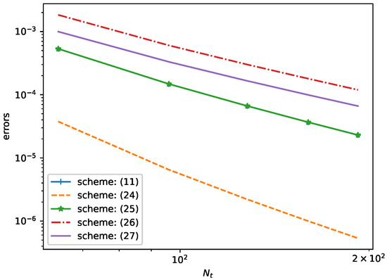
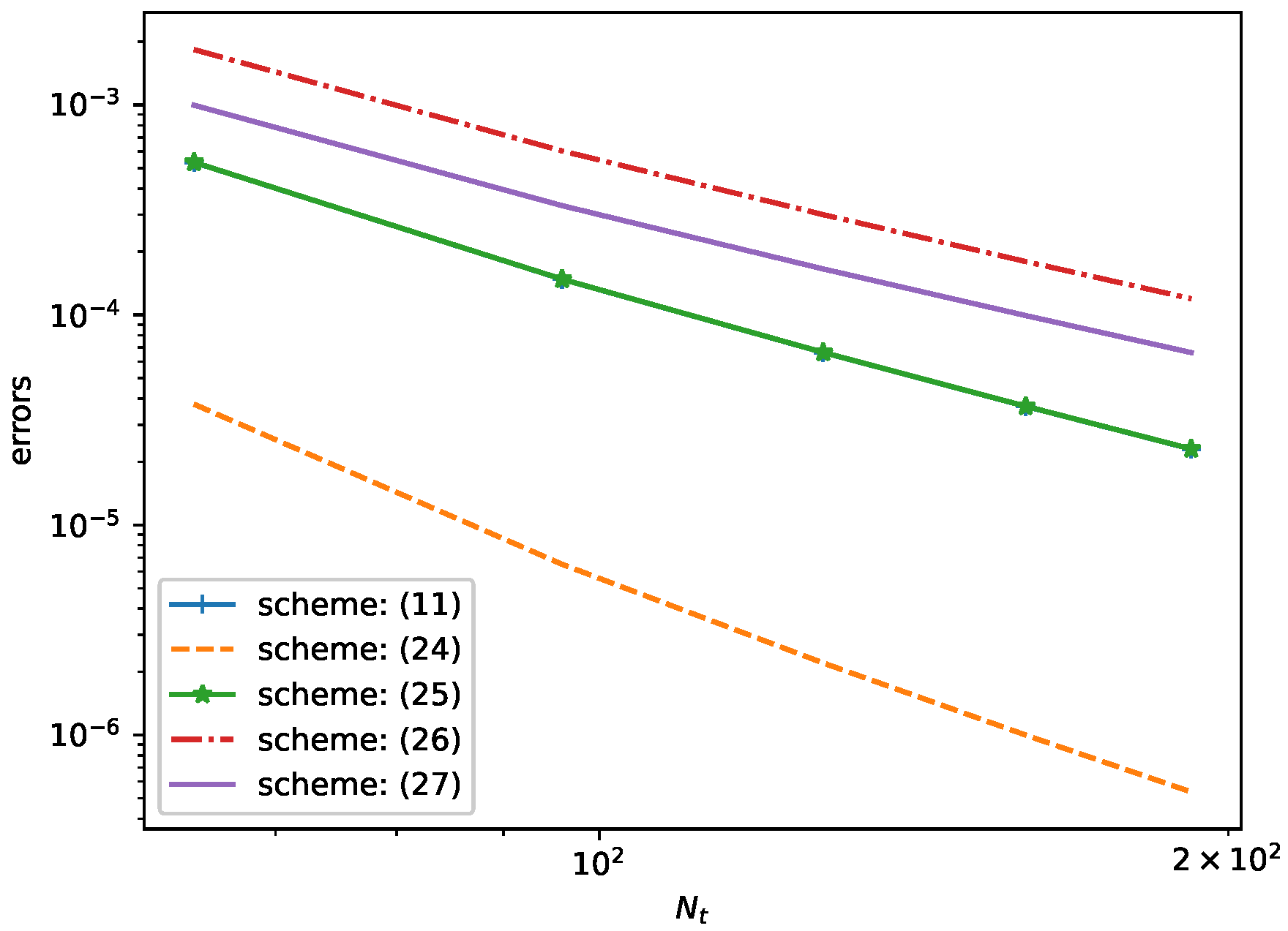
To further demonstrate the superiority of the temporal non-uniform mesh-based compact difference scheme (24) in handling non-smooth solution problems, we compare the $L_2$-norm errors for the five finite difference schemes (11) and (24)–(27) by setting fixed $M_x=1024$ and various $N_t=32,64,96,128,160,192$. Let $N_t^j$ be the jth value of $N_t$, e.g., $N_t^1=32$. The numerical results with errors $E(M_x,N_t^j)={\parallel U^{N_t^j}-U^{N_t^{j-1}}\parallel }_2(j=2,3,\cdots ,6)$ for the case $\alpha =0.3$ are given in Figure 1.

Figure 1. Comparison of the $L_2$-norm errors for different finite difference schemes with fixed $\alpha =0.3$.

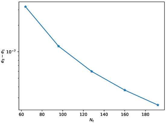
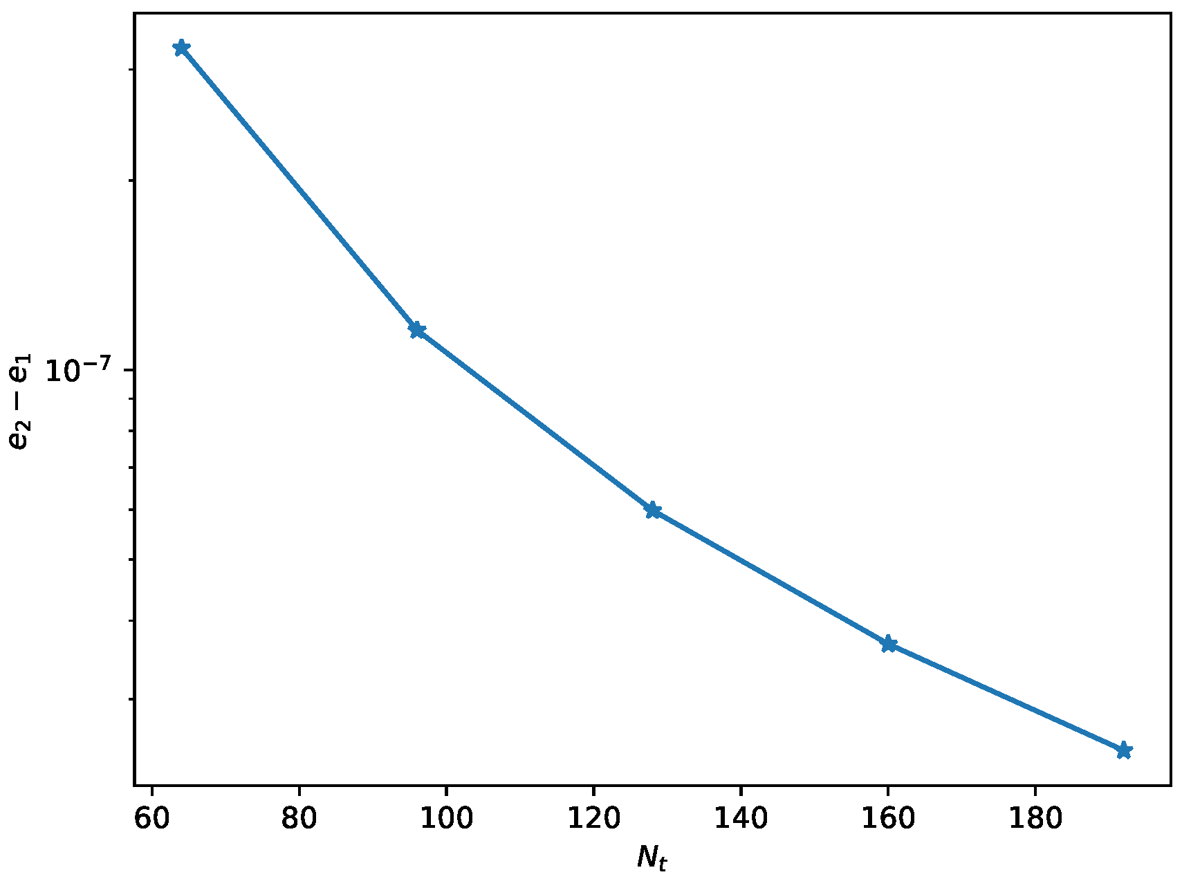
Since the errors of numerical schemes (11) and (25) in Figure 1 are very close to each other, in order to better observe their differences, we let $e_1$ and $e_2$ denote the errors of (11) and (25) respectively, and take their differences $e_2-e_1$ as the vertical coordinates of the axes; see Figure 2.

Figure 2. Subtraction of $L_2$-norm errors for the two different finite difference schemes (11) and (26) with fixed $\alpha =0.3$ (Here, $e_1$ and $e_2$ denote $L_2$-norm errors in (11) and (25), respectively).

As can be seen from Figure 1 and Figure 2, the accuracy of our schemes, particularly the temporal non-uniform mesh-based compact difference scheme (24), is much better than the other three schemes (25)–(27). Similar results are also obtained for the other fractional order α, which are not presented here for the sake of brevity.

Remark 2. 

We remark that for the two non-smooth solution problems Example 2 and the second case of Example 1, the temporal convergence order of the compact difference scheme (11) is different, with Example 2 having the temporal convergence order of $1+\alpha$, while the second case of the previous example has almost $2-\alpha$ in time (see the top lines in Table 3 and Table 5, respectively). Indeed, using the definition and properties of the Mittag–Leffler function (see, e.g., (1.3) in [19]), one can deduce that the solution in Example 2 has the estimate: For $\forall x\in (-2,2),u(x,t)=O(t^{\alpha })$ as $t\to 0^{+}$. It follows that the temporal convergence order of (11) is $1+\alpha$ in view of the error estimate (c) in Theorem 2.5 of [20]. However, the term ${\mathcal{L}}_{x}u(x,t)+f(x,t)$ in the second case of Example 1 has the following form:

$${\mathcal{L}}_{x}u(x,t)+f(x,t)=e^x\left(\Gamma (1+\alpha )+\frac{1}{\Gamma (2-\alpha )}{t}^{1-\alpha }\right).$$

From the Equations (4) and (6), and reusing the error estimate (c) in Theorem 2.5 of [20], one can see that the temporal convergence order in the second case of Example 1 is $2-\alpha$ when the temporal uniform meshes-based compact difference scheme (11) is applied.

Example 3. 

We perform the numerical simulation to study the dynamical behavior of the following time-fractional B-S model which describes the double-barrier knock-out calls:

$$\frac{{\partial }^{\alpha }V}{\partial t^{\alpha }}+\frac{1}{2}{\sigma }^2{S}^2\frac{{\partial }^{2}V}{\partial S^2}+(r-D)S\frac{\partial V}{\partial S}-rV=0,$$

(28)

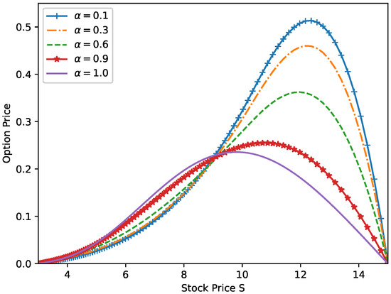
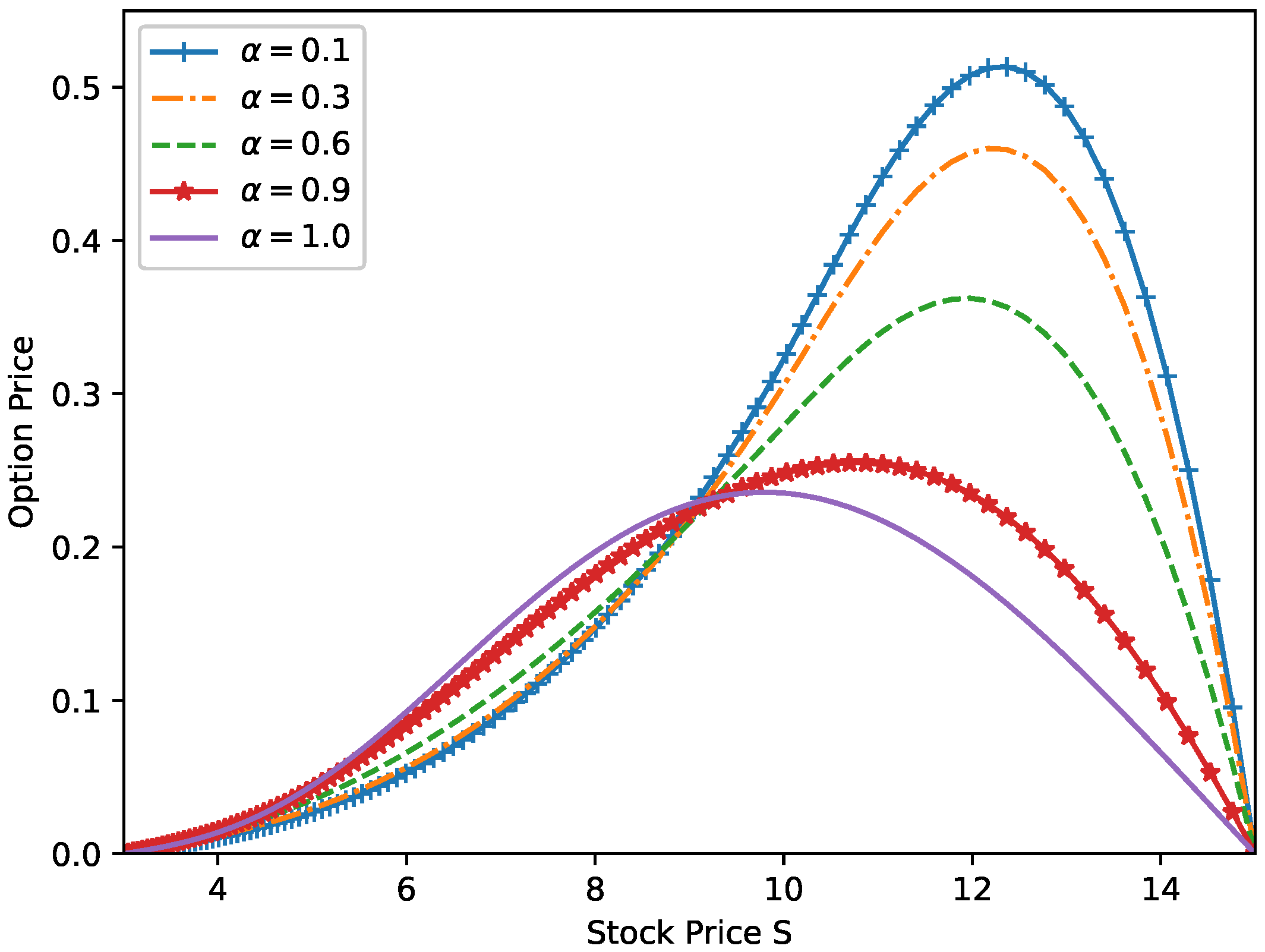
with the boundary conditions $V(S_l,t)=0,V(S_r,t)=0,t\in (0,T)$, and terminal condition $V(S,T)=max\{S-K,0\},S\in (S_l,S_r)$. The parameters of the above equation are considered as $r=0.03,K=10,\sigma =0.45,T=1$ (year), $D=0.01$, and the domain are set as $(S_l,S_r)=(3,15)$. One may refer to [1] for more details. In view of the corresponding equivalent form (2), we employ the temporal non-uniform mesh-based compact difference scheme (24) by setting $N_t=100$ and $M_x=100$ to plot the double-barrier option price at different α; see Figure 3.

Figure 3. Numerical simulation of the double-barrier option prices with different $\alpha$ (Computed by the scheme (24) with $N_t=100$ and $M_x=100$ at $\alpha =0.1,0.3,0.6,0.9$, and $1.0$).

It can be observed from Figure 3 that the fractional order α in the time-fractional B-S Equation (1) has crucial influence on the option price. When the order α is smaller, e.g., $\alpha =0.1$, the option price deviates more from that of classical model. This phenomenon is especially significant when the stock price $S>K$. This coincides with the conclusion of [1] and illustrates the rich expressive power of time-fractional B-S model (1) to characterize option price fluctuations.

6. Conclusions

Since the time-fractional B-S model often has a non-smooth payoff function, i.e., a non-smooth initial condition, the solution to the equation has limited smoothness, making it inherently difficult to construct higher order numerical schemes. In this paper, in order to overcome this difficulty, we investigated the compact difference schemes with temporal uniform/non-uniform meshes. The corresponding stability and error estimate are proved by the method of Fourier analysis. Numerical examples show that the derived schemes are stable with accuracy of $O({\tau }^2+h^4)/O({\tau }_{max}^2+h^4)$ for the smooth/non-smooth solution problem. Thus, we improved some convergence results in the existing literature, in particular the two results presented in [16,18] by fourth-order spatial accuracy and second-order temporal accuracy, respectively, especially for the non-smooth solution problem.

It is known that the practical movement of financial markets is more complicated than that described by the one-dimensional time-fractional B-S model (1). Some researchers have paid close attention to the efficient numerical methods of the high-dimensional B-S model; see [21,22] and the references therein. Thus, it is interesting to extend the ideas of our paper to solving high-dimensional problems, which will be one of our upcoming works.

References

- Chen, W.; Xu, X.; Zhu, S.P. Analytically pricing double barrier options based on a time-fractional Black–Scholes equation. Comput. Math. Appl. 2015, 69, 1407–1419. [Google Scholar] [CrossRef] [Scilit]
- Bekiros, S.; Cardani, R.; Paccagnini, A.; Villa, S. Dealing with financial instability under a DSGE modeling approach with banking intermediation: A predictability analysis versus TVP-VARs. J. Financ. Stab. 2016, 26, 216–227. [Google Scholar] [CrossRef] [Scilit]
- Golbabai, A.; Nikan, O.; Nikazad, T. Numerical analysis of time fractional Black–Scholes European option pricing model arising in financial market. Comput. Appl. Math. 2019, 38, 1–24. [Google Scholar] [CrossRef] [Scilit]
- Fall, A.N.; Ndiaye, S.N.; Sene, N. Black–Scholes option pricing equations described by the Caputo generalized fractional derivative. Chaos Solitons Fractals 2019, 125, 108–118. [Google Scholar] [CrossRef] [Scilit]
- Zhang, H.; Liu, F.; Turner, I.; Yang, Q. Numerical solution of the time fractional Black–Scholes model governing European options. Comput. Math. Appl. 2016, 71, 1772–1783. [Google Scholar] [CrossRef] [Scilit]
- Staelen, R.D.; Hendy, A. Numerically pricing double barrier options in a time-fractional Black–Scholes model. Comput. Math. Appl. 2017, 74, 1166–1175. [Google Scholar] [CrossRef] [Scilit]
- Roul, P. A high accuracy numerical method and its convergence for time-fractional Black-Scholes equation governing European options. Appl. Numer. Math. 2020, 151, 472–493. [Google Scholar] [CrossRef] [Scilit]
- Li, C.; Chen, A. Numerical methods for fractional partial differential equations. Int. J. Comput. Methods 2018, 95, 1048–1099. [Google Scholar] [CrossRef] [Scilit]
- Jin, B.; Lazarov, R.; Zhou, Z. Numerical methods for time-fractional evolution equations with nonsmooth data: A concise overview. Comput. Methods Appl. Mech. Engrg. 2019, 346, 332–358. [Google Scholar] [CrossRef] [Scilit]
- Li, C.; Zeng, F. Numerical Methods for Fractional Calculus; Chapman and Hall/CRC: Boca Raton, FL, USA, 2015. [Google Scholar]
- Li, C.; Yi, Q.; Chen, A. Finite difference methods with non-uniform meshes for nonlinear fractional differential equations. J. Comput. Phys. 2016, 316, 614–631. [Google Scholar] [CrossRef] [Scilit]
- Stynes, M.; O’Riordan, E.; Gracia, J. Error analysis of a finite difference method on graded meshes for a time-fractional diffusion equation. SIAM J. Numer. Anal. 2017, 55, 1057–1079. [Google Scholar] [CrossRef] [Scilit]
- Liao, H.l.; Tang, T.; Zhou, T. An energy stable and maximum bound preserving scheme with variable time steps for time fractional Allen–Cahn equation. SIAM J. Sci. Comput. 2021, 43, A3503–A3526. [Google Scholar] [CrossRef] [Scilit]
- Nong, L.; Yi, Q.; Cao, J.; Chen, A. Fast Compact Difference Scheme for Solving the Two-Dimensional Time-Fractional Cattaneo Equation. Fractal Fract. 2022, 6, 438. [Google Scholar] [CrossRef] [Scilit]
- Cen, Z.; Huang, J.; Xu, A.; Le, A. Numerical approximation of a time-fractional Black–Scholes equation. Comput. Math. Appl. 2018, 75, 2874–2887. [Google Scholar] [CrossRef] [Scilit]
- Kazmi, K. A second order numerical method for the time-fractional Black–Scholes European option pricing model. J. Comput. Appl. Math. 2023, 418, 114647. [Google Scholar] [CrossRef] [Scilit]
- Song, K.; Lyu, P. A high-order and fast scheme with variable time steps for the time-fractional Black-Scholes equation. Math. Methods Appl. Sci. 2022, 46, 1990–2011. [Google Scholar] [CrossRef] [Scilit]
- Roul, P.; Goura, V.P. A compact finite difference scheme for fractional Black-Scholes option pricing model. Appl. Numer. Math. 2021, 166, 40–60. [Google Scholar] [CrossRef] [Scilit]
- Stynes, M. Too much regularity may force too much uniqueness. Fract. Calc. Appl. Anal. 2016, 19, 1554–1562. [Google Scholar] [CrossRef] [Scilit]
- Diethelm, K.; Ford, N.J.; Freed, A.D. Detailed error analysis for a fractional Adams method. Numer. Algorithms 2004, 36, 31–52. [Google Scholar] [CrossRef] [Scilit]
- Chen, W.; Wang, S. A 2nd-order ADI finite difference method for a 2D fractional Black–Scholes equation governing European two asset option pricing. Math. Comput. Simul. 2020, 171, 279–293. [Google Scholar] [CrossRef] [Scilit]
- Zhang, M.; Zhang, G.F. Fast solution method and simulation for the 2D time-space fractional Black-Scholes equation governing European two-asset option pricing. Numer. Algorithms 2022, 91, 1559–1575. [Google Scholar] [CrossRef] [Scilit]
Disclaimer/Publisher’s Note: The statements, opinions and data contained in all publications are solely those of the individual author(s) and contributor(s) and not of MDPI and/or the editor(s). MDPI and/or the editor(s) disclaim responsibility for any injury to people or property resulting from any ideas, methods, instructions or products referred to in the content. |
© 2023 by the authors. Licensee MDPI, Basel, Switzerland. This article is an open access article distributed under the terms and conditions of the Creative Commons Attribution (CC BY) license (https://creativecommons.org/licenses/by/4.0/).