Fractional Gradient Methods via ψ-Hilfer Derivative

Abstract

Motivated by the increase in practical applications of fractional calculus, we study the classical gradient method under the perspective of the $\psi$-Hilfer derivative. This allows us to cover several definitions of fractional derivatives that are found in the literature in our study. The convergence of the $\psi$-Hilfer continuous fractional gradient method was studied both for strongly and non-strongly convex cases. Using a series representation of the target function, we developed an algorithm for the $\psi$-Hilfer fractional order gradient method. The numerical method obtained by truncating higher-order terms was tested and analyzed using benchmark functions. Considering variable order differentiation and step size optimization, the $\psi$-Hilfer fractional gradient method showed better results in terms of speed and accuracy. Our results generalize previous works in the literature.

1. Introduction

The gradient descent method is a classical convex optimization method. It is widely used in many areas of computer science, such as in image processing [1,2], machine learning [3,4,5], and control systems [6]. Its use on a large scale is essentially due to its intuitive structure, ease of implementation, and accuracy. In recent years, there has been an increase in interest in the application of fractional calculus techniques to develop and implement fractional gradient methods (FGM). The first work dealing with such methods is in [2,7], which addresses problems in the fields of signal processing and adaptive learning. The design of fractional least mean squares algorithms is another example of the application of FGM [8,9,10]. Recently, some applications of FGM have focused on artificial intelligence subjects such as machine learning, deep learning, and neural networks (see [11,12,13] and references therein).

Replacing the first-order integer derivative with a fractional derivative in a gradient can improve its convergence, because long-term information can be included. However, there are some convergence issues in the numerical implementation of the FGM because the real extreme value of the target function is not always the same as the fractional extreme value.

In [14], the authors propose a new FGM to overcome this problem, considering an iterative update of the lower limit of integration in the fractional derivative to shorten the memory characteristic presented in the fractional derivative and truncating the higher order terms of the series expansion associated with the target function. Afterward, Wei et al. [15] designed another method involving variable fractional order to solve the convergence problem.

In the field of fractional calculation, several definitions of fractional and derivative integrals varying in their kernel size can be found. This diversity allows certain problems to be tackled with specific fractional operators. To establish a general operator, a $\psi$-fractional integral operator with respect to function $\psi$ was proposed in [16,17], where the kernel depends on a function $\psi$ with specific properties. To incorporate as many fractional derivative definitions as possible into a single formulation, the concept of a fractional derivative of a function with respect to the function $\psi$ was introduced. In 2017, Almeida [18] proposed the $\psi$-Caputo fractional derivative and studied its main properties. A similar approach can be used to define the $\psi$-Riemann–Liouville fractional derivative. In 2018, Sousa and Oliveira [19] unified both definitions using Hilfer’s concept and introduced the $\psi$-Hilfer fractional derivative. This approach offers the flexibility of choosing the differentiation type, as Hilfer’s definition interpolates smoothly between fractional derivatives of Caputo and Riemann–Liouville types. Additionally, by choosing the function $\psi$, we obtain well-known fractional derivatives, such as Caputo, Riemann–Liouville, Hadamard, Katugampola, Chen, Jumarie, Prabhakar, Erdélyi-Kober, and Weyl, among others (see Section 5 in [19]).

The aim of this work is to propose a FGM with a $\psi$-Hilfer fractional derivative. Using this type of general derivative allows us to deal with several fractional derivatives in the literature at the same time. It also allows us to study cases where the target function is a composition of functions. In the first section, we show some auxiliary results concerning the chain rule and solutions of some fractional partial differential equations to study the convergence of the continuous $\psi$-fractional gradient method for strongly and non-strongly convex target functions. In the second section, we introduce and implement numerical algorithms for the $\psi$-Hilfer FGM in one- and two-dimensional cases, generalizing the ideas presented in [14,15]. The proposed algorithms were tested using benchmark functions. The numerical results had better performance compared with the classical gradient in terms of accuracy and number of iterations.

In summary, this paper is organized as follows: in Section 2, we recall some basic concepts about the $\psi$-Hilfer derivative and the two-parameter Mittag–Leffler function. We present some auxiliary results in Section 3, which are then used to analyze the continuous gradient method for strongly and non-strongly convex target functions in Section 4. In the last section of the paper, we design and implement numerical algorithms for the $\psi$-Hilfer FGM by replacing the lower limit of the fractional integral with the last iterate and by using the variable order of differentiation with the optimization of the step size in each iteration. The convergence, accuracy, and speed of the algorithms are analyzed using different examples.

2. General Fractional Derivatives and Special Functions

In this section, we recall some concepts related to fractional integrals and derivatives of a function with respect to another function $\psi$ (for more details, see [16,18,19]).

Definition 1.

(cf. [19], Def. 4) Let $\left[a,b\right]$ be a finite or infinite interval on the real line $\mathbb{R}$ and $\alpha >0$. In addition, let ψ be an increasing and positive monotone function on $\left(a,b\right)$. The left Riemann–Liouville fractional integral of a function f with respect to another function ψ on $\left[a,b\right]$ is defined by

$$\begin{array}{c}\hfill \left(I_{a^{+}}^{\alpha ;\psi }f\right)\left(t\right)=\frac{1}{\Gamma \left(\alpha \right)}{\int }_a^t{\psi }^{\prime }\left(w\right){\left(\psi \left(t\right)-\psi \left(w\right)\right)}^{\alpha -1}f\left(w\right)dw,t>a.\end{array}$$

(1)

Now, we introduce the definition of the so-called $\psi$-Hilfer fractional derivative of a function f with respect to another function.

Definition 2.

(cf. [19], Def. 7) Let $\alpha >0$, $m=\lfloor \alpha \rfloor +1$, and $I=\left[a,b\right]$ be a finite or infinite interval on the real line and $f,\psi \in C^m\left[a,b\right]$ of two functions such that ψ is a positive monotone increasing function and ${\psi }^{\prime }\left(t\right)\ne 0$, for all $t\in I$. The ψ-Hilfer left fractional derivative ${}^H{\mathbb{D}}_{t,a^{+}}^{\alpha ,\mu ;\psi }$ of order α and type $\mu \in \left[0,1\right]$ is defined by

$$\begin{array}{c}\hfill \left({{}^{H}D}_{a^{+}}^{\alpha ,\mu ;\psi }f\right)\left(t\right)=I_{a^{+}}^{\mu \left(m-\alpha \right);\psi }{\left(\frac{1}{{\psi }^{\prime }\left(t\right)}\frac{d}{dt}\right)}^m{I}_{a^{+}}^{\left(1-\mu \right)\left(m-\alpha \right);\psi }f\left(t\right).\end{array}$$

(2)

We observe that when $\mu =0$, we recover the left fractional derivative $\psi$-Riemann–Liouville (see Definition 5 in [19]) and when $\mu =1$, we obtain the left $\psi$-Caputo fractional derivative (see Definition 6 in [19]). The following list shows some fractional derivatives that are encompassed in Definition 2 for specific choices of the function $\psi$ and parameter $\mu :$

• Riemann–Liouville: $\psi \left(t\right)=t$, $I={\mathbb{R}}^{+}$, and $\mu =0$;
• Caputo: $\psi \left(t\right)=t$, $I={\mathbb{R}}^{+}$, and $\mu =1$;
• Katugampola: $\psi \left(t\right)=t^{\rho }$, with $\rho \in {\mathbb{R}}^{+}$, $I={\mathbb{R}}^{+}$, and $\mu =0$;
• Caputo-Katugampola: $\psi \left(t\right)=t^{\rho }$, with $\rho \in {\mathbb{R}}^{+}$, $I={\mathbb{R}}^{+}$, and $\mu =1$;
• Hadamard: $\psi \left(t\right)=ln\left(t\right)$, $I=]1,+\infty [$, and $\mu =0$;
• Caputo-Hadamard: $\psi \left(t\right)=ln\left(t\right)$, $I=]1,+\infty [$, and $\mu =1$.

For a more complete list, please refer to Section 5 in [19]. By considering partial fractional integrals and derivatives, previous definitions can be defined for higher dimensions (see Chapter 5 in [16]). Furthermore, the $\psi$-Hilfer fractional derivative of an n-dimensional vector function $f\left(t\right)=\left(f_1\left(t\right),\dots ,f_n\left(n\right)\right)$ is defined component-wise as

$$\begin{array}{c}\hfill {{}^{H}D}_{a^{+}}^{\alpha ,\mu ;\psi }f\left(t\right)=\left({{}^{H}D}_{a^{+}}^{\alpha ,\mu ;\psi }{f}_1\left(t\right),\dots ,{{}^{H}D}_{a^{+}}^{\alpha ,\mu ;\psi }{f}_n\left(t\right)\right).\end{array}$$

(3)

Next, we present some technical results related to previously introduced operators.

Theorem 1.

(cf. [19], Thm. 5) If $f\in C^m\left[a,b\right]$, $\alpha >0$, $m=\lfloor \alpha \rfloor +1$, and $\mu \in [0,1]$, then

$$\begin{array}{c}\hfill I_{a^{+}}^{\alpha ;\psi }{{}^{H}D}_{a^{+}}^{\alpha ,\mu ;\psi }f\left(t\right)=f\left(t\right)-\sum _{k=1}^m\frac{{\left(\psi \left(t\right)-\psi \left(a\right)\right)}^{\gamma -k}}{\Gamma \left(\gamma -k+1\right)}{f}_{\psi }^{[m-k]}{I}_{a^{+}}^{\left(1-\mu \right)\left(m-\alpha \right);\psi }f\left(a\right),\end{array}$$

(4)

where $\gamma =\alpha +\mu \left(k-\alpha \right)$ and $f_{\psi }^{\left[m\right]}f\left(t\right)={\left(\frac{1}{{\psi }^{\prime }\left(t\right)}\frac{d}{dt}\right)}^{m}f\left(t\right).$

Lemma 1.

(cf. [19], Lem. 5) Given $\delta \in \mathbb{R}$, consider the function $f\left(t\right)={\left(\psi \left(t\right)-\psi \left(a\right)\right)}^{\delta -1}$, where $\delta >m$. Then, for $m=\lfloor \alpha \rfloor +1$ and $\mu \in \left[0,1\right]$, we have

$$\begin{array}{c}\hfill {{}^{H}D}_{a^{+}}^{\alpha ,\mu ;\psi }f\left(x\right)=\frac{\Gamma \left(\delta \right)}{\Gamma \left(\delta -\alpha \right)}{\left(\psi \left(t\right)-\psi \left(a\right)\right)}^{\delta -\alpha -1}.\end{array}$$

(5)

Some results of the paper are given in terms of the two-parameter Mittag–Leffler function, which is defined by the following power series (see [20])

$$\begin{array}{c}\hfill E_{{\beta }_1,{\beta }_2}\left(z\right)=\sum _{n=0}^{+\infty }\frac{z^n}{\Gamma \left({\beta }_{1}n+{\beta }_2\right)},\mathrm{Re}\left({\beta }_1\right)>0,{\beta }_2\in \mathbb{C},z\in \mathbb{C}.\end{array}$$

For $z=-x,$ with $x\in {\mathbb{R}}^{+},$$0<{\beta }_1<2,$ and ${\beta }_2\in \mathbb{C},$ the two-parameter Mittag–Leffler function has the following asymptotic expansion (see Equation (4.7.36) in [20]):

$$\begin{array}{c}\hfill E_{{\beta }_1,{\beta }_2}\left(-x\right)=-\sum _{k=1}^p\frac{{\left(-x\right)}^{-k}}{\Gamma \left({\beta }_2-{\beta }_{1}k\right)}+O\left({\left|x\right|}^{-1-p}\right),p\in \mathbb{N},x\to +\infty .\end{array}$$

(6)

3. Auxiliary Results

In this section, we present some auxiliary results needed for our work. These extend some results presented in [21] to the $\psi$-Hilfer derivative of arbitrary type $\mu \in [0,1]$.

We start by presenting a representation formula for the solution of a Cauchy problem involving the $\psi$-Hilfer derivative. Let us consider $h:{\mathbb{R}}_0^{+}\times {\mathbb{R}}^n\to {\mathbb{R}}^n$ and $f:\mathbb{R}\to {\mathbb{R}}^n$. We obtain the following results.

Proposition 1.

Let $\alpha \in [0,1]$ and $\mu \in \left[0,1\right]$. A continuous function f is a solution of the problem

$$\begin{array}{c}\hfill \left\{\begin{array}{cc}\hfill & {{}^{H}D}_{a^{+}}^{\alpha ,\mu ;\psi }f\left(t\right)=h\left(t,f\left(t\right)\right),t\ge a,\hfill \\ \hfill & I_{a^{+}}^{\left(1-\alpha \right)\left(1-\mu \right);\psi }f\left(a^{+}\right)=f_a\hfill \end{array}\right.\end{array}$$

(7)

if and only if f is given by

$$\begin{array}{cc}\hfill f\left(t\right)& =\frac{f_a}{\Gamma \left(\alpha +\mu \left(1-\alpha \right)\right)}{\left(\psi \left(t\right)-\psi \left(a\right)\right)}^{\alpha +\mu \left(1-\alpha \right)-1}\hfill \\ \hfill & +\frac{1}{\Gamma \left(\alpha \right)}{\int }_a^t{\left(\psi \left(t\right)-\psi \left(s\right)\right)}^{\alpha -1}{\psi }^{\prime }\left(s\right)h\left(s,f\left(s\right)\right)ds,t\ge a.\hfill \end{array}$$

(8)

Proof. 

Applying $I_{a^{+}}^{\alpha ;\psi }$ to both sides of the fractional differential equation in (7), and taking (4) with $m=1$, we have

$$\begin{array}{c}\hfill I_{a^{+}}^{\alpha ;\psi }{{}^{H}D}_{a^{+}}^{\alpha ,\mu ;\psi }f\left(t\right)=f\left(t\right)-\frac{f_a}{\Gamma \left(\alpha +\mu \left(1-\alpha \right)\right)}{\left(\psi \left(t\right)-\psi \left(a\right)\right)}^{\alpha +\mu \left(1-\alpha \right)-1}\end{array}$$

which is equivalent to

$$\begin{array}{c}\hfill f\left(t\right)=\frac{f_a}{\Gamma \left(\alpha +\mu \left(1-\alpha \right)\right)}{\left(\psi \left(t\right)-\psi \left(a\right)\right)}^{\alpha +\mu \left(1-\alpha \right)-1}+I_{a^{+}}^{\alpha ;\psi }{{}^{H}D}_{a^{+}}^{\alpha ,\mu ;\psi }f\left(t\right).\end{array}$$

From (1) and (7), we obtain these results.    □

Now, we present some results concerning the fractional derivative of a composite function. Let us consider $g:{\mathbb{R}}^n\to \mathbb{R}$, $f:\mathbb{R}\to {\mathbb{R}}^n$, ∇ as the classical gradient operator, and the $\psi$-Hilfer fractional derivative of an n-dimensional vector function as (3).

Theorem 2.

Let $\alpha \in [0,1]$, $\mu \in [0,1]$, $a\ge 0$, and the function ψ to be in the conditions of Definition 2. For $t>a$, let us define the function ${\zeta }_t$ by setting

$$\begin{array}{c}\hfill {\zeta }_t\left(s\right)=g\left(f\left(s\right)\right)-g\left(f\left(t\right)\right)-⟨\left(\nabla g\right)\left(f\left(t\right)\right),f\left(s\right)-f\left(t\right)⟩,\end{array}$$

(9)

where

$$\begin{array}{c}\hfill \left(\nabla g\right)\left(f\left(t\right)\right)=\left(\frac{\partial g}{\partial x_1}\left(f\left(t\right)\right),\dots ,\frac{\partial g}{\partial x_n}\left(f\left(t\right)\right)\right).\end{array}$$

The following identity holds

$$\begin{array}{cc}\hfill & \Gamma \left(1-\alpha \right)\left({{}^{H}D}_{a^{+}}^{\alpha ,\mu ;\psi }\left[g\left(f\left(t\right)\right)\right]-⟨\left(\nabla g\right)\left(f\left(t\right)\right),{{}^{H}D}_{a^{+}}^{\alpha ,\mu ;\psi }f\left(t\right)⟩\right)\hfill \\ \hfill & ={\left[\psi \left(t\right)-\psi \left(a\right)\right]}^{-\alpha }\left[g\left(f\left(t\right)\right)-⟨\left(\nabla g\right)\left(f\left(t\right)\right),f\left(t\right)⟩\right]\hfill \\ \hfill & -\alpha {\int }_a^t{\left(\psi \left(t\right)-\psi \left(s\right)\right)}^{-\alpha -1}{\psi }^{\prime }\left(s\right){\zeta }_t\left(s\right)ds.\hfill \end{array}$$

(10)

Proof. 

By the Newton–Leibniz formula, for each component of the function f, one has

$$\begin{array}{c}\hfill f_i\left(t\right)=f_i\left(a\right)+{\int }_a^t{f}_i^{\prime }\left(s\right)ds=f_i\left(a\right)+I_{a^{+}}^{1;\psi }\left(\frac{f_i^{\prime }}{{\psi }^{\prime }}\right)\left(t\right),i=1,\dots ,n.\end{array}$$

From (3), for $i=1,\dots ,n$, we have

$$\begin{array}{cc}\hfill {{}^{H}D}_{a^{+}}^{\alpha ,\mu ;\psi }{f}_i\left(t\right)& ={{}^{H}D}_{a^{+}}^{\alpha ,\mu ;\psi }\left[f_i\left(a\right)\right]\left(t\right)+{{}^{H}D}_{a^{+}}^{\alpha ,\mu ;\psi }\circ I_{a^{+}}^{1;\psi }\left(\frac{f_i^{\prime }}{{\psi }^{\prime }}\right)\left(t\right)\hfill \\ \hfill & =I_{a^{+}}^{\mu \left(1-\alpha \right);\psi }\left[\frac{1}{{\psi }^{\prime }\left(t\right)}\frac{d}{dt}\right]I_{a^{+}}^{\left(1-\mu \right)\left(1-\alpha \right);\psi }\left[f_i\left(a\right)\right]\left(t\right)\hfill \\ \hfill & +I_{a^{+}}^{\mu \left(1-\alpha \right);\psi }\left[\frac{1}{{\psi }^{\prime }\left(t\right)}\frac{d}{dt}\right]I_{a^{+}}^{\left(1-\mu \right)\left(1-\alpha \right);\psi }{I}_{a^{+}}^{1;\psi }\left(\frac{f_i^{\prime }}{{\psi }^{\prime }}\right)\left(t\right)\hfill \\ \hfill & =f_i\left(a\right)I_{a^{+}}^{\mu \left(1-\alpha \right);\psi }\left[\frac{1}{{\psi }^{\prime }\left(t\right)}\frac{d}{dt}\right]I_{a^{+}}^{\left(1-\mu \right)\left(1-\alpha \right);\psi }\left[1\right]\left(t\right)\hfill \\ \hfill & +I_{a^{+}}^{\mu \left(1-\alpha \right);\psi }\left[\frac{1}{{\psi }^{\prime }\left(t\right)}\frac{d}{dt}\right]I_{a^{+}}^{\left(1-\mu \right)\left(1-\alpha \right)+1;\psi }\left(\frac{f_i^{\prime }}{{\psi }^{\prime }}\right)\left(t\right).\hfill \end{array}$$

(11)

Taking (1) into account, the first term in (11) is

$$\begin{array}{cc}\hfill & f_i\left(a\right)I_{a^{+}}^{\mu \left(1-\alpha \right);\psi }\left[\frac{1}{{\psi }^{\prime }\left(t\right)}\frac{d}{dt}\right]I_{a^{+}}^{\left(1-\mu \right)\left(1-\alpha \right);\psi }\left[1\right]\left(t\right)\hfill \\ \hfill & =f_i\left(a\right)I_{a^{+}}^{\mu \left(1-\alpha \right);\psi }\left[\frac{1}{{\psi }^{\prime }\left(t\right)}\frac{d}{dt}\right]\frac{1}{\Gamma \left(\left(1-\mu \right)\left(1-\alpha \right)\right)}{\int }_a^t{\left(\psi \left(t\right)-\psi \left(s\right)\right)}^{\left(1-\mu \right)\left(1-\alpha \right)-1}{\psi }^{\prime }\left(s\right)ds\hfill \\ \hfill & =f_i\left(t\right)I_{a^{+}}^{\mu \left(1-\alpha \right);\psi }\left[\frac{1}{{\psi }^{\prime }\left(t\right)}\frac{d}{dt}\right]\left[\frac{{\left(\psi \left(t\right)-\psi \left(a\right)\right)}^{\left(1-\mu \right)\left(1-\alpha \right)}}{\Gamma \left(\left(1-\mu \right)\left(1-\alpha \right)+1\right)}\right]\hfill \\ \hfill & =\frac{f_i\left(a\right)}{\Gamma \left(\mu \left(1-\alpha \right)\right)}{\int }_a^t{\left(\psi \left(t\right)-\psi \left(s\right)\right)}^{\mu \left(1-\alpha \right)-1}\frac{{\left(\psi \left(s\right)-\psi \left(a\right)\right)}^{\left(1-\mu \right)\left(1-\alpha \right)-1}}{\Gamma \left(\left(1-\mu \right)\left(1-\alpha \right)\right)}{\psi }^{\prime }\left(s\right)ds\hfill \\ \hfill & =\frac{f_i\left(a\right)}{\Gamma \left(1-\alpha \right)}{\left(\psi \left(t\right)-\psi \left(a\right)\right)}^{-\alpha }.\hfill \end{array}$$

(12)

For the second term in (11), taking (1) and the Leibniz rule for differentiation under the integral sign into account, we obtain

$$\begin{array}{cc}\hfill & I_{a^{+}}^{\mu \left(1-\alpha \right);\psi }\left[\frac{1}{{\psi }^{\prime }\left(t\right)}\frac{d}{dt}\right]I_{a^{+}}^{\left(1-\mu \right)\left(1-\alpha \right)+1;\psi }\left(\frac{f_i^{\prime }}{{\psi }^{\prime }}\right)\left(t\right)\hfill \\ \hfill & =I_{a^{+}}^{\mu \left(1-\alpha \right);\psi }\left[\frac{1}{{\psi }^{\prime }\left(t\right)}\frac{d}{dt}\right]\frac{1}{\Gamma \left(\left(1-\mu \right)\left(1-\alpha \right)+1\right)}{\int }_a^t{\left(\psi \left(t\right)-\psi \left(s\right)\right)}^{\left(1-\mu \right)\left(1-\alpha \right)}{f}_i^{\prime }\left(s\right)ds\hfill \\ \hfill & =I_{a^{+}}^{\mu \left(1-\alpha \right);\psi }\frac{1}{\Gamma \left(\left(1-\mu \right)\left(1-\alpha \right)\right)}{\int }_a^t{\left(\psi \left(t\right)-\psi \left(s\right)\right)}^{\left(1-\mu \right)\left(1-\alpha \right)-1}{f}_i^{\prime }\left(s\right)ds\hfill \\ \hfill & =I_{a^{+}}^{\mu \left(1-\alpha \right);\psi }{I}_{a^{+}}^{\left(1-\mu \right)\left(1-\alpha \right);\psi }\left(\frac{f_i^{\prime }}{{\psi }^{\prime }}\right)\left(t\right)\hfill \\ \hfill & =\frac{1}{\Gamma \left(1-\alpha \right)}{\int }_a^t{\left(\psi \left(t\right)-\psi \left(s\right)\right)}^{-\alpha }{f}_i^{\prime }\left(s\right)ds.\hfill \end{array}$$

(13)

From (12) and (13), expression (11) simplifies to

$$\begin{array}{cc}\hfill & {{}^{H}D}_{a^{+}}^{\alpha ,\mu ;\psi }{f}_i\left(t\right)\hfill \\ \hfill & =\frac{1}{\Gamma \left(1-\alpha \right)}\left[f_i\left(a\right){\left(\psi \left(t\right)-\psi \left(a\right)\right)}^{-\alpha }+{\int }_a^t{\left(\psi \left(t\right)-\psi \left(s\right)\right)}^{-\alpha }{f}_i^{\prime }\left(s\right)ds\right],i=1,\dots ,n\hfill \end{array}$$

and therefore,

$$\begin{array}{c}\hfill {{}^{H}D}_{a^{+}}^{\alpha ,\mu ;\psi }f\left(t\right)=\frac{1}{\Gamma \left(1-\alpha \right)}\left[f\left(a\right){\left(\psi \left(t\right)-\psi \left(a\right)\right)}^{-\alpha }+{\int }_a^t{\left(\psi \left(t\right)-\psi \left(s\right)\right)}^{-\alpha }{f}^{\prime }\left(s\right)ds\right].\end{array}$$

(14)

Hence, we can write

$$\begin{array}{cc}\hfill & \Gamma \left(1-\alpha \right)\left({{}^{H}D}_{a^{+}}^{\alpha ,\mu ;\psi }\left[g\left(f\left(t\right)\right)\right]-⟨\left(\nabla g\right)\left(f\left(t\right)\right),{{}^{H}D}_{a^{+}}^{\alpha ,\mu ;\psi }f\left(t\right)⟩\right)\hfill \\ \hfill & ={\left[\psi \left(t\right)-\psi \left(a\right)\right]}^{-\alpha }\left[g\left(f\left(a\right)\right)-⟨\left(\nabla g\right)\left(f\left(t\right)\right),f\left(a\right)⟩\right]\hfill \\ \hfill & +{\int }_a^t{\left(\psi \left(t\right)-\psi \left(s\right)\right)}^{-\alpha }⟨\left(\nabla g\right)\left(f\left(s\right)\right)-\left(\nabla g\right)\left(f\left(t\right)\right),f^{\prime }\left(s\right)⟩ds\hfill \\ \hfill & ={\left[\psi \left(t\right)-\psi \left(a\right)\right]}^{-\alpha }\left[g\left(f\left(a\right)\right)-⟨\left(\nabla g\right)\left(f\left(t\right)\right),f\left(a\right)⟩\right]\hfill \\ \hfill & +{\int }_a^t{\left(\psi \left(t\right)-\psi \left(s\right)\right)}^{-\alpha }d{\zeta }_t\left(s\right)\hfill \end{array}$$

(15)

which implies, by integrating by parts, that

$$\begin{array}{cc}\hfill & \Gamma \left(1-\alpha \right)\left({{}^{H}D}_{a^{+}}^{\alpha ,\mu ;\psi }\left[g\left(f\left(t\right)\right)\right]-⟨\left(\nabla g\right)\left(f\left(t\right)\right),{{}^{H}D}_{a^{+}}^{\alpha ,\mu ;\psi }f\left(t\right)⟩\right)\hfill \\ \hfill & ={\left[\psi \left(t\right)-\psi \left(a\right)\right]}^{-\alpha }\left[g\left(f\left(a\right)\right)-⟨\left(\nabla g\right)\left(f\left(t\right)\right),f\left(a\right)⟩\right]\hfill \\ \hfill & +\underset{s\to t}{lim}{\left[\psi \left(t\right)-\psi \left(s\right)\right]}^{-\alpha }{\zeta }_t\left(s\right)-{\left[\psi \left(t\right)-\psi \left(a\right)\right]}^{-\alpha }{\zeta }_t\left(a\right)\hfill \\ \hfill & -\alpha {\int }_a^t{\left(\psi \left(t\right)-\psi \left(a\right)\right)}^{-\alpha -1}{\psi }^{\prime }\left(s\right){\zeta }_t\left(s\right)ds.\hfill \end{array}$$

(16)

As $\alpha \in [0,1]$, we have by L’Hôpital’s rule that

$$\begin{array}{c}\hfill \underset{s\to t}{lim}{\left[\psi \left(t\right)-\psi \left(s\right)\right]}^{-\alpha }{\zeta }_t\left(s\right)=\underset{s\to t}{lim}\frac{{\zeta }_t\left(s\right)}{{\left[\psi \left(t\right)-\psi \left(s\right)\right]}^{\alpha }}=\underset{s\to t}{lim}\frac{{\zeta }_t^{\prime }\left(s\right){\left[\psi \left(t\right)-\psi \left(s\right)\right]}^{1-\alpha }}{-\alpha {\psi }^{\prime }\left(s\right)}=0.\end{array}$$

(17)

Finally, from (17) and (9), we obtain the following from (16)

$$\begin{array}{cc}\hfill & \Gamma \left(1-\alpha \right)\left({{}^{H}D}_{a^{+}}^{\alpha ,\mu ;\psi }\left[g\left(f\left(t\right)\right)\right]-⟨\left(\nabla g\right)\left(f\left(t\right)\right),{{}^{H}D}_{a^{+}}^{\alpha ,\mu ;\psi }f\left(t\right)⟩\right)\hfill \\ \hfill & ={\left[\psi \left(t\right)-\psi \left(a\right)\right]}^{-\alpha }\left[{\zeta }_t\left(a\right)-g\left(f\left(t\right)\right)-⟨\left(\nabla g\right)\left(f\left(t\right)\right),f\left(t\right)⟩-{\zeta }_t\left(a\right)\right]\hfill \\ \hfill & -\alpha {\int }_a^t{\left(\psi \left(t\right)-\psi \left(s\right)\right)}^{-\alpha -1}{\psi }^{\prime }\left(s\right){\zeta }_t\left(s\right)ds,\hfill \end{array}$$

which gives the desired result.    □

Corollary 1.

Let $\alpha \in [0,1]$, $\mu \in [0,1]$, $a\ge 0$, and the function ψ have the conditions of Definition 2. If $g:{\mathbb{R}}^n\to \mathbb{R}$ is of class $C^1$ and convex, i.e.,

$$\begin{array}{c}\hfill g\left(x\right)\ge g\left(y\right)+⟨\nabla g\left(x\right),x-y⟩,forallx,y\in {\mathbb{R}}^n,\end{array}$$

(18)

then

$$\begin{array}{c}\hfill {{}^{H}D}_{a^{+}}^{\alpha ,\mu ;\psi }g\left(f\left(t\right)\right)\le ⟨\left(\nabla g\right)\left(f\left(t\right)\right),{{}^{H}D}_{a^{+}}^{\alpha ,\mu ;\psi }f\left(t\right)⟩+\frac{g\left(0\right)}{\Gamma \left(1-\alpha \right)}{\left(\psi \left(t\right)-\psi \left(a\right)\right)}^{-\alpha }.\end{array}$$

(19)

Proof. 

From (18), it follows that for $x=0$,

$$\begin{array}{c}\hfill g\left(f\left(t\right)\right)-⟨\left(\nabla g\right)\left(f\left(t\right)\right),f\left(t\right)⟩\le g\left(0\right)-⟨\left(\nabla g\right)\left(f\left(t\right)\right),0⟩=g\left(0\right).\end{array}$$

On the other hand, based on Theorem 2, we have the following for $x=0$

$$\begin{array}{cc}\hfill & g\left(f\left(t\right)\right)-⟨\left(\nabla g\right)\left(f\left(t\right)\right),f\left(t\right)⟩\hfill \\ \hfill & =\Gamma \left(1-\alpha \right){\left[\psi \left(t\right)-\psi \left(a\right)\right]}^{\alpha }\left({{}^{H}D}_{a^{+}}^{\alpha ,\mu ;\psi }\left[g\left(f\left(t\right)\right)\right]-⟨\left(\nabla g\right)\left(f\left(t\right)\right),{{}^{H}D}_{a^{+}}^{\alpha ,\mu ;\psi }f\left(t\right)⟩\right).\hfill \end{array}$$

Combining the two previous expressions, we obtain our results.    □

If we consider $\mu =0$, which corresponds to the $\psi$-Riemann–Liouville case, the previous results reduce to Proposition 3.3 and Corollary 3.4 in [21], respectively. Moreover, the correspondent results for the $\psi$-Caputo case ($\mu =1$) are presented in Proposition 3.1 of [21].

Now, we present an auxiliary result involving the two-parameter Mittag–Leffler function.

Proposition 2.

Let $\alpha \in [0,1]$, $\mu \in [0,1]$, and $a\ge 0$. Moreover, let ψ be in the conditions of Definition 2, such that $sup\left\{\psi \left(t\right):t\ge a\right\}=+\infty$. Then, the following limit holds

$$\begin{array}{c}\hfill \underset{t\to +\infty }{lim}{\int }_a^t{\left(\psi \left(t\right)-\psi \left(a\right)\right)}^{\alpha -1}{\psi }^{\prime }\left(s\right)E_{\alpha ,\alpha +\mu \left(1-\alpha \right)}\left(-\lambda {\left(\psi \left(s\right)-\psi \left(a\right)\right)}^{\alpha }\right)ds=0.\end{array}$$

Proof. 

Taking into account Theorem 5.1 in [22] for the case of a homogeneous equation, the solution of the initial value problem

$$\begin{array}{c}\hfill \left\{\begin{array}{cc}\hfill & {{}^{H}D}_{a^{+}}^{\alpha ,\mu ;\psi }u\left(t\right)=-\lambda u\left(t\right);\lambda \in {\mathbb{R}}^{+},\alpha \in [0,1],\mu \in [0,1],t\ge a\hfill \\ \hfill & I_{a^{+}}^{1-\alpha -\mu \left(1-\alpha \right);\psi }u\left(a\right)=u_a\hfill \end{array}\right.\end{array}$$

is given by

$$\begin{array}{c}\hfill u\left(t\right)={\left(\psi \left(t\right)-\psi \left(a\right)\right)}^{\alpha -\mu \left(1-\alpha \right)-1}{E}_{\alpha ,\alpha +\mu \left(1-\alpha \right)}\left(-\lambda {\left(\psi \left(t\right)-\psi \left(a\right)\right)}^{\alpha }\right).\end{array}$$

Hence, by Proposition 1, we have

$$\begin{array}{cc}\hfill & E_{\alpha ,\alpha \mu \left(1-\alpha \right)}\left(-\lambda {\left(\psi \left(t\right)-\psi \left(a\right)\right)}^{\alpha }\right)\hfill \\ \hfill & =\frac{u_a}{\Gamma \left(\alpha +\mu \left(1-\alpha \right)\right)}{\left(\psi \left(t\right)-\psi \left(a\right)\right)}^{\alpha +\mu \left(1-\alpha \right)-1}\hfill \\ \hfill & -\frac{\lambda }{\Gamma \left(\alpha \right)}{\int }_a^t{\left(\psi \left(t\right)-\psi \left(s\right)\right)}^{\alpha -1}{\psi }^{\prime }\left(s\right)E_{\alpha ,\alpha +\mu \left(1-\alpha \right)}\left(-\lambda {\left(\psi \left(s\right)-\psi \left(a\right)\right)}^{\alpha }\right)ds.\hfill \end{array}$$

Taking the limit when $t\to +\infty$ on both sides and considering the asymptotic expansion (6), we conclude that the left-hand side tends to approach zero and the first term of the right-hand side also tends to approach zero. Hence, we obtain

$$\begin{array}{c}\hfill 0=0-\frac{\lambda }{\Gamma \left(\alpha \right)}{\int }_a^t{\left(\psi \left(t\right)-\psi \left(s\right)\right)}^{\alpha -1}{\psi }^{\prime }\left(s\right)E_{\alpha ,\alpha +\mu \left(1-\alpha \right)}\left(-\lambda {\left(\psi \left(s\right)-\psi \left(a\right)\right)}^{\alpha }\right)ds\end{array}$$

which leads to our results.    □

The case when $\mu =1$, i.e., the $\psi$-Caputo case, was already studied in [21] and corresponds to Lemma 3.7.

4. Continuous Gradient Method via the $\mathbf{\psi }$-Hilfer Derivative

Assume that we aim to determine the minimum of a function $f:{\mathbb{R}}^n\to \mathbb{R}$. To achieve this, the gradient descent method is used, starting with an initial prediction $x_0$ of the local minimum and producing a sequence $x_0,x_1,x_2,\dots$ based on the following recurrence relation:

$$\begin{array}{c}\hfill x_{k+1}=x_k-{\theta }_k\nabla f\left(x_k\right),\end{array}$$

(20)

where the step size $\theta >0$ is either constant or varying at each iteration k. The sequence ${\left\{x_k\right\}}_{k=0}^{+\infty }$ generated by the gradient descent method is monotonic, i.e., $f\left(x_0\right)>f\left(x_1\right)>f\left(x_2\right)>\dots$, and is expected to converge to a local minimum of f. Typically, the stopping criterion is in the form $∥\nabla f\left(x\right)∥\le ϵ$, where $ϵ>0$. By expressing (20) as

$$\begin{array}{c}\hfill \frac{x_{k+1}-x_k}{{\theta }_k}=-\nabla f\left(x_k\right),\end{array}$$

(21)

we can interpret (21) as the discretization of the initial value problem

$$\begin{array}{c}\hfill y^{\prime }\left(t\right)=-\left(\nabla f\right)\left(y\left(t\right)\right),y\left(0\right)=y_0\in {\mathbb{R}}^n,\end{array}$$

(22)

using the explicit Euler scheme with step size ${\theta }_k$. The system (22) is known as the continuous gradient method (see [21]). Assuming that f is both strongly convex and smooth, the solutions of (20) and (22) converge to the unique stationary point at an exponential rate. In general, if a convergence result is shown for a continuous method, then we can construct various finite difference schemes for the solution of the associated Cauchy problem. Let us now consider the following $\psi$-fractional version of (22)

$$\begin{array}{c}\hfill {{}^{H}D}_{a^{+}}^{\alpha ,\mu ;\psi }z\left(t\right)=-\theta \left(\nabla f\right)\left(z\left(t\right)\right),t\ge a,\end{array}$$

(23)

such that $z:\mathbb{R}\to {\mathbb{R}}^n$, $f:{\mathbb{R}}^n\to \mathbb{R}$, $\alpha \in [0,1]$, $\mu \in [0,1]$, and $I_{a^{+}}^{1-\alpha ;\psi }z\left(a^{+}\right)=z_a\in {\mathbb{R}}^n$, where the last expression is evaluated at the limit $t\to a^{+}$. For $y^{*}\in S\left(f\right)=\left\{z\in {\mathbb{R}}^n:\nabla f\left(z\right)=0\right\}$, let us define the following sum of squares error function:

$$\begin{array}{c}\hfill \phi \left(t\right)=\frac{1}{2}{∥z\left(t\right)-y^{*}∥}^2,t\ge a.\end{array}$$

(24)

4.1. The Convex Case

Here, we investigate (23) under the assumption of non-strongly convexity of f.

Theorem 3.

Let $\alpha \in [0,1]$ and $\mu \in [0,1]$. Suppose that the function $f:{\mathbb{R}}^n\to \mathbb{R}$ is of class $C^1$ and convex, i.e., f satisfies (18). For the ψ-fractional differential Equation (23), with step size θ constant, the solution $z\left(·\right)$ converges to $y^{*}$ with the upper bound

$$\begin{array}{c}\hfill {∥z\left(t\right)-y^{*}∥}^2\le C{\left|\psi \left(t\right)-\psi \left(a\right)\right|}^{-\mu \left(1-\alpha \right)},\mathit{for}\mathit{all}t\ge a.\end{array}$$

(25)

Proof. 

Based on Corollary 1 applied to (24) and the fact that f is of class $C^1$ and convex, we have

$$\begin{array}{cc}\hfill {{}^{H}D}_{a^{+}}^{\alpha ,\mu ;\psi }\phi \left(t\right)& \le -\theta ⟨z\left(t\right)-y^{*},\left(\nabla f\right)\left(z\left(t\right)\right)⟩\hfill \\ \hfill & \le \theta \left[f\left(y^{*}\left(t\right)\right)-f\left(z\left(t\right)\right)\right]\le 0,\mathrm{for}\mathrm{all}t\ge a.\hfill \end{array}$$

By the properties of $\psi$ (see Definition 2), the previous expression is equivalent to

$$\begin{array}{c}\hfill I_{a^{+}}^{\alpha ;\psi }{{}^{H}D}_{a^{+}}^{\alpha ,\mu ;\psi }\phi \left(t\right)\le \theta I_{a^{+}}^{\alpha ;\psi }\left[f\left(y^{*}\left(t\right)\right)-f\left(z\left(t\right)\right)\right]\le 0.\end{array}$$

Using the composition rule (4), with $m=1$, we have

$$\begin{array}{c}\hfill \phi \left(t\right)-\frac{{\left(\psi \left(t\right)-\psi \left(a\right)\right)}^{-\mu \left(1-\alpha \right)}}{\Gamma \left(1-\mu \left(1-\alpha \right)\right)}{I}_{a^{+}}^{\left(1-\mu \right)\left(1-\alpha \right);\psi }\phi \left(a^{+}\right)\le 0.\end{array}$$

From (24) and considering $C=\frac{1}{\Gamma \left(1-\mu \left(1-\alpha \right)\right)}{I}_{a^{+}}^{\left(1-\mu \right)\left(1-\alpha \right);\psi }\phi \left(a^{+}\right)$, we obtain our results.    □

If we consider $\mu =0$ in the previous result, we recover Theorem 4.2 in [21].

4.2. The Strongly Convex Case

Here, we show that under the assumption of strong convexity of the function f, the solution of (23) admits a Mittag–Leffler convergence, which is a general type of exponential convergence to the stationary point. Recall the definition of a strongly convex function.

Definition 3.

(cf. [21]) A function $f\in C^1$ is strongly convex with parameter $m_f>0$ if

$$\begin{array}{c}\hfill f\left(x\right)\ge f\left(y\right)+⟨\nabla f\left(y\right),x-y⟩+\frac{m_f}{2}{∥x-y∥}^2,\mathit{for}\mathit{all}x,y\in {\mathbb{R}}^n,\end{array}$$

where ∇ stands for the gradient operator.

Theorem 4.

Let $\alpha \in [0,1]$ and $\mu \in [0,1]$. Suppose that f is of class $C^2$ and is strongly convex. Considering the ψ-fractional differential Equation (23), where the step size θ is a constant, then the solution $z\left(·\right)$ converges to $y^{*}$, with the upper bound

$$\begin{array}{c}\hfill {∥z\left(t\right)-y^{*}∥}^2\le {\phi }_a{\left[\psi \left(t\right)-\psi \left(a\right)\right]}^{(\alpha -1)(1-\mu )}{E}_{\alpha ,\alpha +\mu \left(1-\alpha \right)}\left(-\theta m_f{\left(\psi \left(t\right)-\psi \left(a\right)\right)}^{\alpha }\right),t\ge a,\end{array}$$

where ${\phi }_a=\frac{1}{2}{I}_{a^{+}}^{\left(1-\mu \right)\left(1-\alpha \right);\psi }{∥z\left(t\right)-y^{*}∥}^2\left(a^{+}\right)$.

Proof. 

In Definition 3, if we consider $y=z\left(t\right)$ and $x=y^{*}$, we have for $t\ge a$ and $m_f>0$ that

$$\begin{array}{c}\hfill f\left(y^{*}\right)\ge f\left(z\left(t\right)\right)-⟨\left(\nabla f\right)\left(z\left(t\right)\right),y^{*}-z\left(t\right)⟩+\frac{m_f}{2}{∥y^{*}-z\left(t\right)∥}^2,\end{array}$$

which is equivalent to

$$\begin{array}{cc}\hfill & ⟨\left(\nabla f\right)\left(z\left(t\right)\right),y^{*}-z\left(t\right)⟩\ge f\left(z\left(t\right)\right)-f\left(y^{*}\right)+\frac{m_f}{2}{∥y^{*}-z\left(t\right)∥}^2\ge \frac{m_f}{2}{∥y^{*}-z\left(t\right)∥}^2,\hfill \end{array}$$

(26)

where the last inequality holds, as $y^{*}\in arg\left({min}_{x\in {\mathbb{R}}^n}f\left(x\right)\right)$. From (23), Corollary 1, and (26), we have

$$\begin{array}{cc}\hfill {{}^{H}D}_{a^{+}}^{\alpha ,\mu ;\psi }\phi \left(t\right)& \le ⟨z\left(t\right)-y^{*},{{}^{H}D}_{a^{+}}^{\alpha ,\mu ;\psi }z\left(t\right)⟩\hfill \\ \hfill & =-\theta ⟨z\left(t\right)-y^{*},\left(\nabla f\right)\left(z\left(t\right)\right)⟩\hfill \\ \hfill & \le -\frac{\theta m_f}{2}{∥z\left(t\right)-y^{*}∥}^2.\hfill \end{array}$$

(27)

Setting

$$\begin{array}{c}\hfill h\left(t\right)=-\frac{\theta m_f}{2}{∥z\left(t\right)-y^{*}∥}^2-{{}^{H}D}_{a^{+}}^{\alpha ,\mu ;\psi }\phi \left(t\right),\end{array}$$

(28)

we have from (27) that $h\left(t\right)\ge 0$ for all $t\ge a$, and moreover, from (28) and recalling (24), the previous expression is equivalent to

$$\begin{array}{c}\hfill {{}^{H}D}_{a^{+}}^{\alpha ,\mu ;\psi }\phi \left(t\right)=-\theta m_f\phi \left(t\right)-h\left(t\right).\end{array}$$

(29)

By Theorem 5.1 in [22], we have that the solution of (29) is

$$\begin{array}{cc}\hfill \phi \left(t\right)& ={\phi }_a{\left[\psi \left(t\right)-\psi \left(a\right)\right]}^{\alpha +\mu \left(1-\alpha \right)-1}{E}_{\alpha ,\alpha +\mu \left(1-\alpha \right)}\left(-\theta m_f{\left(\psi \left(t\right)-\psi \left(a\right)\right)}^{\alpha }\right)\hfill \end{array}$$

$$\begin{array}{cc}\hfill & -{\int }_a^t{\left(\psi \left(t\right)-\psi \left(a\right)\right)}^{\alpha -1}{\psi }^{\prime }\left(w\right)E_{\alpha ,\alpha }\left(-\theta m_f{\left(\psi \left(t\right)-\psi \left(a\right)\right)}^{\alpha }\right)h\left(w\right)dw\hfill \end{array}$$

(30)

$$\begin{array}{cc}\hfill & \le {\phi }_a{\left[\psi \left(t\right)-\psi \left(a\right)\right]}^{\alpha +\mu \left(1-\alpha \right)-1}{E}_{\alpha ,\alpha +\mu \left(1-\alpha \right)}\left(-\theta m_f{\left(\psi \left(t\right)-\psi \left(a\right)\right)}^{\alpha }\right),\hfill \end{array}$$

(31)

where the last inequality holds, as the integrand function in (30) is positive and $0\le a<t$.    □

4.3. Convergence at an Exponential Rate

Theorem 4 establishes the Mittag–Leffler convergence rate for the solution of (23) to a stationary point. Specifically, when $\alpha =1$, the exponential rate $O\left(e^{-\theta ,m_f\psi \left(t\right)}\right)$ of the continuous gradient method (22) is recovered for any $\mu \in [0,1]$.

Theorem 5.

Let $\alpha \in [0,1]$, $\mu \in [0,1]$, and ψ satisfy the conditions of Definition 2 with $sup\left\{\psi \left(t\right):t\ge a\right\}=+\infty$. Let $f:{\mathbb{R}}^n\to \mathbb{R}$ be a function that is $C^1$, convex, and Lipschitz smooth with constant $L_f$, that is,

$$\begin{array}{c}\hfill ∥\nabla f\left(x\right)-\nabla f\left(y\right)∥\le L_f∥x-y∥,\mathit{for}\mathit{all}x,y\in {\mathbb{R}}^n.\end{array}$$

(32)

If the solution $z\left(·\right)$ of (23) converges to $y^{*}$ at the exponential rate $O\left(e^{-\omega \psi \left(t\right)}\right)$, then $y^{*}=0$.

Proof. 

Let $z\left(·\right)$ be a solution of (23) converging to the stationary point $y^{*}$ at the rate $O\left(e^{-\omega \psi \left(t\right)}\right)$. Then, there exists a $t_1$ greater or equal to a, such that

$$\begin{array}{c}\hfill ∥z\left(t\right)-y^{*}∥\le e^{-\omega \psi \left(t\right)},\mathrm{for}\mathrm{all}t\ge t_1.\end{array}$$

(33)

By contradiction, let us assume that $y^{*}\ne 0$. We can then set

$$\begin{array}{c}\hfill k=\frac{\theta }{∥y^{*}∥}+1.\end{array}$$

(34)

From Formula (4.11.4b) in [20],

$$\begin{array}{c}\hfill E_{\alpha ,\beta }\left(z\right)=2E_{2\alpha ,\beta }\left(z^2\right)-E_{\alpha ,\beta }\left(-z\right),\mathrm{Re}\left(\alpha \right)>0,\beta \in \mathbb{C},\end{array}$$

(35)

we can find $t_2\ge t_1$ with the property that

$$\begin{array}{c}\hfill E_{\alpha ,\beta }\left(-L_f{\left(\psi \left(t\right)-\psi \left(a\right)\right)}^{\alpha }\right)\ge k{e}^{-\omega \psi \left(t\right)},\mathrm{for}\mathrm{all}t\ge t_2.\end{array}$$

(36)

By Proposition 1, $z\left(·\right)$ is of the following form

$$\begin{array}{cc}\hfill z\left(t\right)& =\frac{z_a}{\Gamma \left(\alpha +\mu \left(1-\alpha \right)\right)}{\left(\psi \left(t\right)-\psi \left(a\right)\right)}^{\alpha +\mu \left(1-\alpha \right)-1}\hfill \\ \hfill & -\frac{\theta }{\Gamma \left(\alpha \right)}{\int }_a^t{\left(\psi \left(t\right)-\psi \left(s\right)\right)}^{\alpha -1}{\psi }^{\prime }\left(s\right)\left(\nabla f\right)\left(z\left(s\right)\right)ds,\hfill \end{array}$$

which is equivalent to

$$\begin{array}{cc}\hfill & z_a{\left(\psi \left(t\right)-\psi \left(a\right)\right)}^{\alpha +\mu \left(1-\alpha \right)-1}\hfill \\ \hfill & =\Gamma \left(\alpha +\mu \left(1-\alpha \right)\right)z\left(t\right)\hfill \\ \hfill & +\frac{\theta \Gamma \left(\alpha +\mu \left(1-\alpha \right)\right)}{\Gamma \left(\alpha \right)}{\int }_a^t{\left(\psi \left(t\right)-\psi \left(s\right)\right)}^{\alpha -1}{\psi }^{\prime }\left(s\right)\left(\nabla f\right)\left(z\left(s\right)\right)ds.\hfill \end{array}$$

(37)

Setting

$$\begin{array}{cc}\hfill & u\left(t\right)=z_a{\left(\psi \left(t\right)-\psi \left(a\right)\right)}^{\alpha +\mu \left(1-\alpha \right)-1}-\Gamma \left(\alpha +\mu \left(1-\alpha \right)\right)y^{*},\hfill \end{array}$$

then, by (37), we obtain

$$\begin{array}{cc}\hfill ∥u\left(t\right)∥& =∥z_a{\left(\psi \left(t\right)-\psi \left(a\right)\right)}^{\alpha +\mu \left(1-\alpha \right)-1}-\Gamma \left(\alpha +\mu \left(1-\alpha \right)\right)y^{*}∥\hfill \\ \hfill & \le \Gamma \left(\alpha +\mu \left(1-\alpha \right)\right)∥z\left(t\right)-y^{*}∥\hfill \\ \hfill & +\frac{\theta \Gamma \left(\alpha +\mu \left(1-\alpha \right)\right)}{\Gamma \left(\alpha \right)}{\int }_a^t{\left(\psi \left(t\right)-\psi \left(s\right)\right)}^{\alpha -1}{\psi }^{\prime }\left(s\right)∥\left(\nabla f\right)\left(z\left(s\right)\right)∥ds.\hfill \end{array}$$

By assumption (32), we obtain

$$\begin{array}{cc}\hfill & ∥u\left(t\right)∥\hfill \\ \hfill & \le \Gamma \left(\alpha +\mu \left(1-\alpha \right)\right)∥z\left(t\right)-y^{*}∥\hfill \\ \hfill & +\frac{\theta L_f\Gamma \left(\alpha +\mu \left(1-\alpha \right)\right)}{\Gamma \left(\alpha \right)}{\int }_a^t{\left(\psi \left(t\right)-\psi \left(s\right)\right)}^{\alpha -1}{\psi }^{\prime }\left(s\right)∥z\left(t\right)-y^{*}∥ds\hfill \end{array}$$

$$\begin{array}{cc}\hfill & =\Gamma \left(\alpha +\mu \left(1-\alpha \right)\right)∥z\left(t\right)-y^{*}∥\hfill \\ \hfill & +\frac{\theta L_f\Gamma \left(\alpha +\mu \left(1-\alpha \right)\right)}{\Gamma \left(\alpha \right)}{\int }_a^{t_2}{\left(\psi \left(t\right)-\psi \left(s\right)\right)}^{\alpha -1}{\psi }^{\prime }\left(s\right)∥z\left(t\right)-y^{*}∥ds\hfill \\ \hfill & +\frac{\theta L_f\Gamma \left(\alpha +\mu \left(1-\alpha \right)\right)}{\Gamma \left(\alpha \right)}{\int }_{t_2}^t{\left(\psi \left(t\right)-\psi \left(s\right)\right)}^{\alpha -1}{\psi }^{\prime }\left(s\right)∥z\left(t\right)-y^{*}∥ds.\hfill \end{array}$$

(38)

Now, denoting $Q=sup\left\{∥z\left(·\right)-y^{*}∥:t\in [a,t_2]\right\}$ and using (36), we obtain

$$\begin{array}{cc}\hfill & ∥u\left(t\right)∥\hfill \\ \hfill & \le \Gamma \left(\alpha +\mu \left(1-\alpha \right)\right)∥z\left(t\right)-y^{*}∥\hfill \\ \hfill & +\frac{\theta L_{f}Q\Gamma \left(\alpha +\mu \left(1-\alpha \right)\right)}{\Gamma \left(\alpha \right)}{\int }_a^{t_2}{\left(\psi \left(t\right)-\psi \left(s\right)\right)}^{\alpha -1}{\psi }^{\prime }\left(s\right)ds\hfill \\ \hfill & +\frac{\theta L_f\Gamma \left(\alpha +\mu \left(1-\alpha \right)\right)}{\Gamma \left(\alpha \right)}{\int }_{t_2}^t{\left(\psi \left(t\right)-\psi \left(s\right)\right)}^{\alpha -1}{\psi }^{\prime }\left(s\right)E_{\alpha ,\alpha +\mu \left(1-\alpha \right)}\left(-L_f{\left(\psi \left(s\right)-\psi \left(a\right)\right)}^{\alpha }\right)ds\hfill \\ \hfill & =\Gamma \left(\alpha +\mu \left(1-\alpha \right)\right)∥z\left(t\right)-y^{*}∥\hfill \\ \hfill & +\frac{\theta L_{f}Q\Gamma \left(\alpha +\mu \left(1-\alpha \right)\right)}{\alpha \Gamma \left(\alpha \right)}\left[{\left(\psi \left(t\right)-\psi \left(a\right)\right)}^{\alpha }-{\left(\psi \left(t\right)-\psi \left(t_2\right)\right)}^{\alpha }\right]\hfill \\ \hfill & +\frac{\theta L_f\Gamma \left(\alpha +\mu \left(1-\alpha \right)\right)}{\Gamma \left(\alpha \right)}{\int }_{t_2}^t{\left(\psi \left(t\right)-\psi \left(s\right)\right)}^{\alpha -1}{\psi }^{\prime }\left(s\right)E_{\alpha ,\alpha +\mu \left(1-\alpha \right)}\left(-L_f{\left(\psi \left(s\right)-\psi \left(a\right)\right)}^{\alpha }\right)ds.\hfill \end{array}$$

By the mean value theorem (applied to the function ${\left(\psi \left(t\right)-\psi \left(·\right)\right)}^{\alpha }$), there exists $\delta \in ]a,t_2[$ such that

$$\begin{array}{c}\hfill {\left(\psi \left(t\right)-\psi \left(a\right)\right)}^{\alpha }-{\left(\psi \left(t\right)-\psi \left(t_2\right)\right)}^{\alpha }=-\alpha {\left(\psi \left(t\right)-\psi \left(\delta \right)\right)}^{\alpha -1}{\psi }^{\prime }\left(\delta \right)\end{array}$$

which implies that, as $\alpha \in [0,1]$ and $sup\left\{\psi \left(t\right):t\ge a\right\}=+\infty$,

$$\begin{array}{cc}\hfill & \underset{t\to +\infty }{lim}\left[{\left(\psi \left(t\right)-\psi \left(a\right)\right)}^{\alpha }-{\left(\psi \left(t\right)-\psi \left(t_2\right)\right)}^{\alpha }\right]\hfill \\ \hfill & =-\alpha \underset{t\to +\infty }{lim}\left[{\left(\psi \left(t\right)-\psi \left(\delta \right)\right)}^{\alpha -1}{\psi }^{\prime }\left(\delta \right)\right]\hfill \\ \hfill & =-\alpha \underset{t\to +\infty }{lim}\frac{{\psi }^{\prime }\left(\delta \right)}{{\left(\psi \left(t\right)-\psi \left(\delta \right)\right)}^{1-\alpha }}=0.\hfill \end{array}$$

(39)

Hence, taking the limit of $∥u\left(t\right)∥$ when $t\to +\infty$, we obtain

$$\begin{array}{c}\hfill \underset{t\to +\infty }{lim}∥u\left(t\right)∥=0\iff \Gamma \left(\alpha +\mu \left(1-\alpha \right)\right)∥y^{*}∥=0.\end{array}$$

This implies that $∥y^{*}∥=0$, which is a contradiction.    □

5. $\mathbf{\psi }$-Hilfer Fractional Gradient Method

The aim of this section is to construct and implement a numerical method for the $\psi$-Hilfer FGM in one- and two-dimensional cases. For both cases, we perform numerical simulations using benchmark functions.

5.1. The One-Dimensional Case

5.1.1. Design of the Numerical Method

The gradient descent method typically takes steps proportional to the negative gradient (or approximate gradient) of a function at the current iteration, that is, $x_{k+1}$ is updated by the following law

$$\begin{array}{c}\hfill x_{k+1}=x_k-\theta f^{\prime }\left(x_k\right),k=0,1,2,\dots ,\end{array}$$

(40)

where $\theta >0$ is the step size or learning rate, and $f^{\prime }\left(x_k\right)$ is the first derivative of f evaluated at $x=x_k$. We assume that $f:\mathbb{R}\to \mathbb{R}$ admits a local minimum at the point $x^{*}$ in ${\mathbb{D}}_{\rho }\left(x^{*}\right)=\left\{x\in \mathbb{R}:\left|x-x^{*}\right|<\rho \right\}$, for some $\rho >0$, and f admits a Taylor series expansion centered at $x_0=a$,

$$\begin{array}{c}\hfill f\left(x\right)=\sum _{p=0}^{+\infty }\frac{f^{\left(p\right)}\left(a\right)}{p!}{\left(x-a\right)}^p,\end{array}$$

(41)

with domain of convergence $D\subseteq \mathbb{R}$ such that $X^{*}\in D$. As we want to consider the fractional gradient in the $\psi$-Hilfer sense, our first (and natural attempt) is to consider the iterative method

$$\begin{array}{c}\hfill x_{k+1}=x_k-\theta {{}^{H}D}_{a^{+}}^{\alpha ,\mu ;\psi }f\left(\psi \left(x_k\right)\right),k=0,1,2,\dots ,\end{array}$$

(42)

where ${{}^{H}D}_{a^{+}}^{\alpha ,\mu ;\psi }$ is the $\psi$-Hilfer derivative of order $\alpha \in ]0,1[$ and type $\mu \in [0,1]$, given by (2), and the function $\psi$ is in the conditions of Definition 2. However, a simple example shows that (42) is not the correct approach. In fact, let us consider the quadratic function $f\left(x\right)={(x-h)}^2$ with a minimum at $x^{*}=h$. For this function, we have that

$$\begin{array}{c}\hfill {{}^{H}D}_{a^{+}}^{\alpha ,\mu ;\psi }f\left(x\right)=\sum _{p=p_0}^2\frac{f^{\left(p\right)}\left(a\right)}{\Gamma \left(p+1-\alpha \right)}{\left(x-a\right)}^{p-\alpha },\end{array}$$

(43)

where $p_0=0$ if $\mu \in [0,1]$ and $p_0=1$ if $\mu =1$. As ${{}^{H}D}_{a^{+}}^{\alpha ,\mu ;\psi }f\left(h\right)\ne 0$, the iterative method (42) does not converge to the real minimum point. This example shows that the $\psi$-Hilfer FGM with a fixed lower limit of integration does not converge to the minimum point. This is due to the influence of long-time memory terms, which is an intrinsic feature of fractional derivatives. In order to address this problem and inspired by the ideas presented in [14,15], we replace the starting point a in the fractional derivative by the term $x_{k-1}$ of the previous iteration, that is,

$$\begin{array}{c}\hfill x_{k+1}=x_k-\theta {{}^{H}D}_{x_{k-1}^{+}}^{\alpha ,\mu ;\psi }f\left(\psi \left(x_k\right)\right),k=1,2,\dots \end{array}$$

(44)

where $\alpha \in ]0,1[$, $\mu \in [0,1]$, and $\theta >0$. This eliminates the long-time memory effect during the iteration procedure. In this sense, and taking into account the series representation (41) and differentiation rule (5), we obtain

$$\begin{array}{c}\hfill {{}^{H}D}_{x_{k-1}^{+}}^{\alpha ,\mu ;\psi }f\left(\psi \left(x_k\right)\right)=\sum _{p=p_0}^{+\infty }\frac{f^{\left(p\right)}\left(\psi \left(x_{k-1}\right)\right)}{\Gamma \left(p+1-\alpha \right)}{\left(\psi \left(x_k\right)-\psi \left(x_{k-1}\right)\right)}^{p-\alpha },\end{array}$$

(45)

where $p_0=0$ if $\mu \in [0,1]$ or $p_0=1$ if $\mu =1$. Thus, the representation formula (45) depends only on $\mu =1$ or $\mu \ne 1.$ With this modification in the $\psi$-Hilfer FGM, we obtain the following convergence results.

Theorem 6.

If the algorithm (44) is convergent, with the fractional gradient given by (45), then it converges to the minimum point of $f\left(\psi \left(·\right)\right)$.

Proof. 

Let $x^{*}$ be the minimum point of $f\left(\psi \left(·\right)\right)$. We prove that the sequence ${\left(x_k\right)}_{k\in \mathbb{N}}$ converges to $x^{*}$ by contradiction. Assume that $x_k$ converges to a different $x\ne x^{*}$ and $f^{\prime }\left(\psi \left(x\right)\right)\ne 0$. As the algorithm is convergent, we have that ${lim}_{k\to +\infty }∥x_k-x∥=0$. Moreover, for any small positive $ϵ$, there exists a sufficiently large number $N\in \mathbb{N}$, such that

$$\begin{array}{c}\hfill \left|\psi \left(x_{k-1}\right)-\psi \left(x\right)\right|<ϵ<\left|\psi \left(x^{*}\right)-\psi \left(x\right)\right|\end{array}$$

(46)

for any $k>N$. Thus,

$$\begin{array}{c}\hfill \delta =\underset{p>N}{inf}\left|f^{\left(p_0\right)}\left(\psi \left(x_{k-1}\right)\right)\right|>0\end{array}$$

must hold. From (45) we have

$$\begin{array}{cc}\hfill \left|x_{k+1}-x_k\right|& =\theta \left|{{}^{H}D}_{x_{k-1}^{+}}^{\alpha ,\mu ;\psi }f\left(\psi \left(x_k\right)\right)\right|\hfill \\ \hfill & =\theta \left|\sum _{p=0}^{+\infty }\frac{f^{\left(p+p_0\right)}\left(\psi \left(x_{k-1}\right)\right)}{\Gamma \left(p+p_0+1-\alpha \right)}{\left(\psi \left(x_k\right)-\psi \left(x_{k-1}\right)\right)}^{p+p_0-\alpha }\right|\hfill \\ \hfill & \ge \theta \left|\frac{f^{\left(p_0\right)}\left(\psi \left(x_{k-1}\right)\right)}{\Gamma \left(p_0+1-\alpha \right)}{\left(\psi \left(x_k\right)-\psi \left(x_{k-1}\right)\right)}^{p_0-\alpha }\right|\hfill \\ \hfill & -\theta \left|\sum _{p=1}^{+\infty }\frac{f^{\left(p+p_0\right)}\left(\psi \left(x_{k-1}\right)\right)}{\Gamma \left(p+p_0+1-\alpha \right)}{\left(\psi \left(x_k\right)-\psi \left(x_{k-1}\right)\right)}^{p+p_0-\alpha }\right|.\hfill \end{array}$$

Considering

$$\begin{array}{c}\hfill C=\underset{p\ge N}{sup}\frac{\left|f^{\left(p_0\right)}\left(\psi \left(x_{k-1}\right)\right)\right|}{\Gamma \left(p_0+1-\alpha \right)},\end{array}$$

(47)

we have, from the previous expression,

$$\begin{array}{cc}\hfill \left|x_{k+1}-x_k\right|& \ge \theta \left|\frac{f^{\left(p_0\right)}\left(\psi \left(x_{k-1}\right)\right)}{\Gamma \left(p_0+1-\alpha \right)}{\left(\psi \left(x_k\right)-\psi \left(x_{k-1}\right)\right)}^{p_0-\alpha }\right|\hfill \\ \hfill & -\theta C\sum _{p=1}^{+\infty }|\psi \left(x_k\right)-\psi \left(x_{k-1}\right){|}^{p+p_0-\alpha }.\hfill \end{array}$$

The geometric series in the previous expression is convergent for sufficiently large k. Hence, we obtain

$$\begin{array}{cc}\hfill \left|x_{k+1}-x_k\right|& \ge \theta \left|\frac{f^{\left(p_0\right)}\left(\psi \left(x_{k-1}\right)\right)}{\Gamma \left(p_0+1-\alpha \right)}{\left(\psi \left(x_k\right)-\psi \left(x_{k-1}\right)\right)}^{p_0-\alpha }\right|\hfill \\ \hfill & -\theta C\frac{{\left|\psi \left(x_k\right)-\psi \left(x_{k-1}\right)\right|}^{1+p_0-\alpha }}{1-\left|\psi \left(x_k\right)-\psi \left(x_{k-1}\right)\right|},\hfill \end{array}$$

which is equivalent to

$$\begin{array}{cc}\hfill & \left|x_{k+1}-x_k\right|\hfill \\ \hfill & \ge \theta \left[\left|\frac{f^{\left(p_0\right)}\left(\psi \left(x_{k-1}\right)\right)}{\Gamma \left(p_0+1-\alpha \right)}\right|-C\frac{\left|\psi \left(x_k\right)-\psi \left(x_{k-1}\right)\right|}{1-\left|\psi \left(x_k\right)-\psi \left(x_{k-1}\right)\right|}\right]{\left|\psi \left(x_k\right)-\psi \left(x_{k-1}\right)\right|}^{p_0-\alpha }\hfill \end{array}$$

$$\begin{array}{cc}\hfill & \ge d{\left|\psi \left(x_k\right)-\psi \left(x_{k-1}\right)\right|}^{p_0-\alpha },\hfill \end{array}$$

(48)

where

$$\begin{array}{c}\hfill d=d\left(ϵ\right)=\theta \left[\frac{\delta }{\Gamma \left(p_0+1-\alpha \right)}-\frac{2Cϵ}{1-ϵ}\right].\end{array}$$

(49)

One can always find $ϵ$ sufficiently small, such that

$$\begin{array}{c}\hfill \frac{\delta }{\Gamma \left(p_0+1-\alpha \right)}-\frac{2Cϵ}{1-ϵ}>\frac{2{ϵ}^{\alpha }}{\theta }\iff \frac{\delta }{\Gamma \left(p_0+1-\alpha \right)}>\frac{2{ϵ}^{\alpha }}{\theta }+\frac{2Cϵ}{1-ϵ}\end{array}$$

(50)

because the function $g\left(ϵ\right)=\frac{2{ϵ}^{\alpha }}{\theta }+\frac{2Cϵ}{1-ϵ}$ is positively increasing for $\alpha \in [0,1]$, $\theta \in [0,1]$, and $ϵ\in [0,1]$. Hence, from (48) and taking into account (50), we obtain

$$\begin{array}{c}\hfill \left|x_{k+1}-x_k\right|>2{ϵ}^{p_0}=\left\{\begin{array}{cc}2ϵ,\hfill & \mathrm{if}\mu =1\hfill \\ 2,\hfill & \mathrm{if}\mu \in [0,1]\hfill \end{array}\right..\end{array}$$

(51)

On the other hand, from the assumption (46), we have

$$\begin{array}{c}\hfill \left|x_{k+1}-x_k\right|\le \left|\psi \left(x_{k+1}\right)-\psi \left(x_k\right)\right|\le \left|\psi \left(x_{k+1}\right)-\psi \left(x\right)\right|+\left|\psi \left(x\right)-\psi \left(x_k\right)\right|=2ϵ,\end{array}$$

which contradicts (51). This completes the proof.    □

Sometimes, the function f is not smooth enough to admit a series representation in the form (41), and therefore, the implementation of (44) using the series (45) is not possible. For implementation in practice, we need to truncate the series. In our first approach, we consider only the term of the series containing $f^{\prime }\left(\psi \left(x_k\right)\right)$, as it is the most relevant for the gradient method. Thus, the $\psi$-Hilfer FGM (44) simplifies to

$$\begin{array}{c}\hfill x_{k+1}=x_k-\theta \frac{f^{\prime }\left(\psi \left(x_{k-1}\right)\right)}{\Gamma \left(2-\alpha \right)}{\left(\psi \left(x_k\right)-\psi \left(x_{k-1}\right)\right)}^{1-\alpha }.\end{array}$$

(52)

Furthermore, in order to avoid the appearance of complex numbers, we introduce the modulus in the expression (52), that is,

$$\begin{array}{c}\hfill x_{k+1}=x_k-\theta \frac{f^{\prime }\left(\psi \left(x_{k-1}\right)\right)}{\Gamma \left(2-\alpha \right)}{\left|\psi \left(x_k\right)-\psi \left(x_{k-1}\right)\right|}^{1-\alpha }.\end{array}$$

(53)

The pseudocode associated to (53) is presented in Algorithm 1. As (53) is independent of the $\mu$ parameter, from now on we call the method $\psi$-FGM. Following the same arguments as in the proof of Theorem 6, we obtain the following results.

Theorem 7.

If the algorithm (44) is convergent with the fractional gradient given by (53), then it converges to the minimum point of $f\left(\psi \left(·\right)\right)$.

In the following pseudocode, we describe the implementation of the algorithm (53).

Algorithm 1:$\psi$-FGM with higher order truncation.

As we have seen, it is possible to construct a $\psi$-FGM that converges to the minimum point of a function. To improve the convergence of the proposed method, we can consider variable order differentiation $\alpha \left(x\right)$ in each iteration. Some examples of $\alpha \left(x\right)$ are given by (see [15]):

$$\begin{array}{cc}\hfill & \alpha \left(x\right)=\frac{1}{1+\beta J\left(x\right)},\hfill \end{array}$$

(54)

$$\begin{array}{cc}\hfill & \alpha \left(x\right)=\frac{2}{1+e^{\beta J\left(x\right)}},\hfill \end{array}$$

(55)

$$\begin{array}{cc}\hfill & \alpha \left(x\right)=\frac{1}{cos\left(\beta J\left(x\right)\right)},\hfill \end{array}$$

(56)

$$\begin{array}{cc}\hfill & \alpha \left(x\right)=1-\frac{2}{\pi }arctan\left(\beta J\left(x\right)\right),\hfill \end{array}$$

(57)

$$\begin{array}{cc}\hfill & \alpha \left(x\right)=1-tanh\left(\beta J\left(x\right)\right),\hfill \end{array}$$

(58)

where $\beta >0$ and we consider the loss function $J\left(x\right)={\left(f^{\prime }\left(\psi \left(x\right)\right)\right)}^2$ to be minimized in each iteration. The consideration of the square in the loss function guarantees its non-negativity. All examples given satisfy

$$\begin{array}{c}\hfill \underset{\beta \to 0}{lim}\alpha \left(x\right)=1=\underset{x\to x^{*}}{lim}\alpha \left(x\right),\end{array}$$

(59)

where the second limit results from the fact that $J\left(x\right)\to 0$ as $x\to x^{*}.$ Variable order differentiation turns the $\psi$-FGM into a learning method, because as x gradually approaches $x^{*}$, $\alpha \left(x\right)\approx 1.$ The $\psi$-FGM with variable order is given by

$$\begin{array}{c}\hfill x_{k+1}=x_k-\theta \frac{f^{\prime }\left(\psi \left(x_{k-1}\right)\right)}{\Gamma \left(2-\alpha \left(x_k\right)\right)}{\left|\psi \left(x_k\right)-\psi \left(x_{k-1}\right)\right|}^{1-\alpha \left(x_k\right)}.\end{array}$$

Theorem 6 remains valid for this variation of Algorithm 1.

5.1.2. Numerical Simulations

Now, we provide some examples that show the validity of the previous algorithms applied to the quadratic function $f\left(x\right)={\left(x-1\right)}^2$, which is one of the simplest benchmark functions. This function is a convex function with a unique global minimum at $x^{*}=1$. For the $\psi$-derivative, we consider the following cases:

• Caputo and Riemann–Liouville fractional derivatives: ${\psi }_1\left(x\right)=x$, $I=[0,+\infty [$, and $a=0$;
• Hadamard fractional derivative: ${\psi }_2\left(x\right)=ln\left(x\right)$, $I=[1,+\infty [$, and $a=1$;
• Katugampola fractional derivative: ${\psi }_3\left(x\right)=x^{0.5}$, $I=[0,+\infty [$, and $a=0.5$. In this case, a cannot coincide with the lower limit of the interval I because ${\psi }^{\prime }$ is not defined at $x=0$.

Figure 1, Figure 2 and Figure 3 show the numerical results of Algorithm 1 applied to the composite functions $f\left({\psi }_1\left(·\right)\right)$, $f\left({\psi }_2\left(·\right)\right)$, and $f\left({\psi }_3\left(·\right)\right),$ choosing different parameters. In Figure 1, we consider $\theta =0.1$, $x_0=2$, $ϵ={10}^{-9}$, and different orders of differentiation $\alpha =0.4,0.6,0.8,1.0$.

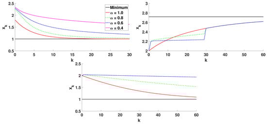
Figure 1. Algorithm 1 for different orders of differentiation, $\alpha$.

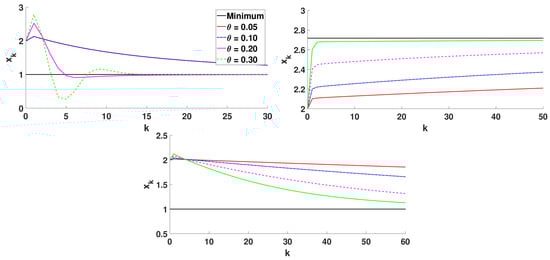
Figure 2. Algorithm 1 for different step sizes, $\theta$.

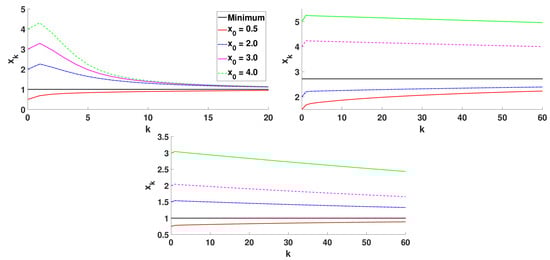
Figure 3. Algorithm 1 for different initial approximations, $x_0$.

Analyzing the plots in Figure 1, we see that the convergence of the $\psi$-FGM in the non-integer case is slower, in general, than in the integer case ($\alpha =1.0$). In Figure 2, we consider $x_0=2$, $\alpha =0.75$, $ϵ={10}^{-9}$, and different step sizes $\theta =0.05,0.1,0.2,0.3$.

The plots in Figure 2 show that the increment of the step size makes convergence faster. The optimization of the step size in each iteration would lead to the optimal convergence of the method in a few iterations. In Figure 3, we consider different initial approximations $x_0$, and the values $\alpha =0.75$, $\theta =0.1$, and $ϵ={10}^{-9}$. As expected, convergence becomes faster as $x_0$ approaches the minimum point.

Now, we show the numerical simulations of Algorithm 1 with a variable order of differentiation $\alpha \left(x\right)$. In Figure 4, we consider $\theta =0.1$, $\beta =0.1$, $x_0=2$, $ϵ={10}^{-9}$, and the variable order Functions (54)–(58). In Figure 5, we exhibit the behaviour of the algorithm for $\alpha \left(x\right)$ given by (58) and different values of $\beta$.

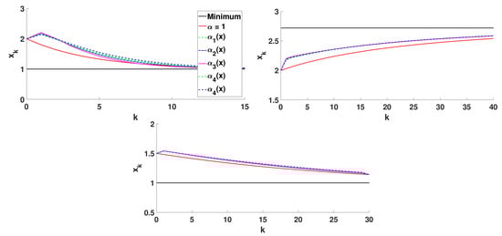
Figure 4. Algorithm 1 for different variable orders of differentiation.

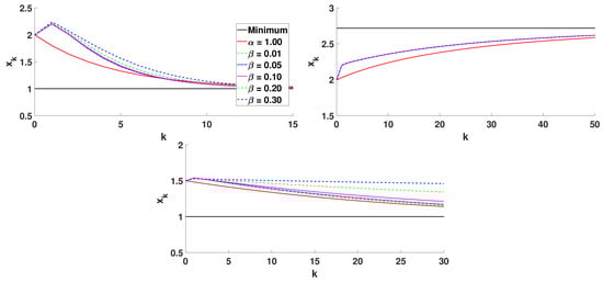
Figure 5. Algorithm 1 with $\alpha \left(x\right)=1-tanh\left(\beta J\right(x\left)\right)$ and different values of $\beta$.

From these plots, we conclude that in the one-dimensional case, the consideration of variable order differentiation can speed up the convergence, but it is, in general, slower than the classical gradient descent method with integer derivative. A further improvement of the algorithm could be made by considering a variable step size optimized in each iteration. This idea is implemented in the next section, where we consider optimization problems in ${\mathbb{R}}^2$.

5.2. The Two-Dimensional Case

5.2.1. Untrained Approach

Motivated by the ideas presented in [14,15], we extend the results presented in Section 5.1 to the two-dimensional case. We consider a function $\psi$ in the conditions of Definition 2 and the vector-valued function $\Psi :{\mathbb{R}}^2\to {\mathbb{R}}^2$ given by $\Psi \left(X\right)=\left(\psi \left(x\right),\psi \left(y\right)\right)$ with $X=\left(x,y\right)$. Moreover, let $f:{\mathbb{R}}^2\to \mathbb{R}$ be a function that admits a local minimum at the point $X^{*}$ in ${\mathbb{D}}_{\rho }\left(X^{*}\right)=\left\{X\in {\mathbb{R}}^2:∥X-X^{*}∥<\rho \right\}$ for some $\rho >0$. We want to find a local minimum point of the function $f\left(\Psi \left(X\right)\right)=f\left(\psi \left(x\right),\psi \left(y\right)\right)$, with $X=\left(x,y\right)$, through the iterative method

$$\begin{array}{c}\hfill X_{k+1}=X_k-\theta \left({{}^H\nabla }_{X_{k-1}^{+}}^{\alpha ,\mu ;\psi }f\right)\left(\Psi \left(X_k\right)\right),\theta >0.\end{array}$$

(60)

We assume that f admits a Taylor series centered at the point $\left(a_1,a_2\right)\in {\mathbb{D}}_{\rho }\left(X^{*}\right)$, given by

$$\begin{array}{c}\hfill f\left(x,y\right)=\sum _{p=0}^{+\infty }\sum _{q=0}^{+\infty }\left(\frac{{\partial }^{p+q}f}{{\partial }_x^p{\partial }_y^q}\right)\left(a_1,a_2\right)\frac{1}{p!q!}{\left(x-a_1\right)}^p{\left(y-a_2\right)}^q,\end{array}$$

(61)

with a domain of convergence $D\subseteq {\mathbb{R}}^2$, such that $X^{*}\in D.$ Then, the $\psi$-Hilfer fractional gradient in (60) is given by

$$\begin{array}{c}\hfill \left({{}^H\nabla }_{X_{k-1}^{+}}^{\alpha ,\mu ;\psi }f\right)\left(\Psi \left(X_k\right)\right)=\left(\left({{}_{x_{k-1}^{+}}{}^H\partial }_x^{\alpha ,\mu ;\psi }f\right)\left(\Psi \left(X_k\right)\right),\left({{}_{y_{k-1}^{+}}{}^H\partial }_y^{\alpha ,\mu ;\psi }f\right)\left(\Psi \left(X_k\right)\right)\right),\end{array}$$

(62)

where $\left({{}_{x_{k-1}^{+}}{}^H\partial }_x^{\alpha ,\mu ;\psi }f\right)\left(\Psi \left(X_k\right)\right)$ and $\left({{}_{y_{k-1}^{+}}{}^H\partial }_x^{\alpha ,\mu ;\psi }f\right)\left(\Psi \left(X_k\right)\right)$ denote the partial $\psi$-Hilfer derivatives of f, with respect to x and y, of order $\alpha \in [0,1]$, type $\mu \in [0,1]$, and with the lower limit of integration replaced by $x_{k-1}$ and $y_{k-1},$ respectively. Taking into account (61) and (5), we have the following expressions for the components of (62)

$$\begin{array}{c}\left({{}_{x_{k-1}^{+}}{}^H\partial }_x^{\alpha ,\mu ;\psi }f\right)\left(\Psi \left(X_k\right)\right)\hfill \\ ={\displaystyle \sum _{p=p_0}^{+\infty }}{\displaystyle \sum _{q=0}^{+\infty }}\left(\frac{{\partial }^{p+q}f}{{\partial }_x^p{\partial }_y^q}\right)\left(\Psi \left(X_{k-1}\right)\right)\frac{{\left(\psi \left(y_k\right)-\psi \left(y_{k-1}\right)\right)}^q}{q!}\frac{{\left(\psi \left(x_k\right)-\psi \left(x_{k-1}\right)\right)}^{p-\alpha }}{\Gamma \left(p+1-\alpha \right)},\hfill \end{array}$$

(63)

$$\begin{array}{c}\left({{}_{y_{k-1}^{+}}{}^H\partial }_x^{\alpha ,\mu ;\psi }f\right)\left(\Psi \left(X_k\right)\right)\hfill \\ =\sum _{p=0}^{+\infty }\sum _{q=q_0}^{+\infty }\left(\frac{{\partial }^{p+q}f}{{\partial }_x^p{\partial }_y^q}\right)\left(\Psi \left(X_{k-1}\right)\right)\frac{{\left(\psi \left(x_k\right)-\psi \left(x_{k-1}\right)\right)}^p}{p!}\frac{{\left(\psi \left(y_k\right)-\psi \left(y_{k-1}\right)\right)}^{q-\alpha }}{\Gamma \left(q+1-\alpha \right)},\hfill \end{array}$$

(64)

where

$$\begin{array}{c}\hfill p_0=q_0=\left\{\begin{array}{cc}0,\hfill & \mathrm{if}\mu \in [0,1]\hfill \\ 1,\hfill & \mathrm{if}\mu =1\hfill \end{array}\right..\end{array}$$

(65)

The iterative method proposed in (60) takes into account the short memory characteristics of the fractional derivatives and, as in the one-dimensional case, we can see from (63) and (64) that the method does not depend on the type of derivative $\mu$. Furthermore, due to the freedom of choice of the $\mu$ parameter ($\mu =1$ or $\mu \in [0,1]$) and the $\psi$ function, we can deal with several fractional derivatives (see Section 5 in [19]). We obtain the following convergence results:

Theorem 8.

If the algorithm (60) is convergent where the fractional gradient is given by (62)–(64), then it converges to the minimum point of $f\left(\Psi \left(·\right)\right)$.

Proof. 

Let $X^{*}$ be the minimum point of $f\left(\Psi \left(·\right)\right)$. We prove that the sequence ${\left(X_k\right)}_{k\in \mathbb{N}}$ converges to $X^{*}$ by contradiction. Assume that $X_k$ converges to a different $X\ne X^{*}$ and $f_x^{\prime }\left(\Psi \left(X\right)\right)\ne 0\ne f_y^{\prime }\left(\Psi \left(X\right)\right)$. As the algorithm is convergent, we have that ${lim}_{k\to +\infty }∥X_k-X∥=0$. Moreover, for any small positive $ϵ$, there exists a sufficiently large number $N\in \mathbb{N}$, such that

$$\begin{array}{c}\hfill {\left(\psi \left(x_{k-1}\right)-\psi \left(x\right)\right)}^2<\frac{{ϵ}^2}{2}<{\left(\psi \left(x^{*}\right)-\psi \left(x\right)\right)}^2\end{array}$$

(66)

and

$$\begin{array}{c}\hfill {\left(\psi \left(y_{k-1}\right)-\psi \left(y\right)\right)}^2<\frac{{ϵ}^2}{2}<{\left(\psi \left(y^{*}\right)-\psi \left(y\right)\right)}^2\end{array}$$

(67)

for any $k>N$. Thus,

$$\begin{array}{c}\hfill {\delta }_1=\underset{p,q>N}{inf}\left|\frac{{\partial }^{p_0}f}{\partial x^{p_0}}(\Psi \left(X_{k-1}\right))\right|>0\mathrm{and}{\delta }_2=\underset{p,q>N}{inf}\left|\frac{{\partial }^{q_0}f}{\partial y^{q_0}}(\Psi \left(X_{k-1}\right))\right|>0\end{array}$$

(68)

must hold. From (62)–(64) we have

$$\begin{array}{cc}\hfill & {∥X_{k+1}-X_k∥}^2\hfill \\ \hfill & ={\theta }^2{∥{{}^H\nabla }_{x_{k-1}^{+}}^{\alpha ,\mu ;\psi }f\left(\Psi \left(X_{k-1}\right)\right)∥}^2\hfill \\ \hfill & ={\theta }^2{\left(\sum _{p=0}^{+\infty }\sum _{q=0}^{+\infty }\left(\frac{{\partial }^{p+p_0+q}f}{{\partial }_x^{p+p_0}{\partial }_y^q}\right)\left(\Psi \left(X_{k-1}\right)\right)\frac{{\left(\psi \left(y_k\right)-\psi \left(y_{k-1}\right)\right)}^q}{q!}\frac{{\left(\psi \left(x_k\right)-\psi \left(x_{k-1}\right)\right)}^{p+p_0-\alpha }}{\Gamma \left(p+p_0+1-\alpha \right)}\right)}^2\hfill \\ \hfill & +{\theta }^2{\left(\sum _{p=0}^{+\infty }\sum _{q=0}^{+\infty }\left(\frac{{\partial }^{p+q+q_0}f}{{\partial }_x^p{\partial }_y^{q+q_0}}\right)\left(\Psi \left(X_{k-1}\right)\right)\frac{{\left(\psi \left(x_k\right)-\psi \left(x_{k-1}\right)\right)}^p}{p!}\frac{{\left(\psi \left(y_k\right)-\psi \left(y_{k-1}\right)\right)}^{q+q_0-\alpha }}{\Gamma \left(q+q_0+1-\alpha \right)}\right)}^2\hfill \\ \hfill & \ge {\theta }^2{\left(\frac{{\partial }^{p_0}f}{\partial x^{p_0}}(\Psi \left(X_{k-1}\right))\frac{{\left(\psi \left(x_k\right)-\psi \left(x_{k-1}\right)\right)}^{p_0-\alpha }}{\Gamma \left(p_0+1-\alpha \right)}\right)}^2\hfill \\ \hfill & -{\theta }^2{\left(\sum _{p=1}^{+\infty }\sum _{q=1}^{+\infty }\left(\frac{{\partial }^{p+p_0+q}f}{{\partial }_x^p{\partial }_y^q}\right)\left(\Psi \left(X_{k-1}\right)\right)\frac{{\left(\psi \left(y_k\right)-\psi \left(y_{k-1}\right)\right)}^q}{q!}\frac{{\left(\psi \left(x_k\right)-\psi \left(x_{k-1}\right)\right)}^{p+p_0-\alpha }}{\Gamma \left(p+p_0+1-\alpha \right)}\right)}^2\hfill \\ \hfill & +{\theta }^2{\left(\frac{{\partial }^{q_0}f}{\partial y^{q_0}}(\Psi \left(X_{k-1}\right))\frac{{\left(\psi \left(y_k\right)-\psi \left(y_{k-1}\right)\right)}^{q_0-\alpha }}{\Gamma \left(q_0+1-\alpha \right)}\right)}^2\hfill \\ \hfill & -{\theta }^2{\left(\sum _{p=1}^{+\infty }\sum _{q=1}^{+\infty }\left(\frac{{\partial }^{p+q+q_0}f}{{\partial }_x^p{\partial }_y^q}\right)\left(\Psi \left(X_{k-1}\right)\right)\frac{{\left(\psi \left(x_k\right)-\psi \left(x_{k-1}\right)\right)}^p}{p!}\frac{{\left(\psi \left(y_k\right)-\psi \left(y_{k-1}\right)\right)}^{q+q_0-\alpha }}{\Gamma \left(q+q_0+1-\alpha \right)}\right)}^2.\hfill \end{array}$$

Considering

$$\begin{array}{c}\hfill C_1=\underset{p,q\ge N}{sup}\frac{\left|\frac{{\partial }^{p_0}f}{\partial x^{p_0}}(\Psi \left(X_{k-1}\right))\right|}{\Gamma \left(p_0+1-\alpha \right)q!}\mathrm{and}{C}_2=\underset{p,q\ge N}{sup}\frac{\left|\frac{{\partial }^{q_0}f}{\partial y^{q_0}}(\Psi \left(X_{k-1}\right))\right|}{\Gamma \left(q_0+1-\alpha \right)p!},\end{array}$$

from the previous expression, we obtain

$$\begin{array}{cc}\hfill {∥X_{k+1}-X_k∥}^2& \ge {\theta }^2{\left(\frac{{\partial }^{p_0}f}{\partial x^{p_0}}(\Psi \left(X_{k-1}\right))\frac{{\left(\psi \left(x_k\right)-\psi \left(x_{k-1}\right)\right)}^{p_0-\alpha }}{\Gamma \left(p_0+1-\alpha \right)}\right)}^2\hfill \\ \hfill & -{\theta }^2{C}_1^2{\left(\sum _{p=1}^{+\infty }\sum _{q=1}^{+\infty }{\left(\psi \left(y_k\right)-\psi \left(y_{k-1}\right)\right)}^q{\left(\psi \left(x_k\right)-\psi \left(x_{k-1}\right)\right)}^{p+p_0-\alpha }\right)}^2\hfill \\ \hfill & +{\theta }^2{\left(\frac{{\partial }^{q_0}f}{\partial y^{q_0}}(\Psi \left(X_{k-1}\right))\frac{{\left(\psi \left(y_k\right)-\psi \left(y_{k-1}\right)\right)}^{q_0-\alpha }}{\Gamma \left(q_0+1-\alpha \right)}\right)}^2\hfill \\ \hfill & -{\theta }^2{C}_2^2{\left(\sum _{p=1}^{+\infty }\sum _{q=1}^{+\infty }{\left(\psi \left(x_k\right)-\psi \left(x_{k-1}\right)\right)}^p{\left(\psi \left(y_k\right)-\psi \left(y_{k-1}\right)\right)}^{q+q_0-\alpha }\right)}^2.\hfill \end{array}$$

The double series that appears in the previous expression are of a geometric type with positive radius less than 1. Hence, by the sum of a geometric series, we have

$$\begin{array}{cc}\hfill {∥X_{k+1}-X_k∥}^2& \ge {\theta }^2{\left(\frac{{\partial }^{p_0}f}{\partial x^{p_0}}(\Psi \left(X_{k-1}\right))\frac{{\left(\psi \left(x_k\right)-\psi \left(x_{k-1}\right)\right)}^{p_0-\alpha }}{\Gamma \left(p_0+1-\alpha \right)}\right)}^2\hfill \\ \hfill & -{\theta }^2{C}_1^2{\left(\frac{\psi \left(y_k\right)-\psi \left(y_{k-1}\right)}{1-\left(\psi \left(y_k\right)-\psi \left(y_{k-1}\right)\right)}\right)}^2{\left(\frac{{\left(\psi \left(x_k\right)-\psi \left(x_{k-1}\right)\right)}^{1+p_0-\alpha }}{1-\left(\psi \left(x_k\right)-\psi \left(x_{k-1}\right)\right)}\right)}^2\hfill \\ \hfill & +{\theta }^2{\left(\frac{{\partial }^{q_0}f}{\partial y^{q_0}}(\Psi \left(X_{k-1}\right))\frac{{\left(\psi \left(y_k\right)-\psi \left(y_{k-1}\right)\right)}^{q_0-\alpha }}{\Gamma \left(q_0+1-\alpha \right)}\right)}^2\hfill \\ \hfill & -{\theta }^2{C}_2^2{\left(\frac{\psi \left(x_k\right)-\psi \left(x_{k-1}\right)}{1-\left(\psi \left(x_k\right)-\psi \left(x_{k-1}\right)\right)}\right)}^2{\left(\frac{{\left(\psi \left(y_k\right)-\psi \left(y_{k-1}\right)\right)}^{1+q_0-\alpha }}{1-\left(\psi \left(y_k\right)-\psi \left(y_{k-1}\right)\right)}\right)}^2,\hfill \end{array}$$

which is equivalent to

$$\begin{array}{cc}\hfill & {∥X_{k+1}-X_k∥}^2\hfill \\ \hfill & \ge {\theta }^2\left({\left(\frac{\frac{{\partial }^{p_0}f}{\partial x^{p_0}}(\Psi \left(X_{k-1}\right))}{\Gamma \left(p_0+1-\alpha \right)}\right)}^2-C_1^2{\left(\frac{\psi \left(y_k\right)-\psi \left(y_{k-1}\right)}{1-\left(\psi \left(y_k\right)-\psi \left(y_{k-1}\right)\right)}\right)}^2{\left(\frac{\psi \left(x_k\right)-\psi \left(x_{k-1}\right)}{1-\left(\psi \left(x_k\right)-\psi \left(x_{k-1}\right)\right)}\right)}^2\right)\hfill \\ \hfill & \times {\left({\left(\psi \left(x_k\right)-\psi \left(x_{k-1}\right)\right)}^{p_0-\alpha }\right)}^2\hfill \end{array}$$

$$\begin{array}{cc}\hfill & +{\theta }^2\left({\left(\frac{\frac{{\partial }^{q_0}f}{\partial y^{q_0}}(\Psi \left(X_{k-1}\right))}{\Gamma \left(q_0+1-\alpha \right)}\right)}^2-C_2^2{\left(\frac{\psi \left(x_k\right)-\psi \left(x_{k-1}\right)}{1-\left(\psi \left(x_k\right)-\psi \left(x_{k-1}\right)\right)}\right)}^2{\left(\frac{\psi \left(y_k\right)-\psi \left(y_{k-1}\right)}{1-\left(\psi \left(y_k\right)-\psi \left(y_{k-1}\right)\right)}\right)}^2\right)\hfill \\ \hfill & \times {\left({\left(\psi \left(y_k\right)-\psi \left(y_{k-1}\right)\right)}^{q_0-\alpha }\right)}^2\hfill \\ \hfill & \ge d_1{\left({\left(\psi \left(x_k\right)-\psi \left(x_{k-1}\right)\right)}^{p_0-\alpha }\right)}^2+d_2{\left({\left(\psi \left(y_k\right)-\psi \left(y_{k-1}\right)\right)}^{q_0-\alpha }\right)}^2,\hfill \end{array}$$

(69)

where

$$\begin{array}{c}\hfill d_1=d_1\left(ϵ\right)={\theta }^2\left({\left(\frac{{\delta }_1}{\Gamma \left(p_0+1-\alpha \right)}\right)}^2-C_1^2{\left(\frac{ϵ}{1-ϵ}\right)}^4\right)\end{array}$$

and

$$\begin{array}{c}\hfill d_2=d_2\left(ϵ\right)={\theta }^2\left({\left(\frac{{\delta }_2}{\Gamma \left(q_0+1-\alpha \right)}\right)}^2-C_2^2{\left(\frac{ϵ}{1-ϵ}\right)}^4\right).\end{array}$$

One can always find $ϵ$ sufficiently small, such that

$$\begin{array}{cc}\hfill & {\left(\frac{{\delta }_1}{\Gamma \left(p_0+1-\alpha \right)}\right)}^2-C_1^2{\left(\frac{ϵ}{1-ϵ}\right)}^4>\frac{{ϵ}^{2\alpha }}{{\theta }^2}\hfill \\ \hfill & \iff {\left(\frac{{\delta }_1}{\Gamma \left(p_0+1-\alpha \right)}\right)}^2>\frac{{ϵ}^{2\alpha }}{{\theta }^2}+C_1^2{\left(\frac{ϵ}{1-ϵ}\right)}^4\hfill \end{array}$$

(70)

and

$$\begin{array}{cc}\hfill & {\left(\frac{{\delta }_2}{\Gamma \left(q_0+1-\alpha \right)}\right)}^2-C_1^2{\left(\frac{ϵ}{1-ϵ}\right)}^4>\frac{{ϵ}^{2\alpha }}{{\theta }^2}\hfill \\ \hfill & \iff {\left(\frac{{\delta }_2}{\Gamma \left(q_0+1-\alpha \right)}\right)}^2>\frac{{ϵ}^{2\alpha }}{{\theta }^2}+C_2^2{\left(\frac{ϵ}{1-ϵ}\right)}^4,\hfill \end{array}$$

(71)

because the functions

$$\begin{array}{c}\hfill g_1\left(ϵ\right)=\frac{{ϵ}^{2\alpha }}{{\theta }^2}+C_1^2{\left(\frac{ϵ}{1-ϵ}\right)}^4\mathrm{and}{g}_2\left(ϵ\right)=\frac{{ϵ}^{2\alpha }}{{\theta }^2}+C_2^2{\left(\frac{ϵ}{1-ϵ}\right)}^4\end{array}$$

are positive increasing for $\alpha \in [0,1]$, $\theta \in [0,1]$, and $ϵ\in [0,1]$. Hence, from (69) and taking into account (70) and (71), we obtain

$$\begin{array}{c}\hfill {∥X_{k+1}-X_k∥}^2>{ϵ}^{2\alpha }{ϵ}^{2p_0-2\alpha }+{ϵ}^{2\alpha }{ϵ}^{2q_0-2\alpha }=\left\{\begin{array}{cc}2{ϵ}^2,\hfill & \mathrm{if}\mu =1\hfill \\ 2,\hfill & \mathrm{if}\mu \in [0,1]\hfill \end{array}\right..\end{array}$$

(72)

On the other hand, from assumption (71), we have

$$\begin{array}{cc}\hfill & {∥X_{k+1}-X_k∥}^2\hfill \\ \hfill & \le {∥\Psi \left(X_{k+1}\right)-\Psi \left(X_k\right)∥}^2\hfill \\ \hfill & \le {\left(\psi \left(x_{k+1}\right)-\psi \left(x_k\right)\right)}^2+{\left(\psi \left(y_{k+1}\right)-\psi \left(y_k\right)\right)}^2\hfill \\ \hfill & \le {\left(\psi \left(x_{k+1}\right)-\psi \left(x\right)\right)}^2+{\left(\psi \left(x\right)-\psi \left(x_k\right)\right)}^2+{\left(\psi \left(y_{k+1}\right)-\psi \left(y\right)\right)}^2{\left(\psi \left(y\right)-\psi \left(y_k\right)\right)}^2\hfill \end{array}$$

$$\begin{array}{cc}\hfill & <\frac{{ϵ}^2}{2}+\frac{{ϵ}^2}{2}+\frac{{ϵ}^2}{2}+\frac{{ϵ}^2}{2}=2{ϵ}^2,\hfill \end{array}$$

which contradicts (72). This completes the proof.    □

Despite the convergence of (60), it is important to point out that sometimes the function $f\left(\Psi \left(·\right)\right)$ is not smooth enough. In these cases, the algorithm involving the double series (63) and (64) cannot be implemented. Moreover, in the same way as was done for the one-dimensional case, assuming that f is at least of the class $C^1,$ we only consider the following terms of (63) and (64)

$$\begin{array}{cc}\hfill & \frac{f_x^{\prime }(\Psi \left(X_{k-1}\right))}{\Gamma \left(2-\alpha \right)}{\left(\psi \left(x_k\right)-\psi \left(x_{k-1}\right)\right)}^{1-\alpha }\left(\mathrm{term}p=1\mathrm{and}q=0\mathrm{in}\left(63\right)\right),\hfill \\ \hfill & \frac{f_y^{\prime }(\Psi \left(X_{k-1}\right))}{\Gamma \left(2-\alpha \right)}{\left(\psi \left(y_k\right)-\psi \left(y_{k-1}\right)\right)}^{1-\alpha },\left(\mathrm{term}p=0\mathrm{and}q=1\mathrm{in}\left(64\right)\right).\hfill \end{array}$$

Thus, the higher order terms are eliminated and we have the following update of (62):

$$\begin{array}{cc}\hfill & \left({{}^H\nabla }_{X_{k-1}^{+}}^{\alpha ,\mu ;\psi }f\right)\left(\Psi \left(X_k\right)\right)\hfill \\ \hfill & =\left(\frac{f_x^{\prime }(\Psi \left(X_{k-1}\right))}{\Gamma \left(2-\alpha \right)}{\left(\psi \left(x_k\right)-\psi \left(x_{k-1}\right)\right)}^{1-\alpha },\frac{f_y^{\prime }(\Psi \left(X_{k-1}\right))}{\Gamma \left(2-\alpha \right)}{\left(\psi \left(y_k\right)-\psi \left(y_{k-1}\right)\right)}^{1-\alpha }\right).\hfill \end{array}$$

To avoid the appearance of complex numbers, we also consider

$$\begin{array}{cc}\hfill & \left({{}^H\nabla }_{X_{k-1}^{+}}^{\alpha ,\mu ;\psi }f\right)\left(\Psi \left(X_k\right)\right)\hfill \\ \hfill & =\left(\frac{f_x^{\prime }(\Psi \left(X_{k-1}\right))}{\Gamma \left(2-\alpha \right)}{\left|\psi \left(x_k\right)-\psi \left(x_{k-1}\right)\right|}^{1-\alpha },\frac{f_y^{\prime }\left(\Psi \left(X_{k-1}\right)\right)}{\Gamma \left(2-\alpha \right)}{\left|\psi \left(y_k\right)-\psi \left(y_{k-1}\right)\right|}^{1-\alpha }\right).\hfill \end{array}$$

(73)

The implementation of (73) is presented in Algorithm 2. In a similar way as it was done in Theorem 8, we can state the following results.

Theorem 9.

If the algorithm (60) is convergent where the fractional gradient is given by (73), then it converges to the minimum point of $f\left(\Psi \left(·\right)\right)$.

Algorithm 2: 2D $\psi$-FGM with higher order truncation.

5.2.2. The Trained Approach

In this section, we refine Algorithm 2 in two ways that train our algorithm in each iteration to find the most accurate $X_k$. First, we consider a variable step size ${\theta }_k>0$ that is updated in each iteration by minimizing the following function

$$\begin{array}{c}\hfill \varphi \left({\theta }_k\right)=f\left(\Psi \left(X_k\right)-{\theta }_k\left({{}^H\nabla }_{X_{k-1}^{+}}^{\alpha ,\mu ;\psi }f\right)\left(\Psi \left(X_k\right)\right)\right).\end{array}$$

In the second refinement, we adjust the order of integration $\alpha$ with $X_k$. More precisely, if f is a non-negative function with a unique minimum point $X^{*}$, we can consider any of the functions (54)–(58). In our approach, we only consider the following variable fractional order

$$\begin{array}{c}\hfill \alpha \left(X\right)=1-\frac{2}{\pi }arctan\left(\beta J\left(X\right)\right),\end{array}$$

(74)

where the loss function is $J\left(X\right)=∥\nabla f(\Psi \left(X\right))∥$. From (74), we infer that when $J\left(X\right)\approx 0$, one has $\alpha \left(X\right)\approx 1$, and when $J\left(X\right)\gg 0$, one has $\alpha \left(X\right)\approx 0$. As a consequence of the previous refinements, we have the following iterative method:

$$\begin{array}{c}\hfill X_{k+1}=X_k-{\theta }_k\left({{}^H\nabla }_{X_{k-1}^{+}}^{\alpha \left(X_k\right),\mu ;\psi }f\right)\left(\Psi \left(X_k\right)\right),\end{array}$$

(75)

where the fractional gradient is given by

$$\begin{array}{cc}\hfill & \left({{}^H\nabla }_{X_{k-1}^{+}}^{\alpha \left(X_k\right),\mu ;\psi }f\right)\left(\Psi \left(X_k\right)\right)\hfill \\ \hfill & =\left(\frac{f_x^{\prime }(\Psi \left(X_{k-1}\right))}{\Gamma \left(2-\alpha \left(X_k\right)\right)}{\left|\psi \left(x_k\right)-\psi \left(x_{k-1}\right)\right|}^{1-\alpha \left(X_k\right)},\frac{f_y^{\prime }(\Psi \left(X_{k-1}\right))}{\Gamma \left(2-\alpha \left(X_k\right)\right)}{\left|\psi \left(y_k\right)-\psi \left(y_{k-1}\right)\right|}^{1-\alpha \left(X_k\right)}\right).\hfill \end{array}$$

(76)

The implementation of (76) is presented in Algorithm 3. Likewise, with a variable fractional order $\alpha \left(X\right)$, the following theorem follows.

Theorem 10.

If the algorithm (75) is convergent where the fractional gradient is given by (76), then it converges to the minimum point of $f\left(\Psi \left(·\right)\right)$.

The proof of this result follows the same reasoning of the proof of Theorem 8, and therefore, is omitted.

Algorithm 3: 2D $\psi$-FGM with variable fractional order and optimized step size.

5.2.3. Numerical Simulations

In this section, we implement Algorithms 2 and 3 for finding the local minimum point of the function $f\left(\Psi \left(·\right)\right)$ for particular choices of f and $\psi$. For the function f, we consider the following cases:

• $f_1\left(x,y\right)=4x^2-4xy+2y^2$ with minimum point at $\left(0,0\right)$,
• Matyas function: $f_2\left(x,y\right)=0.26\left(x^2+y^2\right)-0.48xy$ with minimum point at $\left(0,0\right)$,
• Wayburn and Seader No. 1 function: $f_3\left(x,y\right)={\left(x^6+y^4-17\right)}^2+{\left(2x+y-4\right)}^2$ with minimum point at $\left(1,2\right)$.

The function $f_1$ is a classic convex quadratic function in ${\mathbb{R}}^2$ and can be considered an academic example for implementing our algorithms. The choice of functions $f_2$ and $f_3$ is due to the fact that they are benchmark functions used to test and evaluate several characteristics of optimization algorithms, such as convergence rate, precision, robustness, and general performance. More precisely, the Matyas function has a plate shape and the Wayburn and Seader No. 1 function has a valley shape, which implies slow convergence to the minimum point of the corresponding function. For the functions $\psi$ in the vector function $\Psi ,$ we consider the choices

• ${\psi }_1\left(x\right)=x$, with $x\in I=[0,+\infty [$,
• ${\psi }_2\left(x\right)=x^2$, with $x\in I=[0,+\infty [$,
• ${\psi }_3\left(x\right)=lnx,$ with $x\in I=[1,+\infty [$.

For the numerical simulations, we consider some combinations of the functions $f_i$, $i=1,2$, and ${\psi }_j$, $j=1,2,3$, and compare the results in the following scenarios:

• Algorithm 3 with $\alpha \left(X\right)=1$ that corresponds to the classical 2D gradient descent method,
• Algorithm 2 with $\alpha \left(X\right)=0.8$ and step size $\theta =0.1$,
• Algorithm 3 with $\alpha \left(X\right)=1-{\displaystyle \frac{2}{\pi }}arctan\left(\beta J\left(X\right)\right),$ with $\beta =0.1$.

Figure 6 shows the target functions $f_1\left({\Psi }_1\left(X\right)\right)=4x^2-4xy+2y^2$ and $f_1\left({\Psi }_2\left(X\right)\right)=4x^4-4x^2{y}^2+2y^4$, both with a local minimum point at $X^{*}=\left(0,0\right)$. Figure 7 and Figure 8 show the $X_k$ iterates in the corresponding contour plots of the functions. The plots on the right show the amplification close to the minimum point. The results of numerical simulations are summarized in Table 1. The stopping criterion used was $ϵ={10}^{-9}$.

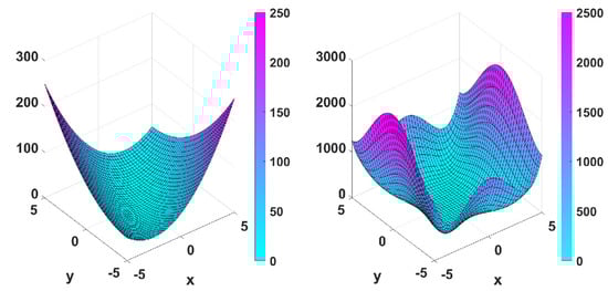
Figure 6. Graphical representations of $f_1\left({\Psi }_1\left(X\right)\right)$ and $f_1\left({\Psi }_2\left(X\right)\right)$.

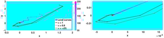
Figure 7. Iterates for $f_1\left({\Psi }_1\left(X\right)\right)$.

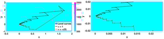
Figure 8. Iterates for $f_1\left({\Psi }_2\left(X\right)\right)$.

Table 1. Information about the k-iteration associated with Figure 7 and Figure 8.

	$\mathit{\alpha }$	$\mathit{\theta }$	k	${\mathit{X}}_0$	${\mathit{X}}_{\mathit{k}}$	$∥{\mathit{X}}_{\mathit{k}}-{\mathit{X}}^{*}∥$
	$f_1\left({\Psi }_1\left(X\right)\right)$
Classical Gradient	1.0	optimized	49	$\left[1.50,2.50\right]$	$\left[7.8188\times {10}^{-11},1.3031\times {10}^{-10}\right]$	$1.5197\times {10}^{10}$
Algorithm 2	0.8	0.1	2480	$\left[0.75,1.25\right]$	$\left[3.3860\times {10}^{-8},5.3902\times {10}^{-8}\right]$	$6.3655\times {10}^{-10}$
Algorithm 3	variable	optimized	50	$\left[1.50,2.50\right]$	$\left[9.3483\times {10}^{-11},1.4213\times {10}^{-10}\right]$	$1.7012\times {10}^{-10}$
	$f_1\left({\Psi }_2\left(X\right)\right)$
Classical Gradient	1.0	optimized	77	$\left[1.50,2.50\right]$	$\left[3.3370\times {10}^{-4},5.5617\times {10}^{-4}\right]$	$6.4860\times {10}^{-4}$
Algorithm 2	0.8	0.1	divergence	$\left[0.75,1.25\right]$	—	—
Algorithm 3	variable	optimized	73	$\left[1.50,2.50\right]$	$\left[3.9399\times {10}^{-4},-5.4845\times {10}^{-4}\right]$	$6.7530\times {10}^{-4}$

In Table 1, we present the information concerning the $X_k$ iterates of the implemented algorithms. When we consider ${\Psi }_1$, we achieve the global minimum point in the three cases; however, it is clear that Algorithm 2 leads to the worst results in terms of speediness, whereas the classical case and Algorithm 3 have similar results. If we consider ${\Psi }_2$ and we restrict our analysis to the two fastest algorithms, we conclude that, in this case, Algorithm 3 provides a more accurate approximation in fewer iterations. We point out that the objective function $f_1\left({\Psi }_2\left(·\right)\right)$ is a function with less convexity near the minimum point when compared with the objective function $f_1\left({\Psi }_1\left(·\right)\right)$, which leads to an optimization problem that is more challenging under the numerical point of view.

In the next set of figures and tables, we consider the Matyas function to test our algorithms. More precisely, we consider the functions $f_2\left({\Psi }_1\left(X\right)\right)=0.26\left(x^2+y^2\right)-0.48xy$ with local minimum at the point $X^{*}=\left(0,0\right)$, and $f_2\left({\Psi }_3\left(X\right)\right)=0.26\left({ln}^2\left(x\right)+{ln}^2\left(y\right)\right)-0.48ln\left(x\right)ln\left(y\right)$ with local minimum at the point $X^{*}=\left(1,1\right)$.

Figure 9 shows both functions $f_2\left({\Psi }_1\left(·\right)\right)$ and $f_2\left({\Psi }_3\left(·\right)\right)$ with a plate-like shape. Considering the same stopping criteria, we have the following results.

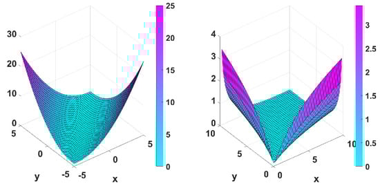
Figure 9. Graphical representations of $f_2\left({\Psi }_1\left(X\right)\right)$ and $f_2\left({\Psi }_3\left(X\right)\right)$.

From the analysis of Table 2, we see that the three methods converge in the case of $f_2\left({\Psi }_1\right)$, but Algorithm 2 is the worst in terms of iterations. The classic case and Algorithm 3 have similar results in terms of precision; however, Algorithm 3 presents better performance in terms of the number of iterations. In the case of $f_2\left({\Psi }_3\right)$, the Algorithm 2 diverges and the other two are convergent. Algorithm 3 required half of the iterations compared with the classical gradient method.

Table 2. Information about the k-iteration associated with Figure 10 and Figure 11.

	$\mathit{\alpha }$	$\mathit{\theta }$	k	${\mathit{X}}_0$	${\mathit{X}}_{\mathit{k}}$	$∥{\mathit{X}}_{\mathit{k}}-{\mathit{X}}^{*}∥$
	$f_2\left({\Psi }_1\left(X\right)\right)$
Classical Gradient	1.0	optimized	43	$\left[1.50,2.50\right]$	$\left[8.9458\times {10}^{-9},8.8320\times {10}^{-9}\right]$	$1.2571\times {10}^{-8}$
Algorithm 2	0.8	1.0	94777	$\left[0.75,1.25\right]$	$\left[1.7395\times {10}^{-6},1.7395\times {10}^{-6}\right]$	$2.4600\times {10}^{-6}$
Algorithm 3	variable	optimized	27	$\left[1.50,2.50\right]$	$\left[1.4056\times {10}^{-8},1.3811\times {10}^{-8}\right]$	$1.9727\times {10}^{-8}$
	$f_2\left({\Psi }_3\left(X\right)\right)$
Classical Gradient	1.0	optimized	51	$\left[1.50,2.50\right]$	$\left[1,1\right]$	$0.5\times {10}^{-16}$
Algorithm 2	0.8	0.1	divergence	$\left[0.75,1.25\right]$	—	—
Algorithm 3	variable	optimized	29	$\left[1.50,2.50\right]$	$\left[1,1\right]$	$0.5\times {10}^{-6}$

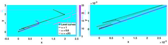
Figure 10. Iterates for $f_2\left({\Psi }_1\left(X\right)\right)$.

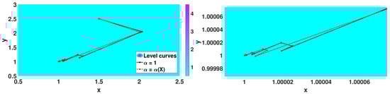
Figure 11. Iterates for $f_2\left({\Psi }_3\left(X\right)\right)$.

Table 2. Information about the k-iteration associated with Figure 10 and Figure 11.

	$\mathit{\alpha }$	$\mathit{\theta }$	k	${\mathit{X}}_0$	${\mathit{X}}_{\mathit{k}}$	$∥{\mathit{X}}_{\mathit{k}}-{\mathit{X}}^{*}∥$
	$f_2\left({\Psi }_1\left(X\right)\right)$
Classical Gradient	1.0	optimized	43	$\left[1.50,2.50\right]$	$\left[8.9458\times {10}^{-9},8.8320\times {10}^{-9}\right]$	$1.2571\times {10}^{-8}$
Algorithm 2	0.8	1.0	94777	$\left[0.75,1.25\right]$	$\left[1.7395\times {10}^{-6},1.7395\times {10}^{-6}\right]$	$2.4600\times {10}^{-6}$
Algorithm 3	variable	optimized	27	$\left[1.50,2.50\right]$	$\left[1.4056\times {10}^{-8},1.3811\times {10}^{-8}\right]$	$1.9727\times {10}^{-8}$
	$f_2\left({\Psi }_3\left(X\right)\right)$
Classical Gradient	1.0	optimized	51	$\left[1.50,2.50\right]$	$\left[1,1\right]$	$0.5\times {10}^{-16}$
Algorithm 2	0.8	0.1	divergence	$\left[0.75,1.25\right]$	—	—
Algorithm 3	variable	optimized	29	$\left[1.50,2.50\right]$	$\left[1,1\right]$	$0.5\times {10}^{-6}$

In the final set of figures and tables, the function $f_3$ is composed with ${\Psi }_1$ and ${\Psi }_2$. Taking into account the results obtained previously for the Matyas function, where it is clear that Algorithm 2 leads to worse results in terms of rapidness and accuracy, we only implemented the classical gradient method and Algorithm 3. The following figure shows the graphical representation of $f_3\left({\Psi }_1\left(X\right)\right)={\left(x^6+y^4-17\right)}^2+{\left(2x+y-4\right)}^2$ with local minimum at the point $X^{*}=\left(1,2\right)$ and $f_3\left({\Psi }_2\left(X\right)\right)={\left(x^{12}+y^8-17\right)}^2+{\left(2x^2+y^2-4\right)}^2$ with local maximum at $X^{*}=\left(0,0\right)$ (or a local minimum of the function $-f_3\left({\Psi }_2\left(X\right)\right)$).

The plots in Figure 12 show that both functions are valley-shaped. Figure 13 and Figure 14 and Table 3 show the obtained numerical results.

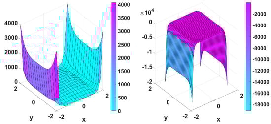
Figure 12. Graphical representations of $f_3\left({\Psi }_1\left(X\right)\right)$ and $-f_3\left({\Psi }_2\left(X\right)\right)$.

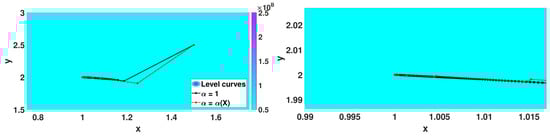
Figure 13. Iterates for $f_3\left({\Psi }_1\left(X\right)\right)$.

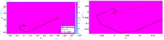
Figure 14. Iterates for $f_3\left({\Psi }_2\left(X\right)\right)$.

Table 3. Information about the k-iteration associated with Figure 13 and Figure 14.

	$\mathit{\alpha }$	$\mathit{\theta }$	k	${\mathit{X}}_0$	${\mathit{X}}_{\mathit{k}}$	$∥{\mathit{X}}_{\mathit{k}}-{\mathit{X}}^{*}∥$
	$f_3\left({\Psi }_1\left(X\right)\right)$
Classical Gradient	1.0	optimized	2923	$\left[1.50,2.50\right]$	$\left[1,2\right]$	$0.5\times {10}^{-16}$
Algorithm 3	variable	optimized	71	$\left[1.50,2.50\right]$	$\left[1,2\right]$	$1.378364\times {10}^{-10}$
	$f_3\left({\Psi }_2\left(X\right)\right)$
Classical Gradient	1.0	optimized	51	$\left[0.50,0.25\right]$	$\left[1.6446\times {10}^{-12},-1.3283\times {10}^{-11}\right]$	$1.3385\times {10}^{-11}$
Algorithm 3	variable	optimized	39	$\left[0.50,0.25\right]$	$\left[-1.0755\times {10}^{-12},2.1842\times {10}^{-11}\right]$	$2.1868\times {10}^{-11}$

In this last case, we see that the classic gradient method and Algorithm 3 provide very good approximations. Algorithm 3 performs better in terms of the number of iterations. For instance, in the case of $f_3\left({\Psi }_1\right)$, the number of iterations decreased around 97% in comparison with the classical gradient method.

6. Conclusions

In this work, we study the classical gradient method from the perspective of the $\psi$-Hilfer fractional derivative. In the first part of the article, we consider the continuous gradient method and perform the convergence analysis for strongly and non-strongly convex cases. The identification of functions of the Lyapunov type, together with the auxiliary results demonstrated, allowed us to establish the convergence of the generating trajectories in the case of $\psi$-Hilfer.

In the second part of the paper, we first show that the $\psi$-Hilfer FGM with the $\psi$-Hilfer gradient given as a power series can converge to a point different from the extreme point. To work out this problem, we propose an algorithm with a variable lower bound of integration, reducing the influence of long-time memory terms. By truncating the higher order terms, we obtain the $\psi$-FGM, which allows easy implementation in practice. Furthermore, we optimized the step size in each iteration and considered a variable order of differentiation to increase the precision and speed of the method. These two tunable parameters improved the performance of the method in terms of speed of convergence.

Our numerical simulations showed that the proposed FGM achieved the approximation with equal or better precision, but in much fewer iterations compared with the classical gradient method with optimized step size. We emphasize that in our 2D numerical simulations, the Matyas function and the Wayburn and Seader No. 1 functions are well-known benchmark functions used to test optimization methods. These functions have the shapes of plates and valleys, respectively, representing an extra challenge in numerical simulations.

In future works, it would be interesting to further develop this theory to see its application in the field of convolutional neural networks.

References

- Lin, J.Y.; Liao, C.W. New IIR filter-based adaptive algorithm in active noise control applications: Commutation error-introduced LMS algorithm and associated convergence assessment by a deterministic approach. Automatica 2008, 44, 2916–2922. [Google Scholar] [CrossRef]
- Pu, Y.F.; Zhou, J.L.; Zhang, Y.; Zhang, N.; Huang, G.; Siarry, P. Fractional extreme value adaptive training method: Fractional steepest descent approach. IEEE Trans. Neural Netw. Learn. Syst. 2015, 26, 653–662. [Google Scholar] [CrossRef] [PubMed]
- Ge, Z.W.; Ding, F.; Xu, L.; Alsaedi, A.; Hayat, T. Gradient-based iterative identification method for multivariate equation-error autoregressive moving average systems using the decomposition technique. J. Frankl. Inst. 2019, 356, 1658–1676. [Google Scholar] [CrossRef]
- LeCun, Y.; Bengio, Y.; Hinton, G. Deep learning. Nature 2015, 521, 436–444. [Google Scholar] [CrossRef] [PubMed]
- Wong, C.C.; Chen, C.C. A hybrid clustering and gradient descent approach for fuzzy modeling. IEEE Trans. Syst. Man Cybern. Part B Cybern. 1999, 29, 686–693. [Google Scholar] [CrossRef] [PubMed]
- Ren, Z.G.; Xu, C.; Zhou, Z.C.; Wu, Z.Z.; Chen, T.H. Boundary stabilization of a class of reaction-advection-difffusion systems via a gradient-based optimization approach. J. Frankl. Inst. 2019, 356, 173–195. [Google Scholar] [CrossRef]
- Tan, Y.; He, Z.; Tian, B. A novel generalization of modified LMS algorithm to fractional order. IEEE Signal Process. Lett. 2015, 22, 1244–1248. [Google Scholar] [CrossRef]
- Cheng, S.S.; Wei, Y.H.; Chen, Y.Q.; Li, Y.; Wang, Y. An innovative fractional order LMS based on variable initial value and gradient order. Signal Process. 2017, 133, 260–269. [Google Scholar] [CrossRef]
- Raja, M.A.Z.; Chaudhary, N.I. Two-stage fractional least mean square identification algorithm for parameter estimation of CARMA systems. Signal Process. 2015, 107, 327–339. [Google Scholar] [CrossRef]
- Shah, S.M.; Samar, R.; Khan, N.M.; Raja, M.A.Z. Design of fractional-order variants of complex LMS and NLMS algorithms for adaptive channel equalization. Nonlinear Dyn. 2017, 88, 839–858. [Google Scholar] [CrossRef]
- Viera-Martin, E.; Gómez-Aguilar, J.F.; Solís-Pérez, J.E.; Hernández-Pérez, J.A.; Escobar-Jiménez, R.F. Artificial neural networks: A practical review of applications involving fractional calculus. Eur. Phys. J. Spec. Top. 2022, 231, 2059–2095. [Google Scholar] [CrossRef] [PubMed]
- Sheng, D.; Wei, Y.; Chen, Y.; Wang, Y. Convolutional neural networks with fractional order gradient method. Neurocomputing 2020, 408, 42–50. [Google Scholar] [CrossRef]
- Wang, Y.L.; Jahanshahi, H.; Bekiros, S.; Bezzina, F.; Chu, Y.M.; Aly, A.A. Deep recurrent neural networks with finite-time terminal sliding mode control for a chaotic fractional-order financial system with market confidence. Chaos Solitons Fractals 2021, 146, 110881. [Google Scholar] [CrossRef]
- Chen, Y.Q.; Gao, Q.; Wei, Y.H.; Wang, Y. Study on fractional order gradient methods. Appl. Math. Comput. 2017, 314, 310–321. [Google Scholar] [CrossRef]
- Wei, Y.; Kang, Y.; Yin, W.; Wang, Y. Generalization of the gradient method with fractional order gradient direction. J. Frankl. Inst. 2020, 357, 2514–2532. [Google Scholar] [CrossRef]
- Samko, S.G.; Kilbas, A.A.; Marichev, O.I. Fractional Integrals and Derivatives: Theory and Applications; Gordon and Breach: New York, NY, USA, 1993. [Google Scholar]
- Kilbas, A.A.; Srivastava, H.M.; Trujillo, J.J. Theory and Applications of Fractional Differential Equations; North-Holland Mathematics Studies; Elsevier: Amsterdam, The Netherlands, 2006; Volume 204. [Google Scholar]
- Almeida, R. A Caputo fractional derivative of a function with respect to another function. Commun. Nonlinear Sci. Numer. Simul. 2017, 44, 460–481. [Google Scholar] [CrossRef]
- Sousa, J.V.C.; Oliveira, E.C. On the ψ-Hilfer derivative. Commun. Nonlinear Sci. Numer. Simulat. 2018, 60, 72–91. [Google Scholar] [CrossRef]
- Gorenflo, R.; Kilbas, A.A.; Mainardi, F.; Rogosin, S.V. Mittag-Leffler Functions, Related Topics and Applications; Springer: Berlin/Heidelberg, Germany, 2020. [Google Scholar]
- Hai, P.V.; Rosenfeld, J.A. The gradient descent method from the perspective of fractional calculus. Math. Meth. Appl. Sci. 2021, 44, 5520–5547. [Google Scholar] [CrossRef]
- Kucche, K.D.; Mali, A.D.; Sousa, J.V.C. On the nonlinear ψ-Hilfer fractional differential equations. Comput. Appl. Math. 2019, 38, 73. [Google Scholar] [CrossRef]
Disclaimer/Publisher’s Note: The statements, opinions and data contained in all publications are solely those of the individual author(s) and contributor(s) and not of MDPI and/or the editor(s). MDPI and/or the editor(s) disclaim responsibility for any injury to people or property resulting from any ideas, methods, instructions or products referred to in the content. |
© 2023 by the authors. Licensee MDPI, Basel, Switzerland. This article is an open access article distributed under the terms and conditions of the Creative Commons Attribution (CC BY) license (https://creativecommons.org/licenses/by/4.0/).