On Exact Solutions of Some Space–Time Fractional Differential Equations with M-truncated Derivative

Abstract

In this study, the extended ${\mathrm{G}}^{\prime }/\mathrm{G}$ method is used to investigate the space–time fractional Burger-like equation and the space–time-coupled Boussinesq equation with M-truncated derivative, which have an important place in fluid dynamics. This method is efficient and produces soliton solutions. A symbolic computation program called Maple was used to implement the method in a dependable and effective way. There are also a few graphs provided for the solutions. Using the suggested method to solve these equations, we have provided many new exact solutions that are distinct from those previously found. By offering insightful explanations of many nonlinear systems, the study’s findings add to the body of literature. The results revealed that the suggested method is a valuable mathematical tool and that using a symbolic computation program makes these tasks simpler, more dependable, and quicker. It is worth noting that it may be used for a wide range of nonlinear evolution problems in mathematical physics. The study’s findings may have an influence on how different physical problems are interpreted.

1. Introduction

The use of nonlinear partial differential equations (NPDEs) is crucial in many disciplines, including physics, mathematics, fluid dynamics, and engineering sciences. Owing to NPDEs, numerous real-world problems have been modeled. To find exact solutions to NPDEs, a wide variety of effective mathematical techniques have been used [1,2,3,4,5,6,7,8,9,10,11,12,13,14]. Another new area that has gained interest during the past several decades is fractional calculus. Fractional differential equations (FDEs) have made many scientific phenomena, including viscoelasticity, plasma, solid mechanics, optical fibers, signal processing, electromagnetic waves, fluid dynamics, biomedical sciences, and diffusion processes, easily solvable. By employing a variety of methods to get exact solutions of FDE, researchers have improved the attractiveness of these equations. The ${\mathrm{G}}^{\prime }/{\mathrm{G}}^2$-expansion method [15,16], ansatz and Kudryashov method [17], the improved extended tanh-coth method [18], the first integral method [19], the exp-function method [20], the F-expansion method [21], the improved subequation method [22,23], and the functional variable method [24] are a few of these methods of note.

Burger’s equation has acoustic applications and has been implemented to model turbulence and some steady-state viscous flows. Moreover, it is also used in the mathematical modeling of fluid dynamics, nonlinear acoustic gas dynamics, traffic flow, shock wave theory, and turbulence problems. In the literature, Burger’s equation is presented in a number of different ways, including coupled Boussinesq Burger equations, Burger-like equations, viscous Burger equations, and inviscid Burger equations. The fractional coupled viscous Burgers equations have recently been the subject of a number of intriguing studies [25,26]. The tanh method was employed by Bulut et al. [27] to produce several solutions to this equation. Gencoglu [28] acquired complicated answers for it via a direct algebraic method. Eskandari and Taghizadeh discussed the exact solutions of the nonlinear space–time fractional Burger-like equation using the expfunction method [29].

The first model for nonlinear, dispersive wave propagation may be thought to be the Boussinesq type equations, which describe surface water waves with a horizontal scale significantly bigger than the water depth [30]. In mathematical physics, they might be considered a crucial class of fractional differential equations. To solve Boussinesq equations analytically and numerically, many methods have recently been employed. These include the exp-function method [31], the invariant subspace method [32], and the expansion method, a recently developed technique [33]. Equations of this type are also a crucial nonlinear model that may be found in physics, hydromechanics, and optics. Additionally, it is understood that it may be utilized to characterize the actual direction of wave propagation in plasma and nonlinear waves [34,35,36,37,38]. In shallow water waves for bilayer fluid flow, coupled Boussinesq equations appear. This occurs when a ship unintentionally spills oil, causing an oil slick to float above the water slide [39].

In this study, exact solutions of the space–time fractional Burger-like equation and the space–time coupled Boussinesq equation were investigated using the extended ${\mathrm{G}}^{\prime }/\mathrm{G}$ method, which has never been discussed before. For this purpose, the recently studied M-truncated derivative in fractional derivative studies, which is different from other fractional derivatives, was used. In addition, the method mentioned has not been previously used in the solution of these equations. Therefore, we emphasize that these are novel results.

This work is broken into five sections. Section 1 outlines fractional calculations and includes a brief discussion of nonlinear partial and fractional differential equations. The Burger’s equation and the Boussinesq type equations, which form the basis of this work, are also discussed. Section 2 discusses the extended ${\mathrm{G}}^{\prime }/\mathrm{G}$ method, which is an essential way for solving the problem, as well as M-truncated derivative theory. Section 3 analyzes the use of this method to obtain exact solutions to the space–time fractional Burger-Like equation and the space–time coupled Boussinesq equation. The explanations of the graphics of the solutions and the effect of the method on the results are given in Section 4. Section 5 provides an explanation of the results.

2. The Fundamental Concepts of the M-truncated Derivative and Algorithm of the Extended G${}^{\prime }$/G Method

2.1. The Basic Concepts of the M-Truncated Derivative

Some fundamental fractional calculus principles that have been employed in this study are presented in this section. These are M-truncated derivative and its features.

Definition 1. 

Assume $h:(0,\infty )\to \mathbb{R}$. For $0<\omega <1$, the truncated M-fractional derivative of $h\left(\theta \right)$ of order ω has been defined by [40] as follows:

$${}_j{\mathcal{T}}_M^{\omega ,\delta }\left\{h\left(\theta \right)\right\}=\underset{\epsilon \to 0}{lim}\frac{h\left[\theta {}_j{\mathrm{E}}_{\delta }\left(ϵ{\theta }^{-\omega }\right)\right]-h\left(\theta \right)}{ϵ},\theta >0,$$

(1)

where ${}_j{\mathrm{E}}_{\delta }(.)$ is a truncated Mittag-Leffler function of one parameter, defined as follows:

$${}_j{\mathrm{E}}_{\delta }\left(v\right)=\sum _{i=0}^j\frac{v^i}{\mathsf{\Gamma }(\delta i+1)},\delta >0,v\in \mathbb{C}.$$

(2)

Theorem  1. 

Functions $f_1\left(\theta \right)$ and $f_2\left(\theta \right)$, which are ω-derivable with $0<\omega \le 1$ and $\delta >0$ at a point $\theta >0$, satisfy the following properties [40,41]:

• ${}_j{\mathcal{T}}_M^{\omega ,\delta }\{a_1{f}_1\left(\theta \right)+a_2{f}_2\left(\theta \right)\}=a_1{}_j{\mathcal{T}}_M^{\omega ,\delta }\left\{f_1\left(\theta \right)\right\}+a_2{}_j{\mathcal{T}}_M^{\omega ,\delta }\left\{f_2\left(\theta \right)\right\}$, $\forall a_1,a_2\in \mathbb{R}$,
• ${}_j{\mathcal{T}}_M^{\omega ,\delta }\left\{f_1\left(\theta \right)f_2\left(\theta \right)\right\}=f_2{\left(\theta \right)}_j{\mathcal{T}}_M^{\omega ,\delta }\left\{f_1\left(\theta \right)\right\}+f_1{\left(\theta \right)}_j{\mathcal{T}}_M^{\omega ,\delta }\left\{f_2\left(\theta \right)\right\}$,
• ${}_j{\mathcal{T}}_M^{\omega ,\delta }\left\{\frac{f_1\left(\theta \right)}{f_2\left(\theta \right)}\right\}=\frac{f_2{\left(\theta \right)}_j{\mathcal{T}}_M^{\omega ,\delta }\left\{f_1\left(\theta \right)\right\}-f_1{\left(\theta \right)}_j{\mathcal{T}}_M^{\omega ,\delta }\left\{f_2\left(\theta \right)\right\}}{{\left(f_2\left(\theta \right)\right)}^2}$,
• ${}_j{\mathcal{T}}_M^{\omega ,\delta }{\left(\theta \right)}^n=n{\left(\theta \right)}^{n-\omega }$, $n\in \mathbb{R}$,
• If $f_1$ is differentiable, then ${}_j{\mathcal{T}}_M^{\omega ,\delta }\left(f_1\right)\left(\theta \right)=\frac{{\theta }^{1-\omega }}{\mathsf{\Gamma }(\delta +1)}\frac{d{f}_1}{d\theta }$,
• ${}_j{\mathcal{T}}_M^{\omega ,\delta }(f_1\circ f_2)\left(\theta \right)=f_1^{\prime }{\left(f_2\left(\theta \right)\right)}_j{\mathcal{T}}_M^{\omega ,\delta }\left\{f_2\left(\theta \right)\right\}$.

2.2. Description of the Extended G${}^{\prime }$/G Method

In this section, the extended ${\mathrm{G}}^{\prime }/\mathrm{G}$ method, which is applied in [42], is briefly defined. Assume that we have the nonlinear fractional differential equation as follows:

$$F(u,{\mathcal{T}}_{M,t}^{\omega ,\delta }u,{\mathcal{T}}_{M,x}^{\omega ,\delta }u,...)=0,$$

(3)

where ${\mathcal{T}}_{M,t}^{\omega ,\delta }$ and ${\mathcal{T}}_{M,x}^{\omega ,\delta }$ show M-truncated derivative, $u=u(x,t)$ is an unknown function, and F is a polynomial in $u(x,t)$.

• It is first required to transform (3) into an ordinary differential equation using the traveling wave transformation given as follows: [43,44]

  $$\begin{array}{cc}\hfill & u(x,t)=U\left(ϵ\right),\hfill \\ \hfill & ϵ=\frac{\mathsf{\Gamma }(\delta +1)}{\omega }\left(m{x}^{\omega }+k{t}^{\omega }\right),\hfill \end{array}$$

  (4)

  where $\delta >0$, $m\ne 0$ and $k\ne 0$ are arbitrary constants. A nonlinear ordinary differential equation (ODE) as below is obtained, substituting (4) into (3) as follows:

  $$N(U,\frac{dU}{dϵ},\frac{d^{2}U}{d{ϵ}^2},..)=0.$$

  (5)
• It is presumed that the formal solution to (5) is the following:

  $$U\left(ϵ\right)=\sum _{i=-N}^N{a}_i{\left(\frac{G^{\prime }\left(ϵ\right)}{G\left(ϵ\right)}\right)}^i,$$

  (6)

  where $a_i$ is the real constant to be determined, and N is a positive integer that needs to be calculated. The following auxiliary linear ordinary differential equation has a similar solution as the $G\left(ϵ\right)$ function:

  $$G^{\prime \prime }\left(ϵ\right)+\lambda G^{\prime }\left(ϵ\right)+\mu G\left(ϵ\right)=0,$$

  (7)

  where $\lambda$ and $\mu$ are the real constants to be calculated.
• The system of algebraic equations is obtained by using (7) to substitute (6) into (5) and setting all of the coefficients for powers of $\frac{G^{\prime }\left(ϵ\right)}{G\left(ϵ\right)}$ to zero. Using Maple and similar software, this algebraic system can be solved in order to determine the values of the unknown constants $a_i$. Using (5), the value of N may be calculated in the following way, where $deg\left(U\right(ϵ\left)\right)=N$ is the degree of $U\left(ϵ\right)$:

  $$\begin{array}{cc}\hfill & deg\left[\frac{d^{q}U}{d{\epsilon }^q}\right]=N+q,\hfill \\ \hfill & deg\left[U^r{\left(\frac{d^{q}U}{d{\epsilon }^q}\right)}^s\right]=Nr+s(q+N).\hfill \end{array}$$
• The necessary exact solutions can be obtained in the following three cases using the general solution of (7).
  Case 1. If ${\lambda }^2-4\mu >0$, then

  $$\frac{G^{\prime }\left(ϵ\right)}{G\left(ϵ\right)}=-\frac{\lambda }{2}+\frac{\sqrt{{\lambda }^2-4\mu }}{2}\left(\frac{A_{1}sinh\left(\frac{\sqrt{{\lambda }^2-4\mu }}{2}ϵ\right)+A_{2}cosh\left(\frac{\sqrt{{\lambda }^2-4\mu }}{2}ϵ\right)}{A_{1}cosh\left(\frac{\sqrt{{\lambda }^2-4\mu }}{2}ϵ\right)+A_{2}sinh\left(\frac{\sqrt{{\lambda }^2-4\mu }}{2}ϵ\right)}\right),$$

  (8)
  Case 2. If ${\lambda }^2-4\mu <0$, then

  $$\frac{G^{\prime }\left(ϵ\right)}{G\left(ϵ\right)}=-\frac{\lambda }{2}+\frac{\sqrt{4\mu -{\lambda }^2}}{2}\left(\frac{-A_{1}sin\left(\frac{\sqrt{4\mu -{\lambda }^2}}{2}ϵ\right)+A_{2}cos\left(\frac{\sqrt{4\mu -{\lambda }^2}}{2}ϵ\right)}{A_{1}cos\left(\frac{\sqrt{4\mu -{\lambda }^2}}{2}ϵ\right)+A_{2}sin\left(\frac{\sqrt{4\mu -{\lambda }^2}}{2}ϵ\right)}\right),$$

  (9)
  Case 3. If ${\lambda }^2-4\mu =0$, then

  $$\frac{G^{\prime }\left(ϵ\right)}{G\left(ϵ\right)}=-\frac{\lambda }{2}+\frac{A_2}{A_1+A_2ϵ}.$$

  (10)
  The exact solutions to (5) are obtained, where $A_1$ and $A_2$ are arbitrary constants.

3. Mathematical Analysis

In this section, we employ the extended ${\mathrm{G}}^{\prime }/\mathrm{G}$- expansion method to obtain exact solutions to some nonlinear partial fractional differential equations, including the space–time fractional Burger-like equation and the space–time coupled Boussinesq equation. In fluid dynamics, such equations continue to garner a significant amount of interest.

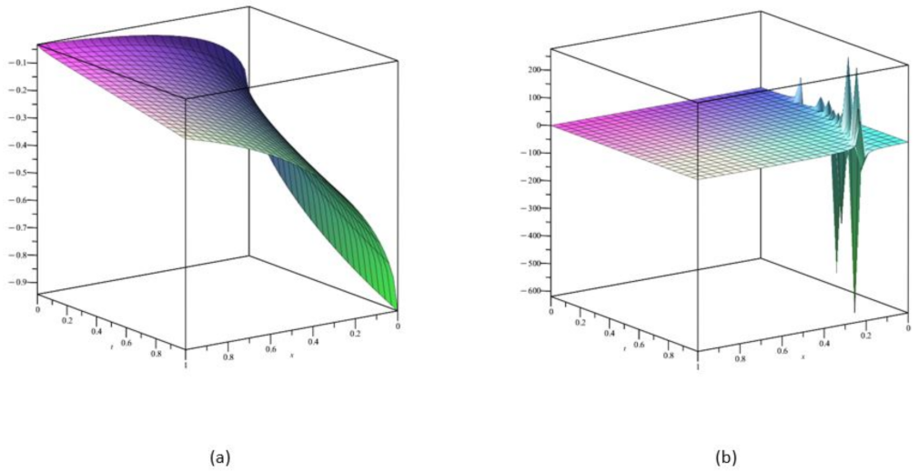
3.1. The Space–Time Fractional Burger-Like Equation

We investigated the Burger-like equation in [29,45], which is a space–time fractional given below.

$${\mathcal{T}}_{M,t}^{\omega ,\delta }u+{\mathcal{T}}_{M,x}^{\omega ,\delta }u+u{\mathcal{T}}_{M,x}^{\omega ,\delta }u+\frac{1}{2}{\mathcal{T}}_{M,x}^{\omega ,\delta }{\mathcal{T}}_{M,x}^{\omega ,\delta }u=0,$$

(11)

where $\omega \in (0,1],0<\delta$. By applying the transformation Equation (4) to this equation, the following ordinary differential equation is gained:

$$(k+m)\frac{dU\left(ϵ\right)}{d\left(ϵ\right)}+\frac{m}{2}U\left(ϵ\right)\frac{dU\left(ϵ\right)}{d\left(ϵ\right)}+\frac{m^2}{2}\frac{d^{2}U\left(ϵ\right)}{d{\left(ϵ\right)}^2}=0.$$

(12)

By integrating Equation (12) once and taking constants of integration as zero, the following equation is found:

$$(k+m)U\left(ϵ\right)+\frac{m}{2}U{\left(ϵ\right)}^2+\frac{m^2}{2}\frac{dU\left(ϵ\right)}{d\left(ϵ\right)}=0.$$

(13)

By balancing the terms of $U^2$ and $\frac{dU\left(ϵ\right)}{d\epsilon }$ in Equation (13), we find $N=1$. For $N=1$, the solution arises through us of (6) as follows:

$$U\left(ϵ\right)=a_{-1}{\left(\frac{G^{\prime }}{G}\right)}^{-1}+a_0+a_1\left(\frac{G^{\prime }}{G}\right),$$

(14)

where $a_{-1},a_0$ and $a_1$ are unknown constants.

By substituting (14) using (7) into (13) and setting the coefficients of all powers of $\left(\frac{G^{\prime }}{G}\right)$ to be zero, nonlinear algebraic equations can be obtained. The occuring algebraic system is solved with Maple to find the values of unknown constants.

$$\begin{array}{cccc}\hfill & {\left(\frac{G^{\prime }}{G}\right)}^{-2}\hfill & \hfill :& \frac{m}{2}{a}_{-1}^2+\frac{m^2}{2}\mu a_{-1}=0,\hfill \\ \hfill & {\left(\frac{G^{\prime }}{G}\right)}^{-1}\hfill & \hfill :& (k+m)a_{-1}+m{a}_{-1}{a}_0+\frac{m^2}{2}\lambda a_{-1}=0,\hfill \\ \hfill & {\left(\frac{G^{\prime }}{G}\right)}^0\hfill & \hfill :& (k+m)a_0+\frac{m}{2}{a}_0^2+m{a}_{-1}{a}_1+\frac{m^2}{2}{a}_{-1}-\frac{m^2}{2}\mu a_1=0,\hfill \\ \hfill & {\left(\frac{G^{\prime }}{G}\right)}^1\hfill & \hfill :& (k+m)a_1+m{a}_0{a}_1-\frac{m^2}{2}\lambda a_1=0,\hfill \\ \hfill & {\left(\frac{G^{\prime }}{G}\right)}^2\hfill & \hfill :& \frac{m}{2}{a}_1^2-\frac{m^2}{2}{a}_1=0.\hfill \end{array}$$

Solving this system of equations through Maple, we obtain the following results:

Result 1: $k=\frac{-m^2\lambda }{2}-m^2\left(\frac{-\lambda \mp \sqrt{{\lambda }^2-4\mu }}{2}\right)-m,a_0=\left(\frac{-\lambda \mp \sqrt{{\lambda }^2-4\mu }}{2}\right)m,a_1=0,a_{-1}=-m\mu$,

Result 2: $k=\frac{m^2\lambda }{2}-m^2\left(\frac{\lambda \mp \sqrt{{\lambda }^2-4\mu }}{2}\right)-m,a_0=\left(\frac{\lambda \mp \sqrt{{\lambda }^2-4\mu }}{2}\right)m,a_1=m,a_{-1}=0$.

The exact solutions to the space–time fractional Burger-Like equation can be obiatained by substituting these results into (14) and taking into account (8)–(10) as follows:

Solution 1:

If ${\lambda }^2-4\mu >0$, the hyperbolic solution is achieved

$$\begin{array}{cc}\hfill & u_1(x,t)=U_{11}\left(ϵ\right)=\left(\frac{-\lambda \mp \sqrt{{\lambda }^2-4\mu }}{2}\right)m\hfill \\ \hfill & -m\mu {\left(-\frac{\lambda }{2}+\frac{\sqrt{{\lambda }^2-4\mu }}{2}\left(\frac{A_{1}sinh\left(\frac{\sqrt{{\lambda }^2-4\mu }}{2}ϵ\right)+A_{2}cosh\left(\frac{\sqrt{{\lambda }^2-4\mu }}{2}ϵ\right)}{A_{1}cosh\left(\frac{\sqrt{{\lambda }^2-4\mu }}{2}ϵ\right)+A_{2}sinh\left(\frac{\sqrt{{\lambda }^2-4\mu }}{2}ϵ\right)}\right)\right)}^{-1}.\hfill \end{array}$$

(15)

If ${\lambda }^2-4\mu =0$, then, the rational solution is found

$$\begin{array}{cc}\hfill & u_2(x,t)=U_{13}\left(ϵ\right)=-\frac{\lambda }{2}m-m\mu \left(-\frac{\lambda }{2}+\frac{A_2}{A_1+A_2ϵ}\right).\hfill \end{array}$$

(16)

In (15) and (16), $ϵ=\frac{\mathsf{\Gamma }(\delta +1)}{\omega }\left[m{x}^{\omega }+\left(\frac{-m^2\lambda }{2}-m^2\left(\frac{-\lambda \mp \sqrt{{\lambda }^2-4\mu }}{2}\right)-m\right)t^{\omega }\right]$.

Solution 2:

If ${\lambda }^2-4\mu >0$, the hyperbolic solution is obtained

$$\begin{array}{cc}\hfill & u_3(x,t)=U_{21}\left(ϵ\right)=\left(\frac{\lambda \mp \sqrt{{\lambda }^2-4\mu }}{2}\right)m\hfill \\ \hfill & +m\left(-\frac{\lambda }{2}+\frac{\sqrt{{\lambda }^2-4\mu }}{2}\left(\frac{A_{1}sinh\left(\frac{\sqrt{{\lambda }^2-4\mu }}{2}ϵ\right)+A_{2}cosh\left(\frac{\sqrt{{\lambda }^2-4\mu }}{2}ϵ\right)}{A_{1}cosh\left(\frac{\sqrt{{\lambda }^2-4\mu }}{2}ϵ\right)+A_{2}sinh\left(\frac{\sqrt{{\lambda }^2-4\mu }}{2}ϵ\right)}\right)\right).\hfill \end{array}$$

(17)

If ${\lambda }^2-4\mu =0$, then, the rational solution is found

$$\begin{array}{cc}\hfill & u_4(x,t)=U_{23}\left(ϵ\right)=m\left(\frac{A_2}{A_1+A_2ϵ}\right).\hfill \end{array}$$

(18)

In (17) and (18), $ϵ=\frac{\mathsf{\Gamma }(\delta +1)}{\omega }\left[m{x}^{\omega }+\left(\frac{m^2\lambda }{2}-m^2\left(\frac{\lambda \mp \sqrt{{\lambda }^2-4\mu }}{2}\right)-m\right)t^{\omega }\right]$.

Figure 1 illustrates the exact solutions of $u(x,t)$ with some particular parameters.

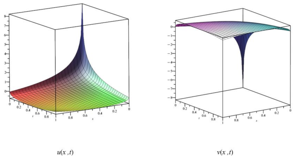
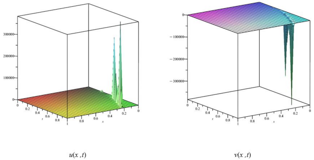
3.2. The Space–Time Fractional Coupled Boussinesq Equation

We examine the space–time fractional coupled Boussinesq equation in [31], which is shown below.

$$\begin{array}{c}{\mathcal{T}}_{M,t}^{\omega ,\delta }u+{\mathcal{T}}_{M,x}^{\omega ,\delta }v=0,\hfill \\ \hfill & {\mathcal{T}}_{M,t}^{\omega ,\delta }v+\gamma {\mathcal{T}}_{M,x}^{\omega ,\delta }\left(u^2\right)-\beta {\mathcal{T}}_{M,x}^{\omega ,\delta }{\mathcal{T}}_{M,x}^{\omega ,\delta }{\mathcal{T}}_{M,x}^{\omega ,\delta }u=0,\hfill \end{array}$$

(19)

where $\omega \in (0,1],0<\delta$. The following ordinary differential equation system is obtained by applying the transformation Equation (4) to above equation for both $u(x,t)$ and $v(x,t)$:

$$\begin{array}{c}k\frac{dU\left(ϵ\right)}{d\left(ϵ\right)}+m\frac{dV\left(ϵ\right)}{d\left(ϵ\right)}=0,\hfill \\ k\frac{dV\left(ϵ\right)}{d\left(ϵ\right)}+\gamma m\frac{d}{d\left(ϵ\right)}\left(U^2\right)-\beta m^3\frac{d^{3}U\left(ϵ\right)}{d{\left(ϵ\right)}^3}=0.\hfill \end{array}$$

(20)

The following system is produced by once-integrating Equation (20) and setting the integration constants to zero:

$$\begin{array}{c}kU+mV=0,\hfill \\ kV+\gamma m{U}^2-\beta m^3\frac{d^{2}U\left(ϵ\right)}{d{\left(ϵ\right)}^2}=0.\hfill \end{array}$$

(21)

From the first equation of Equation (20), we can obtain the following:

$$V=-\frac{k}{m}U.$$

(22)

Substituting Equation (22) into the second equation of Equation (21), we obtain the following differential equation to find the solution of the system:

$$-\frac{k^2}{m}U\left(ϵ\right)+\gamma mU{\left(ϵ\right)}^2-\beta m^3\frac{d^{2}U\left(ϵ\right)}{d{\left(ϵ\right)}^2}=0.$$

(23)

Balancing the terms of $U^2$ and $\frac{d^{2}U\left(ϵ\right)}{d{\epsilon }^2}$ in Equation (21), we obtain $N=2$. For $N=2$, the solution arise with use of (6) as follows:

$$U\left(ϵ\right)=a_{-2}{\left(\frac{G^{\prime }}{G}\right)}^{-2}+a_{-1}{\left(\frac{G^{\prime }}{G}\right)}^{-1}+a_0+a_1\left(\frac{G^{\prime }}{G}\right)+a_2{\left(\frac{G^{\prime }}{G}\right)}^2,$$

(24)

where $a_{-2},a_{-1},a_0,a_1$ and $a_2$ are unknown constants.

Substituting (24) using (7) into (23), we produce nonlinear algebraic equations by setting the coefficients of all powers of $\left(\frac{G^{\prime }}{G}\right)$ to zero. The Maple program is used to solve the arising algebraic system and determine the values of the unidentified constants.

$$\begin{array}{cccc}\hfill & {\left(\frac{G^{\prime }}{G}\right)}^{-4}\hfill & \hfill :& \gamma m^2{a}_{-2}^2-6\beta {\mu }^2{m}^4{a}_{-2}=0,\hfill \\ \hfill & {\left(\frac{G^{\prime }}{G}\right)}^{-3}\hfill & \hfill :& 2\gamma m^2{a}_{-2}{a}_{-1}-10\beta \lambda \mu m^4{a}_{-2}-2\beta {\mu }^2{m}^4{a}_{-1}=0,\hfill \\ \hfill & {\left(\frac{G^{\prime }}{G}\right)}^{-2}\hfill & \hfill :& -k^{2}m{a}_{-2}+\gamma m^2{a}_{-1}^2+2\gamma m^2{a}_{-2}{a}_0-\beta (4{\lambda }^2+8\mu )m^4{a}_{-2}-3\beta \lambda \mu m^4{a}_{-1}=0,\hfill \\ \hfill & {\left(\frac{G^{\prime }}{G}\right)}^{-1}\hfill & \hfill :& -k^{2}m{a}_{-1}+2\gamma m^2{a}_{-2}{a}_{-1}+2\gamma m^2{a}_{-1}{a}_0-6\beta \lambda m^4{a}_{-2}-\beta ({\lambda }^2+2\mu )m^4{a}_{-1}=0,\hfill \\ \hfill & {\left(\frac{G^{\prime }}{G}\right)}^0\hfill & \hfill :& -k^{2}m{a}_0+\gamma m^2{a}_0^2+2\gamma m^2{a}_{-2}{a}_2+2\gamma m^2{a}_{-1}{a}_1-2\beta m^4{a}_{-2}-\beta \lambda m^4{a}_{-1}\hfill \\ \hfill & \hfill & & -\beta \lambda \mu m^4{a}_1-2\beta {\mu }^2{m}^4{a}_2=0,\hfill \\ \hfill & {\left(\frac{G^{\prime }}{G}\right)}^1\hfill & \hfill :& -k^{2}m{a}_1+2\gamma m^2{a}_0{a}_1+2\gamma m^2{a}_{-1}{a}_2-6\beta \lambda \mu m^4{a}_2-\beta ({\lambda }^2+2\mu )m^4{a}_1=0,\hfill \\ \hfill & {\left(\frac{G^{\prime }}{G}\right)}^2\hfill & \hfill :& -k^{2}m{a}_2+\gamma m^2{a}_1^2+2\gamma m^2{a}_0{a}_2-\beta (4{\lambda }^2+8\mu )m^4{a}_2-3\beta \lambda m^4{a}_1=0,\hfill \\ \hfill & {\left(\frac{G^{\prime }}{G}\right)}^3\hfill & \hfill :& 2\gamma m^2{a}_1{a}_2-10\beta \lambda m^4{a}_2-2\beta m^4{a}_1=0,\hfill \\ \hfill & {\left(\frac{G^{\prime }}{G}\right)}^4\hfill & \hfill :& \gamma m^2{a}_2^2-6\beta m^4{a}_2=0.\hfill \end{array}$$

The results of solving this system of equations using Maple are as follows:

Result 1: $k=\mp m\sqrt{\beta m(-{\lambda }^2+4\mu )},a_0=\frac{6\beta \mu m^2}{\gamma },a_1=\frac{6\beta \lambda m^2}{\gamma },a_2=\frac{6\beta m^2}{\gamma },a_{-1}=a_{-2}=0$,

Result 2: $k=\mp m\sqrt{\beta m({\lambda }^2-4\mu )},a_0=\frac{\beta ({\lambda }^2+2\mu )m^2}{\gamma },a_1=\frac{6\beta \lambda m^2}{\gamma },a_2=\frac{6\beta m^2}{\gamma },a_{-1}=a_{-2}=0$,

Result 3: $k=\mp m\sqrt{\beta m(-{\lambda }^2+4\mu )},a_{-2}=\frac{6\beta {\mu }^2{m}^2}{\gamma },a_{-1}=\frac{6\beta \lambda \mu m^2}{\gamma },a_0=\frac{6\beta \mu m^2}{\gamma },a_1=a_2=0$,

Result 4: $k=\mp m\sqrt{\beta m({\lambda }^2-4\mu )},a_{-2}=\frac{6\beta {\mu }^2{m}^2}{\gamma },a_{-1}=\frac{6\beta \lambda \mu m^2}{\gamma },a_0=\frac{\beta ({\lambda }^2+2\mu )m^2}{\gamma },a_1=a_2=0$

By entering these results into (24) and taking into consideration (8)–(10), we can obtain the space–time fractional coupled Boussinesq equation’s exact solutions as follows:

Solution 1:

If ${\lambda }^2-4\mu <0$, the trigonometric solution is acquired

$$\begin{array}{cc}\hfill & u_1(x,t)=U_{12}\left(ϵ\right)=\frac{6\beta \mu m^2}{\gamma }\hfill \\ \hfill & +\frac{6\beta \lambda m^2}{\gamma }\left(-\frac{\lambda }{2}+\frac{\sqrt{4\mu -{\lambda }^2}}{2}\left(\frac{-A_{1}sin\left(\frac{\sqrt{4\mu -{\lambda }^2}}{2}ϵ\right)+A_{2}cos\left(\frac{\sqrt{4\mu -{\lambda }^2}}{2}ϵ\right)}{A_{1}cos\left(\frac{\sqrt{4\mu -{\lambda }^2}}{2}ϵ\right)+A_{2}sin\left(\frac{\sqrt{4\mu -{\lambda }^2}}{2}ϵ\right)}\right)\right)\hfill \\ \hfill & +\frac{6\beta m^2}{\gamma }{\left(-\frac{\lambda }{2}+\frac{\sqrt{4\mu -{\lambda }^2}}{2}\left(\frac{-A_{1}sin\left(\frac{\sqrt{4\mu -{\lambda }^2}}{2}ϵ\right)+A_{2}cos\left(\frac{\sqrt{4\mu -{\lambda }^2}}{2}ϵ\right)}{A_{1}cos\left(\frac{\sqrt{4\mu -{\lambda }^2}}{2}ϵ\right)+A_{2}sin\left(\frac{\sqrt{4\mu -{\lambda }^2}}{2}ϵ\right)}\right)\right)}^2.\hfill \end{array}$$

(25)

From Equation (22),

$$\begin{array}{cc}\hfill & v_1(x,t)=-\frac{k}{m}[\frac{6\beta \mu m^2}{\gamma }\hfill \\ \hfill & +\frac{6\beta \lambda m^2}{\gamma }\left(-\frac{\lambda }{2}+\frac{\sqrt{4\mu -{\lambda }^2}}{2}\left(\frac{-A_{1}sin\left(\frac{\sqrt{4\mu -{\lambda }^2}}{2}ϵ\right)+A_{2}cos\left(\frac{\sqrt{4\mu -{\lambda }^2}}{2}ϵ\right)}{A_{1}cos\left(\frac{\sqrt{4\mu -{\lambda }^2}}{2}ϵ\right)+A_{2}sin\left(\frac{\sqrt{4\mu -{\lambda }^2}}{2}ϵ\right)}\right)\right)\hfill \\ \hfill & +\frac{6\beta m^2}{\gamma }{\left(-\frac{\lambda }{2}+\frac{\sqrt{4\mu -{\lambda }^2}}{2}\left(\frac{-A_{1}sin\left(\frac{\sqrt{4\mu -{\lambda }^2}}{2}ϵ\right)+A_{2}cos\left(\frac{\sqrt{4\mu -{\lambda }^2}}{2}ϵ\right)}{A_{1}cos\left(\frac{\sqrt{4\mu -{\lambda }^2}}{2}ϵ\right)+A_{2}sin\left(\frac{\sqrt{4\mu -{\lambda }^2}}{2}ϵ\right)}\right)\right)}^2].\hfill \end{array}$$

(26)

If ${\lambda }^2-4\mu =0$, then the rational solution is found

$$\begin{array}{cc}\hfill & u_2(x,t)=U_{13}\left(ϵ\right)=\frac{6\beta \mu m^2}{\gamma }+\frac{6\beta \lambda m^2}{\gamma }\left(-\frac{\lambda }{2}+\frac{A_2}{A_1+A_2ϵ}\right)\hfill \\ \hfill & +\frac{6\beta m^2}{\gamma }{\left(-\frac{\lambda }{2}+\frac{A_2}{A_1+A_2ϵ}\right)}^2.\hfill \end{array}$$

(27)

From Equation (22),

$$\begin{array}{cc}\hfill & v_2(x,t)=-\frac{k}{m}[\frac{6\beta \mu m^2}{\gamma }+\frac{6\beta \lambda m^2}{\gamma }\left(-\frac{\lambda }{2}+\frac{A_2}{A_1+A_2ϵ}\right)\hfill \\ \hfill & +\frac{6\beta m^2}{\gamma }{\left(-\frac{\lambda }{2}+\frac{A_2}{A_1+A_2ϵ}\right)}^2].\hfill \end{array}$$

(28)

In (25)–(28), $ϵ=\frac{\mathsf{\Gamma }(\delta +1)}{\omega }\left[m{x}^{\omega }+\left(\mp m\sqrt{\beta m(-{\lambda }^2+4\mu )}\right)t^{\omega }\right]$.

Figure 2 and Figure 3 show the exact solutions of $u(x,t)$ and $v(x,t)$ with some particular parameters.

Solution 2:

If ${\lambda }^2-4\mu >0$, the hyperbolic solution is found

$$\begin{array}{cc}\hfill & u_3(x,t)=U_{21}\left(ϵ\right)=\frac{\beta ({\lambda }^2+2\mu )m^2}{\gamma }\hfill \\ \hfill & +\frac{6\beta \lambda m^2}{\gamma }\left(-\frac{\lambda }{2}+\frac{\sqrt{{\lambda }^2-4\mu }}{2}\left(\frac{A_{1}sinh\left(\frac{\sqrt{{\lambda }^2-4\mu }}{2}ϵ\right)+A_{2}cosh\left(\frac{\sqrt{{\lambda }^2-4\mu }}{2}ϵ\right)}{A_{1}cosh\left(\frac{\sqrt{{\lambda }^2-4\mu }}{2}ϵ\right)+A_{2}sinh\left(\frac{\sqrt{{\lambda }^2-4\mu }}{2}ϵ\right)}\right)\right)\hfill \\ \hfill & +\frac{6\beta m^2}{\gamma }{\left(-\frac{\lambda }{2}+\frac{\sqrt{{\lambda }^2-4\mu }}{2}\left(\frac{A_{1}sinh\left(\frac{\sqrt{{\lambda }^2-4\mu }}{2}ϵ\right)+A_{2}cosh\left(\frac{\sqrt{{\lambda }^2-4\mu }}{2}ϵ\right)}{A_{1}cosh\left(\frac{\sqrt{{\lambda }^2-4\mu }}{2}ϵ\right)+A_{2}sinh\left(\frac{\sqrt{{\lambda }^2-4\mu }}{2}ϵ\right)}\right)\right)}^2.\hfill \end{array}$$

(29)

From Equation (22),

$$\begin{array}{cc}\hfill & v_3(x,t)=-\frac{k}{m}[\frac{\beta ({\lambda }^2+2\mu )m^2}{\gamma }\hfill \\ \hfill & +\frac{6\beta \lambda m^2}{\gamma }\left(-\frac{\lambda }{2}+\frac{\sqrt{{\lambda }^2-4\mu }}{2}\left(\frac{A_{1}sinh\left(\frac{\sqrt{{\lambda }^2-4\mu }}{2}ϵ\right)+A_{2}cosh\left(\frac{\sqrt{{\lambda }^2-4\mu }}{2}ϵ\right)}{A_{1}cosh\left(\frac{\sqrt{{\lambda }^2-4\mu }}{2}ϵ\right)+A_{2}sinh\left(\frac{\sqrt{{\lambda }^2-4\mu }}{2}ϵ\right)}\right)\right)\hfill \\ \hfill & +\frac{6\beta m^2}{\gamma }{\left(-\frac{\lambda }{2}+\frac{\sqrt{{\lambda }^2-4\mu }}{2}\left(\frac{A_{1}sinh\left(\frac{\sqrt{{\lambda }^2-4\mu }}{2}ϵ\right)+A_{2}cosh\left(\frac{\sqrt{{\lambda }^2-4\mu }}{2}ϵ\right)}{A_{1}cosh\left(\frac{\sqrt{{\lambda }^2-4\mu }}{2}ϵ\right)+A_{2}sinh\left(\frac{\sqrt{{\lambda }^2-4\mu }}{2}ϵ\right)}\right)\right)}^2].\hfill \end{array}$$

(30)

If ${\lambda }^2-4\mu =0$, then the rational solution is found

$$\begin{array}{cc}\hfill & u_4(x,t)=U_{23}\left(ϵ\right)=\frac{\beta ({\lambda }^2+2\mu )m^2}{\gamma }+\frac{6\beta \lambda m^2}{\gamma }\left(-\frac{\lambda }{2}+\frac{A_2}{A_1+A_2ϵ}\right)\hfill \\ \hfill & +\frac{6\beta m^2}{\gamma }{\left(-\frac{\lambda }{2}+\frac{A_2}{A_1+A_2ϵ}\right)}^2.\hfill \end{array}$$

(31)

From Equation (22),

$$\begin{array}{cc}\hfill & v_4(x,t)=-\frac{k}{m}[\frac{\beta ({\lambda }^2+2\mu )m^2}{\gamma }+\frac{6\beta \lambda m^2}{\gamma }\left(-\frac{\lambda }{2}+\frac{A_2}{A_1+A_2ϵ}\right)\hfill \\ \hfill & +\frac{6\beta m^2}{\gamma }{\left(-\frac{\lambda }{2}+\frac{A_2}{A_1+A_2ϵ}\right)}^2].\hfill \end{array}$$

(32)

In (29)–(32), $ϵ=\frac{\mathsf{\Gamma }(\delta +1)}{\omega }\left[m{x}^{\omega }+\left(\mp m\sqrt{\beta m({\lambda }^2-4\mu )}\right)t^{\omega }\right]$.

Solution 3:

If ${\lambda }^2-4\mu <0$, the trigonometric solution is acquired

$$\begin{array}{cc}\hfill & u_5(x,t)=U_{32}\left(ϵ\right)=\frac{6\beta \mu m^2}{\gamma }\hfill \\ \hfill & +\frac{6\beta \lambda \mu m^2}{\gamma }{\left(-\frac{\lambda }{2}+\frac{\sqrt{4\mu -{\lambda }^2}}{2}\left(\frac{-A_{1}sin\left(\frac{\sqrt{4\mu -{\lambda }^2}}{2}ϵ\right)+A_{2}cos\left(\frac{\sqrt{4\mu -{\lambda }^2}}{2}ϵ\right)}{A_{1}cos\left(\frac{\sqrt{4\mu -{\lambda }^2}}{2}ϵ\right)+A_{2}sin\left(\frac{\sqrt{4\mu -{\lambda }^2}}{2}ϵ\right)}\right)\right)}^{-1}\hfill \\ \hfill & +\frac{6\beta {\mu }^2{m}^2}{\gamma }{\left(-\frac{\lambda }{2}+\frac{\sqrt{4\mu -{\lambda }^2}}{2}\left(\frac{-A_{1}sin\left(\frac{\sqrt{4\mu -{\lambda }^2}}{2}ϵ\right)+A_{2}cos\left(\frac{\sqrt{4\mu -{\lambda }^2}}{2}ϵ\right)}{A_{1}cos\left(\frac{\sqrt{4\mu -{\lambda }^2}}{2}ϵ\right)+A_{2}sin\left(\frac{\sqrt{4\mu -{\lambda }^2}}{2}ϵ\right)}\right)\right)}^{-2}.\hfill \end{array}$$

(33)

From Equation (22),

$$\begin{array}{cc}\hfill & v_5(x,t)=-\frac{k}{m}[\frac{6\beta \mu m^2}{\gamma }\hfill \\ \hfill & +\frac{6\beta \lambda \mu m^2}{\gamma }{\left(-\frac{\lambda }{2}+\frac{\sqrt{4\mu -{\lambda }^2}}{2}\left(\frac{-A_{1}sin\left(\frac{\sqrt{4\mu -{\lambda }^2}}{2}ϵ\right)+A_{2}cos\left(\frac{\sqrt{4\mu -{\lambda }^2}}{2}ϵ\right)}{A_{1}cos\left(\frac{\sqrt{4\mu -{\lambda }^2}}{2}ϵ\right)+A_{2}sin\left(\frac{\sqrt{4\mu -{\lambda }^2}}{2}ϵ\right)}\right)\right)}^{-1}\hfill \\ \hfill & +\frac{6\beta {\mu }^2{m}^2}{\gamma }{\left(-\frac{\lambda }{2}+\frac{\sqrt{4\mu -{\lambda }^2}}{2}\left(\frac{-A_{1}sin\left(\frac{\sqrt{4\mu -{\lambda }^2}}{2}ϵ\right)+A_{2}cos\left(\frac{\sqrt{4\mu -{\lambda }^2}}{2}ϵ\right)}{A_{1}cos\left(\frac{\sqrt{4\mu -{\lambda }^2}}{2}ϵ\right)+A_{2}sin\left(\frac{\sqrt{4\mu -{\lambda }^2}}{2}ϵ\right)}\right)\right)}^{-2}].\hfill \end{array}$$

(34)

If ${\lambda }^2-4\mu =0$, then the rational solution is found

$$\begin{array}{cc}\hfill & u_6(x,t)=U_{33}\left(ϵ\right)=\frac{6\beta \mu m^2}{\gamma }+\frac{6\beta \lambda \mu m^2}{\gamma }{\left(-\frac{\lambda }{2}+\frac{A_2}{A_1+A_2ϵ}\right)}^{-1}\hfill \\ \hfill & +\frac{6\beta {\mu }^2{m}^2}{\gamma }{\left(-\frac{\lambda }{2}+\frac{A_2}{A_1+A_2ϵ}\right)}^{-2}.\hfill \end{array}$$

(35)

From Equation (22),

$$\begin{array}{cc}\hfill & v_6(x,t)=-\frac{k}{m}[\frac{6\beta \mu m^2}{\gamma }+\frac{6\beta \lambda \mu m^2}{\gamma }{\left(-\frac{\lambda }{2}+\frac{A_2}{A_1+A_2ϵ}\right)}^{-1}\hfill \\ \hfill & +\frac{6\beta {\mu }^2{m}^2}{\gamma }{\left(-\frac{\lambda }{2}+\frac{A_2}{A_1+A_2ϵ}\right)}^{-2}].\hfill \end{array}$$

(36)

In (33)–(36), $ϵ=\frac{\mathsf{\Gamma }(\delta +1)}{\omega }\left[m{x}^{\omega }+\left(\mp m\sqrt{\beta m(-{\lambda }^2+4\mu )}\right)t^{\omega }\right]$.

Solution 4:

If ${\lambda }^2-4\mu >0$, the hyperbolic solution is achieved

$$\begin{array}{cc}\hfill & u_7(x,t)=U_{41}\left(ϵ\right)=\frac{\beta ({\lambda }^2+2\mu )m^2}{\gamma }\hfill \\ \hfill & +\frac{6\beta \lambda \mu m^2}{\gamma }{\left(-\frac{\lambda }{2}+\frac{\sqrt{{\lambda }^2-4\mu }}{2}\left(\frac{A_{1}sinh\left(\frac{\sqrt{{\lambda }^2-4\mu }}{2}ϵ\right)+A_{2}cosh\left(\frac{\sqrt{{\lambda }^2-4\mu }}{2}ϵ\right)}{A_{1}cosh\left(\frac{\sqrt{{\lambda }^2-4\mu }}{2}ϵ\right)+A_{2}sinh\left(\frac{\sqrt{{\lambda }^2-4\mu }}{2}ϵ\right)}\right)\right)}^{-1}\hfill \\ \hfill & +\frac{6\beta {\mu }^2{m}^2}{\gamma }{\left(-\frac{\lambda }{2}+\frac{\sqrt{{\lambda }^2-4\mu }}{2}\left(\frac{A_{1}sinh\left(\frac{\sqrt{{\lambda }^2-4\mu }}{2}ϵ\right)+A_{2}cosh\left(\frac{\sqrt{{\lambda }^2-4\mu }}{2}ϵ\right)}{A_{1}cosh\left(\frac{\sqrt{{\lambda }^2-4\mu }}{2}ϵ\right)+A_{2}sinh\left(\frac{\sqrt{{\lambda }^2-4\mu }}{2}ϵ\right)}\right)\right)}^{-2}.\hfill \end{array}$$

(37)

From Equation (22),

$$\begin{array}{cc}\hfill & v_7(x,t)=-\frac{k}{m}[\frac{\beta ({\lambda }^2+2\mu )m^2}{\gamma }\hfill \\ \hfill & +\frac{6\beta \lambda \mu m^2}{\gamma }{\left(-\frac{\lambda }{2}+\frac{\sqrt{{\lambda }^2-4\mu }}{2}\left(\frac{A_{1}sinh\left(\frac{\sqrt{{\lambda }^2-4\mu }}{2}ϵ\right)+A_{2}cosh\left(\frac{\sqrt{{\lambda }^2-4\mu }}{2}ϵ\right)}{A_{1}cosh\left(\frac{\sqrt{{\lambda }^2-4\mu }}{2}ϵ\right)+A_{2}sinh\left(\frac{\sqrt{{\lambda }^2-4\mu }}{2}ϵ\right)}\right)\right)}^{-1}\hfill \\ \hfill & +\frac{6\beta {\mu }^2{m}^2}{\gamma }{\left(-\frac{\lambda }{2}+\frac{\sqrt{{\lambda }^2-4\mu }}{2}\left(\frac{A_{1}sinh\left(\frac{\sqrt{{\lambda }^2-4\mu }}{2}ϵ\right)+A_{2}cosh\left(\frac{\sqrt{{\lambda }^2-4\mu }}{2}ϵ\right)}{A_{1}cosh\left(\frac{\sqrt{{\lambda }^2-4\mu }}{2}ϵ\right)+A_{2}sinh\left(\frac{\sqrt{{\lambda }^2-4\mu }}{2}ϵ\right)}\right)\right)}^{-2}].\hfill \end{array}$$

(38)

If ${\lambda }^2-4\mu =0$, then the rational solution is found

$$\begin{array}{cc}\hfill & u_8(x,t)=U_{43}\left(ϵ\right)=\frac{\beta ({\lambda }^2+2\mu )m^2}{\gamma }+\frac{6\beta \lambda \mu m^2}{\gamma }{\left(-\frac{\lambda }{2}+\frac{A_2}{A_1+A_2ϵ}\right)}^{-1}\hfill \\ \hfill & +\frac{6\beta {\mu }^2{m}^2}{\gamma }{\left(-\frac{\lambda }{2}+\frac{A_2}{A_1+A_2ϵ}\right)}^{-2}.\hfill \end{array}$$

(39)

From Equation (22),

$$\begin{array}{cc}\hfill & v_8(x,t)=-\frac{k}{m}[\frac{\beta ({\lambda }^2+2\mu )m^2}{\gamma }+\frac{6\beta \lambda \mu m^2}{\gamma }{\left(-\frac{\lambda }{2}+\frac{A_2}{A_1+A_2ϵ}\right)}^{-1}\hfill \\ \hfill & +\frac{6\beta {\mu }^2{m}^2}{\gamma }{\left(-\frac{\lambda }{2}+\frac{A_2}{A_1+A_2ϵ}\right)}^{-2}].\hfill \end{array}$$

(40)

In (37)–(40), $ϵ=\frac{\mathsf{\Gamma }(\delta +1)}{\omega }\left[m{x}^{\omega }+\left(\mp m\sqrt{\beta m({\lambda }^2-4\mu )}\right)t^{\omega }\right]$.

4. Results and Discussions

In this section, from a physical point of view, we discuss the obtained solutions to the space–time fractional Burger-like equation and the space–time coupled Boussinesq equation with the M-truncated time derivative, which are gained using the above-mentioned method. In order to verify the physical meaning of the mathematical models, we implemented several 3D plots and illustrations of the obtained solutions. Moreover, the effect of the fractional derivatives and the method on the solution of equations are mentioned.

Firstly, we plotted Equation (17), and as shown in Figure 1, we demonstrate the appropriate hyperbolic behavior of the obtained analytical solutions. In Figure 1a, the hyperbolic solution of (17) is plotted when $\lambda =2,\mu =0.5,A_1=2,A_2=m=1,\omega =0.5$. In Figure 1b, the real solutions of (17) are plotted when $\lambda =2,\mu =A_1=A_2=m=1,\omega =0.5$.

The plots for Equations (25) and (26) are presented in Figure 2. The trigonometric solution of (25) and (26) are plotted with $\lambda =1,\gamma =6,A_1=A_2=m=\beta =1,\mu =\omega =0.5$.

Finally, the plots for Equations (27) and (28) are presented in Figure 3. The real solution of (27) and (28) are plotted with $\lambda =1,\gamma =6,A_1=A_2=m=\beta =1,\mu =\omega =0.5$.

It has been proven that the extended ${\mathrm{G}}^{\prime }/\mathrm{G}$-method is very useful and efficient and can be used in a wide variety of solutions. Hyperbolic, trigonometric, and rational solutions have clearly emerged with the distinctiveness and restrictive feature of the method. As a result, much newer and clearer solutions have been obtained. Fractional calculus is a new research field that has attracted many researchers, and although many studies have attempted to explain the physical meaning of fractional derivatives, it is still an open problem.

5. Conclusions

In this work, two nonlinear partial fractional differential equations were solved with M-truncated derivative using the extended ${\mathrm{G}}^{\prime }/\mathrm{G}$-method. Many novel exact solutions to the space–time fractional coupled Boussinesq equation and the space–time fractional coupled Burger-like equation were successfully found as applications. The extended ${\mathrm{G}}^{\prime }/\mathrm{G}$-method analysis of the aforementioned models was revealed using a thorough list of various solutions, including trigonometric, hyperbolic, and rational ones. It is important to note that the found solutions are novel since a new fractional derivative was used to explore the model’s new form. The fact that the solutions to the Equations (11) and (19) were obtained utilizing various derivatives and methods makes it clear that our results are original and have not previously been explored in the literature. The fact that the solutions to the equations in [29,31,45] were obtained using various derivatives methods demonstrates additionally attests to the novelty of our results.

The results of this study add to the corpus of literature by offering insightful explanations of several nonlinear systems. The solution described here, to our knowledge, have not been previously attempted. The outcomes also showed that Maple, a symbolic program computing system, simplifies, strengthens, and accelerates the suggested method as a helpful mathematical tool. It is worth considering that the recommended method may be used to solve a variety of nonlinear evolution issues in mathematical physics. The findings of the study may have an impact on how various physical issues are understood.

References

1. Yildirim, O.; Uzun, M. Weak solvability of the unconditionally stable difference scheme for the coupled sine-Gordon system. Nonlinear Anal. Model. Control. 2020, 25, 997–1014. [Google Scholar] [CrossRef]
2. Yildirim, O.; Uzun, M. Numer. Solut. High Order Stable Differ. Schemes Hyperbolic Multipoint Nonlocal Bound. Value Probl. Appl. Math. Comput. 2015, 25, 210–218. [Google Scholar]
3. Yildirim, O.; Caglak, S. Lie point symmetries of difference equation for nonlinear sine-Gordon equation. Phys. Scr. 2019, 94, 085219. [Google Scholar] [CrossRef]
4. Ozkan, A. Analytical Solutions of the Nonlinear (2 + 1)-Dimensional Soliton Equation by Using Some Methods. J. Eng. Technol. Appl. Sci. 2022, 7, 141–155. [Google Scholar]
5. Fang, Y.; Wu, G.Z.; Wang, Y.Y.; Dai, C.Q. Data-driven femtosecond optical soliton excitations and parameters discovery of the high-order NLSE using the PINN. Nonlinear Dyn. 2021, 105, 603–616. [Google Scholar] [CrossRef]
6. Fang, Y.; Wu, G.Z.; Wen, X.K.; Wang, Y.Y.; Dai, C.Q. Predicting certain vector optical solitons via the conservation-law deep-learning method. Opt. Laser Technol. 2022, 155, 108428. [Google Scholar] [CrossRef]
7. Bo, W.B.; Wang, R.R.; Fang, Y.; Wang, Y.Y.; Dai, C.Q. Prediction and dynamical evolution of multipole soliton families in fractional Schrödinger equation with the PT-symmetric potential and saturable nonlinearity. Nonlinear Dyn. 2023, 111, 1577–1588. [Google Scholar] [CrossRef]
8. Cheng, X.Y.; Wang, L.Z. Invariant analysis, exact solutions and conservation laws of (2 + 1)-dimensional time fractional Navier-Stokes equations. Proc. R. Soc. A 2022, 477, 20210220. [Google Scholar] [CrossRef]
9. Yang, Y.; Wang, L.Z. Lie symmetry analysis, conservation laws and separation variable type solutions of the time fractional Porous Medium equation. Wave. Random. Complex. 2020, 49, 1–20. [Google Scholar] [CrossRef]
10. Cheng, X.Y.; Hou, J.; Wang, L.Z. Lie symmetry analysis, invariant subspace method and q-homotopy analysis method for solving fractional system of single-walled carbon nanotube. Comput. Appl. Math. 2021, 40, 1–17. [Google Scholar] [CrossRef]
11. Wang, M.M.; Shen, S.F.; Wang, L.Z. Lie symmetry analysis, optimal system and conservation laws of a new (2 + 1)-dimensional KdV system. Commun. Theor. Phys. 2021, 73, 085004. [Google Scholar] [CrossRef]
12. Wang, L.Z.; Wang, D.J.; Shen, S.F.; Huang, Q. Lie point symmetry analysis of the Harry-Dym type equation with Riemann-Liouville fractional derivative. Acta. Math. Appl. Sin. 2018, 34, 469–477. [Google Scholar] [CrossRef]
13. Kudryashov, N.A. One method for finding exact solutions of nonlinear differential equations. Commun. Nonlinear Sci. Numer. Simulat. 2012, 17, 2048–2053. [Google Scholar] [CrossRef] [Green Version]
14. Akbulut, A.; Kaplan, M.; Tascan, F. The investigation of exact solutions of nonlinear partial differential equations by using exp(-Φ(ε)) method. Optik 2017, 132, 382–387. [Google Scholar] [CrossRef]
15. Ozkan, E.M.; Ozkan, A. On exact solutions of some important nonlinear conformable time-fractional differential equations. Sema J. 2022, 79, 1–16. [Google Scholar]
16. Ozkan, A. On the soliton solutions of some time conformable equations in fluid dynamics. Int. Mod. Phys. B 2023, 2450027. [Google Scholar] [CrossRef]
17. Ozkan, E.M.; Ozkan, A. The Soliton Solutions for Some Nonlinear Fractional Differential Equations with Beta-Derivative. Axioms 2021, 10, 1–15. [Google Scholar] [CrossRef]
18. Gómez, S.; Cesar, A. A nonlinear fractional Sharma–Tasso–Olver equation. App. Math. Comput. 2015, 266, 385–389. [Google Scholar] [CrossRef]
19. Lu, B. The first integral method for some time fractional differential equations. J. Math. Anal. Appl. 2012, 395, 684–693. [Google Scholar] [CrossRef] [Green Version]
20. Zheng, B. Exp-function method for solving fractional partial differential equations. Sci. World J. 2013, 2013, 465723. [Google Scholar] [CrossRef] [Green Version]
21. Ozkan, E.M. New Exact Solutions of Some Important Nonlinear Fractional Partial Differential Equations with Beta Derivative. Fractal Fract. 2022, 6, 173. [Google Scholar] [CrossRef]
22. Ozkan, E.M.; Akar, M. Analytical solutions of (2 + 1)-dimensional time conformable Schrödinger equation using improved sub-equation method. Optik 2022, 267, 169660. [Google Scholar] [CrossRef]
23. Akar, M.; Ozkan, E.M. On exact solutions of the (2 + 1)-dimensional time conformable Maccari system. Int. Mod. Phys. B 2023, 1–12. [Google Scholar] [CrossRef]
24. Matinfar, M.; Eslami, M.; Kordy, M. The functional variable method for solving thefractional Korteweg de Vries equations and the coupled Korteweg de Vries equations. Pramana J. Phys. 2015, 85, 583–592. [Google Scholar] [CrossRef]
25. Zogheib, B.; Tohidi, E.; Baskonus, H.M.; Cattani, C. Method of lines for multi-dimensional coupled viscous Burgers’ equations via nodal Jacobi spectral collocation method. Phys. Scr. 2021, 96, 124011. [Google Scholar] [CrossRef]
26. Sulaiman, T.A.; Yavuz, M.; Bulut, H.; Baskonus, H.M. Investigation of the fractional coupled viscous Burgers’ equation involving Mittag-Leffler kernel. Phys. Stat. Mech. Appl. 2019, 527, 121126. [Google Scholar] [CrossRef]
27. Bulut, H.; Tuz, M.; Akturk, T. New Multiple Solution to the Boussinesq Equation and the Burgers-Like Equation. J. Appl. Math. 2013, 2013, 952614. [Google Scholar] [CrossRef]
28. Gencoglu, M.T. Complex Solution for Burger-Like Equation. Turk. J. Math. 2013, 8, 121–123. [Google Scholar]
29. Eskandari, E.M.; Taghizadeh, N. Exact Solutions of Two Nonlinear Space–Time Fractional Differential Equations by Application of Exp-function Method. Appl. Appl. Math. Int. J. 2020, 15, 1–8. [Google Scholar]
30. Madsen, P.A.; Murray, R.; Sorensen, O.R. A new form of the Boussinesq equations with improved linear dispersion characteristics. Coast Engl. J. 1991, 15, 371–388. [Google Scholar] [CrossRef]
31. Yaslan, H.C.; Girgin, A. Exp-function method for the conformable Space–Time fractional STO, ZKBBM and coupled Boussinesq equations. Arab. J. Basic Appl. Sci. 2019, 26, 163–170. [Google Scholar] [CrossRef] [Green Version]
32. Sahadevan, R.; Prakash, P. Exact solutions and maximal dimension of invariant subspaces of time fractional coupled nonlinear partial differential equations. Commun. Nonlinear Sci. Numer. Simulat. 2017, 42, 158–177. [Google Scholar] [CrossRef]
33. Hosseini, K.; Bekir, A.; Ansari, R. Exact solutions of nonlinear conformable time-fractional Boussinesq equations using the exp(-ϕ(ε))-expansion method. Opt. Quant. Electron. 2017, 49, 131. [Google Scholar] [CrossRef]
34. Triki, H.; Kara, A.H.; Biswas, A. Domain walls to Boussinesq-type equations in (2 + 1)-dimensions. Indian J. Phys. 2014, 88, 751–755. [Google Scholar] [CrossRef]
35. Abazari, R.; Jamshidzadeh, S.; Biswas, A. Solitary wave solutions of coupled Boussinesq equation. Complexity 2016, 21, 151–155. [Google Scholar] [CrossRef]
36. Abazari, R.; Jamshidzadeh, S.; Biswas, A. Multi soliton solutions based on interactions of basic traveling waves with an application to the nonlocal Boussinesq equation. Acta Phys. Pol. B 2016, 47, 1101–1112. [Google Scholar]
37. Biswas, A.; Kara, A.H.; Moraru, L.; Triki, H.; Moshokoa, S.P. Shallow water waves modeled by the Boussinesq equation having logarithmic non linearity. Proc. Rom. Acad. Ser. A 2017, 18, 144–149. [Google Scholar]
38. Biswas, A.; Ekici, M.; Sonmezoglu, A. Gaussian solitary waves to Boussinesq equation with dual dispersion and logarithmic non linearity. Nonlinear Anal. Model. Control. 2018, 23, 942–950. [Google Scholar] [CrossRef]
39. Jawad, A.J.M.; Petković, M.D.; Laketa, P.; Biswas, A. Dynamics of shallow water waves with Boussinesq equation. Sci. Iran. B 2013, 20, 179–184. [Google Scholar] [CrossRef] [Green Version]
40. Sousa, J.V.D.C.; de Oliveira, E.C. A new truncated M-fractional derivative type unifying some fractional derivative types with classical properties. Int. J. Anal. Appl. 2018, 16, 83–96. [Google Scholar]
41. Salahshour, S.; Ahmadian, A.; Abbasbandy, S.; Baleanu, D. M-fractional derivative under interval uncertainty: Theory, properties and applications. Chaos Solitons Fractals 2018, 117, 84–93. [Google Scholar] [CrossRef]
42. Zayed, E.M.; Amer, A.; Shohib, R.M. Exact traveling wave solutions for nonlinear fractional partial differential equations using the improved (G’/G)-expansion method. Int. J. Eng. Appl. Sci. 2014, 7, 18–31. [Google Scholar]
43. Yusuf, A.; Inc, M.; Baleanu, D. Optical Solitons with M-Truncated and Beta Derivatives in Nonlinear Optics. Front. Phys. 2019, 7, 126. [Google Scholar] [CrossRef] [Green Version]
44. Zafar, A.; Bekir, A.; Raheel, M.; Razzaq, W. Optical soliton solutions to Biswas–Arshed model with truncated M-fractional derivative. Optik 2020, 222, 165355. [Google Scholar] [CrossRef]
45. Yaslan, H.C.; Girgin, A. (G’/G)-expansion Method for the Conformable Space–Time Fractional Jimbo-Miwa and Burger-like Equations. Math. Sci. Appl. Notes 2019, 7, 47–53. [Google Scholar]
Figure 1. Graphical representation of Equation (17).
Fractalfract 07 00255 g001
Figure 2. Graphical illustrations of Equations (25) and (26).
Fractalfract 07 00255 g002
Figure 3. Graphical representations of Equations (27) and (28).
Fractalfract 07 00255 g003
Disclaimer/Publisher’s Note: The statements, opinions and data contained in all publications are solely those of the individual author(s) and contributor(s) and not of MDPI and/or the editor(s). MDPI and/or the editor(s) disclaim responsibility for any injury to people or property resulting from any ideas, methods, instructions or products referred to in the content.