Article

The Influence of the Fractal Dimension on the Mechanical Behaviors of the Soil–Rock Mixture: A Case Study from Southwest China

1
School of Architecture and Civil Engineering, Shenyang University of Technology, Shenyang 110870, China
2
State Key Laboratory of Geomechanics and Geotechnical Engineering, Institute of Rock and Soil Mechanics, Chinese Academy of Sciences, Wuhan 430071, China
3
School of Engineering Science, University of Chinese Academy of Sciences, Beijing 100049, China
4
Key Laboratory of Roads and Railway Engineering Safety Control of Ministry of Education, Shijiazhuang Tiedao University, Shijiazhuang 050043, China
5
School of Civil Engineering, Chang’an University, Xi’an 710064, China
6
State Key Laboratory of Precision Blasting, Jianghan University, Wuhan 430056, China
*
Author to whom correspondence should be addressed.
Fractal Fract. 2023, 7(2), 106; https://doi.org/10.3390/fractalfract7020106
Submission received: 4 December 2022 / Revised: 6 January 2023 / Accepted: 10 January 2023 / Published: 18 January 2023
(This article belongs to the Special Issue Fractal Analysis and Its Applications in Geophysical Science)

Abstract

:
As the typical multi-phase geotechnical material, the particle size distribution of the natural soil–rock mixture (S–RM) has a significant impact on the structural and mechanical properties. The coarse grain content used in the laboratory and simulation tests falls short of accurately describing the particle size distribution feature of the entire material. The main subject of this article is the influence of the fractal dimension on mechanical behaviors based on the fractal theory. The double fractal characteristics were principally discussed along with the typical particle size distribution characteristics of the S–RM in the Three Gorges Reservoir and southwest China. The influence of the various fractal dimensions on the mechanical behaviors of S–RM was then investigated using three groups of large–scale triaxial tests, and the responses of the linear and nonlinear strength indexes were analyzed. The results show that the stress–strain curves of S–RM in the hyperbolic shape are visible under various confining pressure, and the nonlinear strength characteristics can be observed. The coarse grain content exhibits a negative correlation to the average fraction dimension. The difference between the coarse and fine grain fraction dimensions becomes considerably more obvious as the coarse grain content increases, which also increases the error when using the average fractal dimension. The voids between the coarse grains cannot be filled with the fine grains as the grain coarseness grows, resulting in a loose structure and a contact frictional effect, which lowers cohesion and raises the peak friction angle.

1. Introduction

Soil–rock mixture (S–RM) is a common multi–phase geotechnical material found on the deposit slopes of southwest China and the Three Gorges reservoir basin. The term ‘soil–rock mixture’ is first proposed by You Xinhua [1], which is used to describe the geological substance composed of gravels or rock blocks as aggregate and clay and sand as a filler. According to Xu and Hu [2], S–RM is an extremely loose geotechnical medium system consisting of fine–grained soil, porosity, and high–strength rock blocks with a specific engineering scale which has mainly formed since the Quaternary period. The numerous components of S–RM result in substantial non–homogeneity and anisotropy, which complicates understanding the structural characteristics and mechanical properties of the material.
The difference in the particle size and mechanical properties of the ‘fine’ and ‘coarse’ grains inside is one of the key conditions for determining whether the material is S–RM according to the concept of S–RM. Before the discussions about the impact of the component content of S–RM, the diameter threshold of the ‘fine’ and ‘coarse’ grain should be determined first. In contrast to the pure soil, the multi–phase compositions of S–RM lead to the definition and classification of the ‘fine’ and ‘coarse’ grains being not fixed but being closely related to the study size. The schematic of the typical S–RM with different study sizes as shown in Figure 1 indicates that under the different study size conditions, the threshold diameter of the ‘fine’ and ‘coarse’ grains is different. For instance, the coarse grains have not appeared under I size, but the coarse grain sizes in size II are relatively smaller than the ones in size III. This situation means that using the threshold diameter obtained in size II will result in a relatively high content of the coarse grain in size III, which is apparently unreasonable. Additionally, the dominant coarse grain in a certain size, such as size II, presents a reduced control effect on the structure under the larger study size as size III, and it becomes increasingly difficult to determine the component content of the material as the study area increase. Thus, it is necessary to propose a structural index that can describe the structural characteristics of S–RM of various study sizes.
Previous studies have demonstrated the impact of coarse grain content on the structural and mechanical characteristics of S–RM [3,4,5,6]. When the coarse grain content is relatively low, the coarse grains are randomly floating in the soil matrix (Figure 2a). As the coarse grain content increases, the coarse grains inside the material start to contact with each other, and the remaining fine grains can fill in the voids between the coarse grains well, as shown in Figure 2b. For this skeleton–dense structure, the proper filling between the fine and coarse grains results in an effective promotion in the compactness of S–RM. Figure 2c shows that the coarse grains with different sizes have contacted each other and a coarse–grain skeleton has been formed. The remaining fine grains can no longer fill the irregular voids formed between the coarse grains. The change in the structural characteristic of S–RM with various coarse grain contents results in the complicated variation laws of the mechanical parameters. From the view of the particle size distribution of S–RM, the coarse grain content only represents the mass (or volumetric) content of the particle greater than a certain particle size. The features of the whole–size distribution of S–RM are still poorly understood, especially for the differences in the shape and size between the fine and coarse grains. A reasonable index to describe the feature of the anisotropy particle size distribution is necessary for analyzing the structural and mechanical characteristics.
Since the fractal theory proposed by Mandelbrot [7], the fractal characteristics of geotechnical materials have been investigated by many researchers. Fractal theory can effectively describe the complicated and irregular objects in nature and reveal the regular patterns hidden in the chaos of nature and the irregular structure and physical essence [8]. The fractal theory has been proven to be efficient to understand the structure of S–RM. This special multi–phase geotechnical material is composed of irregular rock block particles and presents an obvious anisotropic characteristic and self–similar structure. The volume fractal dimension and mass fractal dimension are widely utilized to describe the fractal characteristics of the particle size distribution of geotechnical material [9,10,11,12,13,14]. The measurement method used for the mass fractal dimension is relatively easier, and the results of the sieving test are plotted under the double logarithmic coordinate system. Abundant test results indicate that the S–RM presents evident statistical self–similarity with the linear fractal curves, and the single and double fractal dimensions are common to be used to characterize the structure of the material [14,15,16]. In contrast to the pure soil material, the difference in particle size between soil and rock block inside the S–RM is noticeable, and the double fractal dimension can be found based on the mass fractal curve. So far, many scholars have continuously deepened the fractal characteristics and their corresponding fractal dimension studies on the particle size distribution of the S–RM, but few of these studies involve the influence of the evident double fractal characteristic due to its complex structure on the mechanical properties of S–RM.
The mechanical characteristics of S–RM have been discussed by many researchers using the test and numerical simulation methods [5,17,18,19]. Several groups of strength and deformation parameters have been proposed to describe the mechanical behaviors of S–RM under various loading conditions such as cohesion, friction angle, uniaxial compressive strength, elastic modulus, etc. For the strength parameters that are widely used in slope stability analysis, the cohesion and internal friction angle obtained based on the traditional Mohr–Coulomb criterion are the most commonly used strength parameters. However, the shear strength of S–RM under high normal or compressive stress presents an evident nonlinear characteristic, and the shear strength index cohesion and internal friction angle are not constant. Recently, the method of obtaining the nonlinear equation of the strength envelope by solving the quadratic parabolic function, power function, or hyperbolic function through the fitting of experimental data has been almost accepted by scholars [20,21,22,23]. Considering the feasibility of test factors, the current research focuses mainly on the relationships between the nonlinear strength index of S–RM and the coarse grain content. At present, there are relatively few discussions on the effect of particle size distribution on the nonlinear strength characteristics of the material, and discussions on the structural characteristics of the anisotropic multiphase components of S–RM on its mechanical properties are lacking.
In this study, the characteristics of the particle size distribution and anisotropy of S–RM are taken into account, and discussions about the impact of the double fractal characteristic of S–RM on the mechanical properties are carried out based on the fractal theory using laboratory tests. Firstly, several groups of the particle size distribution of S–RM located in the Three Gorges Reservoir and southwest China were collected, and the fractal characteristics of these representative S–RM samples are analyzed. Next, the S–RM samples collected from Taoyuan County, Yunnan, were set as the study target, and the particle size distribution and fractal characteristics of the material were discussed. Then, three types of S–RM samples with various fractal dimensions were utilized for the large–scale triaxial compressive tests. The variations of the linear and nonlinear strength indexes of S–RM samples with different fractal dimensions were studied. Finally, the impact of the anisotropic structure of S–RM due to the complicated particle size distribution on the mechanical behaviors was investigated.

2. Fractal Theory and Characteristics of the Soil–Rock Mixture

2.1. Fractal Theory and Model

Previous studies have indicated that natural geotechnical materials present an obvious self–similar characteristic in particle size distribution, which means that the distribution of the particle size is similar when scaling the study area equally [14,24]. Considering the limitation on the size of the sieving test apparatus and study area, the fractal theory proposed by Mandelbrot [7] has been widely utilized in describing the particle distribution of the natural material based on self–similarity.
Mandelbrot [7] proposed that under two–dimensional conditions, the area of the material with a size larger than a certain particle size R is calculated using the counting boxes method from Equation (1).
A r > R = C a 1 R λ a 2 D
where A is the area of particles with particle size greater than R; r and R are any and certain particle sizes; Ca and λa are constants, which are related to the area shape and particle size, and D denotes the fractal dimension of the particle size distribution.
When it carries the analogy to the three–dimensional condition, Equation (1) can be expressed as follows.
V r > R = C V 1 R λ d 3 D
where V is the volume of particles with particle size greater than R, and CV and λd are constants describing the volume shape and particle size under three–dimensional conditions.
Assuming the density of the particle with different sizes is the same, both sides of Equation (2) multiplied by the density at the same time and the particle mass of which the diameter is greater than R can be calculated as follows.
M r > R = ρ C V 1 R λ d 3 D
where M is the mass of particles with particle size greater than R.
According to Equation (3), if R = 0, the mass M (r > 0) represents the whole mass of the natural material, and if R is equal to the maximum particle size inside the material (dmax), the mass M (r > dmax) should be equal to 0. The two types of boundary conditions above are brought into Equation (3), and the results are shown as follows.
M T = M r > 0 = ρ C v 1 0 λ d 3 D = ρ C v
M R > d max = ρ C v 1 d max λ d 3 D = 0
λ d = d max
The mass proportion ratio of the particle size with the size smaller than a certain particle size R to the whole material can be calculated from Equation (3) to (6).
M ( r < R ) M T = 1 M ( r > R ) M T = R d max 3 D
The left side of Equation (7) is obtained based on the sieving test results after the data process called as cumulative particle size curve. The fitting curve given by Equation (7) by taking the logarithm on both sides is called the fractal curve. If the fitting curve presents a linear distribution under the double logarithmic coordinates of (logM(r < R)/MT) − log(R)), the particle size distribution of the material is considered to have a fractional structure. The slope of the fractal curve is 3−D, and the fractal dimension D can be determined.
With the help of Equation (7), the mass content of the material within the particle size of Rn−1 to Rn (Rn−1 < Rn) can be obtained as follows.
M ( R n 1 < r < R n ) = M T R n / d max 3 D R n 1 / d max 3 D
In conclusion, the mass or volume of the material particles in the corresponding particle size range can be determined by using the fractal dimension and the maximum particle size of the geotechnical material in a specific area, and the structural characteristics of geotechnical materials with different particle size distribution characteristics can be built as shown in Figure 3.

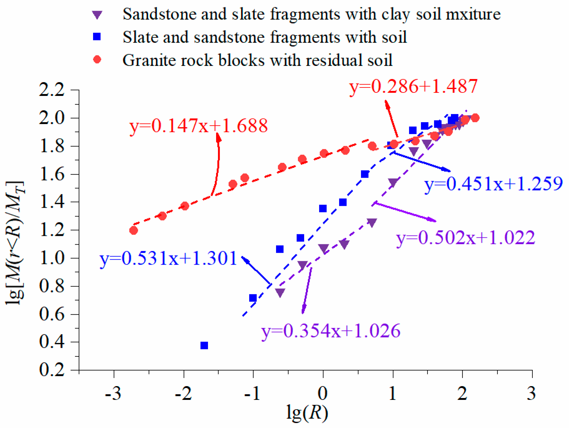
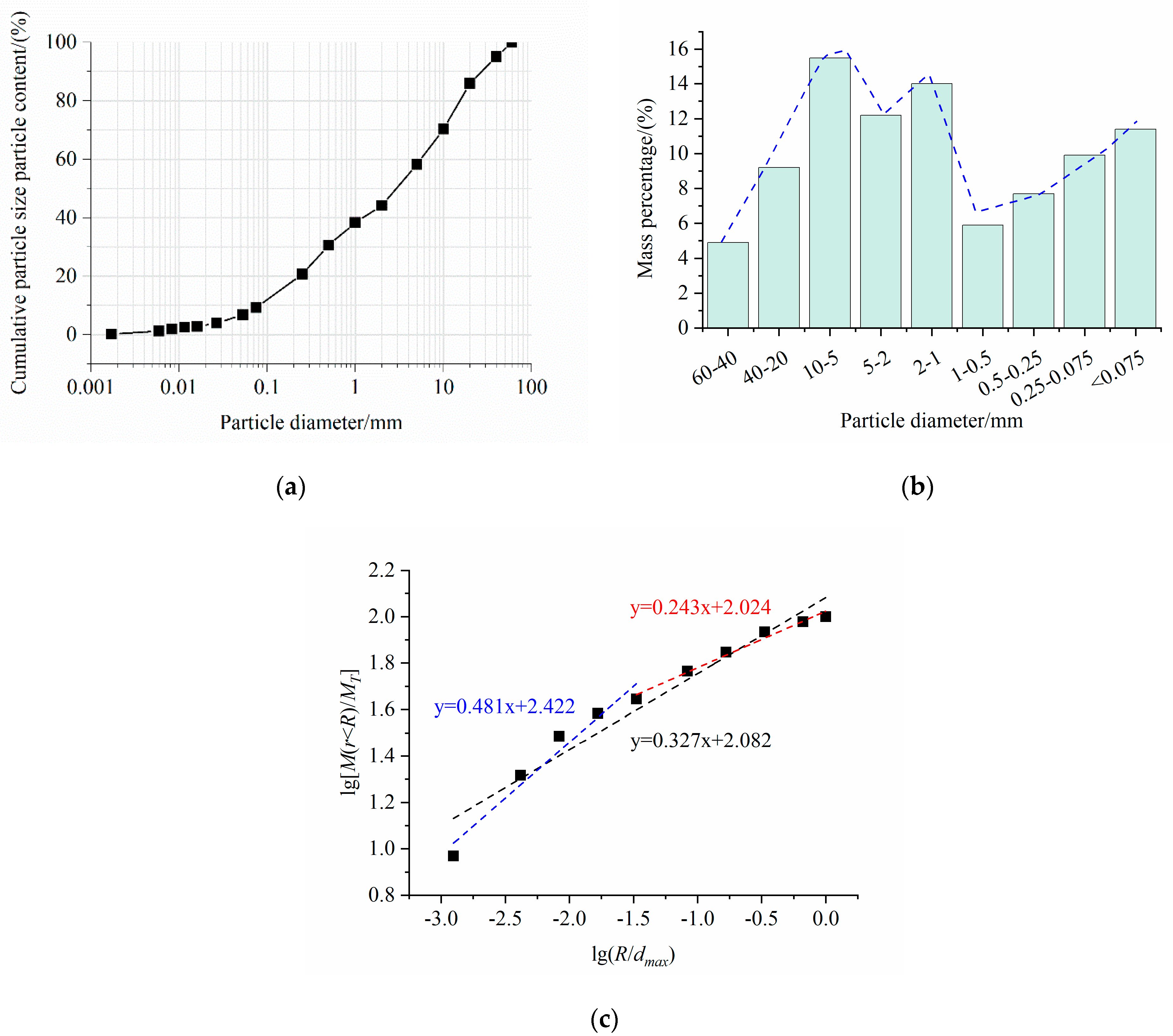
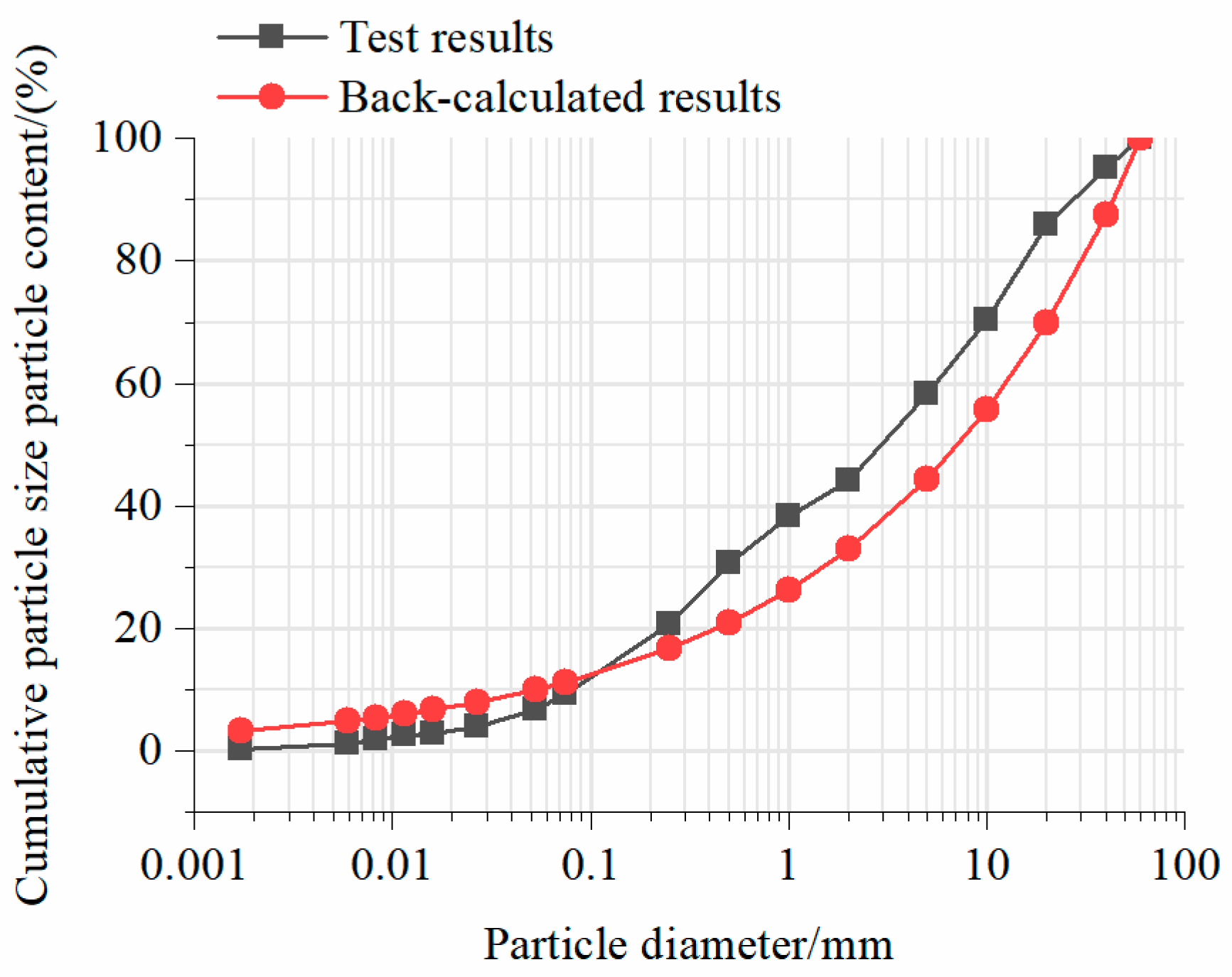
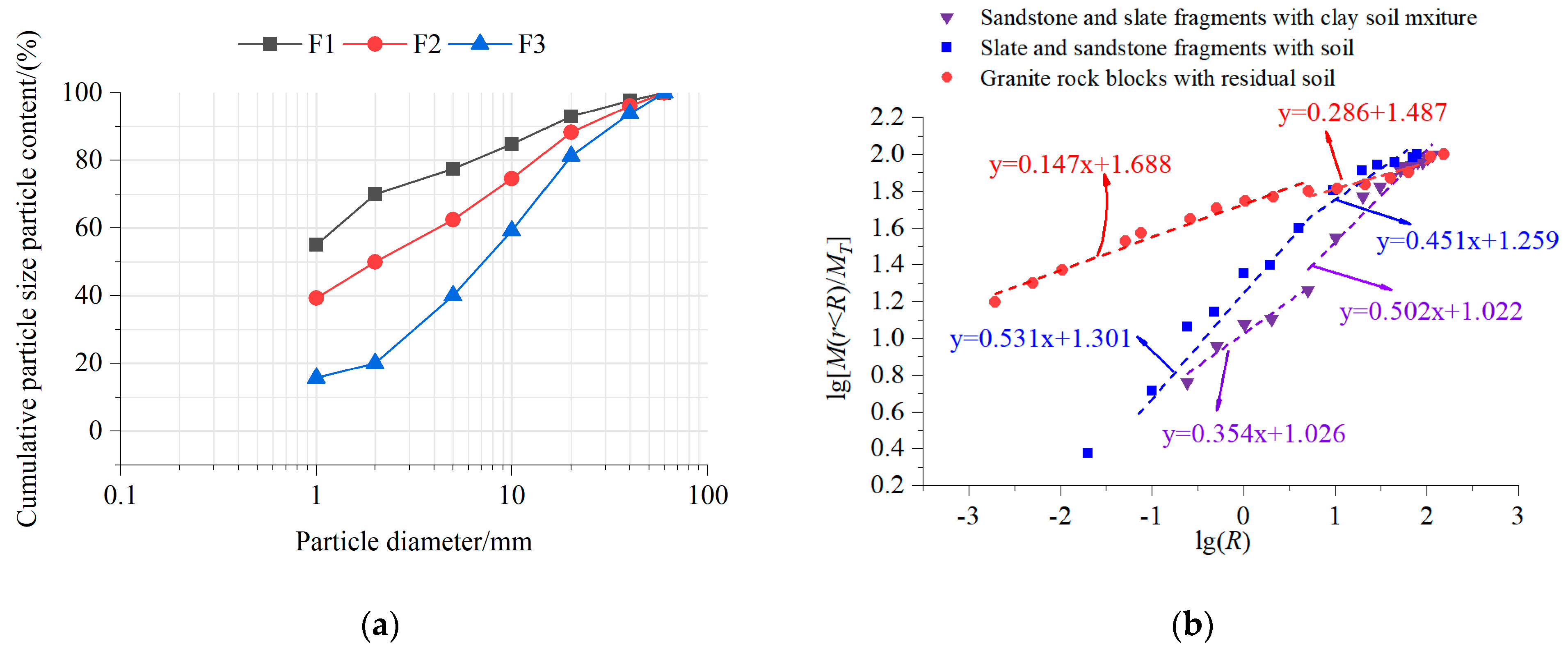
2.2. Fractal Characteristics of Soil–Rock Mixture

Several groups of S–RM samples have been collected from southwestern and southern China to figure out the fractal characteristic of S–RM, and the detailed information is listed in Table 1, and the distribution histogram of the fraction dimension is shown in Figure 4. The average fraction dimensions in Table 1 are in the range of 2.328~2.864, and most fractal dimensions fall into the 2.6~2.65 interval, followed by a distribution in the 2.65~2.70 interval.
Three typical fractal curves and the corresponding fractal dimensions of the representative S–RM are shown in Figure 5. The results show that the natural S–RM with different particle size distributions presents various fractal characteristics, and the particle content and size are basically linearly distributed under the double logarithmic coordinate system. The slopes of the fractal curves of these three samples present the evident difference as lg(R) increases. Taking the fractal curve of the mixture composed of the sandstone and slate fragments with the clay soil from [28] as an illustration. The slope of the fractal curve is 0.354 when the logarithm of the particle size is less than 0.75, and as the particle size increases, the value increases to 0.502 eventually. Correspondingly, the fractal dimension of the particle size reaches 2.646 for particle sizes under 5 mm and decreases to 2.498 for the particle size beyond 5 mm. The double fractal characteristic can be obtained based on the fractal curves of the S–RM with a good grading, which is quite different from that of the homogeneous soil.
Natural S–RM is a typical heterogeneous material which contains coarse grains with different sizes and contents. The fractional structure of S–RM is similar to that of the Menger Sponge model, and the formation process of S–RM can be considered as a construction process of Menger Sponge that is repeated an infinite number of times: the coarse grains with different sizes gradually substitute the same volume of the fine grain with the number of construction repetitions increases and finally form the S–RM with a certain particle size distribution. The difference in the particle size of the coarse and fine grains is more obvious according to the double fractal characteristics, and the particle size corresponding to the dividing point of the two fractal curves can be served as the coarse–fine grain threshold. On the one hand, the special double fractal characteristic illustrates the multiphase composition characteristics of S–RM; on the other hand, it effectively reflects the anisotropy due to the excessive difference in particle size. However, at the current stage of research, most researchers ignore the unique double fractal characteristics of S–RM and choose the average fractal dimension to describe the particle size distribution of S–RM, which leads to a certain degree of error, especially when describing the fractal structure of S–RM with the large difference in particle size and low rock content.

3. Material and Method
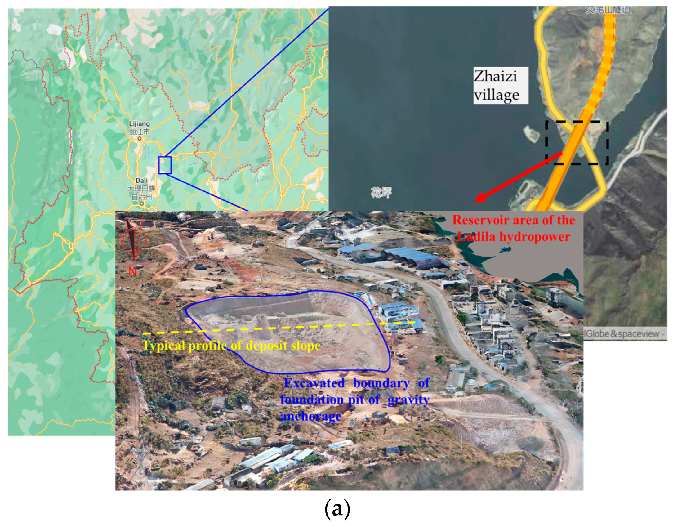
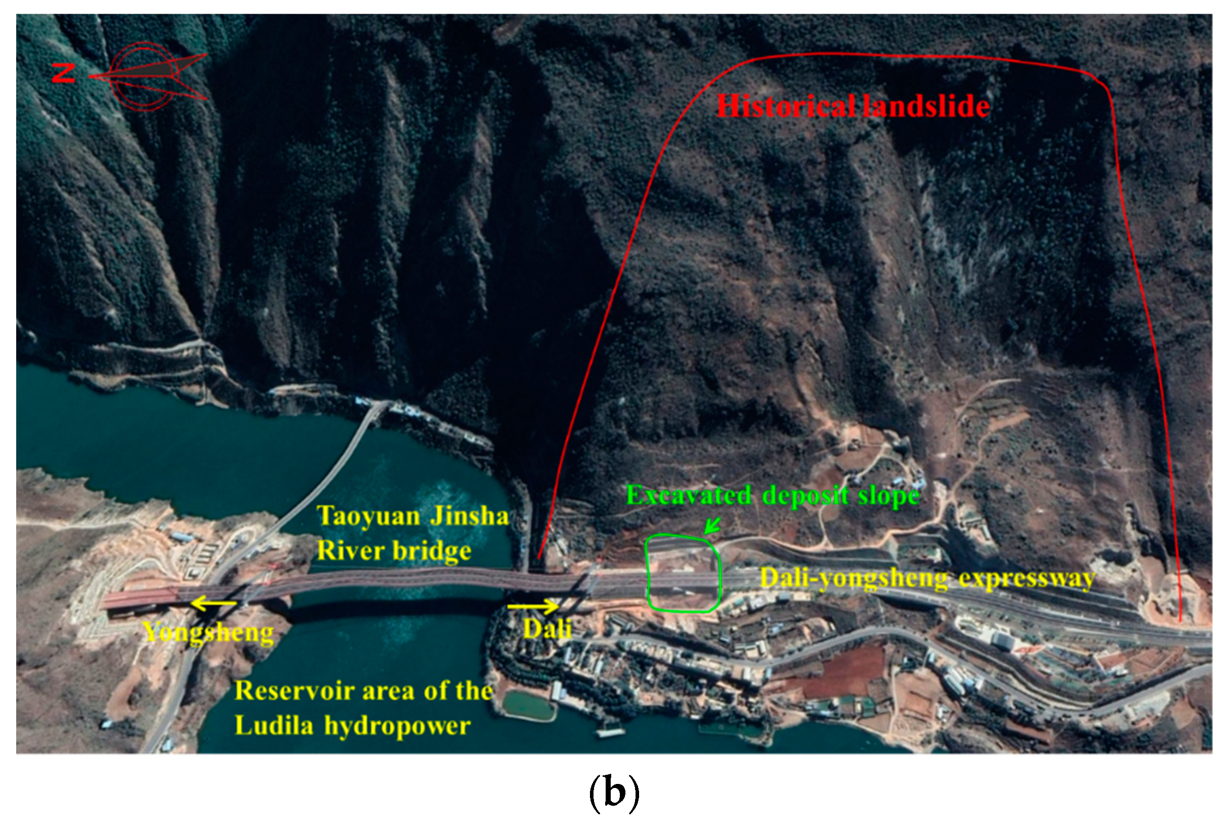
3.1. Study Area

The S–RM material utilized for the laboratory test is collected from the excavated deposit slope located near the Taoyuan Jinsha River bridge site in Yunnan Province, China (Figure 6a). The bridge site is located in the Jinsha River dry heat zone, which belongs to the low latitude plateau climate in the central subtropics. The seasonal distribution of precipitation is extremely uneven, showing a more obvious pattern of wet and dry with no rain and light rain as the main types of rainfall and heavy rain as the local extreme rainfall weather. Under the effect of the strong rainfall in the rainy season, the surface geotechnical has been strongly weathered. According to the geological survey and drilling hole results, the stratum lithology and geological structure of the excavated deposit slope are complex, and three engineering geological layers are divided based on the stratum lithology considering the engineering characteristics and engineering mechanical properties. The surface layer of the deposit slope is composed of the Quaternary Holocene colluvium, mainly composed of silt clay, breccia soil, and gravel soils, with different particle sizes of the rock blocks in the angular–subangular shape. The main component of the rock blocks is limestone, and the diameter range of the rock blocks is 2~6 cm. The large, isolated rock blocks with a diameter of 10 cm or more are scattered and distributed inside the excavated deposit slope. The underlying stratum of Quaternary Pleistocene alluvium is dominated by silty clay and silt in the medium dense–dense state. The third layer is Devonian medium–weathering limestone interspersed with muddy limestone, and the rock layer is relatively broken. The rock mass is mostly in the form of angular gravel crushed stone fracture structure and crushed stone crushed block mosaic structure. The buried depth of the groundwater is large, and the groundwater of the study area is 30~50 m below.

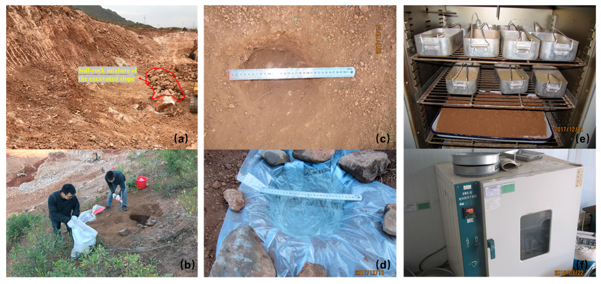
3.2. Material Sampling and Analysis

S–RM material for the physical and laboratory test was collected from the east surface region of the excavated deposit slope on the east side of the bridge anchor as shown in Figure 7a,b. The in situ density and water content were measured according to the relevant standard specified by the ‘Standard for Geotechnical Test Methods (GB/T 50123−2019)’. The in situ density test of the S–RM material was conducted with the water–filling method as shown in Figure 7c,d. First, the ground at the measurement point was leveled and checked with a level; after that, the size of the test pit will be determined according to the specification (Figure 7c), and the needed depth was dug. The representative specimen is used to calculate the moisture content once the sample from the pit is taken, weighed, and collected. The plastic film, which is larger than the volume of the test pit, was put along the bottom of the pit and the wall of the pit close to each other after the pit was dug and the corresponding size of the ring was set. Finally, the water in the storage cylinder was slowly injected into the plastic film (Figure 7d). When the water surface approaches the edge of the ground, the water flow was adjusted. After stopping the water injection for three to five minutes, the height of the water was measured level before and after the storage cylinder experiment. The water content of all samples used in the in situ density test was conducted with the help of the test apparatus of the Site Project Department of Yunnan Yunling Expressway Construction Group, and the test process is also shown in Figure 7e,f. The results indicate that the in situ density of the S–RM sample is 1500–2000 kg/m3, and the in situ water content is about 1.8~2.8%.
The particle size distribution of the S–RM sample was obtained based on the laboratory sieving test, and the cumulative distribution curve of the material collected from the east deposit slope is shown in Figure 8a. The coefficient of curvature (Cc) and coefficient of uniformity (Cu) were utilized to describe the particle size distribution characteristics from a quantitative perspective, and the calculation equations are as follows.
C u = d 60 d 10
C c = d 30 2 d 10 d 60
where d10, d30, and d60 are the equivalent to the particle size with 10%, 30%, and 60% cumulative content, respectively; d10 is the effective size; d60 is the control grain size.
The Cc and Cu of the S–RM material are 0.48 and 56.82, respectively, and the values indicate that the particle grading of the material in this area is discontinuous, and the overall gradation is poor. The histogram of particle size distribution as shown in Figure 8b shows that the distribution of each particle size of the S–RM in this area has obvious bimodality, and a significant decrease in the mass content can be found in the particle size range of 0.5~1 mm.
The fractal curve under the double logarithmic coordinates in Figure 8c presents an obvious segmentation feature, which indicates the S–RM material has an obvious double fractal characteristic. The slope of the fitting curve changes obviously when the particle size is 2 mm, which means the fractal characteristic of the particle larger than 2 mm and smaller than 2 mm is different. In combination with the histogram of particle size distribution and particle size distribution characteristics, the coarse–fine threshold of the S–RM material can be set as 2 mm. The particle larger than 2 mm can be considered as the generalized rock block, and the particle smaller than 2 mm can be considered as the generalized soil matrix. The rock block proportion (RBP) of the natural S–RM is calculated as 61.68% according to the particle size distribution grading curve. According to Equation (7), the fractal dimension D of the material can be obtained by taking the logarithm on both sides as follows.
D = 3 ln M ( r < R ) M T ln R d max
The fractal dimensions of the fine (Ds) and coarse grain (DR) are 2.489 and 2.713, respectively, and the average fractal dimension (Dave) is 2.633.

3.3. Experimental Scheme

The discussions above about the fractal characteristics show that the double fractal characteristic of the S–RM material in the study area can be observed, and the difference in the fractal dimension of the rock blocks and soil matrix is significant. The back–calculated particle size grading curve obtained using Equation (7) and the average fractal dimension are shown in Figure 9. The obvious difference between the back–calculated and measured particle size grading curve shows that the irrationality of using the average fractal dimension to describe the particle distribution characteristic of S–RM. In order to reveal the influence of double fractal characteristic on the mechanical behaviors of S–RM, the S–RM samples with different fractal characteristics were prepared based on different fractal characteristics and particle size distributions as shown in Figure 10. The fractal dimensions of the soil matrix and rock block and the average values of three test samples are listed in Table 2. The large–scale three triaxial unconsolidated undrained tests were carried out to investigate the mechanical behaviors of S–RM. The sample size was set as with a diameter of 300 mm and height of 600 mm, and the dmax value of the S–RM specimen is 60 mm. The dry S–RM material was sieved in accordance with the designed particle grading, and the required mass of water for the specimen was calculated according to the in situ natural water content. Then dry material was mixed with the natural water content uniformly. The mixed material was put into the apparatus by layers with compaction and gouging, and the mixed sample was placed in a closed container and left to stand for 24 h. The confining pressure was set as 200, 300, 400, and 600 kPa, and the test was stopped when the axial strain reaches 15%.

3.4. Analysis Method

Discussions about the strength characteristic of S–RM in the previous studies are primarily divided into two types, one for the linear strength characteristic and one for the nonlinear strength characteristic. Linear strength characteristic is described based on the Mohr–Coulomb law, and the cohesion (c) and friction angle (φ) are two key indexes to evaluate the shear strength of S–RM. However, some S–RM triaxial test results show that the shear stress presents a continuously increasing trend with the axial strain, and the strain–hardening effect is obvious. The hyperbolic feature of the stress–strain curve is much more apparent with a higher rock content and confining pressure. The curve of the strength envelop gradually shows a nonlinear trend with the increase in normal stress, which also leads to the constantly changing peak friction angle with the normal stress. A hyperbolic fitting equation was proposed by Duncan and Chang [45] based on the triaxial test results of remolded soil named after the Duncan–Chang model, which is known as a nonlinear elasticity model based on the incremental generalized Hooke’s law. The expression of the Duncan–Chang model is as follows.
σ 1 σ 3 = ε 1 a + b ε 1
where σ1 and σ3 are the measured first and third principal stress during the test, and ε1 is the axial strain.
When the axial strain tends to be infinitesimal, the initial elastic modulus at the starting point of the test can be calculated as follows.
E i = σ 1 σ 3 ε 1 ε 1 0 = 1 a
where Ei is the initial elastic modulus.
When the axial strain tends to be infinite, the ultimate deviatoric stress can be obtained as follows.
σ u l t = σ 1 σ 3 u l t = 1 b
where σult is the ultimate deviatoric stress.
In fact, the axial strain cannot reach infinity during the test, and the peak strength (σ1σ3)f can be determined based on the test or fitting results, with the help of the hyperbolic equation as shown in Equation (12) or the linear strength indexes (c and φ). The failure ratio Rf can be obtained based on the ultimate deviatoric stress and peak strength as follows.
R f = σ 1 σ 3 f σ 1 σ 3 u l t
The test constants a and b can be obtained by the fitting curves of ε1/(σ1σ3) and ε1, and the value of the initial elastic modulus and ultimate deviatoric stress can be determined.
Janbu [46] suggested a calculation relationship between the initial elastic modulus and confining pressure in the power form to describe the positive influence of confining pressure as follows.
E i = K P a σ 3 P a n
where K and n are test constants to inflect the influence of confining pressure on the initial elastic modulus.
The tangential elastic modulus in the Eμ model can be described as follows.
E t = K P a σ 3 P a n 1 R f σ 1 σ 3 1 sin φ 2 c cos φ + 2 σ 3 sin φ 2

4. Results and Discussion

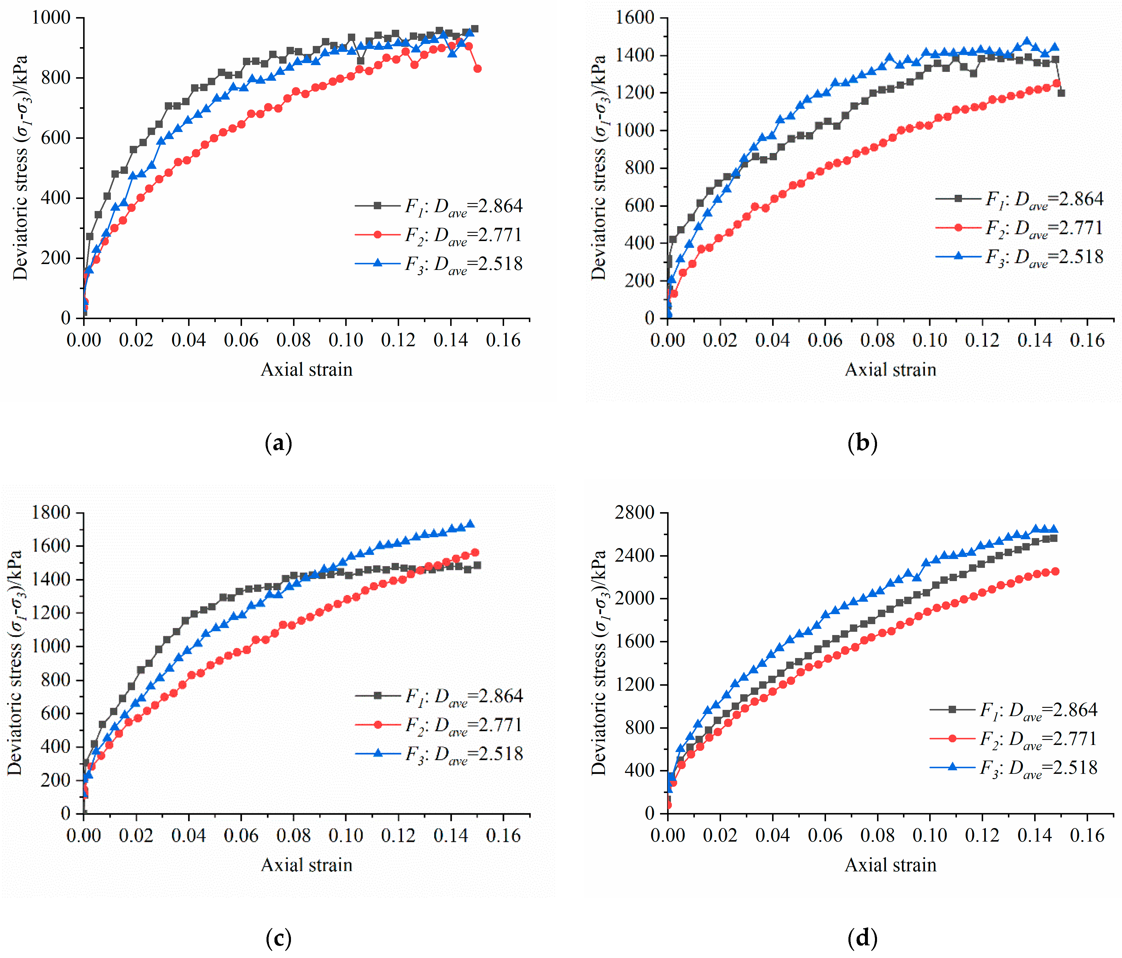
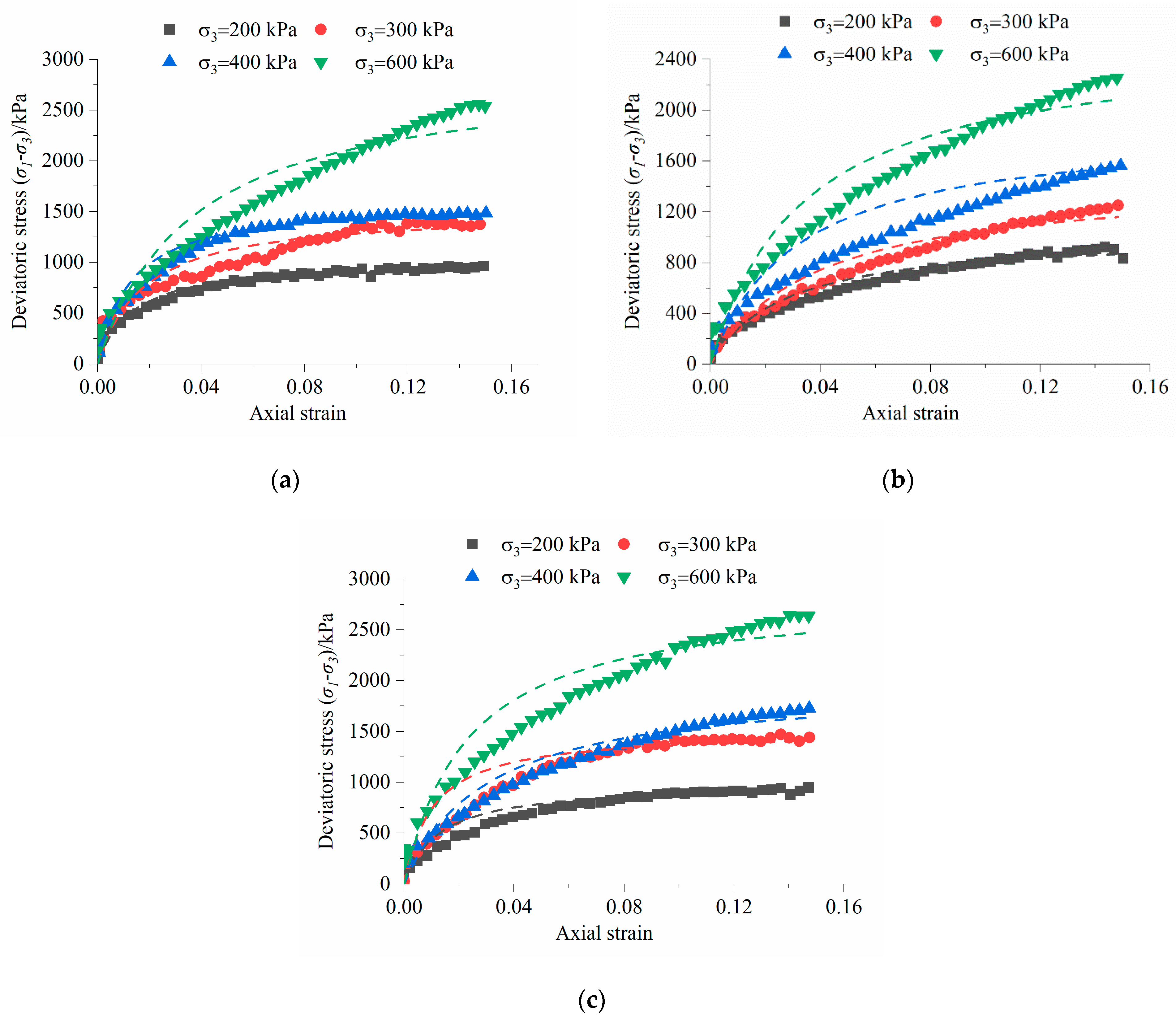
4.1. Analysis of Deviatoric Stress–Axial Strain Curve Characteristics

The curves of the deviatoric stress (σ1σ3) and axial strain of S–RM samples with different fractal dimensions under different confining pressure are shown in Figure 11. The results show that the deviatoric stress presents a nonlinear increasing trend with axial strain, and the curves of the deviatoric stress–axial strain of sample with different fractal dimensions are similarly presented in the hyperbolic shape. As shown in Figure 11, the deviatoric stress increases with axial strain in a linear trend at the initial state and the difference in the increasing rates of the deviatoric stress affected by the fractal characteristic gradually appears as the axial strain increases. Compared to the similar stress values after the axial strain greater than 0.08 in Figure 11a,b, the difference in the stress values among the three samples is much more obvious as the compressive stress increases. The slopes of the stress–strain curves of the F1 and F3 samples both present a trend of increasing and then decreasing as shown in Figure 11a,b, and the values of the deviatoric stress of the three samples are close at the final under the low compressive stress conditions. The difference in the stress–strain curve and increasing trend of the deviatoric stress of samples with different fractal characteristics become more apparent as the confining pressure increases. The deviatoric stress of the F2 and F3 samples shows a continuously increasing variation with axial strain under 400 kPa confining pressure conditions as shown in Figure 11c. The strain−hardening effect is obvious in all these three samples when the test was carried out under a high confining pressure condition. Slight fluctuations can be observed in the curve under the confining pressure condition of 200 kPa (Figure 11a), while the curve is relatively smooth when the confining pressure is 600 kPa (Figure 11d). It is attributed to the low possibility of the rock block breakage inside the sample under the low confining pressure conditions, and the extension and destruction of the shear face are obstructed by the rock block, resulting in fluctuations of the deviatoric stress.
Most of the deviatoric stress–axial strain curves in Figure 11 are in the hyperbolic shape, and no significant peak strength and stress drop effect was found. Therefore, the deviatoric stress corresponding to 15% axial strain is set as the maximum deviatoric stress in this study. The maximum deviatoric stress of the S–RM with different fractal dimensions and confining pressure is listed in Table 3. The results in Figure 12a show that the confining pressure plays a positive role in the maximum deviatoric stress and the difference in the maximum deviatoric stress of the sample with different fractal dimensions is much more obvious with the confining pressure, which means that the strength of S–RM is more sensitive to the fractal characteristic under a higher confining pressure condition. The maximum deviatoric stress values of the samples under 200 kPa are in the range of 920.02~962.49 kPa, and the fractal characteristic presents less impact on the strength. As the confining pressure increases, the differences in the strength become much more evident. The maximum deviatoric stress of the F1 and F3 samples with Dave = 2.864 and 2.518 are approximate, which is basically higher than that of the F2 sample with Dave =2.771, except for the confining pressure of 400 kPa. When the confining pressure reaches 600 kPa, the maximum deviatoric stress of three samples has been greater than 2000 kPa, and the difference in the strength of S–RM samples with different fractal characteristics has reached 387.83 kPa. Figure 12b shows that the parabolic shape changes in the shear strength of reduction followed by an increase with fractal dimension can be found under 300 kPa and 600 kPa compressive circumstances. The schematic of the sample with different fractal dimensions in Figure 3 shows that variation in the fractal dimension results in different structural characteristics and the change of the source of the whole material strength. The fine grains in the F1 sample, which has a larger fractal dimension, can still provide a greater cohesive effect for the material, while the contact friction between the coarse grain in the F3 sample is mostly essential for the overall strength of the material. The strength source is more complicated for the F2 sample with the cooperation of the coarse and fine grain particles, displaying a relatively abnormal decline. The discussions above indicate that the shear strength of S–RM exhibits a clear response as the fractal dimension changes, and the fractal dimension can be used as a link between the structural features and mechanical properties of S–RM.

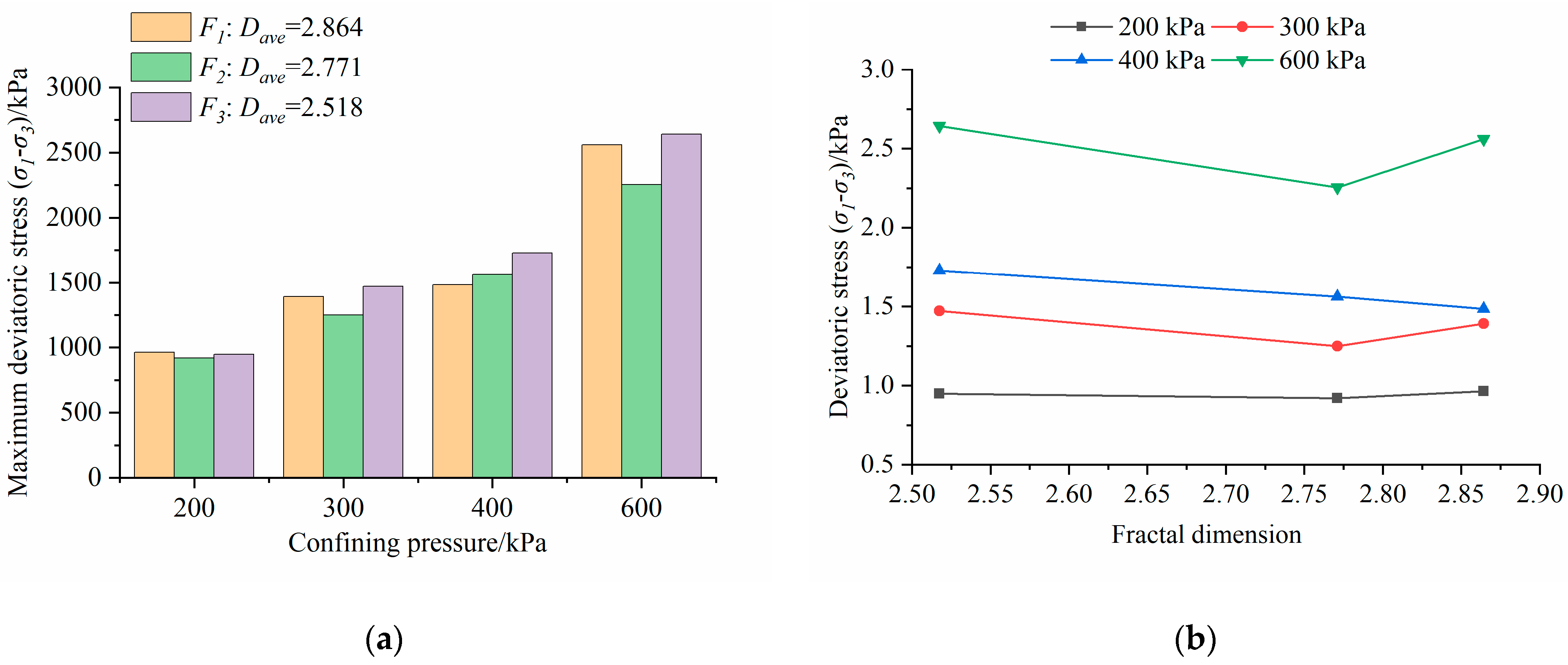
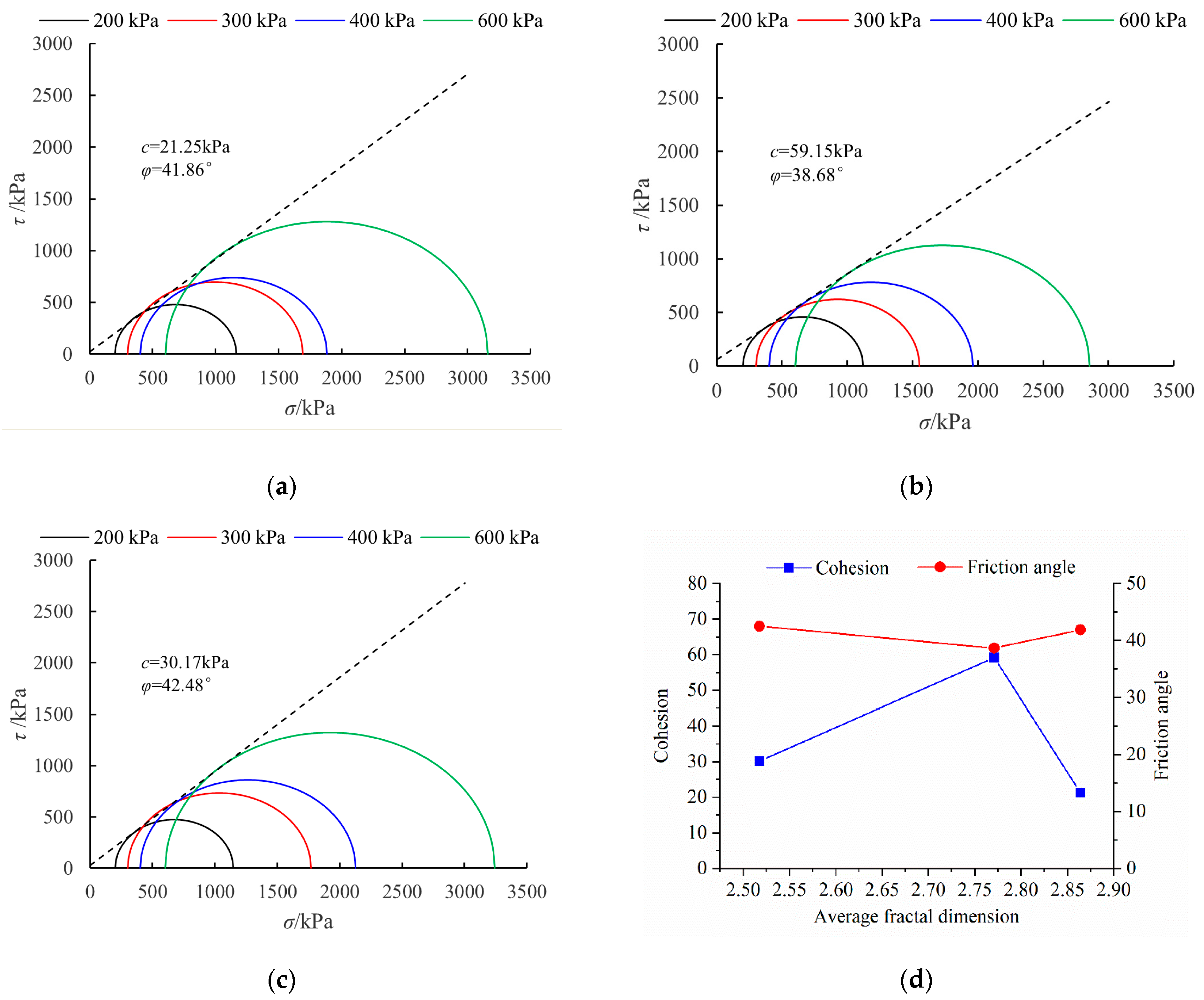
4.2. Analysis of Linear Strength Index Characteristics

Cohesion and friction angle are the most widely used linear strength indexes to evaluate the shear strength of the geotechnical material, of which the accuracy and availability have been verified in previous studies. The failure envelopes and the corresponding cohesion and friction angle values of S–RM with different fractal characteristics are obtained using the Mohr–Coulomb strength criterion based on the experimental data are shown in Figure 13. The results show that the cohesion of S–RM presents an increasing and then decreasing trend with average fractal dimension, and the cohesion of F2 sample is the greatest as 59.15 kPa. The maximum and minimum cohesion difference is about 30.2 kPa. The variation of friction angle of the sample with different fractal characteristics is less pronounced and the value is in the range of 38.68°~42.48°. The variations of the linear strength indexes of the F1 and F3 samples are both not related to the fractal dimension, especially the value of the friction angle.
The impact factors on the strength indexes of the granular material are various, such as material composition, particle arrangement, component content, etc. Previous studies have revealed that the fine and coarse grain in S–RM present quite different particle size distributions, and the suitable particle size distribution can allow the fine grain to fill the voids between the rock blocks well, leading to a higher macroscopic cohesion [47,48,49,50]. In this study, the fractal curves show that the continuity of the fractal dimension of the F2 sample is the best and the fractal dimensions of the fine and grain coarse are the closest, which means that the linear fractal characteristic is the most obvious. The sufficient mixing of the fine and coarse grain leads to a well–filled S–RM sample under this condition and increases the difficulty when the soil–rock interface is damaged, which results in the highest cohesion of the F2 sample. Compared to the friction angle of the F2 sample, there is an evident increase in the friction angle of the F3 sample. According to the particle size distribution, the decrease in the fractal dimension of the F3 sample presents a higher non–homogeneity in the particle size distribution, resulting in a higher rock content. As rock content increases, the randomly distributed rock blocks come into contact with each other, and the friction and occlusion effect play a major role in the increasing macroscopic friction angle.

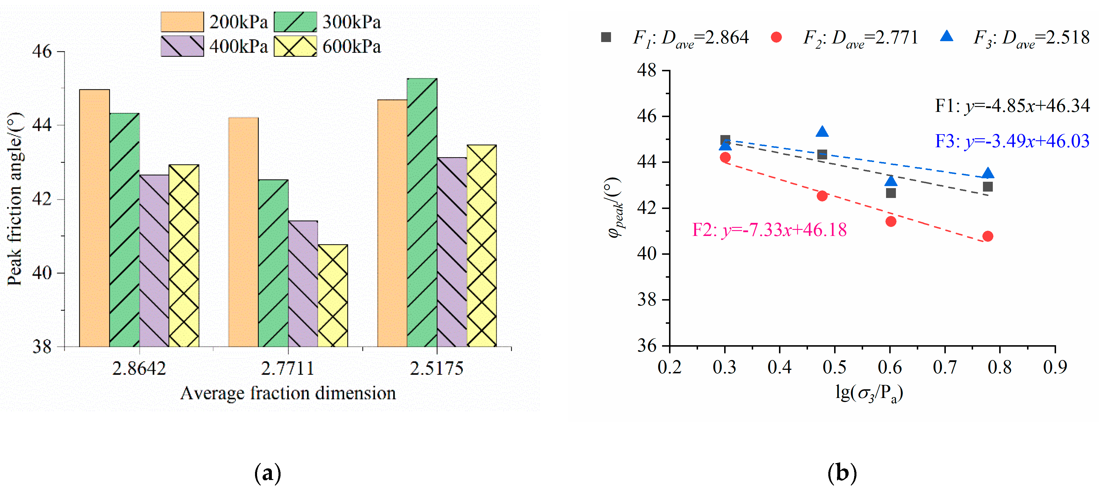
4.3. Analysis of Nonlinear Strength Index Characteristics

The strength envelopes of F1 and F3 samples in Figure 13a,c both present a relatively obvious nonlinear trend, and the slope of the curve is not constant. The peak friction angle is proposed to describe the nonlinear characteristic of the strength of S–RM as follows under the assumption that the cohesion of the material is zero.
φ p e a k = arcsin σ 1 f σ 3 f σ 1 f + σ 3 f
where φpeak is the peak friction angle; σ1f and σ3f are the measured first and third principal stress at the failure stage of the test.
The φpeak values of the S–RM with different Dave values under various confining pressure are shown in Figure 14a. The results show that the influence of fractal characteristics on the φpeak values is related to the confining pressure. Under the relatively low confining pressure of 200 kPa, the φpeak values of three samples are close to 44.5°. The obvious positive influence of the fractal dimension on the φpeak value can be observed when the confining pressure is between 400 kPa and 600 kPa.
The relationships between the peak friction angle and confining pressure of S–RM with different fractal characteristics are shown in Figure 14b. The results show that the peak friction angle decreases with the confining pressure, and the linear relationship can be observed between the friction angle and logarithmically processed confining pressure as follows.
φ p e a k = φ 0 Δ φ lg σ 3 P a
where φ0 is the internal friction angle when the confining pressure is the atmospheric pressure; Δφ0 is utilized to describe the decrease in the friction angle with different confining pressure; Pa is the atmospheric pressure.
The Δφ0 and φ0 values of the S–RM with different Dave values under different confining pressure are shown in Figure 13b. As Dave decreases from 2.864 to 2.771, the Δφ0 presents an obvious increase from 4.85 to 7.33, and the value drops back down to 3.49 as Dave decreases. It is found that the value of φ0 shows a decreasing trend as Dave increases; however, the value remains around 46° overall.
As shown in Equation (19), the φpeak value is obtained based on the assumption that the cohesion of the material is equal to zero, and φ0 can be considered as the macroscopic representation of the cohesive effect and frictional interactions of the components. The appearance of the rock block leads to a more complex and heterogeneous structure of S–RM with a lower fractal dimension compared with that of the pure soil matrix sample. The decreasing trend of the φ0 value as the Dave value increases shows that the relatively homogeneous particle size distribution with a higher Dave value contributes to more effective interaction between the components inside S–RM.
The parameters in Duncan–Chang model are analyzed using Equations (12)–(17), and the fitting curves of deviatoric stress–axial strain using the hyperbolic equation are shown in Figure 15. The results indicate that the stress–strain test curves present an obvious increasing trend, and the shape of the curves is hyperbolic. The stress–strain fitting curves of S–RM under 200 and 400 kPa confining pressure are close to the test curves, and the difference between the test and fitting curves appears as the confining pressure increases.
The initial elastic modulus (Ei) of S–RM mainly presents a complex variation trend with confining pressure as shown in Figure 16. The Ei value of the F1 sample with Dave = 2.864 suddenly decreases from 127.89 MPa to 79.29 MPa when the confining pressure increases from 400 kPa to 600 kPa. The test results of the F2 sample with Dave = 2.771 show a relatively significant positive influence of the confining pressure on the Ei value. The sudden decrease can be observed in the F3 sample with Dave = 2.518 as the confining pressure increases from 300 kPa to 400 kPa. However, compared to the value at 200 kPa, an increase in Ei value still can be obtained at 600 kPa. A similar increase can also be observed in the initial elastic modulus of the F2 sample. The Ei value of the F2 sample at 600 kPa confining pressure is about 1.93 times the value at 200 kPa, while the ratio is about 2.718 for the F3 sample. For the F1 sample with Dave = 2.864, the Ei value remains in the range of 75–85 MPa except for the value corresponding to the confining pressure of 400 kPa. It seems that the variation of the initial elastic modulus is related to the fractal characteristic, and the Ei value of the sample with a higher degree of non–homogeneity and rock content presents more sensitivity to the confining pressure, and the corresponding Ei value is also much higher.
According to Equation (16), the initial elastic modulus presents a power−increasing trend with confining pressure in the D−C model. The scatter plot of logarithmic Ei values with different confining pressure is shown in Figure 17, and the parameters K and n can be obtained based on the fitting curve of log10(Ei/Pa) and log10(σ3/Pa). The results show that the linear relationships between the log10(Ei/Pa) and log10(σ3/Pa) of F1 and F3 samples are not obvious, and the sudden decreases in log10(Ei/Pa) can be observed at σ3 = 400 kPa and 600 kPa. The better linear fitting curve can be found in F2 sample Dave = 2.771 with R2 larger than 0.85. The hyperbolic fitting curves of deviatoric stress–axial strain in Figure 15 indicate that the errors in the slope of the fitting and test curves are obvious under the conditions of confining pressure at 400 kPa and 600 kPa.
The secant modulus of geotechnical material is a key deformation parameter to describe the average stiffness, which is commonly obtained using the uniaxial compressive test. Duncan and Chang [43] pointed out that the secant modulus corresponding to the 50% peak strength, E0.5, is an important parameter in the D−C model, and the value is determined based on the slope of the line between the stress corresponding to 50% of uniaxial compressive strength and the original on the stress–strain curve. The E0.5 values of S–RM samples with different fractal dimensions under different confining pressure conditions are shown in Figure 18. The results show that the E0.5 value presents an obvious increasing trend with the confining pressure under the fractal dimension of F2 and F3 samples, while values of F1 sample seem to be less related to the confining pressure variations. The F1 sample with Dave = 2.864 presents the maximum average E0.5 value of 37.99 MPa, which is about 1.83 times the E0.5 value of the F2 sample with Dave = 2.711. The decrease in the fractal dimension increases the difference in the E0.5 value, and the stiffness of the material under the higher confining pressure is much larger.
The numerical particle models of the three samples in Figure 3 show that the spatial distribution of the rock block is related to the fractal characteristic. According to the particle grading curve, the fine grain (soil) content of F1F3 samples is 70%, 50%, and 20%, respectively. Figure 3a presents that most of the large−size rock particles in the F1 sample are randomly distributed inside the sample, and compared to the pure soil matrix, the integrity of the sample was damaged. The soil and small−size rock particles fill the voids formed between the large−size rock particles in the F2 sample, and both the soil and rock particles can play roles in affording the external force as shown in Figure 3b. However, as the rock content increases, the large−size rock particles are dominant component in the structure of the sample, and the obvious voids can be found between the large−size rock particles (Figure 3c). The structure characteristics of F3 sample has shown the evident different from that of the pure soil, and the inhomogeneity of the particle size inside the sample is more obvious.
Previous studies have indicated that the fractal dimension is related to the particle size distribution and the complex structure of the geotechnical material. According to Figure 10b, the difference in slope of the segmented and average fractal curves is relatively more pronounced in the F3 sample. The largest difference between the coarse and fine−grain fractal dimensions appears in the F3 sample with 0.239, and the smallest value appears in the F2 sample. The parameters in the D−C model discussed above show that only the stress–strain curve of the F2 sample presents a good fit to the hyperbolic stress–strain, while obvious errors between the fitting and test values of the F3 sample under the high confining pressure conditions can be observed. The relatively abnormal increase in the elastic modulus parameters appears in the F1 and F3 samples under different confining pressure. The difference in the fraction dimension of the rock block and soil matrix indicates that the duality in the particle size is nonnegligible in the F3 sample, and the component duality has a significant effect on the mechanical properties of S–RM.
The traditional D−C model was proposed to describe the nonlinear mechanical behaviors of the soil material based on the test results, and the model has been widely used in discussions about the earth and rock dam materials in recent years. However, there are still significant differences in the particle size distribution characteristics of the rockfill dam material and natural S–RM. The maximum particle diameter of the rockfill dam can generally reach more than 10 cm and has a relatively low fine grain content, which is commonly not exceeding 15%. The ability of rockfill material to resist the deformation caused by external force mainly comes from the friction and interlocking effect between the coarse particles. Instead, the cohesiveness of the fine grain and the strength of the coarse–fine interface both have a vital impact on the whole strength of S–RM. Therefore, the applicability of the traditional D−C model in describing the mechanical behaviors of S–RM with various particle size distributions still needs to be discussed.
In contrast to the use of conventional particle size distribution index, fractal dimension was chosen for this study. The fractal characteristics of the S–RM located in the southwest and southern regions of China were analyzed based on the previous studies, and the mechanical properties of S–RM with various dimensional characteristics using the material from a deposit slope in Yunnan, China, was discussed. Because the sampling sites and numbers are constrained, the obtained experimental results are relatively few, and more studies are still needed to figure out the spatial distribution characteristics of the fractal characteristics of the S–RM and the corresponding responses of the mechanical properties.

5. Conclusions

This study focused on the fractal characteristics of the natural S–RM and analyzed the impact of the fractal dimension on the mechanical behaviors of the S–RM collected from Yunnan, China, based on the large–scale triaxial test results. Several groups of the particle size distribution of the S–RM located in the Three Gorges Reservoir and southwest of China were first collected, and the fractal characteristics were analyzed. The impact of the fractal characteristics on the mechanical behaviors was then investigated using the S–RM located in the excavated deposit slope in Yunnan. The investigation of the linear and nonlinear strength indices of S–RM with various fractal qualities was followed by a discussion of the impact of the double fractal characteristics on the structure and mechanical properties. The main conclusions are as follows:
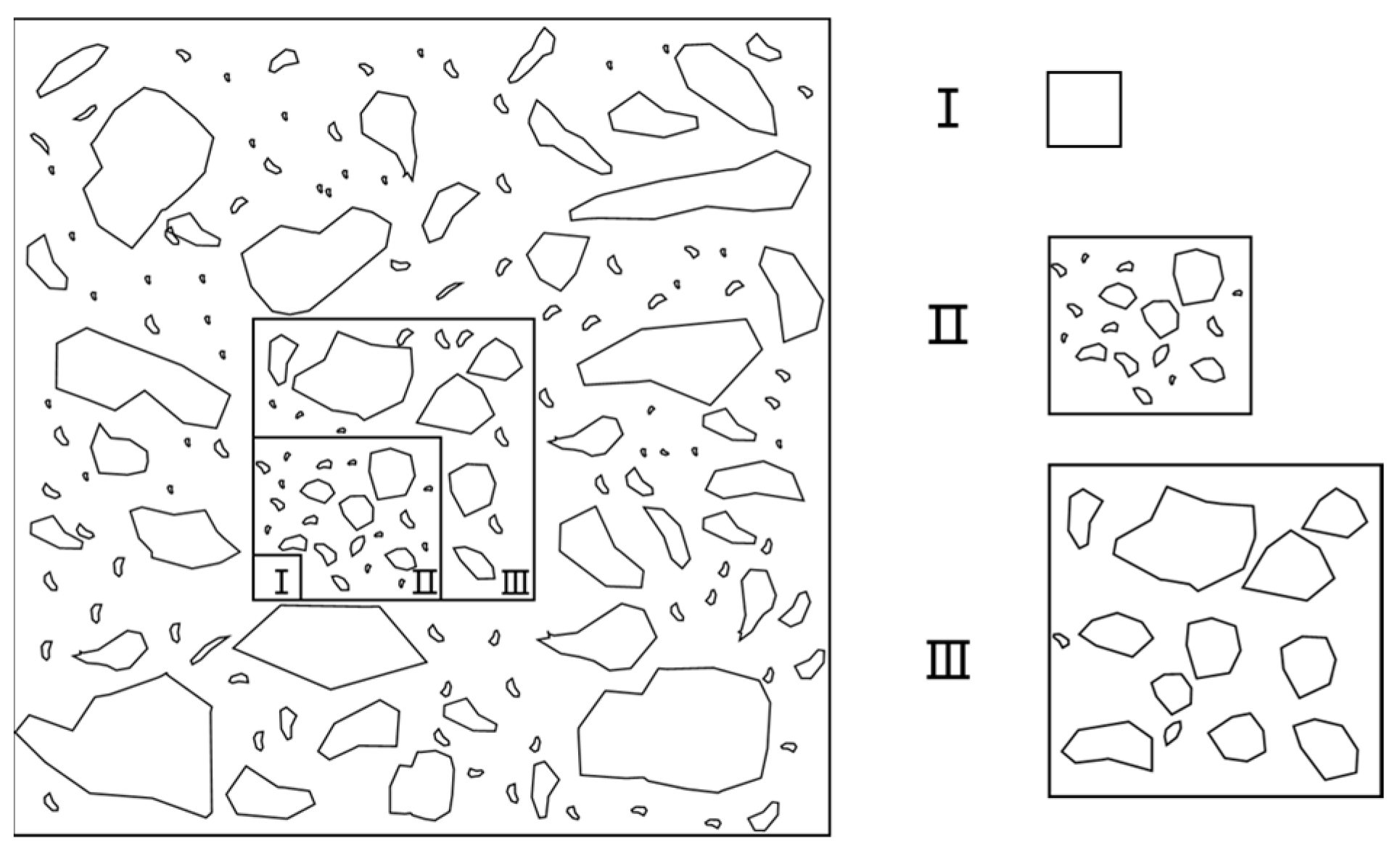
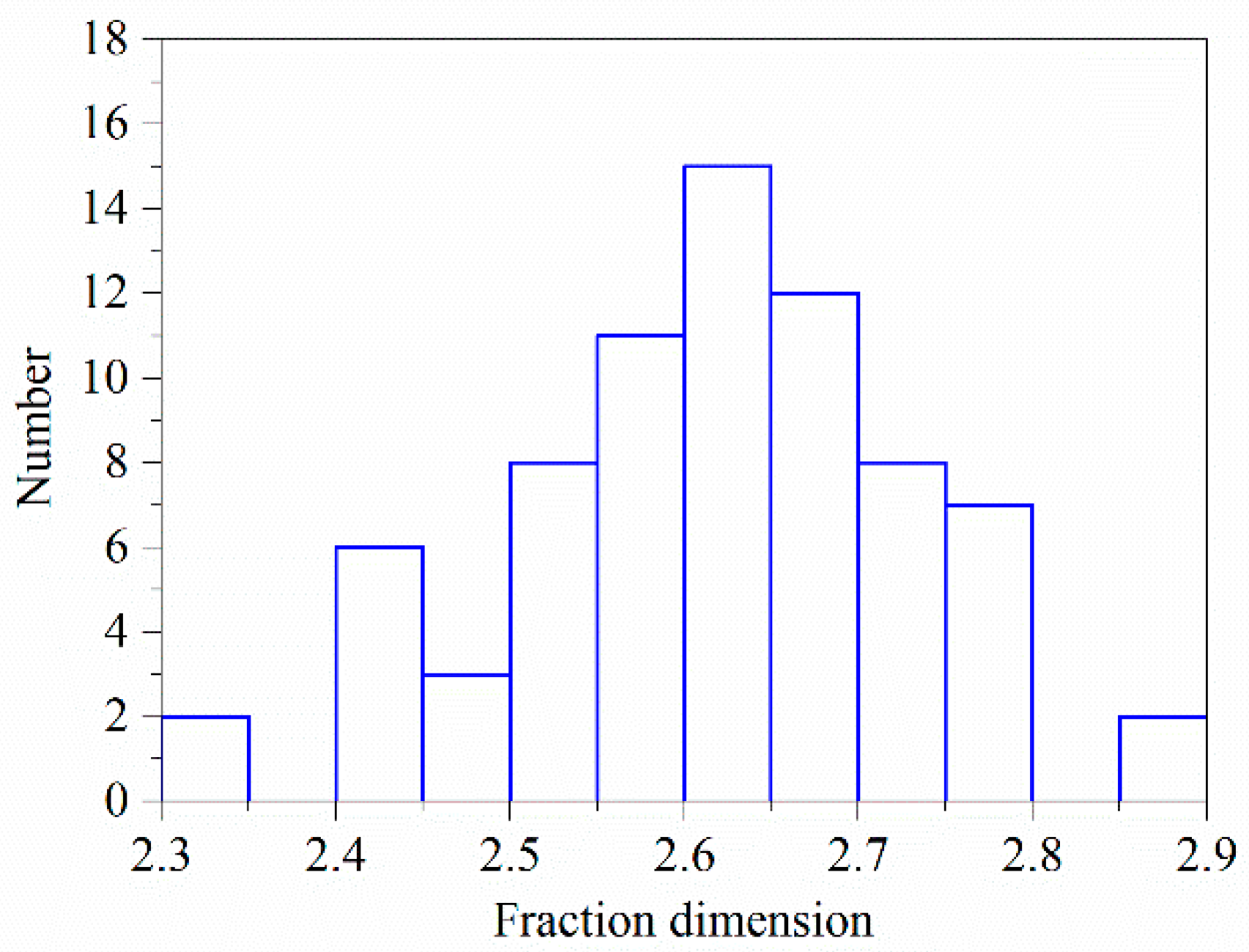
  • The majority of the particle size distributions of the natural S–RM in southwest China and Three Gorges Reservoir satisfy the fractal distribution. The average fractal dimension of the material ranges from 2.328 to 2.864. The double fractal characteristic of the material can be observed due to the difference in the particle size of the coarse and fine grain, and the particle size corresponding to the segments of the fractal curve can be thought of as the threshold diameter of the coarse and fine grain.
  • The large–scale triaxial test of S–RM with various fractal dimensions shows that the linear and nonlinear strength indexes are both affected by fractal characteristics. The cohesion presents an increasing and then decreasing pattern as the average fractal dimension increases, while the friction angle is mainly within the range of 38.68°~42.48°. The peak friction angle decreases from 46.34° to 46.02° as the average fractal dimension decreases from 2.864 to 2.518.
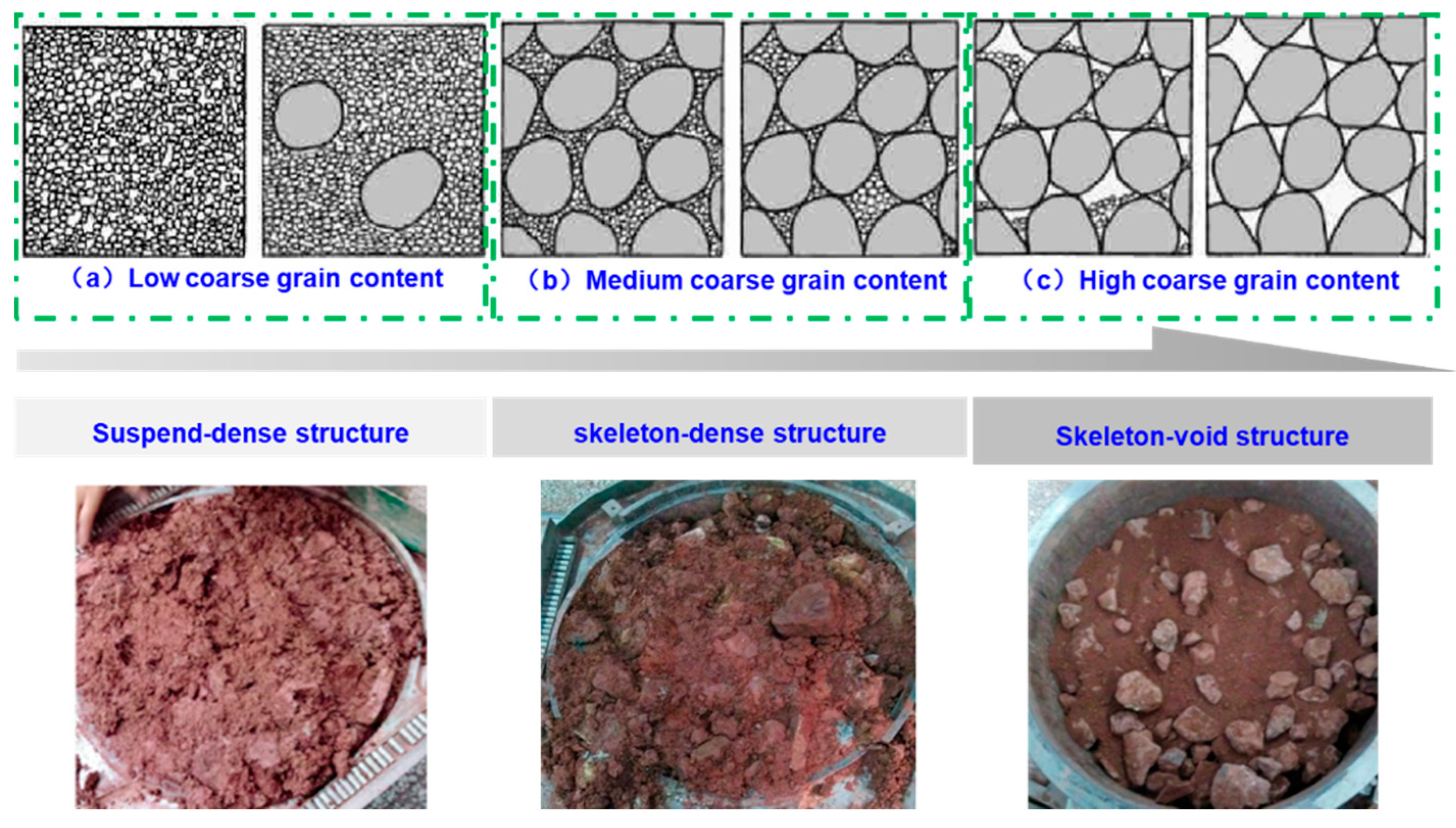
  • The results show that the difference in the fractal dimension of the coarse and fine grain becomes more pronounced as the coarse grain content increases, and the use of the average fractal dimension to study the mechanical properties would result in certain inaccuracies. The degree of the particle size inhomogeneity and the voids between the coarse grains both increase as the coarse grain content increases, and the contact friction effect between the coarse grain starts to play a role in the strength of the material. In this case, the duality of the S–RM due to the multi–phase component has a more evident influence and results in more complicated mechanical properties.

Author Contributions

Conceptualization, Z.Z. and X.F.; Methodology, Z.Z., W.Y. and Y.D.; Validation, Q.S. and W.Y.; Formal Analysis, W.Y. and Q.S.; Investigation, S.C.; Writing—Original Draft Preparation, Z.Z. and Q.S.; Writing—Review and Editing, X.F.; Visualization, Y.D. and S.C. All authors have read and agreed to the published version of the manuscript.

Funding

This work was supported by the Open Research Fund of the State Key Laboratory of Geomechanics and Geotechnical Engineering (Grant No. SKLGME021013), Open Research Fund of the State Key Laboratory of Geohazard Prevention and Geoenvironment Protection (Grant No. SKLGP2022K010), the Youth Innovation Promotion Association CAS (Grant No. 2021325), National Natural Science Foundation of China (Grant No. 52179117, 52209131), Key Laboratory of Roads and Railway Safety Control (Shijiazhuang Tiedao University), the Ministry of Education (STDTKF202103).

Institutional Review Board Statement

Not applicable.

Informed Consent Statement

Not applicable.

Data Availability Statement

The data are available from the corresponding author upon request.

Conflicts of Interest

The authors declare no conflict of interest.

References

  1. You, X.H. Stochastic structural model of the earth-rock aggregate and its applicaiton. Chin. J. Rock Mech. Eng. 2002, 21, 1748. [Google Scholar]
  2. Xu, W.J.; Hu, R.L. Conception, classification and significations of soil-rock mixture. Hydrogeol. Eng. Geol. 2009, 36, 50–56, 70. [Google Scholar]
  3. Wei, H.Z.; Wang, R.; Hu, M.J.; Zhao, H.; Xu, X.Y. Strength behaviour of gravelly soil with different coarse-grained contents in Jiangjiagou Ravine. Rock Soil Mech. 2008, 29, 48–51, 57. [Google Scholar]
  4. Kalender, A.; Sonmez, H.; Medley, E.; Tunusluoglu, C.; Kasapoglu, K.E. An approach to predicting the overall strengths of unwelded bimrocksand bimsoils. Eng. Geol. 2014, 183, 65–79. [Google Scholar] [CrossRef]
  5. Zhang, Z.P.; Sheng, Q.; Fu, X.D.; Zhou, Y.Q.; Huang, J.H.; Du, Y.X. An approach to predicting the shear strength of soil-rock mixture based on rock block proportion. Bull. Eng. Geol. Environ. 2020, 79, 2423–2437. [Google Scholar] [CrossRef]
  6. Schmudderich, C.; Prada-Sarmiento, L.F.; Wichtmann, T. Numerical analyses of the 2D bearing capacity of block-in-matrix soils (bimsoils) under shallow foundations. Comput. Geotech. 2021, 136, 104232. [Google Scholar] [CrossRef]
  7. Mandelbrot, B.B. The Fractal Geometry of Nature; WH Freeman: New York, NY, USA, 1982; Volume 1. [Google Scholar]
  8. Dai, L.; Wang, G.; He, Y. Assessing soil fractal and sorting characteristics based on geostatistics and modeling approaches in a typical basin of North China plain. Earth Sci. Inform. 2021, 14, 819–829. [Google Scholar] [CrossRef]
  9. Bayat, H.; Davatgar, N.; Jalali, M. Prediction of CEC using fractal parameters by artificial neural networks. Int. Agrophysics 2014, 28, 143–152. [Google Scholar] [CrossRef]
  10. Amanbaev, T.R. Calculating the parameters of the fractal aggregates formed in a bidisperse suspension. Theor. Found. Chem. Eng. 2018, 52, 846–852. [Google Scholar] [CrossRef]
  11. Chen, X.Y.; Zhou, J. Volume-based soil particle fractal relation with soil erodibility in a small watershed of purple soil. Environ. Earth Sci. 2013, 70, 1735–1746. [Google Scholar] [CrossRef]
  12. Tasdemir, A. Fractal evaluation of particle size distributions of chromites in different comminution environments. Miner. Eng. 2009, 22, 156–167. [Google Scholar] [CrossRef]
  13. Ghanbarian, B.; Daigle, H. Fractal dimension of soil fragment mass-size distribution: A critical analysis. Geoderma 2015, 245, 98–103. [Google Scholar] [CrossRef]
  14. Fu, X.D.; Ding, H.F.; Sheng, Q.; Zhang, Z.P.; Yin, D.W.; Chen, F. Fractal analysis of particle distribution and scale effect in soil-rock mixture. Fractal Fract. 2022, 6, 120. [Google Scholar] [CrossRef]
  15. Li, Z.S.; Yi, H.Y.; Zhu, C.; Zhuo, Z.; Liu, G.S. Randomly generating the 3D mesostructure of soil rock mixtures based on the full in situ digital image processed information. Fractal Fract. 2022, 6, 570. [Google Scholar] [CrossRef]
  16. Mahdevari, S.; Maarefvand, P. An investigation into the effects of block size distribution function on the strength of bimrocks based on large-scale laboratory tests. Arab. J. Geosci. 2016, 9, 509. [Google Scholar] [CrossRef]
  17. Fu, X.D.; Zhang, Z.P.; Sheng, Q.; Zhou, Y.Q.; Huang, J.H.; Wu, Z.; Liu, M. Applications of an innovative strength parameter estimation method of the soilrock mixture in evaluating the deposit slope stability under rainfall. Front. Earth Sci. 2021, 9, 768757. [Google Scholar] [CrossRef]
  18. Antonaki, N.; Abdoun, T.; Sasanakul, I. Centrifuge tests on comixing of mine tailings and waste rock. J. Geotech. Geoenvironmental Eng. 2017, 144, 04017099. [Google Scholar] [CrossRef]
  19. Vallejo, L.E.; Pappas, D. Effect of nondurable material on settlement of embankments. Transp. Res. Rec. 2010, 2170, 84–89. [Google Scholar] [CrossRef]
  20. Hoek, E.; Brown, E.T. The Hoek-Brown failure criterion and GSI—2018 edition. J. Rock Mech. Geotech. Eng. 2019, 11, 445–463. [Google Scholar] [CrossRef]
  21. Sopaci, E.; Akgun, H.; Daemen, J.J.K. An empirical strength criterion for the Antalya tufa rock, southern Turkey. Environ. Earth Sci. 2019, 78, 567. [Google Scholar] [CrossRef]
  22. Lee, Y.-K.; Bobet, A. Instantaneous friction angle and cohesion of 2-D and 3-D Hoek-Brown rock failure criteria in terms of stress invariants. Rock Mech. Rock Eng. 2014, 47, 371–385. [Google Scholar] [CrossRef]
  23. Zhou, Y.Q.; Sheng, Q.; Li, N.N.; Fu, X.D. Numerical investigation of the deformation properties of rock materials subjected to cyclic compression by the finite element method. Soil Dyn. Earthq. Eng. 2019, 126, 14. [Google Scholar] [CrossRef]
  24. Wang, Y.; Feng, W.K.; Li, C.H.; Hou, Z.Q. An investigation into the effects of block size on the mechanical behaviors of bimsoils using variable-angle shear experiments. Environ. Earth Sci. 2020, 79, 69. [Google Scholar] [CrossRef]
  25. Liu, M.; Meng, F.; Wang, Y. Evolution of particle crushing of coarse-grained materials in large-scale triaxial tests. Chin. J. Geot. Eng. 2020, 42, 561–567. [Google Scholar]
  26. Ma, C.; Zhan, H.B.; Zhang, T.; Yao, W.M. Investigation on shear behavior of soft interlayers by ring shear tests. Eng. Geol. 2019, 254, 34–42. [Google Scholar] [CrossRef]
  27. Zhang, Z.L.; Xu, W.J.; Xia, W.; Zhang, H.Y. Large-scale in-situ test for mechanical characterization of soil-rock mixture used in an embankment dam. Int. J. Rock Mech. Min. Sci. 2016, 86, 317–322. [Google Scholar] [CrossRef]
  28. Xu, W.J.; Hu, R.L.; Tan, R.J. Some geomechanical properties of soil-rock mixtures in the Hutiao Gorge area, China. Geotechnique 2007, 57, 255–264. [Google Scholar] [CrossRef]
  29. Xue, Y.D.; Liu, Z.Q.; Wu, J. Direct shear tests and PFC2D numerical simulation of colluvial mixture. Rock Soil Mech. 2014, 35, 587–592. [Google Scholar]
  30. Zhang, M.; Liu, X.; Wang, P.; Du, L. Shear properties and failure meso-mechanism of soil-rock mixture composed of mudstone under different rock block proportions. J. Civ. Environ. Eng. 2019, 41, 17–26. [Google Scholar]
  31. Wang, J.; Yan, Y.U.; Ou Guo-Qiang Pan, H.L.; Qiao, C. Study on the geotechnical mechanical characteristics of loose materials in the Wenchuan earthquake-hit Areas. Sci. Technol. Eng. 2016, 16, 1671–1815. [Google Scholar]
  32. Tu, G.X.; Huang, D.; Huang, R.Q.; Deng, H. Effect of locally accumulated crushed stone soil on the infiltration of intense rainfall: A case study on the reactivation of an old deep landslide deposit. Bull. Eng. Geol. Environ. 2019, 78, 4833–4849. [Google Scholar] [CrossRef]
  33. Cui, P.; Guo, C.X.; Zhou, J.W.; Hao, M.H.; Xu, F.G. The mechanisms behind shallow failures in slopes comprised of landslide deposits. Eng. Geol. 2014, 180, 34–44. [Google Scholar] [CrossRef]
  34. Fang, H. Study on strength behaviour of debris flow source region soil in Wenjiagou Ravine. J. Eng. Geol. 2011, 19, 146–151. [Google Scholar]
  35. Zhang, J. Study on Seepage Characteristic and Stability of Mengdigou Deposit. Master’s Thesis, Chengdu University of Technology, Chengdu, China, 2014. [Google Scholar]
  36. Li, L. Study on Stability Slope of Water and Electricity Reservoir on the Monkey Cliff Dadu River. Master’s Thesis, Southwest Jiaotong University, Chengdu, China, 2007. [Google Scholar]
  37. Zhao, L.S. The Characteristics of Fissures Development in Deposits and Its Effects on Rainfall Infiltration Process—Taking the Meilishi 3# Landslide as an Example. Master’s Thesis, Chengdu University of Technology, Chengdu, China, 2019. [Google Scholar]
  38. Ou, W. Study on the Structural Characteristics of the Ice Water Accumulation Body and Its Control on Deformation in Huanxi Village. Master’s Thesis, Chengdu University of Technology, Chengdu, China, 2020. [Google Scholar]
  39. Zhang, G. The Research on Formation Mechanism of Colluvial Landslide in Muchuang Country. Master’s Thesis, Chengdu University of Technology, Chengdu, China, 2017. [Google Scholar]
  40. Bai, Y. Research on Mesostructure and Evolution of Rock-Soil Aggregate Landslides in Deeply Incised Valleys: A Case Study of Rock-Soil Aggregate Landslides in the Danba Reach of the Dadu River. Ph.D. Thesis, Chengdu University of Technology, Chengdu, China, 2020. [Google Scholar]
  41. Tu, G.X. Study on the Engineering Properties and Stability of Typical Ancient Outwash Congeries in Southwestern Valley, China. Ph.D. Thesis, Chengdu University of Technology, Chengdu, China, 2010. [Google Scholar]
  42. Zhang, W. Research on the Formation Mechanism of Zhaojiagou Town High-Speed Remote Accumulation Landslide in Zhenxiong, Yunnan. Master’s Thesis, Chengdu University of Technology, Chengdu, China, 2014. [Google Scholar]
  43. Hu, W. Experimental Study on Shear Strength of Soil-Rock Mixture in Xiluodu Reservoir. Ph.D. Thesis, Chinese Academy of Sciences, Wuhan, China, 2014. [Google Scholar]
  44. Gao, W.; Hu, R.; Oyediran, I.A.; Li, Z.Q.; Zhang, X.Y. Geomechanical characterization of Zhangmu soil-rock mixture deposit. Geotech Geol Eng 2014, 32, 1329–1338. [Google Scholar] [CrossRef]
  45. Duncan, J.M.; Chang, C.-Y. Nonlinear analysis of stress and strain in soils. J. Soil Mech. Found. Div. 1970, 96, 1629–1653. [Google Scholar] [CrossRef]
  46. Janbu, N. Soil Compressibility as Determined by Oedometer and Triaxial Tests; European Conference on Soil Mechanics and Foundations Engineering: Wiesbaden, Germany, 1963. [Google Scholar]
  47. Zhu, X.; Zheng, B.; Peng, L.; Wu, F.; Yin, X.; Liu, Y.; Yang, X. Study on the solution of sand slabbing in the tailing sand bin of Huanggang iron ore mine. Adv. Civ. Eng. 2022, 2022, 5421827. [Google Scholar] [CrossRef]
  48. Chung, C.K.; Kim, J.H.; Kim, J.; Kim, T. Hydraulic conductivity variation of coarse-fine soil mixture upon mixing Ratio. Adv. Civ. Eng. 2018, 2018, 6846584. [Google Scholar] [CrossRef] [Green Version]
  49. Tian, D.; Xie, Q.; Fu, X.; Zhang, J. Experimental study on the effect of fine contents on internal erosion in natural soil deposits. Bull. Eng. Geol. Environ. 2020, 79, 4135–4150. [Google Scholar] [CrossRef]
  50. Zhu, Y.; Gong, J.; Nie, Z. Shear behaviours of cohesionless mixed soils using the DEM: The influence of coarse particle shape. Particuology 2021, 55, 151–165. [Google Scholar] [CrossRef]
Figure 1. Sketch map of soil rock mixture with (I) small size; (II) medium size; (III) large size.
Fractalfract 07 00106 g001
Figure 2. Structural characteristics of S–RM sample with (a) low; (b) medium; (c) high coarse grain contents.
Fractalfract 07 00106 g002
Figure 3. Particle model of S–RM models with different fractal characteristics.
Fractalfract 07 00106 g003
Figure 4. Fractal dimension distribution histogram of representative S–RM [3,25,26,27,28,29,30,31,32,33,34,35,36,37,38,39,40,41,42,43,44].
Fractalfract 07 00106 g004
Figure 5. Fractal curves of the representative S–RM material [3,27,28].
Fractalfract 07 00106 g005
Figure 6. (a) Location and (b) topographic map of the excavated deposit slope.
Fractalfract 07 00106 g006aFractalfract 07 00106 g006b
Figure 7. (a,b) Sampling; (c,d) in situ density; (e,f)water content test process.
Fractalfract 07 00106 g007
Figure 8. (a) Cumulative distribution curve; (b) particle size histogram; (c) fractal curve of the S–RM sample.
Fractalfract 07 00106 g008
Figure 9. Test and back–calculated cumulative particle size distribution curves.
Fractalfract 07 00106 g009
Figure 10. (a) Cumulative particle size distribution and (b) fractal curves of the S–RM samples.
Fractalfract 07 00106 g010
Figure 11. Stress–strain curve of the sample with different fractal characteristics with confining pressure (a) 200 kPa; (b) 300 kPa; (c) 400 kPa; (d) 600 kPa.
Fractalfract 07 00106 g011
Figure 12. Maximum deviatoric stress of sample with (a) different confining pressure and (b) fractal characteristics.
Fractalfract 07 00106 g012
Figure 13. Mohr–Coulomb failure envelopes and Mohr circles with Dave = (a) 2.864; (b) 2.771; (c) 2.518; (d) linear strength indexes of S–RM with different fractal dimensions.
Fractalfract 07 00106 g013
Figure 14. Variations of (a) peak friction angle and (b) internal friction angle under different confining pressure.
Fractalfract 07 00106 g014
Figure 15. Comparisons of the fitting hyperbolic curves and test results of S–RM with (a) Dave = 2.864; (b) 2.771; (c) 2.518.
Fractalfract 07 00106 g015
Figure 16. Initial elastic modulus of S–RM with different fractal dimensions under different confining pressure.
Fractalfract 07 00106 g016
Figure 17. Scatterplot of log10(Ei/Pa) − log10(σ3/Pa) of S–RM with different fractal characteristics.
Fractalfract 07 00106 g017
Figure 18. Secant modulus of S–RM with different fractal dimensions under different confining pressure.
Fractalfract 07 00106 g018
Table 1. Fractal dimensions and information of the typical S–RM.
Fraction DimensionMaterial CompositionLocationResource
2.549Slate and sandstone fragments with soilRight bank of Jiangjiagou Gully in YunnanWei et al., (2008) [3]
2.328Backfill materialHighfill subway in the mountain area in southwesternLiu et al., (2020) [25]
2.661Carbonaceous silty mudstone and lime mudstonean open-pit limestone mine in Esheng, Sichuan ProvinceMa et al., (2019) [26]
2.853Granite rock blocks with residual soilThe core wall of the Nuozhadu damZhang et al., (2016) [27]
2.517Sandstone and slate fragments with clay soil mxitureLongpan landslide in Longpan County, Lijiang City, Yunnan Province, southwest ChinaXu et al., (2007) [28]
2.622
2.596
2.572Mudstone or shale rock blocks with clayey soil mixtureTypical deposit slope along Shuima highway in YunnanXue et al., (2014) [29]
2.506Mudstone or argillaceous sandstone rock blocks with silty clay soil mixtureEarth rock backfill area under Chongqing Rail Transit Line 10Zhang et al., (2019) [30]
2.666Sandstone, mudstone, carbonaceous shale fragments with clayey soilGuoquanyan Gully in Dujiangyan CityWang et al., (2016) [31]
2.682
2.746Clayey gravel soil and crushed stone soilRight bank of the Lancang River Foshan Town, Deqin CountyTu et al., (2019) [32]
2.750
2.743
2.751
2.453
2.332Gray calcium phosphate rock and limestone rock blocks with clay and silty clay soilLandslide deposits at the Wenjiagou GullyCui et al., (2014) [33]
2.465
2.420
2.536
2.594Limestone fragments with clayey soil mixtureSource of Wenjiagou Ravine debris flow in Qingping country in Mianzhu CityFang 2011 [34]
2.598
2.599
2.628Strongly weathered graniteNear the lower dam site of Mengdi Hydropower Station in Ganzi Prefecture, Sichuan ProvinceZhang 2014 [35]
2.434
2.620
2.781
2.748
2.746
2.864Schist and phyllite fragments with silty and sandy soilBank of Dadu River in Danba CountyLi 2014 [36]
2.794
2.799
2.630Slate sandstone debris mixed with sandy siltMeilishi No. 3 Landslide, Deqin County, Yunnan, Western YunnanZhao 2019 [37]
2.654
2.562
2.770Phyllite and slate fragements with silty soilIce water accumulation body in Huanxi Village, Li County, Aba Prefecture, Sichuan ProvinceOu 2020 [38]
2.607
2.691
2.713
2.715
2.620
2.762
2.648
2.672
2.426Siltstone, sandy clay rock fragments mixed with clayey sandMuchuan County in the southwest of Sichuan BasinZhang 2017 [39]
2.659
2.635
2.446Slate fragments with sand clay soilRight bank of Dajinchuan River in Danba RiverBai 2020 [40]
2.525
2.547
2.647Schist, marble rubble with sandLeft bank of Xiaojin River
2.523
2.599
2.437Rhyolit and rhyolite porphyry fragments with sand silt soilIce accumulation deposit in Qingjiangzu, Dadu RiverTu (2010) [41]
2.685Basalt, sandstone and mudstone fragments with sandy siltIce accumulation deposit in Zhenggang Hydropower Station on Lancang River
2.735
2.711
2.599Strongly weathered basalt, slate, and metasandstone fragmentsIce accumulation deposit in front of the dam of the hydropower station on Lancang River
2.440
2.491
2.527Sandstone detritus with clay materialZhaojiapo Zhenxiong County, Northeast Yunnan ProvinceZhang 2014 [42]
2.563
2.623Siltstone and limestone fragments with clay soilFujiapingzi, Xiluodu ReserviorHu Wei (2014) [43]
2.638Shale and limestone fragments with clay soilGanhaizi, Xiluodu Reservior
2.585Siltstone and limestone fragments with clay soilNiuGudang, Xiluodu Reservior
2.64Siltstone and dolomite rock blocksShuanglongba, Xiluodu Reservior
2.662Mud shale stone rock blocksShaniwan, Xiluodu Reservior
2.678Plagioclase gneiss and schis and clayed soil mixtureLeft bank of Bhote Kosi River, southern Tibetan Plateau, and southwestern ChinaGao et al., (2014) [44]
2.648
2.664
2.588
2.692
2.645
2.636
Table 2. Fractal dimensions of the S–RM samples and its components.
Sample Rock Content/(%)Average Fraction
Dimension, Dave
Fraction Dimension
of the Soil Matrix, Dsoil
Fraction Dimension
of the Rock Block, Drock
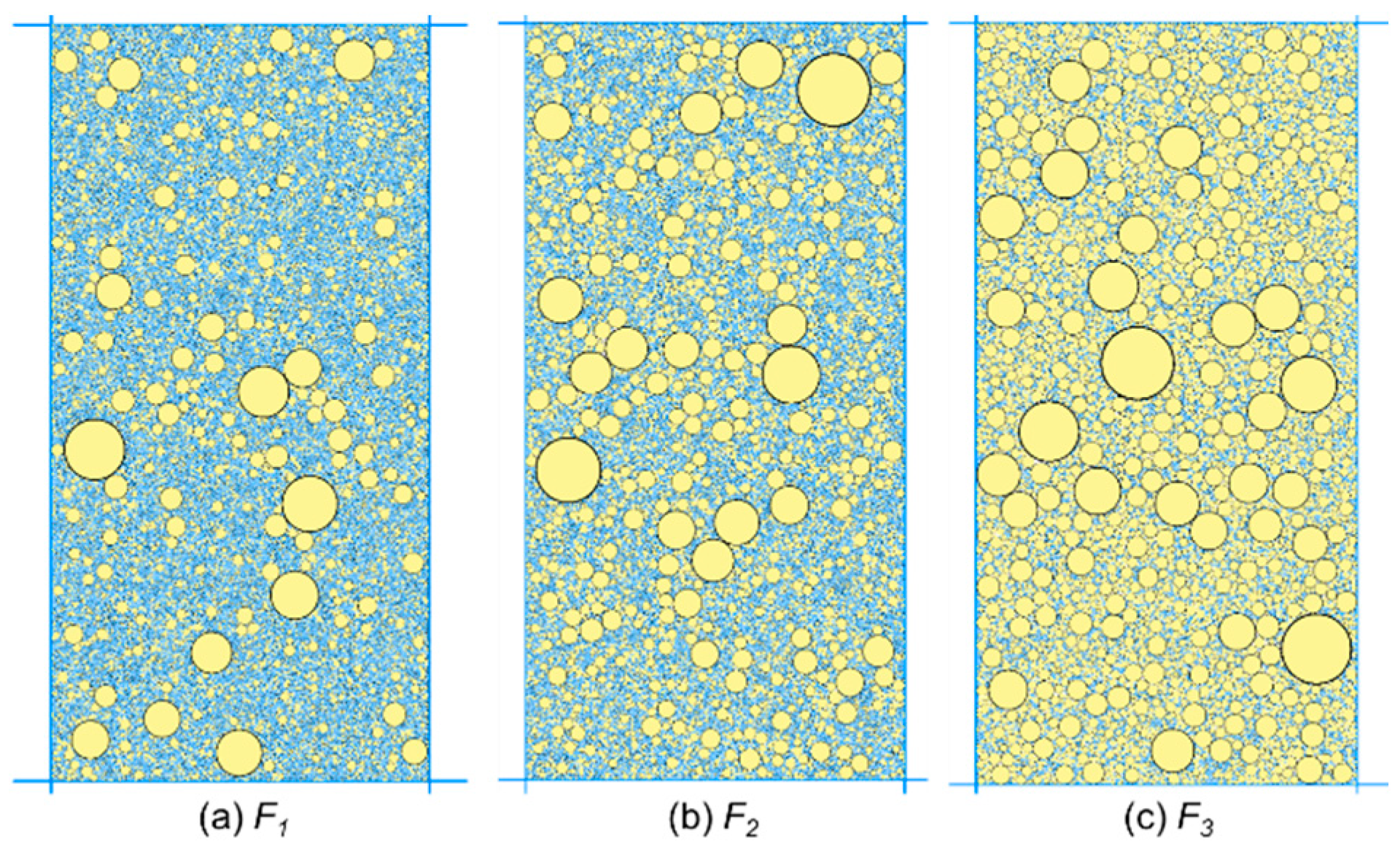
F1302.5182.6522.533
F2502.7712.6522.792
F3802.8642.6522.892
Table 3. The maximum deviatoric stress of the S–RM with different fractal dimensions and confining pressure.
Sample NumberAverage Fraction Dimension, DaveConfining Pressure
200 kPa300 kPa400 kPa600 kPa
F12.518962.491390.381483.372560.51
F22.771920.031249.751561.222254.78
F32.864946.921470.631726.822642.60
Disclaimer/Publisher’s Note: The statements, opinions and data contained in all publications are solely those of the individual author(s) and contributor(s) and not of MDPI and/or the editor(s). MDPI and/or the editor(s) disclaim responsibility for any injury to people or property resulting from any ideas, methods, instructions or products referred to in the content.

