Article

Complex Rayleigh–van-der-Pol–Duffing Oscillators: Dynamics, Phase, Antiphase Synchronization, and Image Encryption

by
Asma Al Themairi
1,*,
Gamal M. Mahmoud
2,
Ahmed A. Farghaly
2,3 and
Tarek M. Abed-Elhameed
2
1
Department of Mathematical Sciences, College of Science, Princess Nourah bint Abdulrahman University, P.O. Box 84428, Riyadh 11671, Saudi Arabia
2
Department of Mathematics, Faculty of Science, Assiut University, Assiut 71516, Egypt
3
Department of Information Technology, College of Computer and Information Sciences, Majmaah University, P.O. Box 66, Al-Majmaah 11952, Saudi Arabia
*
Author to whom correspondence should be addressed.
Fractal Fract. 2023, 7(12), 886; https://doi.org/10.3390/fractalfract7120886
Submission received: 6 November 2023 / Revised: 2 December 2023 / Accepted: 4 December 2023 / Published: 15 December 2023

Abstract

:
This paper introduces the complex Rayleigh–van-der- Pol–Duffing oscillators (RVDOs), which are hyperchaotic and can be autonomous or nonautonomous. The fundamental dynamics of the autonomous and nonautonomous complex RVDOs, including dissipation, symmetry, fixed points, and stability, are studied. These oscillators are found in various necessary fields of physics and engineering. The paper proposes a scheme to achieve phase synchronization (PS) and antiphase synchronization (APS) for different dimensional models. These kinds of synchronization are considered a generalization of several other types of synchronization. We use the active control method based on Lyapunov’s stability theory for this scheme. By analytically determining the control functions, the scheme achieved PS and APS. Our scheme is applied to study the PS of hyperchaotic behaviors for two distinct hyperchaotic nonautonomous and autonomous complex RVDOs. Additionally, the scheme is employed to achieve the APS of a chaotic real nonautonomous RVDO and a hyperchaotic complex autonomous RVDO, including those with different dimensions. Our work presents numerical results that plot the amplitudes and phases of these hyperchaotic behaviors, demonstrating the achievement of the PS and APS. The encryption and decryption of grayscale images are researched based on APS. The experimental results of image encryption and decryption are computed with information entropy, visual analysis, and histograms.

1. Introduction

The phase and antiphase synchronization of chaotic systems have gained significant interest because of their relevance to various fields and scenarios. These include lasers [1,2], complex networks [3], electrical circuits [4], memory processes [5], optical parametric oscillators [6], human cortex [7], fluids [8], neuroscience [9], ecological systems [10], coupled chemical oscillators [11], and the heartbeat and respiration cycle [12]. Many techniques to study the phase synchronization for the same dimension have been introduced, such as complete phase synchronization [13,14], antiphase synchronization [14], modified projective phase synchronization [15], and combination–combination phase synchronization [16]. On the other hand, different kinds of synchronization were introduced in the literature [17,18] and in the references therein. It is widely acknowledged that real-world models exhibit nonlinearity as a fundamental characteristic. Consequently, the dynamics of these models are mathematically depicted using nonlinear ODEs [19,20,21,22,23]. Kpomahou et al. [24] introduced the real Rayleigh–van-der-Pol–Duffing oscillator (RVDO) as:
u ¨ u + a u 3 e ( b c u 2 d u ˙ 2 ) u ˙ + e l ( 1 a u 2 ) u c o s ( 2 w t ) = e ( h + 2 m s i n ( Ω t ) ) c o s ( w t ) ,
where the expression u + a u 3 + e l ( 1 a u 2 ) u cos ( 2 w t ) represents the components of linear and nonlinear stiffness that contribute to the linear and nonlinear parametric excitation, e ( b + c u 2 + d u ˙ 2 ) u ˙ is the hybrid Rayleigh–van der Pol damping force, and e ( h + 2 m s i n ( Ω t ) ) c o s ( w t ) ) is the external excitation force, w and Ω represent the two frequencies of the force that are modulated in amplitude, while 2 m , h, and e stand for the degree of modulation, the unmodulated carrier amplitude, and a small quantity characterizing the smallness of the dissipative and forced terms, respectively. If one has v 1 = u , v 2 = u ˙ , the two first order ordinary differential equations of oscillator (1) are:
v ˙ 1 = v 2 , v ˙ 2 = v 1 a v 1 3 + e ( b c v 1 2 d v 2 2 ) v 2 e l ( 1 a v 1 2 ) v 1 c o s ( 2 w t ) + e ( h + 2 m s i n ( Ω t ) ) c o s ( w t ) .
If we consider that v 1 = z 1 + i z 2 and v 2 = z 3 + i z 4 , i = 1 are complex variables, then the 4D real form of the RVDO (2) is:
z ˙ 1 = z 3 , z ˙ 2 = z 4 , z ˙ 3 = z 1 a ( z 1 3 3 z 1 z 2 2 ) + e { b z 3 c [ ( z 1 2 z 2 2 ) z 3 2 z 1 z 2 z 4 ] d [ z 3 3 3 z 3 z 4 2 ] } e l { [ 1 a ( z 1 2 z 2 2 ) ] z 1 + 2 a z 1 z 2 2 } c o s ( 2 w t ) + e ( h + 2 m s i n ( Ω t ) ) c o s ( w t ) , z ˙ 4 = z 2 a ( z 2 3 + 3 z 1 2 z 2 ) e { b z 4 c [ ( z 1 2 z 2 2 ) z 4 + 2 z 1 z 2 z 3 ] d [ z 4 3 + 3 z 3 2 z 4 ] } e l { [ 1 a ( z 1 2 z 2 2 ) ] z 2 2 a z 1 2 z 2 } c o s ( 2 w t ) .
For the choice l = h = m = 0 , the autonomous form of RVDO (3) is given as:
z ˙ 1 = z 3 , z ˙ 2 = z 4 , z ˙ 3 = z 1 a ( z 1 3 3 z 1 z 2 2 ) + e { b z 3 c [ ( z 1 2 z 2 2 ) z 3 2 z 1 z 2 z 4 ] d [ z 3 3 3 z 3 z 4 2 ] } z ˙ 4 = z 2 a ( z 2 3 + 3 z 1 2 z 2 ) + e { b z 4 c [ ( z 1 2 z 2 2 ) z 4 + 2 z 1 z 2 z 3 ] d [ z 4 3 + 3 z 3 2 z 4 ] } .
This paper introduces hyperchaotic nonautonomous and autonomous complex Rayleigh–van-der-Pol–Duffing oscillators (3) and (4), respectively. We investigate the basic dynamics for these oscillators including dissipation, symmetry, fixed points, and their stability. Using the Lyapunov exponents [25], we prove that models (3) and (4) have hyperchaotic solutions. The paper proposes, also, a scheme utilizing an active control technique based on Lyapunov stability analysis to achieve phase synchronization (PS) and antiphase synchronization (APS) for different dimension models. According to the literature, these kinds of synchronization are a generalization of several other forms [14,15]. The encryption and decryption of the gray chemical plant image are examined using APS. For this image, we compute the visual analysis, information entropy, and histograms.
This paper is organized as follows: Section 2 contains the dynamics of the proposed complex oscillators (3) and (4), including fixed points and their stability, dissipation, symmetry, and chaotic behavior. In Section 3, we introduce a scheme to achieve PS and APS based on an active control technique and Lyapunov stability analysis. Section 4 and Section 5 deal with illustrative examples for the PS and APS, respectively. A gray image encryption application of APS is presented in Section 6. For the grayscale chemical plant image, the information entropy, visual analysis, and histograms are provided. Section 7 presents our conclusions.

2. Dynamics of Complex RVDOs (3) and (4)

This section presents the characteristics and behavior of our suggested autonomous RVDO (3) and nonautonomous RVDO (4). These models are dissipative under the condition e b < 0 . It is clear that model (3) is not symmetric and model (4) is symmetric under the transformation ( z 1 , z 2 , z 3 , z 4 ) ( z 1 , z 2 , z 3 , z 4 ) . Model RVDO (3) has no fixed points, while model (4) has three as: E 0 = ( 0 , 0 , 0 , 0 ) T and E 1 , 2 = ( ± 1 a , 0 , 0 , 0 ) T for a > 0 . To study the stability of E 0 = ( 0 , 0 , 0 , 0 ) T , we calculate the Jacobian matrix of the model (4) at E 0 as:
0 0 1 0 0 0 0 1 1 0 e b 0 0 1 0 e b ,
and its eigenvalues are: μ 1 , 2 = μ 3 , 4 = b e ± b 2 e 2 + 4 2 . It is clear that E 0 is not stable for any values of the parameters e and b. The fixed points E 1 , 2 can be similarly studied to E 0 .
We chose a = 1.25 , b = 0.5 , c = 0.085 , e = 1 , h = 1 , m = 0.5 , l = 0.05 , w = 1 , and Ω = 1 and calculated the Lyapunov exponents [25] for the real autonomous RVDO (2), the complex autonomous RVDO (3) and the complex nonautonomous RVDO (4). We found those values are ( λ 1 = 0.1556 ,   λ 2 = 0 ,   λ 3 = 0.4198 ) , ( λ 1 , 2 = 0.028 , λ 3 = 0 , λ 4 = 0.7289 ,   λ 5 = 0.6709 ) , and ( λ 1 , 2 = 0.0878 ,   λ 3 = 0.3291 ,   λ 4 = 5.1644 ) , respectively. This means that the real autonomous RVDO (2) has a chaotic solution, the complex autonomous RVDO (3) has a hyperchaotic solution of order 2, and the complex nonautonomous RVDO (4) has a hyperchaotic solution of order 2 as shown in Figure 1, Figure 2 and Figure 3.
In the following remarks, we present the differences between models (2)–(4).
Remark 1.
Model (3) is considered a generalization of model (2).
Remark 2.
Model (3) is not symmetric, and model (4) is symmetric.
Remark 3.
Model (4) has three fixed points, while model (3) does not.
Remark 4.
It is observed that the count of Lyapunov exponents in nonautonomous models is higher by one compared to autonomous models with the same dimensions. This difference arises due to the inclusion of time as an additional dimension in the nonautonomous models.

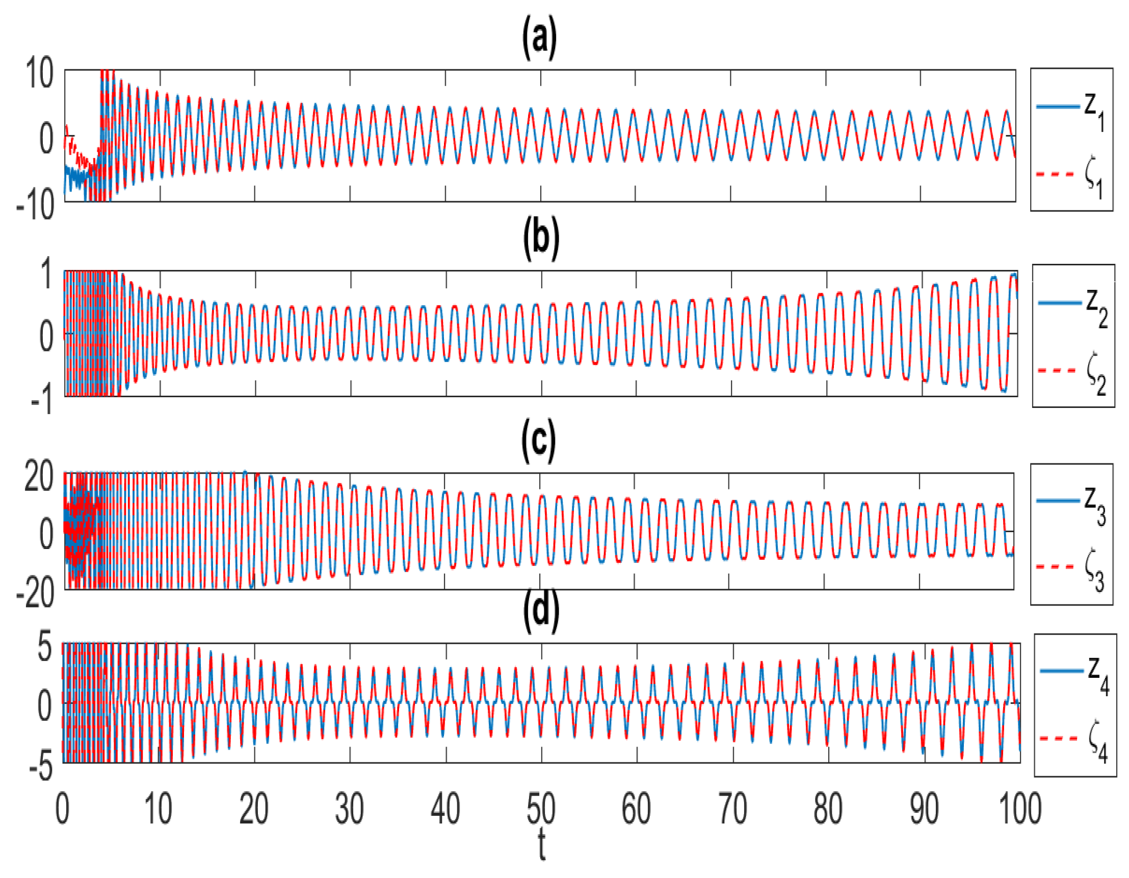
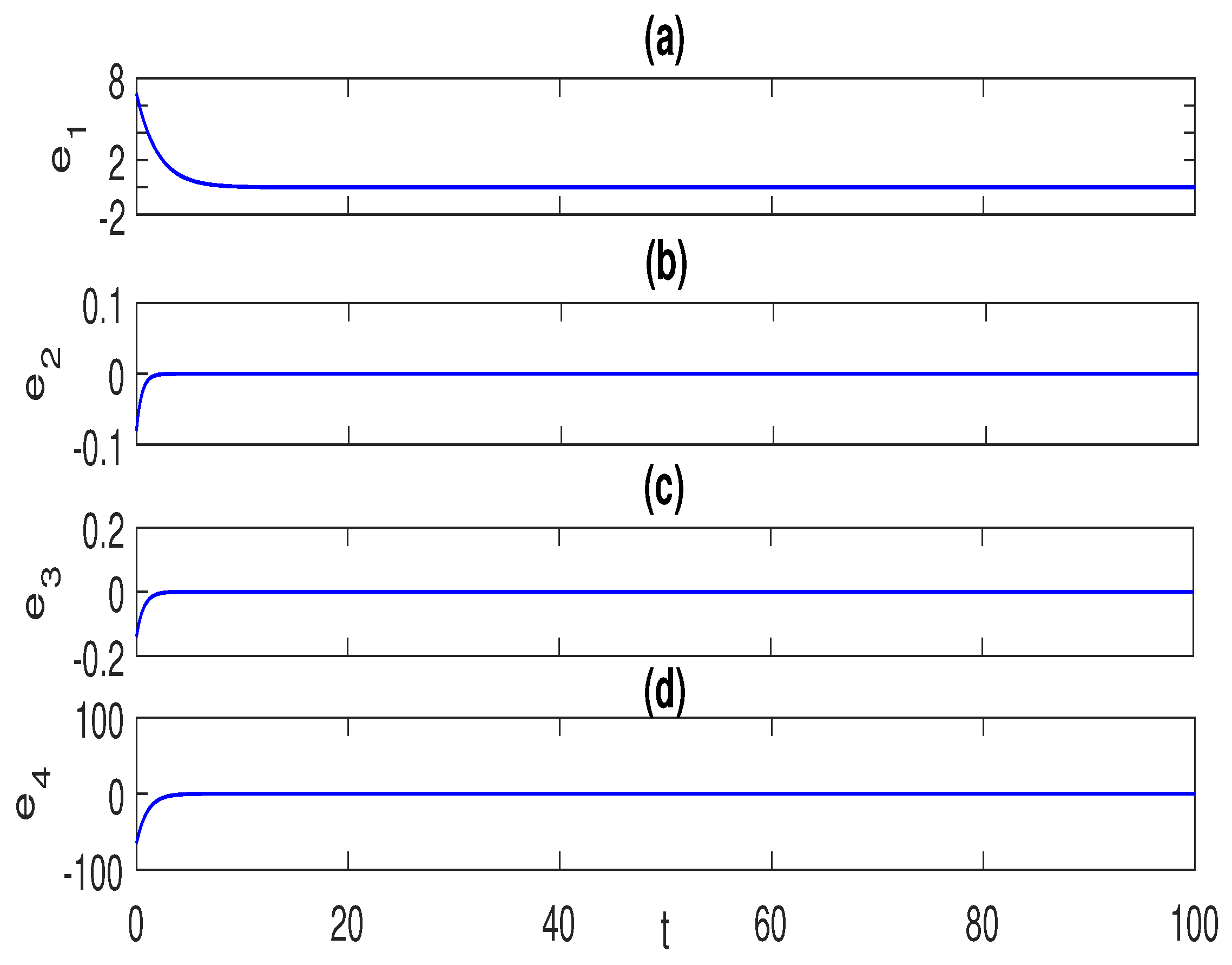
3. A Scheme for PS and APS with Different Dimensions

Our plan assumes a single master model and a single slave system. The master system represents:
z ˙ = f ( z , t ) ,
while the slave model is:
ζ ˙ = g ( ζ , t ) + u ,
where z R n , ζ R m are the state vectors of models, and u R m is the control function which will be calculated.
Definition 1.
PS can be observed in the master system (6) as well as the slave system (7), provided that there exist two constant matrices A R n × n and B R n × m in the real matrix space, if
lim x E = lim x B ζ A z = C ,
where  E = ( e 1 , e 2 , , e n ) T R n  is the error vector, and C is a constant vector.
Remark 5.
The APS for different dimensions can be obtained if one takes A = A in Equation (8).
Remark 6.
If ζ i n R n and A = B = I R n × n , then the PS for different dimensions is converted to the PS with the same dimensions [14].
Remark 7.
The modified PS with the same dimensions can be obtained from Equation (8), if one chooses ζ i n R n and B R n × n [15].
Theorem 1.
We can achieve PS among two distinct models (6) and (7), if we design the vector of the control functions U R n in the following way:
U B u = A f ( z , t ) B g ( ζ , t ) K E ,
where K = d i a g ( k 1 , k 2 , , k n ) is the control gain diagonal matrix.
Proof. 
From Equation (8), we have
E = B ζ A z ,
by taking the derivative of Equation (10) with respect to time, we derive the following expression:
E ˙ = B ζ ˙ A z ˙ ,
using Equations (6), (7) and (9), we obtain
E ˙ = K E ,
and by utilizing Lyapunov stability analysis, if we assign K to be zero, Equation (12) can be expressed in the following form E ˙ = 0 . This means that E C as t ; then, PS is achieved. □
Corollary 1.
For the choice k i < 0 and using the stability theory, E 0 as t .
Corollary 2.
According to Remark 5, the APS between the models (6) and (7) can be achieved if the control functions take the form:
U B u = A f ( z , t ) B g ( ζ , t ) K E .
The phase differences Δ i j between the k = 1 n A i k z k , k = 1 n A j k z k projection for the master model and the l = 1 m B i l ζ l , l = 1 m B j l ζ l projection for the slave one are described as follows:
Δ i j = ψ i j d ψ i j r ,
where i , j = 1 , 2 , 3 , , n , i j , ψ i j d = t a n 1 k = 1 n A j k z k k = 1 n A i k z k and ψ i j r = t a n 1 l = 1 m B j l ζ l l = 1 m B i l ζ l . The occurrence of the PS is dependent on the bounded nature of these phase differences.
The definitions of the amplitudes in the k = 1 n A i k z k , k = 1 n A j k z k projection for the master model and the l = 1 m B i l ζ l , l = 1 m B j l ζ l projection for the slave one are as follows:
A i j d = k = 1 n A i k z k 2 + k = 1 n A j k z k 2 , A i j r = l = 1 m B i l ζ l 2 + l = 1 m B j l ζ l 2 .
Subsequently, we utilize this approach to examine the occurrence of PS in Section 4 and APS in Section 5 by applying it to hyperchaotic attractors (2)–(4).

4. Illustrative Example for PS

In this section, we test the PS technique using an example. We consider the model (3) as the master model, and the slave one is model (4). The slave model can be written after adding the control functions as:
ζ ˙ 1 = ζ 3 + u 1 , ζ ˙ 2 = ζ 4 + u 2 , ζ ˙ 3 = ζ 1 a ( ζ 1 3 3 ζ 1 ζ 2 2 ) + e { b ζ 3 c [ ( ζ 1 2 ζ 2 2 ) ζ 3 2 ζ 1 ζ 2 ζ 4 ] d [ ζ 3 3 3 ζ 3 ζ 4 2 ] } + u 3 , ζ ˙ 4 = ζ 2 a ( ζ 2 3 + 3 ζ 1 2 ζ 2 ) e { b ζ 4 c [ ( ζ 1 2 ζ 2 2 ) ζ 4 + 2 ζ 1 ζ 2 ζ 3 ] d [ ζ 4 3 + 3 ζ 3 2 ζ 4 ] } + u 4 ,
where u = ( u 1 , u 2 , u 3 , u 4 ) T is the control functions.
For the choice A = B = I 4 × 4 and applying Theorem 1, the control functions (9) can be written as:
U 1 u 1 = z 3 ζ 3 k 1 e 1 , U 2 u 2 = z 4 ζ 4 k 2 e 2 , U 3 u 3 = z 1 a ( z 1 3 3 z 1 z 2 2 ) + e { b z 3 c [ ( z 1 2 z 2 2 ) z 3 2 z 1 z 2 z 4 ] d [ z 3 3 3 z 3 z 4 2 ] } e l { [ 1 a ( z 1 2 z 2 2 ) ] z 1 + 2 a z 1 z 2 2 } c o s ( 2 w t ) + e ( h + 2 m s i n ( Ω t ) ) c o s ( w t ) ζ 1 + a ( ζ 1 3 3 ζ 1 ζ 2 2 ) e { b ζ 3 c [ ( ζ 1 2 ζ 2 2 ) ζ 3 2 ζ 1 ζ 2 ζ 4 ] d [ ζ 3 3 3 ζ 3 ζ 4 2 ] } k 3 e 3 , U 4 u 4 = z 2 a ( z 2 3 + 3 z 1 2 z 2 ) e { b z 4 c [ ( z 1 2 z 2 2 ) z 4 + 2 z 1 z 2 z 3 ] d [ z 4 3 + 3 z 3 2 z 4 ] } e l { [ 1 a ( z 1 2 z 2 2 ) ] z 2 2 a z 1 2 z 2 } c o s ( 2 w t ) ζ 2 + a ( ζ 2 3 + 3 ζ 1 2 ζ 2 ) e { b ζ 4 c [ ( ζ 1 2 ζ 2 2 ) ζ 4 + 2 ζ 1 ζ 2 ζ 3 ] d [ ζ 4 3 + 3 ζ 3 2 ζ 4 ] } k 4 e 4 .
During the numerical simulation, we use the same parameters and initial conditions of the master and slave models (3) and (16) of Figure 2 and Figure 3. For the choice K = 0 , the results of PS are shown in Figure 4, Figure 5 and Figure 6. Figure 4 and Figure 5 show the phase differences for six plane projections vs. t. The confirmation of achieving PS is supported by the observation that the phase differences remain within a bounded range. The amplitudes of the master and the slave models in ( z 1 , z 3 ) and ( ζ 1 , ζ 3 ) spaces ( A 13 d and A 13 r ) are shown in Figure 6a,b, and Figure 6c displays A 13 d vs. A 13 r . Figure 6 demonstrates that these amplitudes exhibit hyperchaotic behavior and are uncorrelated. Similar results are observed for the other amplitudes of the master and slave systems in different plane projections.
For K = d i a g ( 0.5 , 2 , 1.5 , 1 ) , the state variables for the master model (3) and the slave model (16) are shown in Figure 7. Figure 8 depicts the synchronization errors, which approach zero.

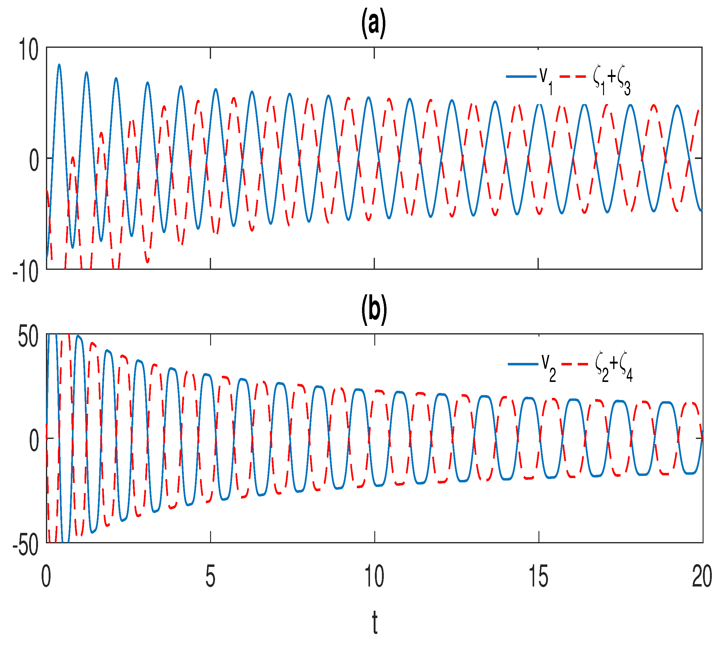
5. Illustrative Example for APS

In this section, we introduce an example for APS with different dimensions. We consider the model (2) as the 2D master model, and model (16) is the 4D slave one.
For the choice A = I 2 × 2 and B = 1 0 1 0 0 1 0 1 and applying Corollary 2, the control functions (13) can be written as:
U 1 u 1 + u 3 = v 2 ζ 3 ( ζ 1 a ( ζ 1 3 3 ζ 1 ζ 2 2 ) + e { b ζ 3 c [ ( ζ 1 2 ζ 2 2 ) ζ 3 2 ζ 1 ζ 2 ζ 4 ] d [ ζ 3 3 3 ζ 3 ζ 4 2 ] } + u 3 ) k 1 e 1 , U 2 u 2 + u 4 = ( v 1 a v 1 3 + e ( b c v 1 2 d v 2 2 ) v 2 e l ( 1 a v 1 2 ) v 1 c o s ( 2 w t ) + e ( h + 2 m s i n ( Ω t ) ) c o s ( w t ) ) ζ 4 ( ζ 2 a ( ζ 2 3 + 3 ζ 1 2 ζ 2 ) e { b ζ 4 c [ ( ζ 1 2 ζ 2 2 ) ζ 4 + 2 ζ 1 ζ 2 ζ 3 ] d [ ζ 4 3 + 3 ζ 3 2 ζ 4 ] } ) k 2 e 2 .
In the numerical simulation, we use the same parameters and initial conditions of the master and slave models (2) and (16) of Figure 1 and Figure 3. For the choice K = 0 , the results of the PS are shown in Figure 9 and Figure 10. Figure 9 depicts the phase differences for one plane projection vs. t. The fact that the phase differences are bounded confirms the achievement of PS. The amplitudes of the master and the slave models in ( v 1 , v 2 ) and ( ζ 1 + ζ 3 , ζ 2 + ζ 4 ) spaces ( A 12 d and A 12 r ) are shown in Figure 10a,b, and Figure 6c displays A 12 d vs. A 12 r . Figure 10 demonstrates that these amplitudes exhibit hyperchaotic behavior and are uncorrelated (linearly independent).
For K = d i a g ( 0.5 , 2 ) , the state variables for the master model (2) and the slave model (16) are shown in Figure 11. Figure 12 depicts the synchronization errors, which approach zero.

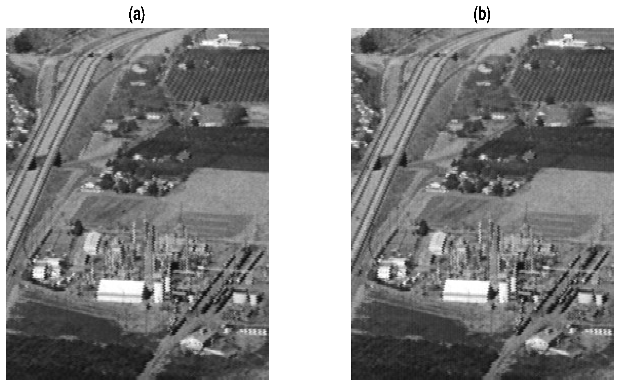
6. An Image Encryption for APS

The use of image encryption based on the APS between chaotic RVDOs (2) and (16) is examined in this part. The slave model (16) is driven by signals from the master model (2), which we take to be the master model in the sender. These signals produce a sequence of chaotic signals, which in turn drive the master model (2) at synchronization.

6.1. The Process of Encryption

In the encryption process, the following major steps are outlined. Firstly, an M × N grayscale image is represented as a matrix of pixels as:
G = G 11 G 12 G 1 N G M 1 G M 2 G M N .
This matrix is then converted into a 1D vector, where each element represents a gray value ranging from 0 to 255 as follows:
P = [ G 11 , G 12 , , G 1 N , G 21 , G 22 , , G 2 N , G M 1 , G M 2 , , G M N ] = [ L 1 , L 2 , , L M N ] .
Next, a chaotic decimal sequence is generated based on the APS of the master model (2) and the slave model (16), discarding the initial values to obtain a sequence of length MN as:
C S = [ C S 1 , C S 2 , , C S M N ] .
This chaotic sequence is sorted in ascending order, and integer values K are calculated using a formula involving the rounded floor of the chaotic sequence as follows:
K = m o d ( f l o o r ( C S ) × 10 15 , 256 ) .
Then, an exclusive XOR operation is performed between the integer values K and the vector P to create the encrypted vector HG.
H G = K P ,
where ⊕ is the exclusive X O R operation.
Finally, the encrypted vector is converted back into a 2D matrix to produce the ciphered image of size M × N.

6.2. The Process of Decryption

The encryption procedure is both symmetric and reversible. As most people know, decryption is the opposite of encryption, and the keys required for both processes are the same.

6.3. Experimental Results

The efficiency of encrypting and decrypting grayscale images is evaluated in this subsection. Various techniques, including information entropy, histogram, and visual analysis, are used to assess the application’s performance. The 256 × 256 test image, chemical plant, is shown in Figure 13a and was used for this evaluation.

6.3.1. Visual Analysis

This subsection assesses how closely and differently the original and decrypted images resemble each other using visual analysis. The simulation results are shown in Figure 13, where Figure 13a shows the original image (chemical plant), and Figure 13b depicts the decrypted image. The decrypted image is the same as the original, whereas the encrypted image has noise. This shows that our image encryption approach successfully encrypts and decrypts grayscale images.

6.3.2. Information Entropy

A measure of an image’s randomness is called information entropy, and it is computed as follows:
H ( I ) = k = 1 M q ( k ) log 2 1 q ( k ) .
In image I, q ( k ) indicates the probability of an intensity value k, and M represents the maximum feasible intensity value.
The encryption approach produced chemical plant images with information entropy values of 7.3399 and 7.3424 for the original and decrypted images, respectively. With an information entropy of nearly 8, the suggested method is very close to the optimal value and contains considerable randomness. This indicates that the proposed method has a minimal possibility of leaking information.

6.3.3. Histogram Analysis

The total number of pixels with intensity i is given by the histogram h ( i ) for an image with intensity values between 0 and L. The frequency of the encrypted and decrypted images can be examined using this histogram. It is imperative to remember that the histogram of an encrypted image must differ from the image’s before encryption. The original chemical plant and decrypted image histograms are displayed in Figure 14, respectively.
A grayscale image’s histogram is not evenly distributed. By dividing the pixels in the encrypted image equally, the suggested encryption algorithm can conceal statistical information from the plain image.

7. Conclusions

In conclusion, this paper has introduced the hyperchaotic nonautonomous and autonomous complex Rayleigh–van-der-Pol–Duffing oscillators (RVDOs) (3) and (4). We studied the fundamental dynamics of these oscillators, such as stability, fixed points, and dissipation. We demonstrated the hyperchaotic solutions of models (3) and (4) using the Lyapunov exponents, as shown in Figure 1, Figure 2 and Figure 3. The hyperchaotic nature of these models may be used in numerous significant engineering and scientific domains. The proposed scheme in Section 3, utilizing an active control technique based on Lyapunov stability analysis, aims to achieve PS and APS for different dimensional models. The scheme successfully achieved PS and APS through the analytical determination of control functions (9) and (13). These types of synchronization are considered a generalization of many types in the literature [14,15]. The scheme is applied to investigate the PS of hyperchaotic attractors (3) and (4). To achieve APS, we used the models (2) and (4), including those with different dimensions. The presented numerical results illustrate the phases and amplitudes of these chaotic and hyperchaotic attractors and provide evidence of the effective accomplishment of PS and APS. These results are shown in Figure 4, Figure 5, Figure 6, Figure 7, Figure 8, Figure 9, Figure 10, Figure 11 and Figure 12. Using the APS, a grayscale image encryption technique is offered. Figure 13 displays the simulation results for the original and decrypted images. The information entropy of both the plain and decrypted images was computed and analyzed. They were closer to the optimal value of 8. As demonstrated in Figure 14, the encrypted image distributions are uniform, but the ciphered picture histograms are nearly flat. The encryption and decryption results for the gray chemical plant images were displayed using the Matlab application.
Shortly, we hope to expand these studies to include phase combination synchronization and phase combination–combination synchronization with various dimensions.

Author Contributions

Conceptualization, G.M.M.; Software, T.M.A.-E.; Validation, A.A.T.; Formal analysis, A.A.F. All authors have read and agreed to the published version of the manuscript.

Funding

Funding for this manuscript was provided by Princess Nourah bint Abdulrahman University Researchers Supporting Project number (PNURSP2023R295).

Data Availability Statement

No data were used to support this study.

Acknowledgments

Princess Nourah bint Abdulrahman University Researchers Supporting Project number (PNURSP2023R295) Princess Nourah bint Abdulrahman University, Riyadh, Saudi Arabia.

Conflicts of Interest

The authors declare no conflict of interest.

References

  1. Hillbrand, J.; Auth, D.; Piccardo, M.; Opačak, N.; Gornik, E.; Strasser, G.; Capasso, F.; Breuer, S.; Schwarz, B. In-phase and anti-phase synchronization in a laser frequency comb. Phys. Rev. Lett. 2020, 124, 023901. [Google Scholar] [CrossRef]
  2. Mao, X.; Sun, Y.; Wang, L.; Guo, Y.; Gao, Z.; Wang, Y.; Li, S.; Yan, L.; Wang, A. Instability of optical phase synchronization between chaotic semiconductor lasers. Opt. Lett. 2021, 46, 2824–2827. [Google Scholar] [CrossRef]
  3. Dörfler, F.; Bullo, F. Synchronization in complex networks of phase oscillators: A survey. Automatica 2014, 50, 1539–1564. [Google Scholar] [CrossRef]
  4. Xie, Y.; Yao, Z.; Ma, J. Phase synchronization and energy balance between neurons. Front. Inf. Technol. Electron. Eng. 2022, 23, 1407–1420. [Google Scholar] [CrossRef]
  5. Fell, J.; Axmacher, N. The role of phase synchronization in memory processes. Nat. Rev. Neurosci. 2011, 12, 105–118. [Google Scholar] [CrossRef]
  6. Xiu-Qin, F.; Ke, S. Phase synchronization and anti-phase synchronization of chaos for degenerate optical parametric oscillator. Chin. Phys. 2005, 14, 1526. [Google Scholar] [CrossRef]
  7. Arnulfo, G.; Wang, S.H.; Myrov, V.; Toselli, B.; Hirvonen, J.; Fato, M.; Nobili, L.; Cardinale, F.; Rubino, A.; Zhigalov, A.; et al. Long-range phase synchronization of high-frequency oscillations in human cortex. Nat. Commun. 2020, 11, 5363. [Google Scholar] [CrossRef]
  8. Chakrabarti, B.; Shelley, M.J.; Fürthauer, S. Collective Motion and Pattern Formation in Phase-Synchronizing Active Fluids. Phys. Rev. Lett. 2023, 130, 128202. [Google Scholar] [CrossRef]
  9. Tallon-Baudry, C.; Bertrand, O.; Delpuech, C.; Pernier, J. Stimulus specificity of phase-locked and non-phase-locked 40 Hz visual responses in human. J. Neurosci. 1996, 16, 4240–4249. [Google Scholar] [CrossRef]
  10. Blasius, B.; Huppert, A.; Stone, L. Complex dynamics and phase synchronization in spatially extended ecological systems. Nature 1999, 399, 354–359. [Google Scholar] [CrossRef]
  11. Totz, J.F.; Snari, R.; Yengi, D.; Tinsley, M.R.; Engel, H.; Showalter, K. Phase-lag synchronization in networks of coupled chemical oscillators. Phys. Rev. E 2015, 92, 022819. [Google Scholar] [CrossRef]
  12. Kurths, J.; Schäfer, C.; Rosenblum, M.; Abel, H.H. Synchronization in Human Cardiorespiratory System. In Proceedings of the APS March Meeting Abstracts, Los Angeles, CA, USA, 16–20 March 1998; p. Q12.05. [Google Scholar]
  13. Shi, Y.; Li, T.; Zhu, J. Complete Phase Synchronization of Nonidentical High-Dimensional Kuramoto Model. J. Stat. Phys. 2023, 190, 6. [Google Scholar] [CrossRef]
  14. Mahmoud, G.M.; Mahmoud, E.E. Phase and antiphase synchronization of two identical hyperchaotic complex nonlinear systems. Nonlinear Dyn. 2010, 61, 141–152. [Google Scholar] [CrossRef]
  15. Mahmoud, E.E. Modified projective phase synchronization of chaotic complex nonlinear systems. Math. Comput. Simul. 2013, 89, 69–85. [Google Scholar] [CrossRef]
  16. Yadav, V.K.; Prasad, G.; Srivastava, M.; Das, S. Combination–combination phase synchronization among non-identical fractional order complex chaotic systems via nonlinear control. Int. J. Dyn. Control 2019, 7, 330–340. [Google Scholar] [CrossRef]
  17. Mahmoud, G.M.; Ahmed, M.E.; Abed-Elhameed, T.M. On fractional-order hyperchaotic complex systems and their generalized function projective combination synchronization. Optik 2017, 130, 398–406. [Google Scholar] [CrossRef]
  18. Boccaletti, S.; Kurths, J.; Osipov, G.; Valladares, D.; Zhou, C. The synchronization of chaotic systems. Phys. Rep. 2002, 366, 1–101. [Google Scholar] [CrossRef]
  19. Kpomahou, Y.; Adéchinan, J.; Hinvi, L. Effects of quartic nonlinearities and constant excitation force on nonlinear dynamics of plasma oscillations modeled by a Liénard-type oscillator with asymmetric double well potential. Indian J. Phys. 2022, 96, 3247–3266. [Google Scholar] [CrossRef]
  20. Mahmoud, G.M.; Abed-Elhameed, T.M.; Elbadry, M.M. A class of different fractional-order chaotic (hyperchaotic) complex duffing-van der pol models and their circuits implementations. J. Comput. Nonlinear Dyn. 2021, 16, 121005. [Google Scholar] [CrossRef]
  21. Mahmoud, G.M.; Abed-Elhameed, T.M.; Khalaf, H. On fractional and distributed order hyperchaotic systems with line and parabola of equilibrium points and their synchronization. Phys. Scr. 2021, 96, 115201. [Google Scholar] [CrossRef]
  22. Zhu, Q.; Wang, H. Output feedback stabilization of stochastic feedforward systems with unknown control coefficients and unknown output function. Automatica 2018, 87, 166–175. [Google Scholar] [CrossRef]
  23. Li, W.; Guan, Y.; Cao, J.; Xu, F. A note on global stability of a degenerate diffusion avian influenza model with seasonality and spatial Heterogeneity. Appl. Math. Lett. 2024, 148, 108884. [Google Scholar] [CrossRef]
  24. Kpomahou, Y.; Agbélélé, K.; Tokpohozin, N.; Yamadjako, A. Influence of Amplitude-Modulated Force and Nonlinear Dissipation on Chaotic Motions in a Parametrically Excited Hybrid Rayleigh–Van der Pol–Duffing Oscillator. Int. J. Bifurc. Chaos 2023, 33, 2330006. [Google Scholar] [CrossRef]
  25. Wolf, A.; Swift, J.B.; Swinney, H.L.; Vastano, J.A. Determining Lyapunov exponents from a time series. Phys. D Nonlinear Phenom. 1985, 16, 285–317. [Google Scholar] [CrossRef]
Figure 1. Chaotic solution of model RVDO (2) for d = 0 and the initial values v 0 = ( 0.1 , 0.1 ) T in ( v 1 , v 2 ) space.
Fractalfract 07 00886 g001
Figure 2. Hyperchaotic solution of model RVDO (3) for d = 0.2 and the initial values z 0 = ( 0.1 , 0.1 , 0.1 , 0.1 ) T in ( z 1 , z 3 ) space.
Fractalfract 07 00886 g002
Figure 3. Hyperchaotic solution of model RVDO (4) for d = 0 and the initial values z 0 = ( 0.1 , 0.1 , 0.1 , 0.1 ) T in ( z 3 , z 4 ) space.
Fractalfract 07 00886 g003
Figure 4. The phase differences of the PS between the master model (3) and slave model (16) for different plane projections vs. t: (a) Δ 12 , (b) Δ 13 , (c) Δ 14 .
Fractalfract 07 00886 g004
Figure 5. The phase differences of the PS between the master model (3) and slave model (16) for different plane projections vs. t: (a) Δ 24 , (b) Δ 23 , (c) Δ 34 .
Fractalfract 07 00886 g005
Figure 6. The amplitudes of the master and the slave models in ( z 1 , z 3 ) and ( ζ 1 , ζ 3 ) spaces: (a) A 13 d vs. t, (b) A 13 r vs. t, (c) ( A 13 d , A 13 r ) space.
Fractalfract 07 00886 g006
Figure 7. The state variables for the master model (3) and the slave model (16) after PS: (a) z 1 and ζ 1 vs. t, (b) z 2 and ζ 2 vs. t, (c) z 3 and ζ 3 vs. t, (d) z 4 and ζ 4 vs. t.
Fractalfract 07 00886 g007
Figure 8. The synchronization errors of the master model (3) and the slave model (16): (a) e 1 vs. t, (b) e 2 vs. t, (c) e 3 vs. t, (d) e 4 vs. t.
Fractalfract 07 00886 g008
Figure 9. The phase differences of APS between the master model (2) and slave model (16) for the projection ( v 1 , v 2 ) vs. t.
Fractalfract 07 00886 g009
Figure 10. The amplitudes of the master model (2) and the slave model (16) in ( v 1 , v 2 ) and ( ζ 1 + ζ 3 , ζ 2 + ζ 4 ) spaces: (a) A 12 d vs. t, (b) A 1324 r vs. t, (c) ( A 12 d , A 1324 r ) space.
Fractalfract 07 00886 g010
Figure 11. The state variables for the master model (2) and the slave model (16) after APS: (a) v 1 and ζ 1 + ζ 3 vs. t, (b) v 2 and ζ 2 + ζ 4 vs. t.
Fractalfract 07 00886 g011
Figure 12. The synchronization errors of the master model (2) and the slave model (16): (a) e 1 vs. t, (b) e 2 vs. t.
Fractalfract 07 00886 g012
Figure 13. Chemical plant images: (a) original, and (b) decrypted.
Fractalfract 07 00886 g013
Figure 14. Analysis of the histogram of the chemical plant: (a) original image, and (b) decrypted image.
Fractalfract 07 00886 g014
Disclaimer/Publisher’s Note: The statements, opinions and data contained in all publications are solely those of the individual author(s) and contributor(s) and not of MDPI and/or the editor(s). MDPI and/or the editor(s) disclaim responsibility for any injury to people or property resulting from any ideas, methods, instructions or products referred to in the content.

