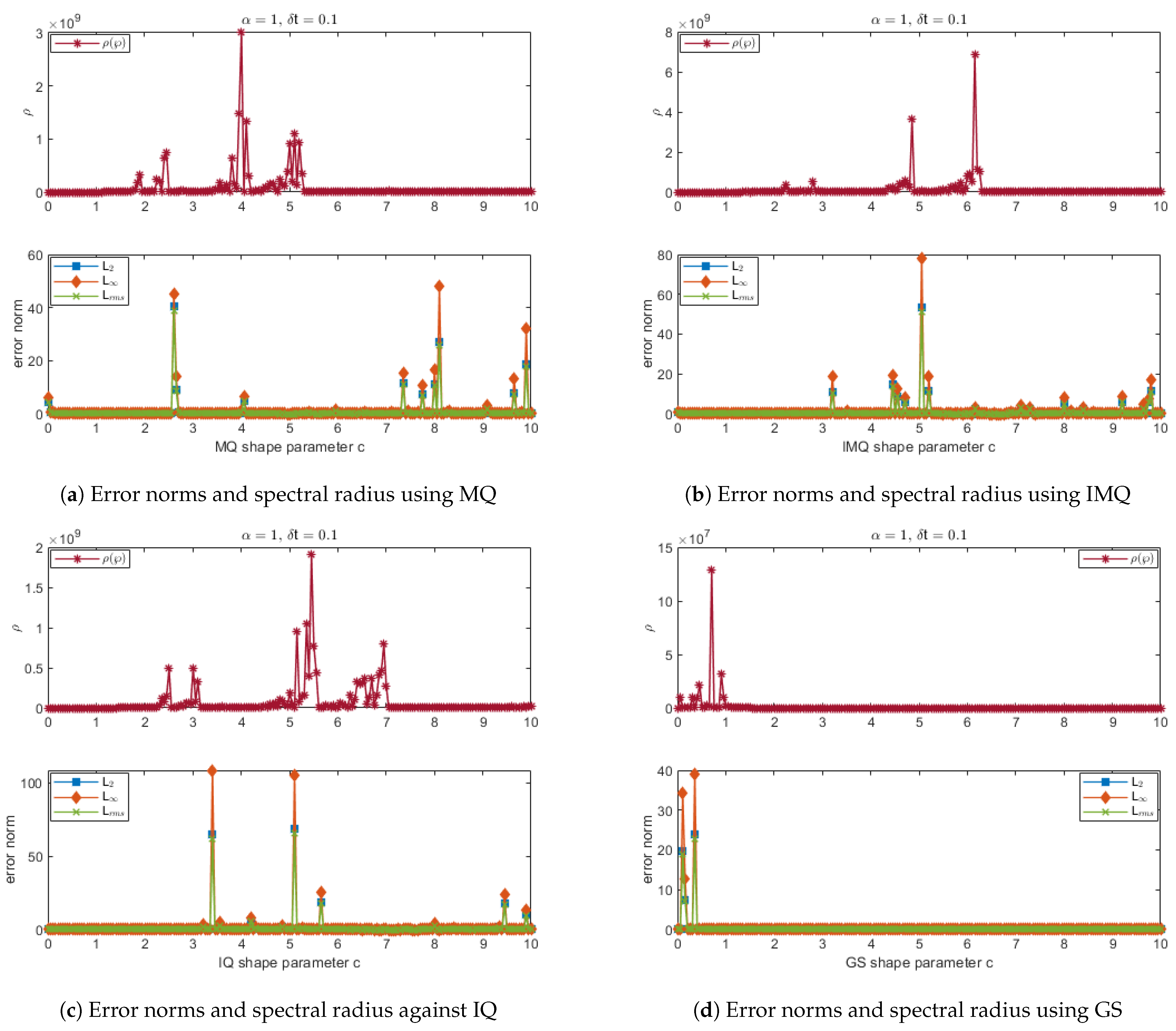
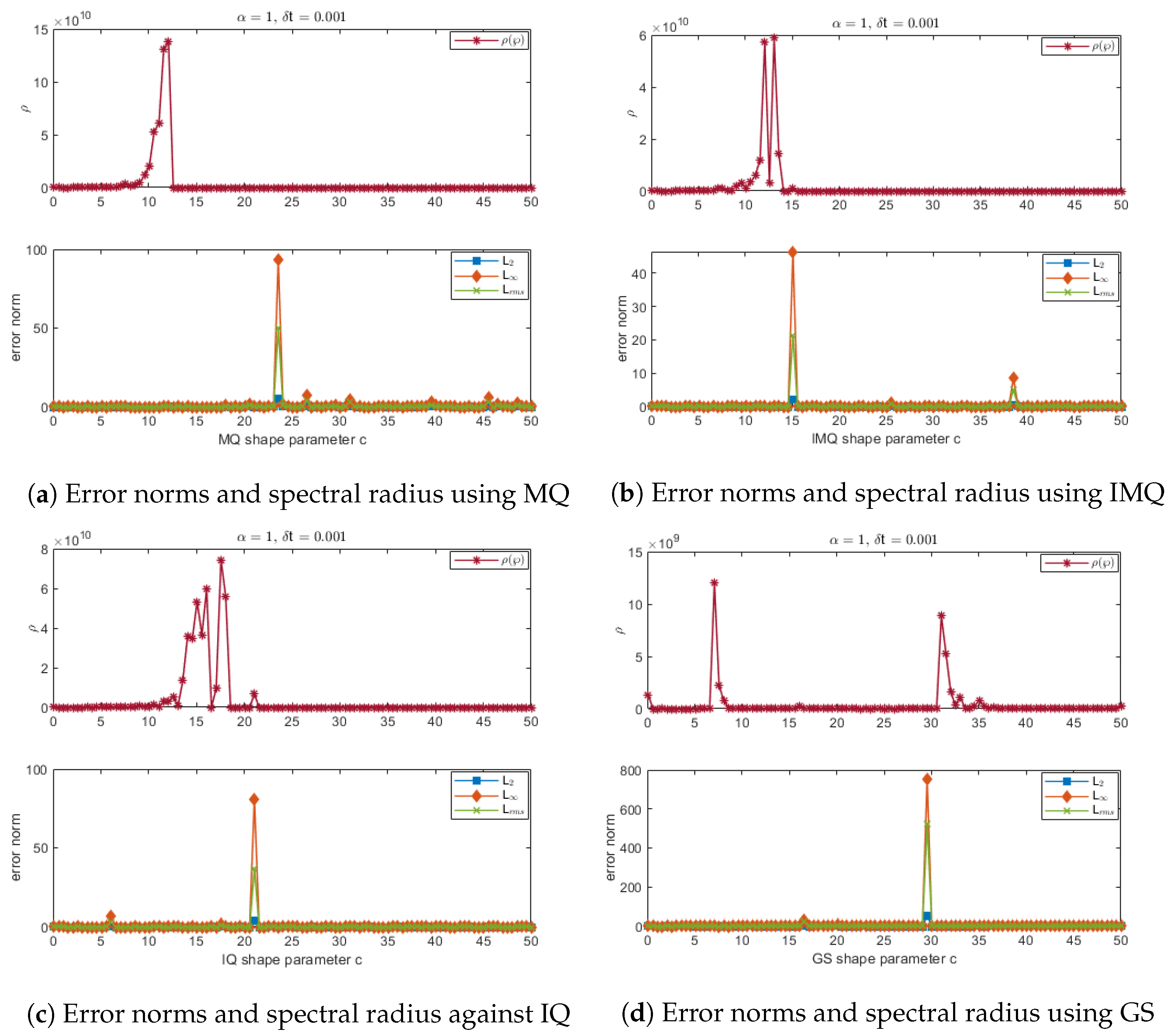
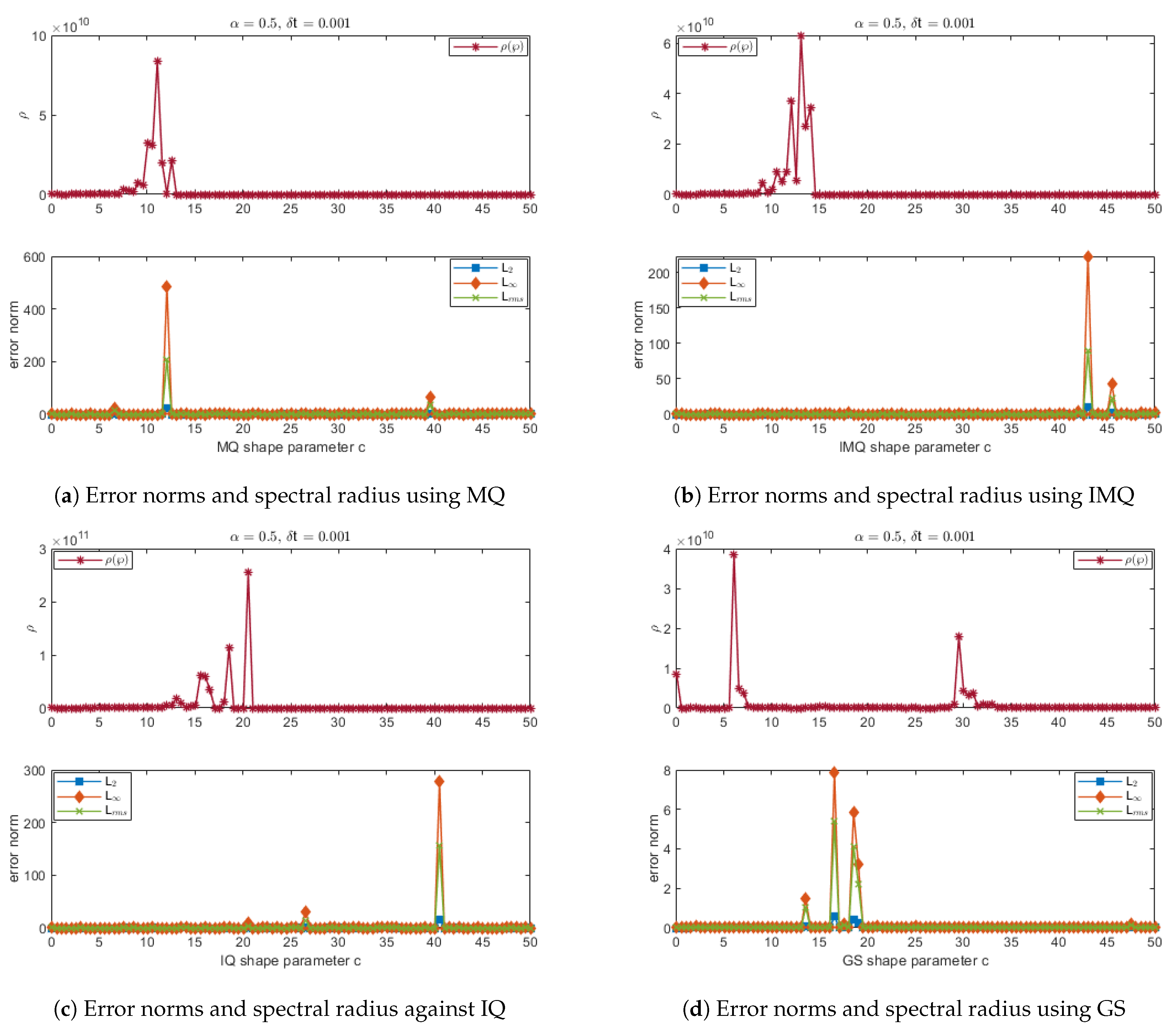
Figure 1.
Error norms and spectral radius correspond to Example 1 when , using MQ, IMQ, IQ, and GS RBFs.
Figure 1.
Error norms and spectral radius correspond to Example 1 when , using MQ, IMQ, IQ, and GS RBFs.
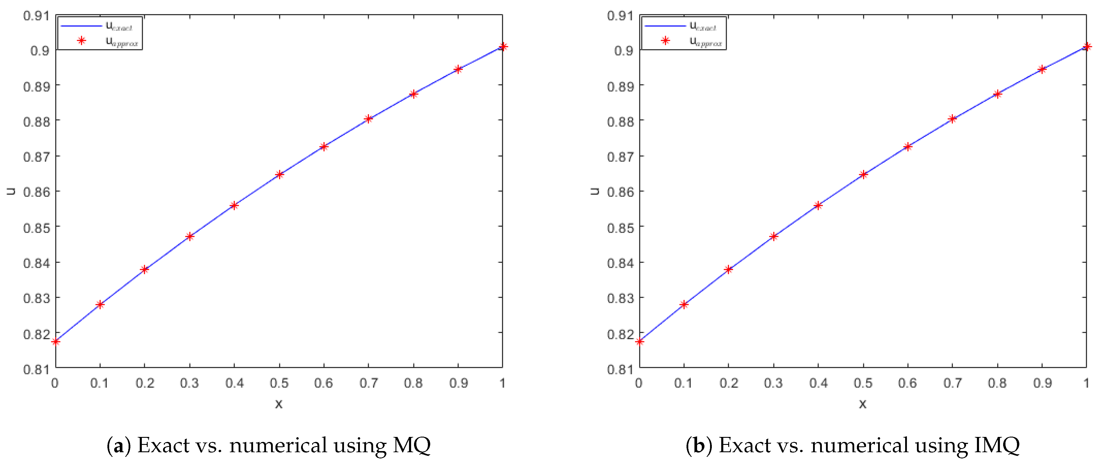
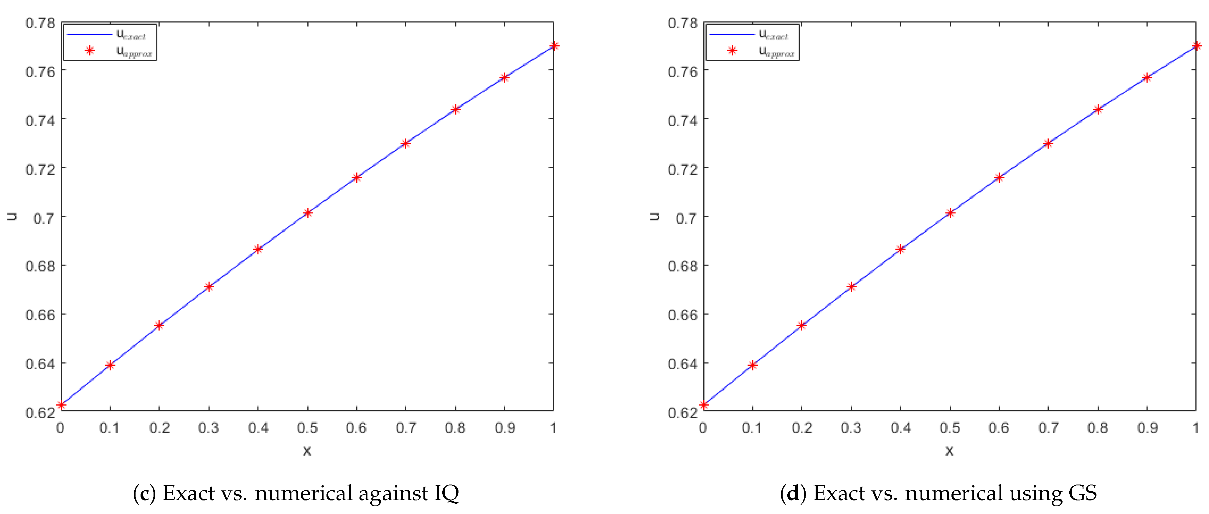
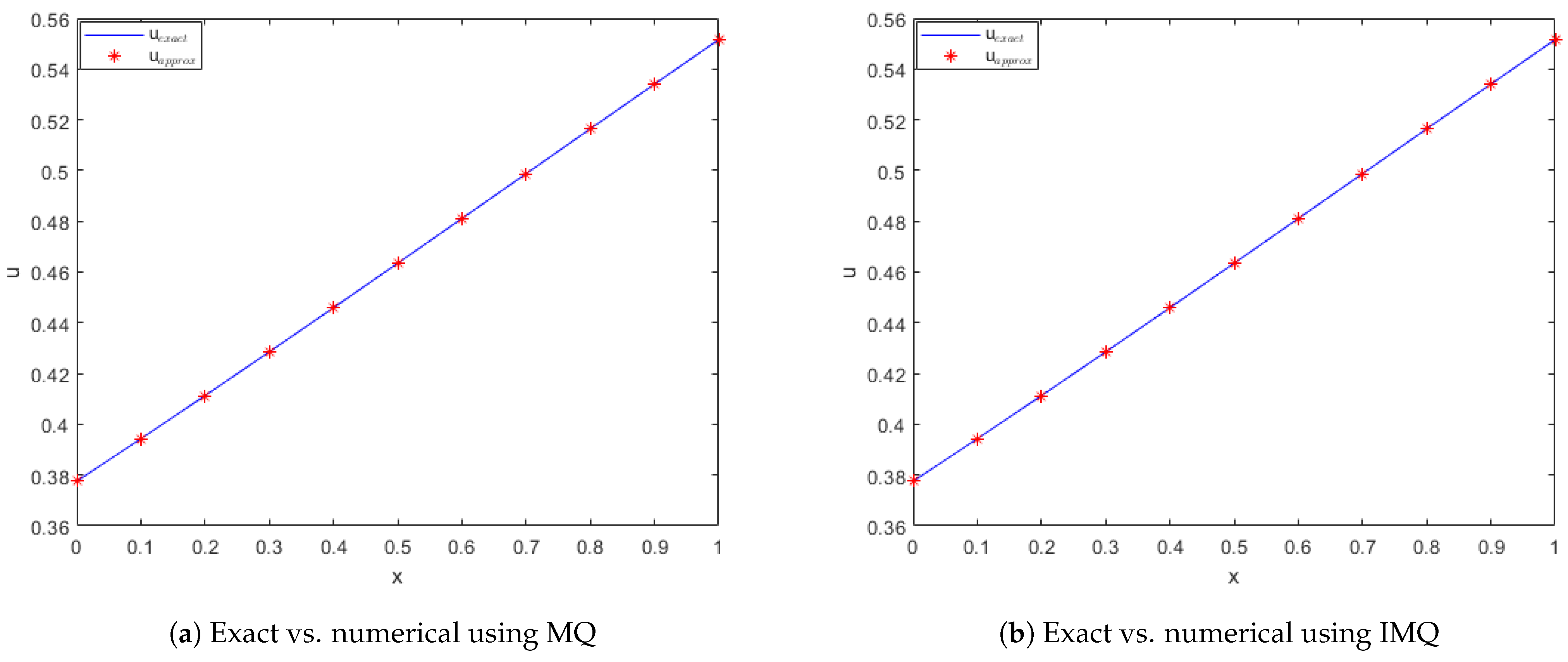
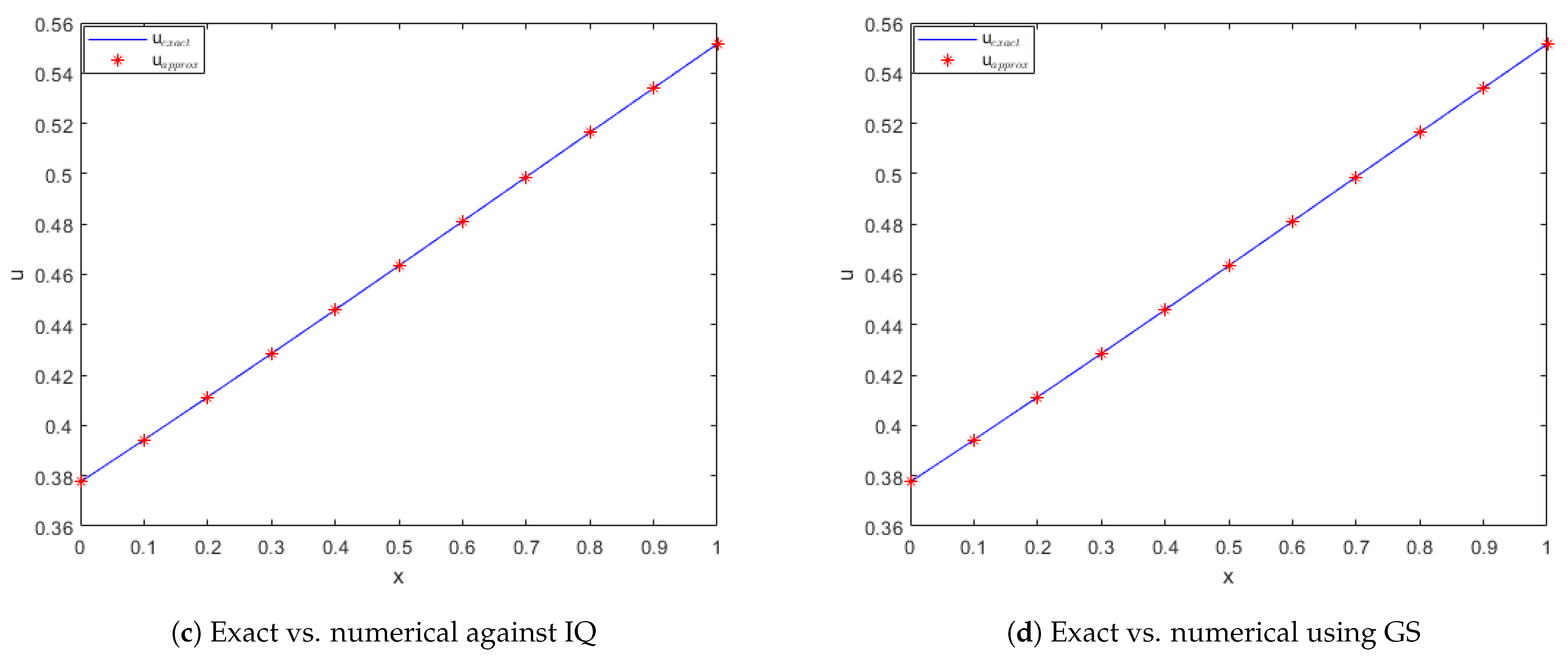
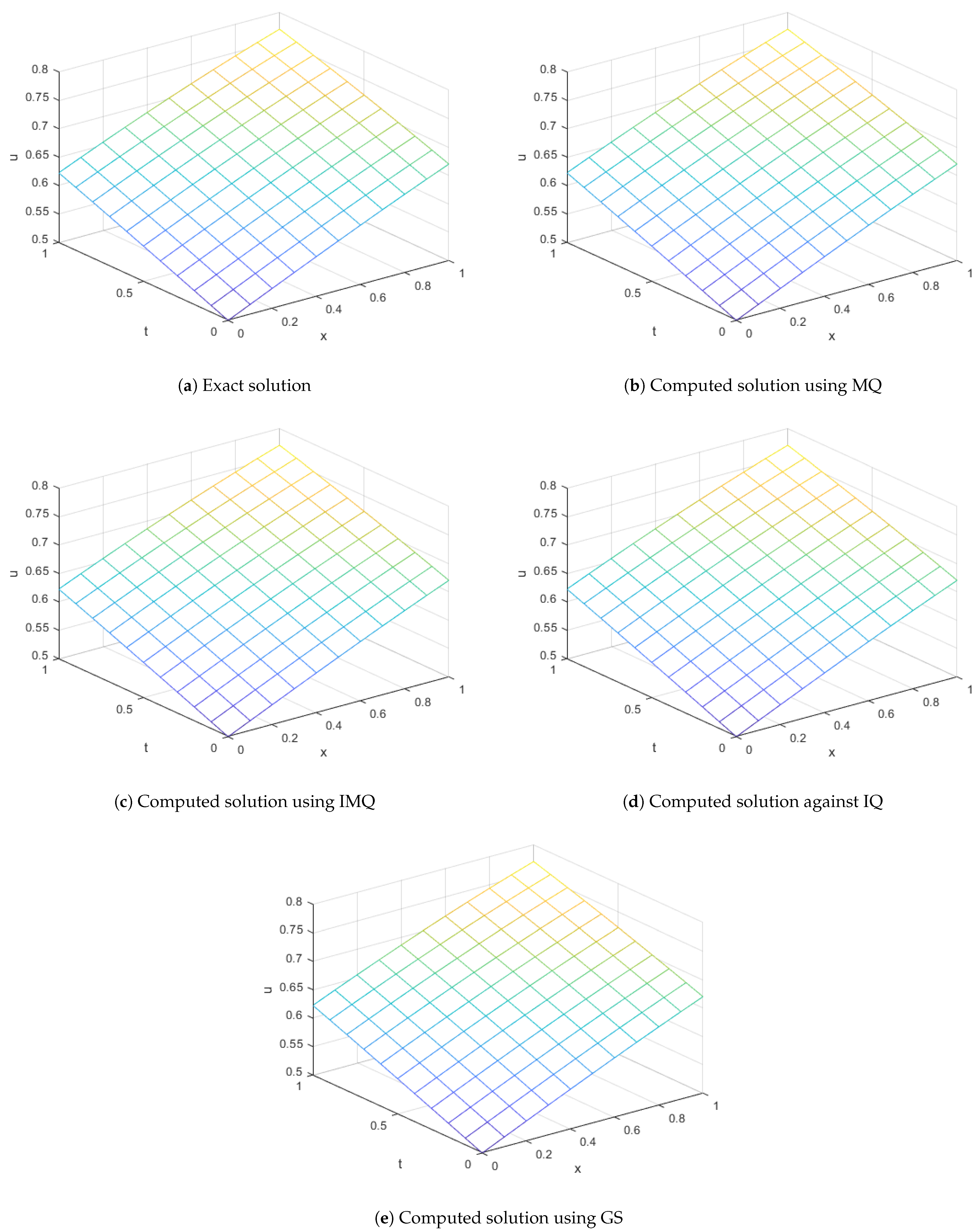
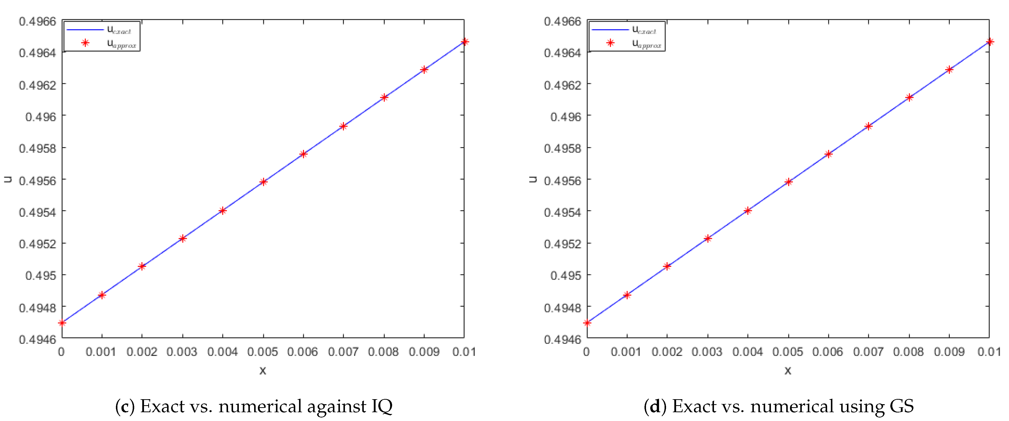
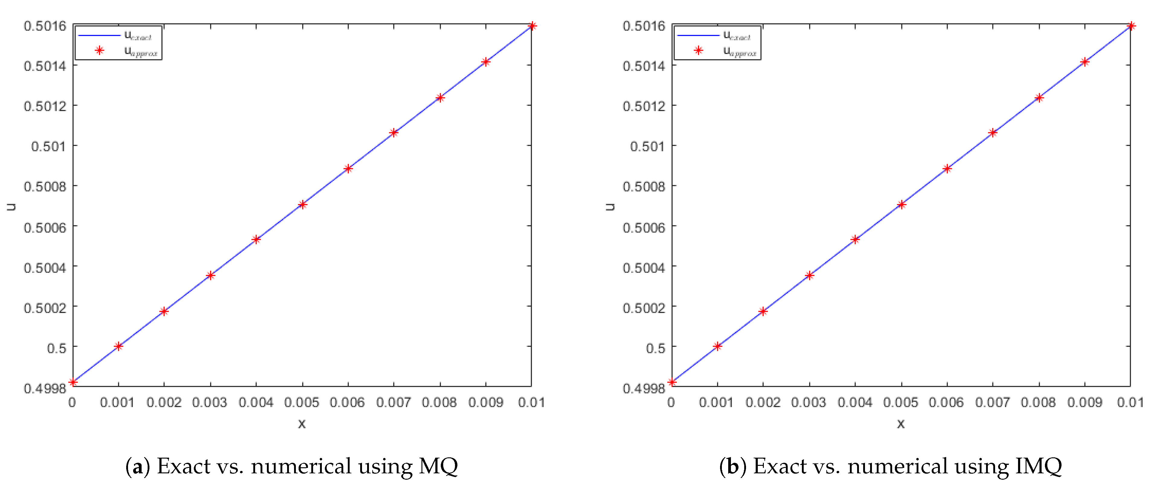
Figure 2.
Exact vs. computed solution corresponds to Example 1 when , using MQ, IMQ, IQ, and GS RBFs.
Figure 2.
Exact vs. computed solution corresponds to Example 1 when , using MQ, IMQ, IQ, and GS RBFs.
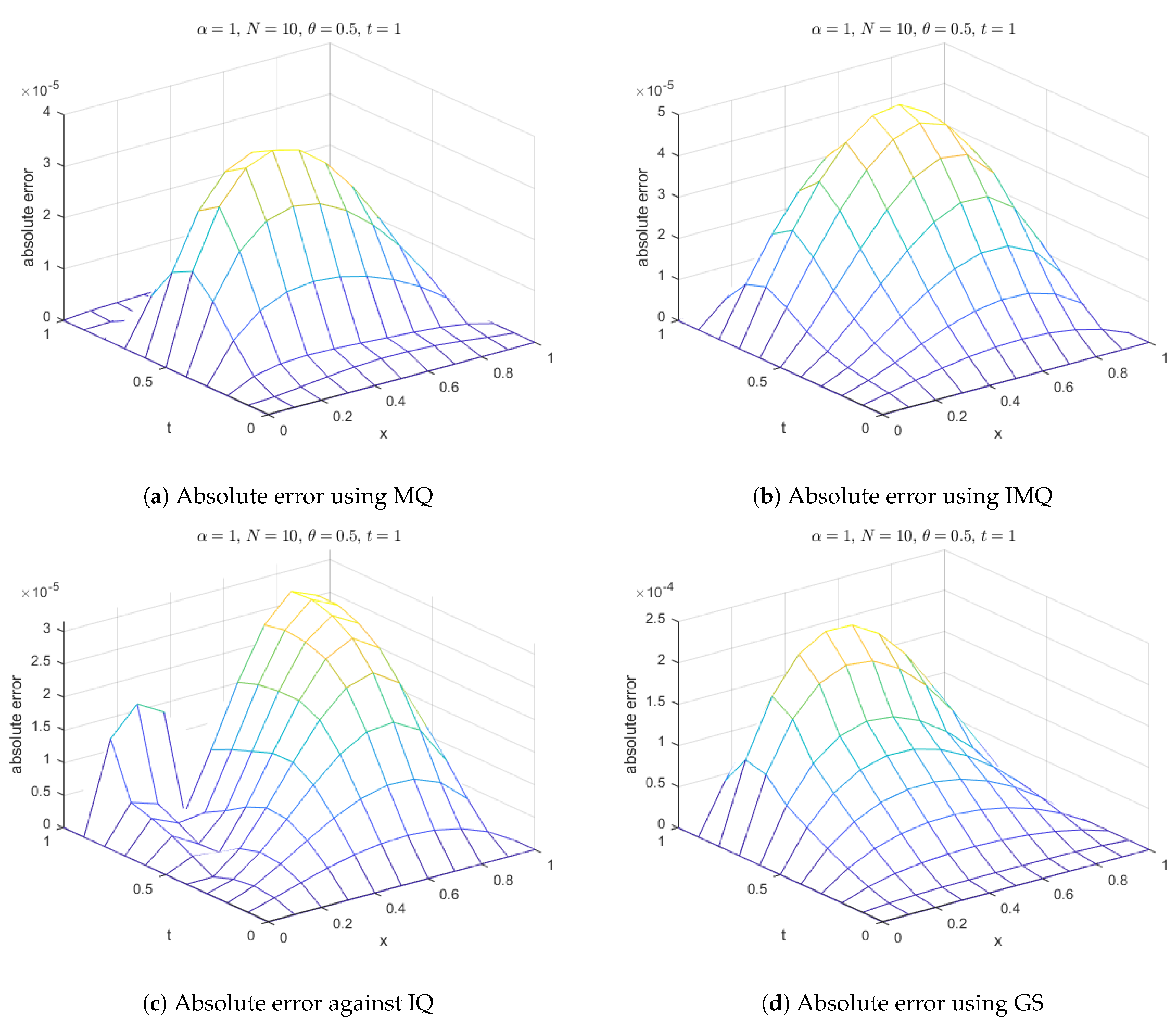
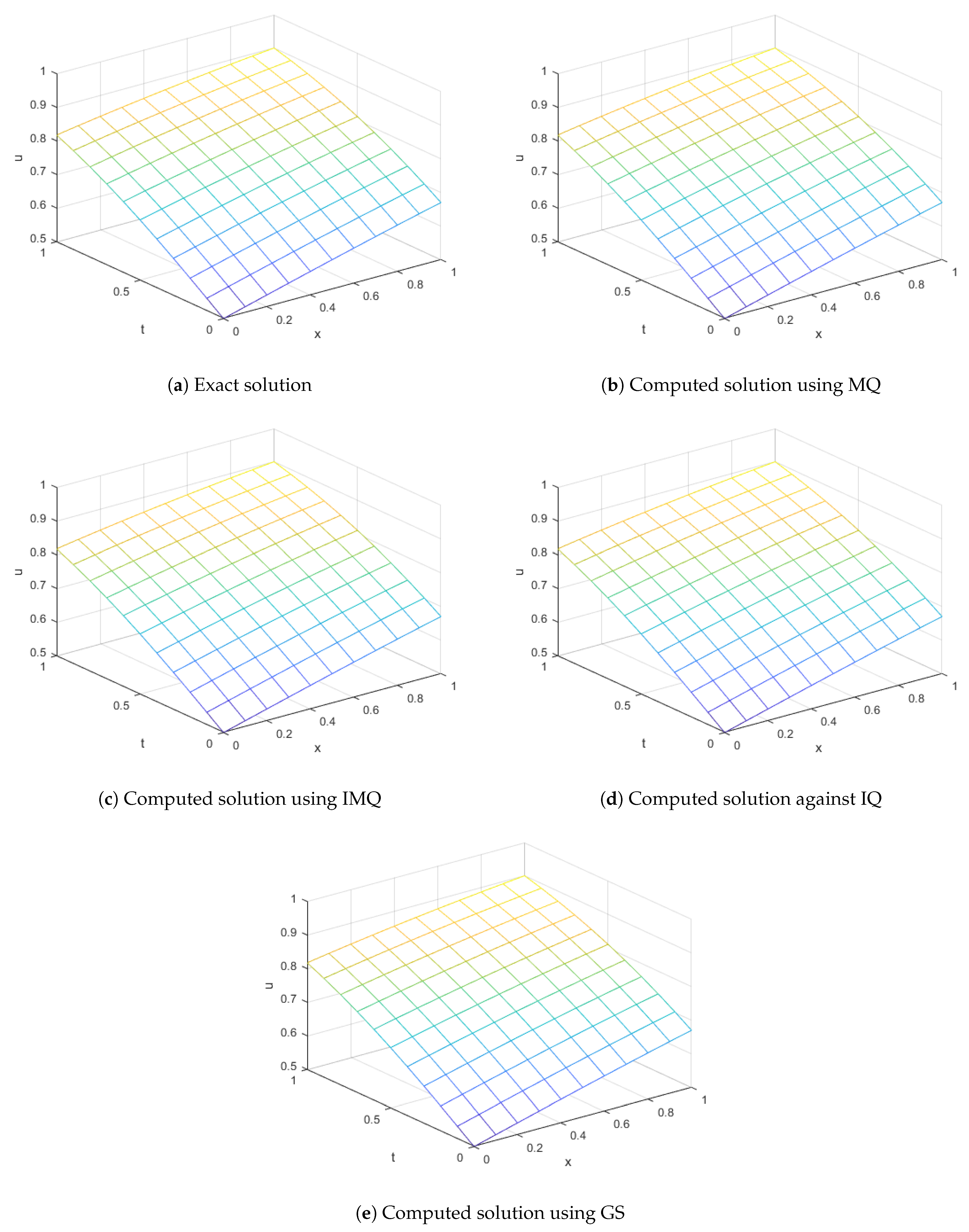
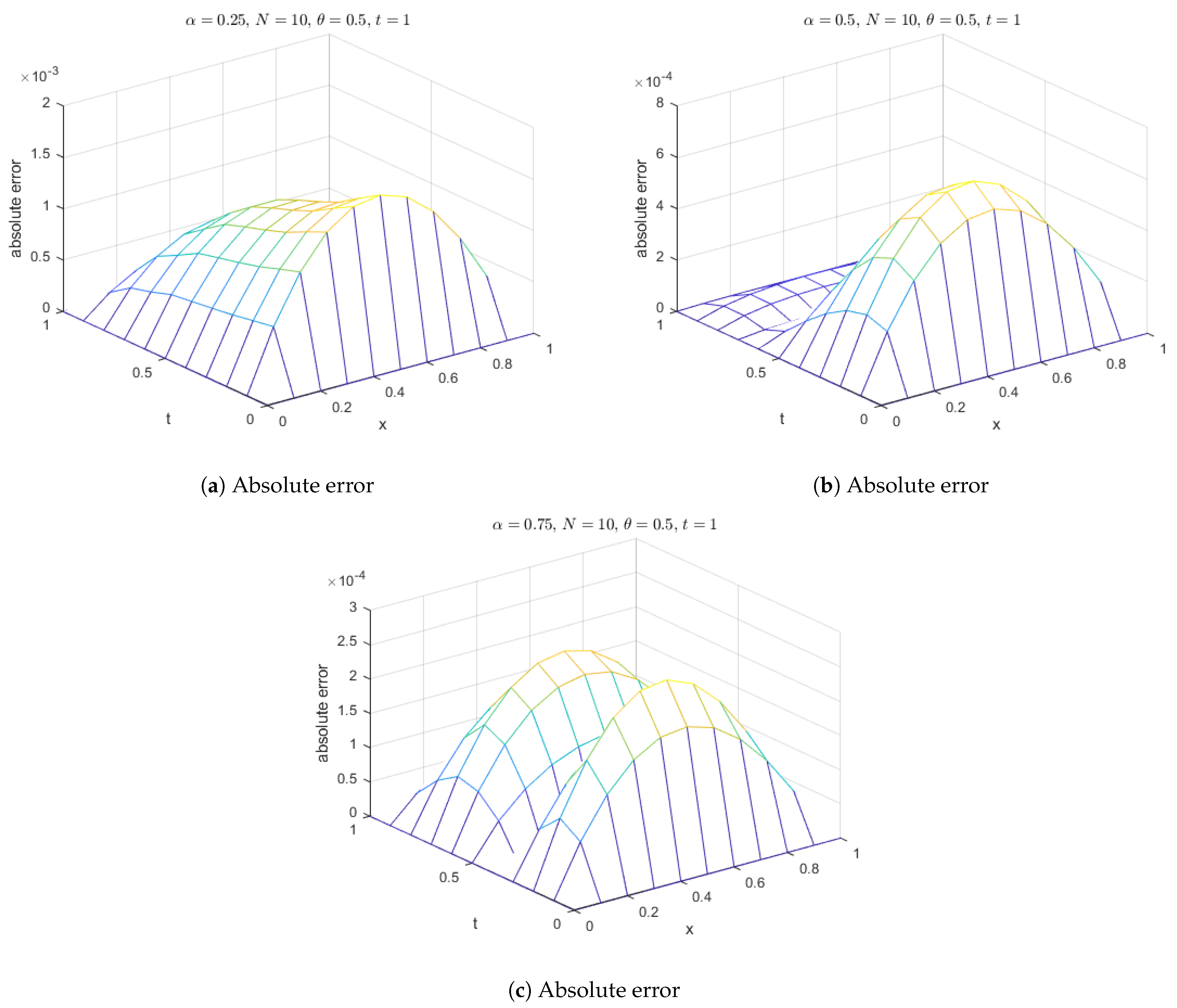
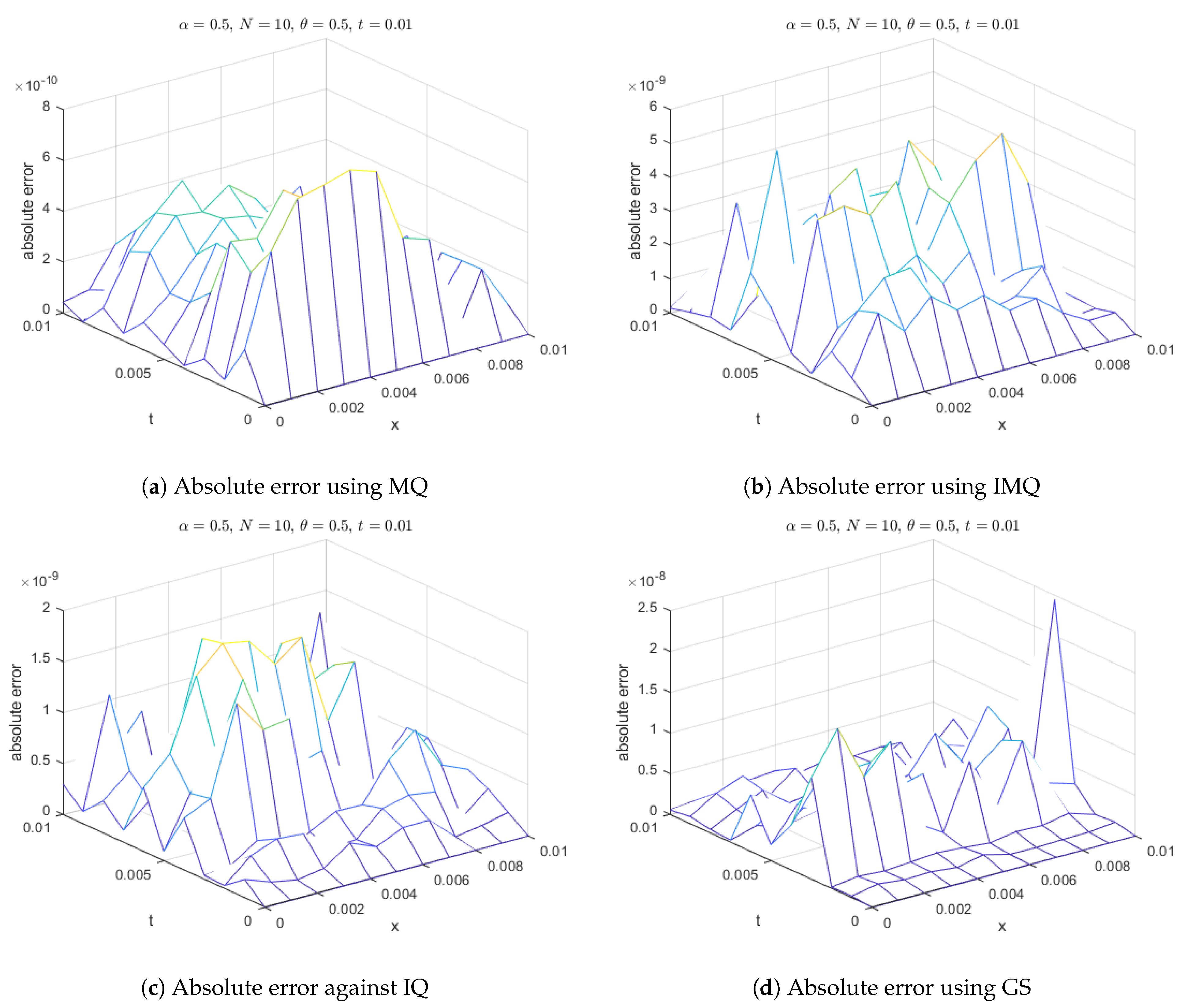
Figure 3.
Absolute error of MQ, IMQ, IQ, and GS at corresponds to Example 1.
Figure 3.
Absolute error of MQ, IMQ, IQ, and GS at corresponds to Example 1.
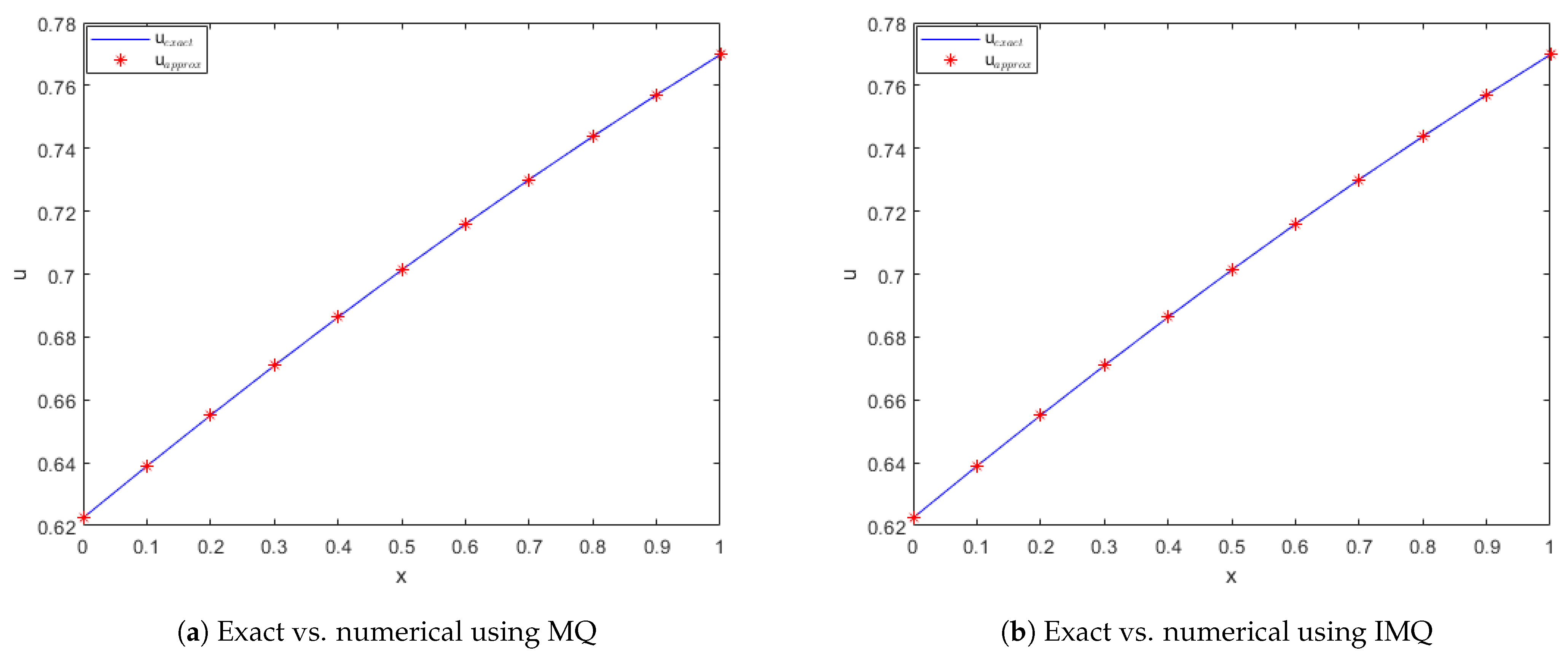
Figure 4.
Comparison of exact and computed solution corresponds to Example 1 at and using MQ, IMQ, IQ, and GS RBFs.
Figure 4.
Comparison of exact and computed solution corresponds to Example 1 at and using MQ, IMQ, IQ, and GS RBFs.
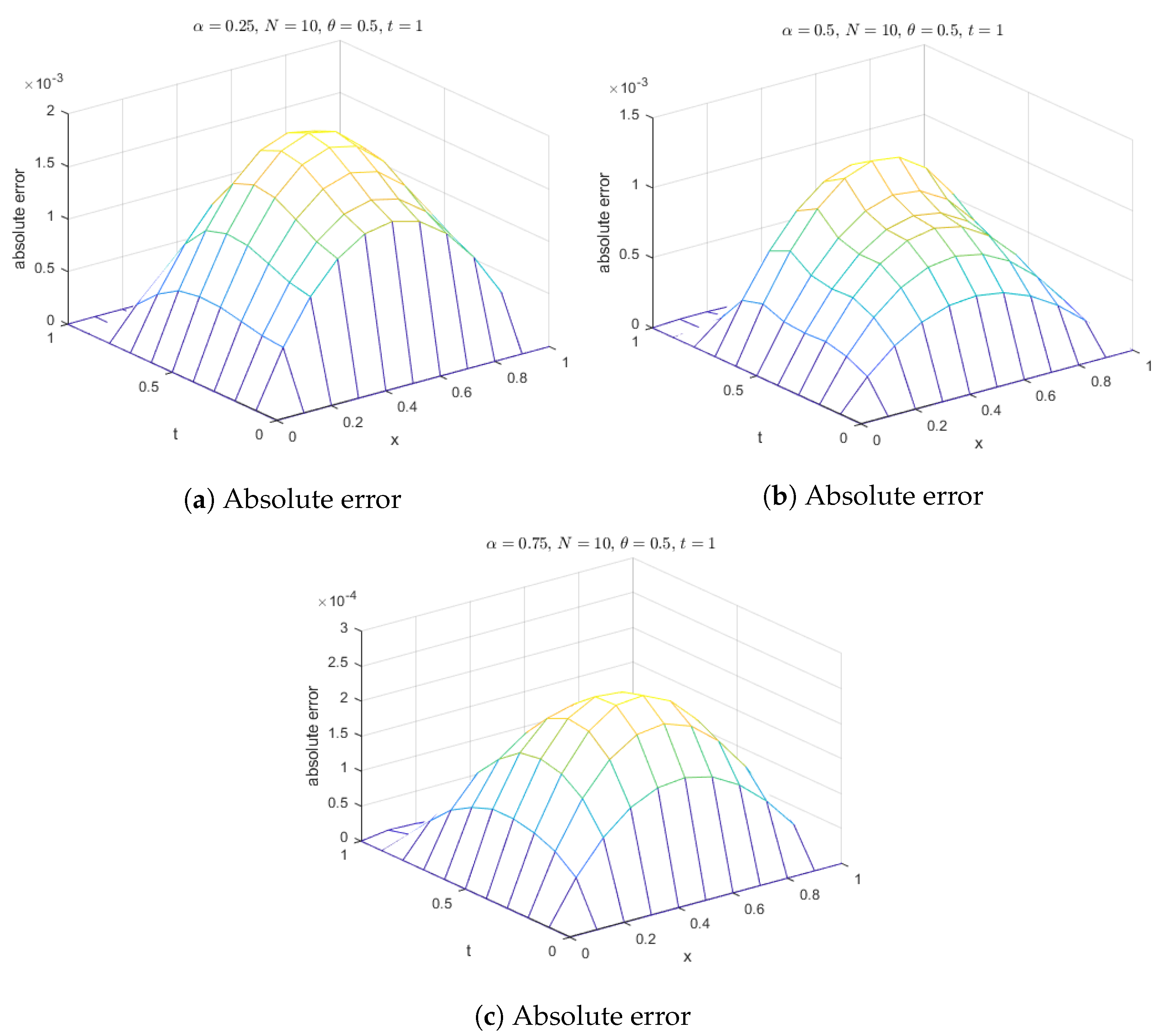
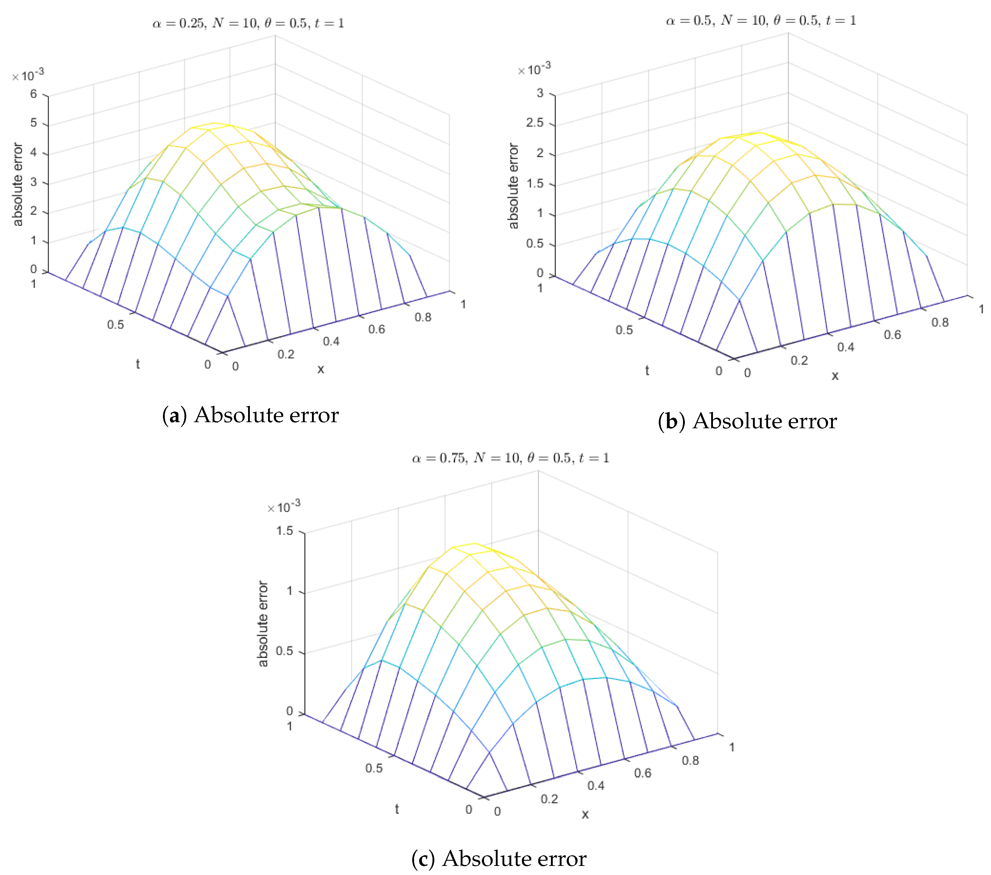
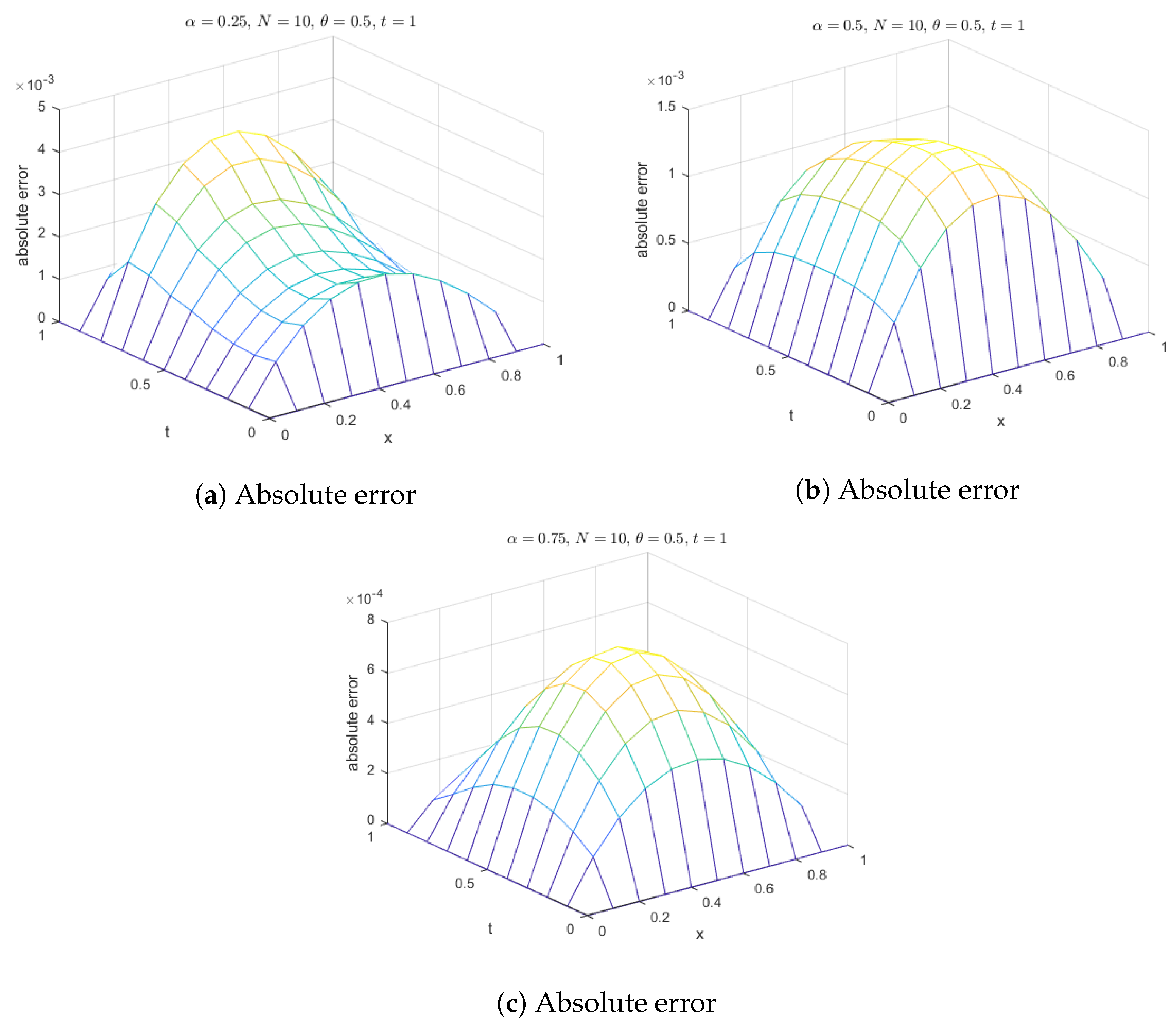
Figure 5.
Absolute errors for Example 1 with different values of ’s using MQ RBF.
Figure 5.
Absolute errors for Example 1 with different values of ’s using MQ RBF.
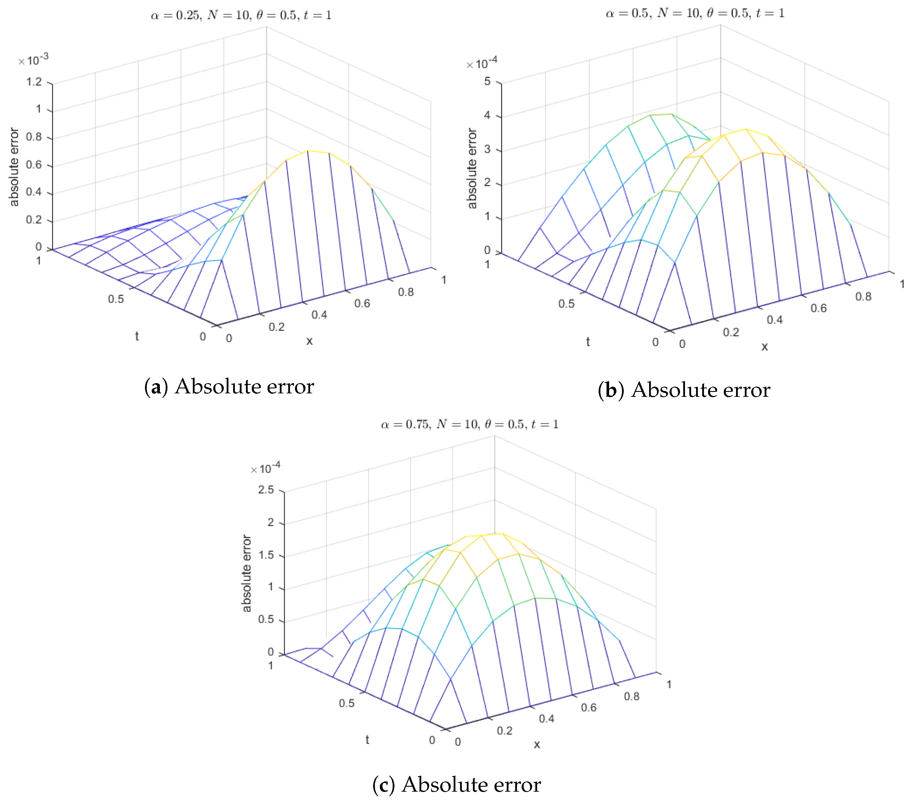
Figure 6.
Absolute errors for Example 1 with different values of ’s using IMQ RBF.
Figure 6.
Absolute errors for Example 1 with different values of ’s using IMQ RBF.
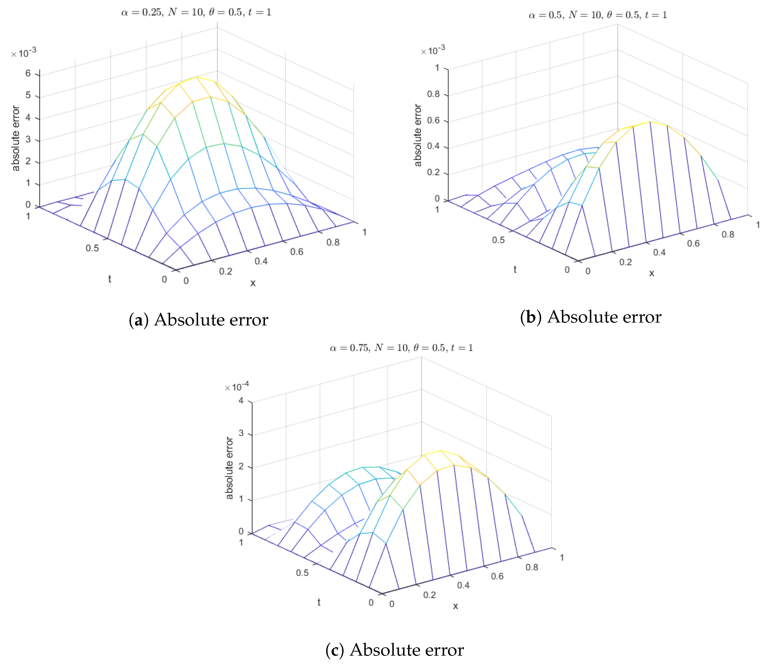
Figure 7.
Absolute errors for Example 1 with different values of ’s using IQ RBF.
Figure 7.
Absolute errors for Example 1 with different values of ’s using IQ RBF.
Figure 8.
Absolute errors for Example 1 with different values of ’s using GS RBF.
Figure 8.
Absolute errors for Example 1 with different values of ’s using GS RBF.
Figure 9.
Error norms and spectral radius correspond to Example 2 when , using MQ, IMQ, IQ, and GS RBFs.
Figure 9.
Error norms and spectral radius correspond to Example 2 when , using MQ, IMQ, IQ, and GS RBFs.
Figure 10.
Exact vs. computed solution corresponds to Example 2 when , using MQ, IMQ, IQ, and GS RBFs.
Figure 10.
Exact vs. computed solution corresponds to Example 2 when , using MQ, IMQ, IQ, and GS RBFs.
Figure 11.
Absolute error of MQ, IMQ, IQ, and GS at corresponds to Example 2.
Figure 11.
Absolute error of MQ, IMQ, IQ, and GS at corresponds to Example 2.
Figure 12.
Comparison of exact and computed solution corresponds to Example 2 at and using MQ, IMQ, IQ, and GS RBFs.
Figure 12.
Comparison of exact and computed solution corresponds to Example 2 at and using MQ, IMQ, IQ, and GS RBFs.
Figure 13.
Absolute errors for Example 3 with different values of ’s using MQ RBF.
Figure 13.
Absolute errors for Example 3 with different values of ’s using MQ RBF.
Figure 14.
Absolute errors for Example 3 with different values of ’s using IMQ RBF.
Figure 14.
Absolute errors for Example 3 with different values of ’s using IMQ RBF.
Figure 15.
Absolute errors for Example 3 with different values of ’s using IQ RBF.
Figure 15.
Absolute errors for Example 3 with different values of ’s using IQ RBF.
Figure 16.
Absolute errors for Example 3 with different values of ’s using GS RBF.
Figure 16.
Absolute errors for Example 3 with different values of ’s using GS RBF.
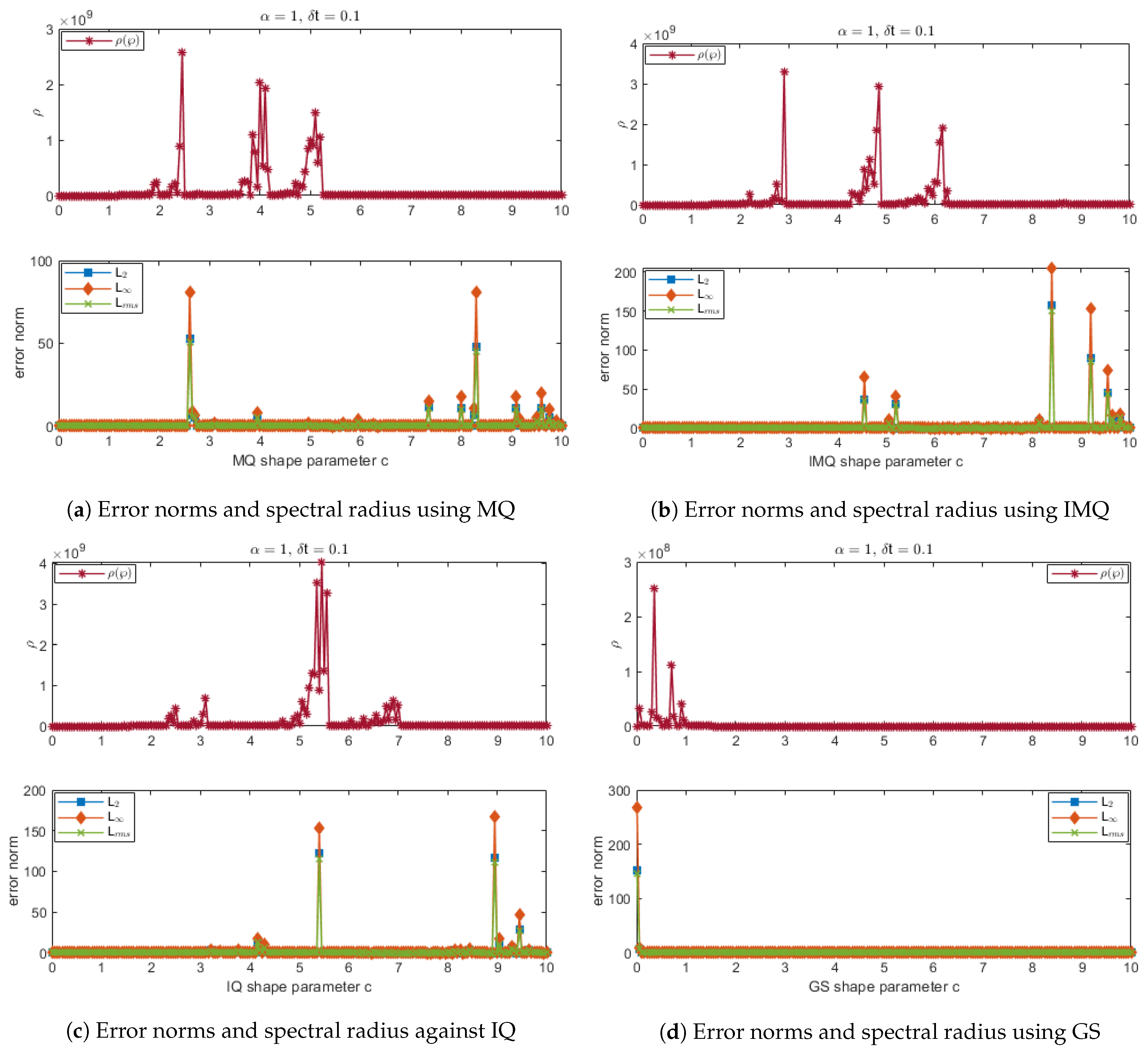
Figure 17.
Error norms and spectral radius correspond to Example 3 when , using MQ, IMQ, IQ, and GS RBFs.
Figure 17.
Error norms and spectral radius correspond to Example 3 when , using MQ, IMQ, IQ, and GS RBFs.
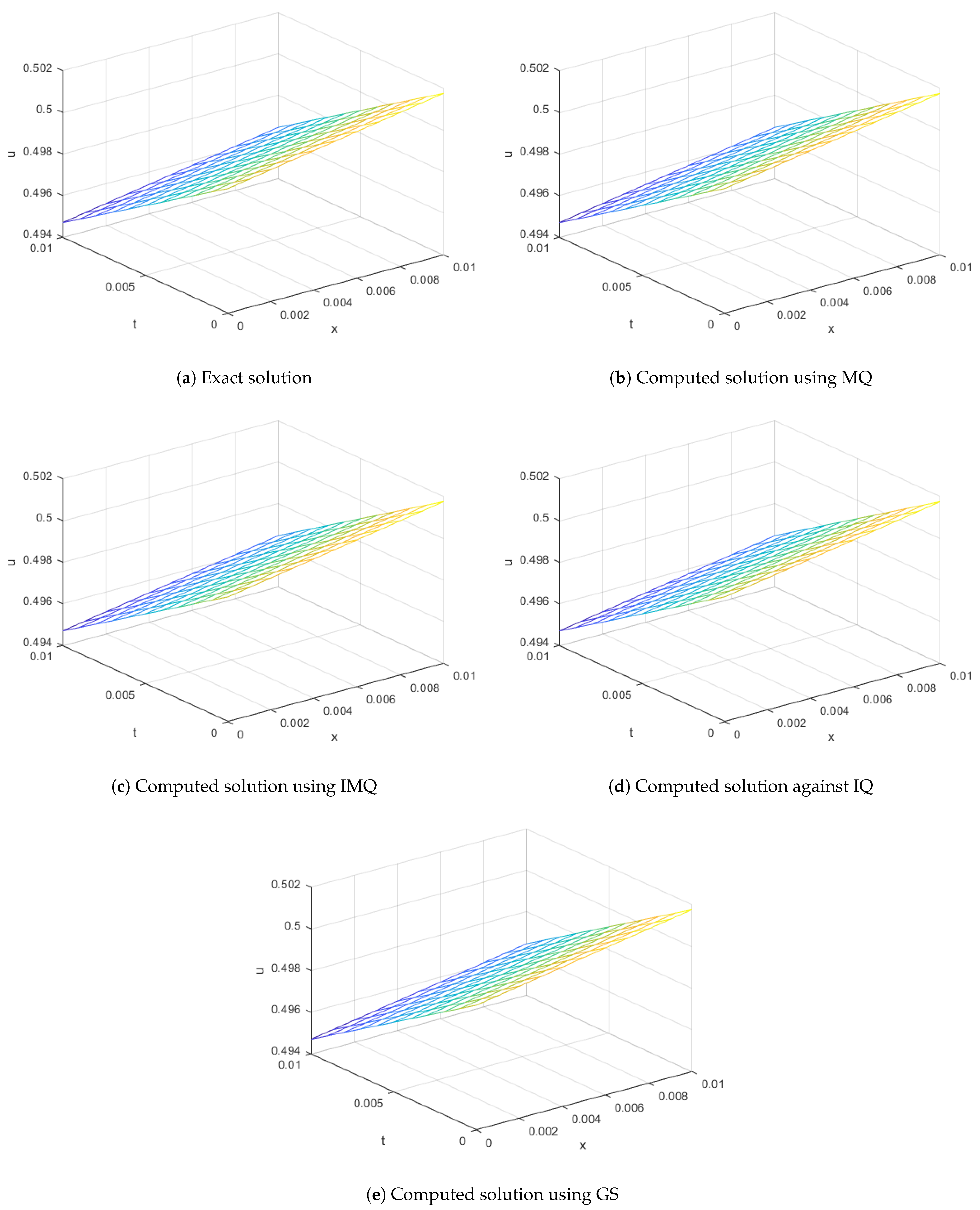
Figure 18.
Exact vs. computed solution corresponds to Example 3 when , using MQ, IMQ, IQ, and GS RBFs.
Figure 18.
Exact vs. computed solution corresponds to Example 3 when , using MQ, IMQ, IQ, and GS RBFs.
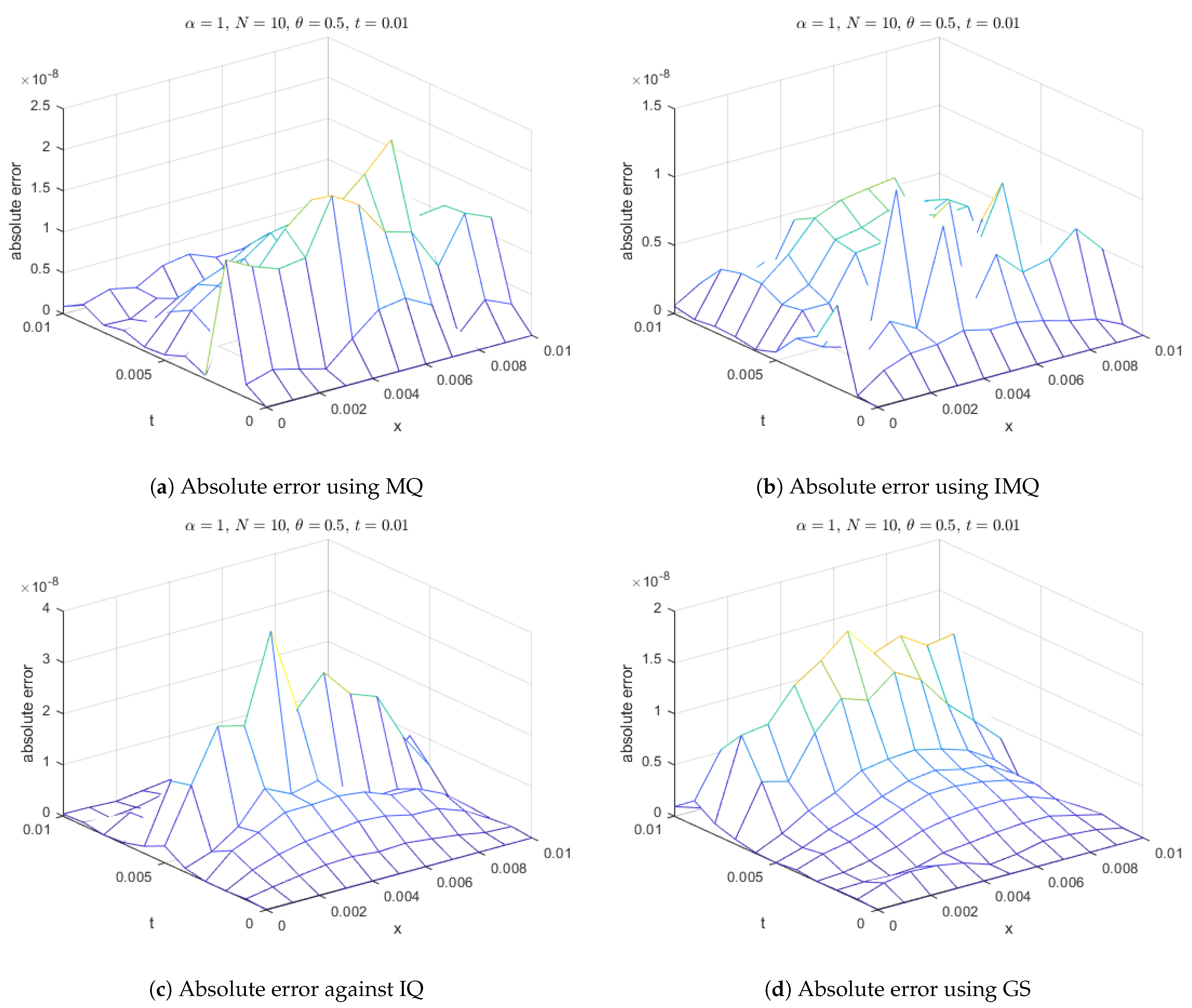
Figure 19.
Absolute error of MQ, IMQ, IQ, and GS at t = 1 × corresponds to Example 3.
Figure 19.
Absolute error of MQ, IMQ, IQ, and GS at t = 1 × corresponds to Example 3.
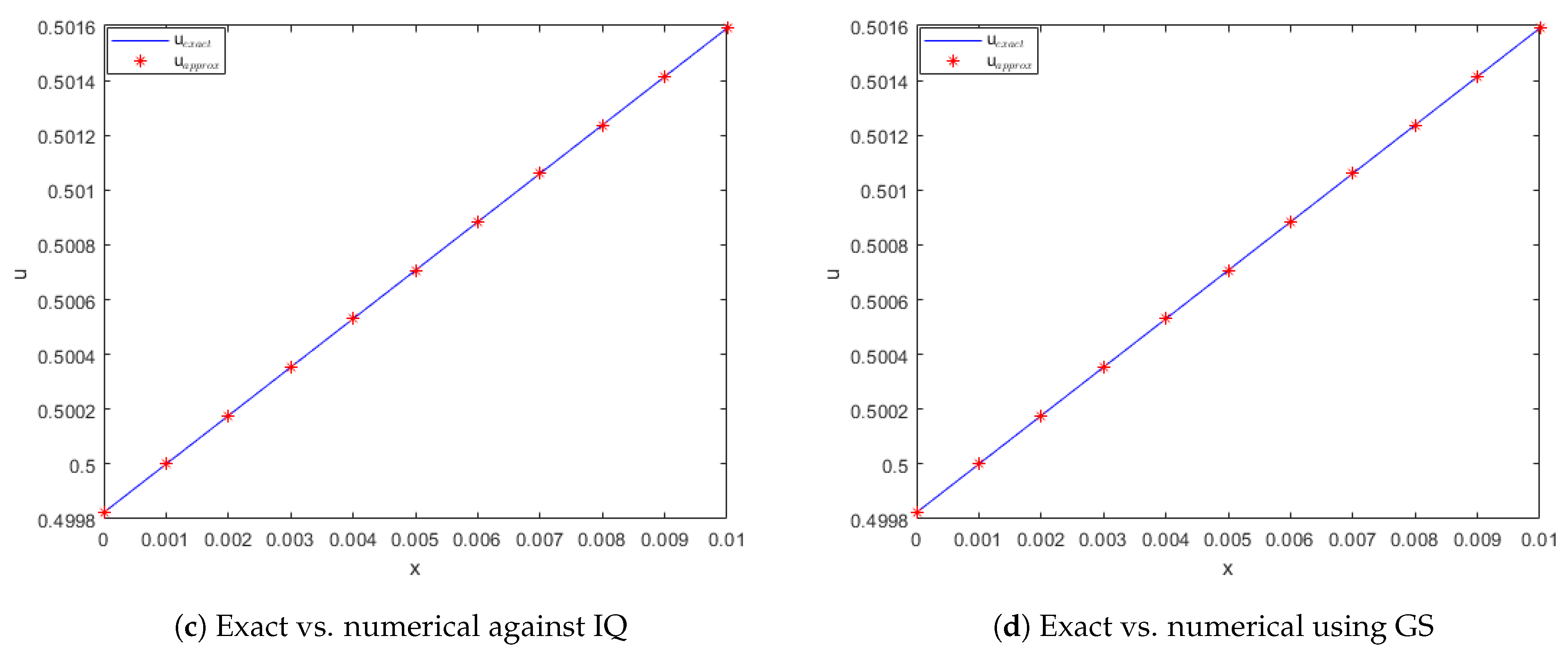
Figure 20.
Comparison of exact and computed solution corresponds to Example 3 at t = 1 × and using MQ, IMQ, IQ, and GS RBFs.
Figure 20.
Comparison of exact and computed solution corresponds to Example 3 at t = 1 × and using MQ, IMQ, IQ, and GS RBFs.
Figure 21.
Absolute errors for Example 3 with different values of ’s using MQ RBF.
Figure 21.
Absolute errors for Example 3 with different values of ’s using MQ RBF.
Figure 22.
Absolute errors for Example 3 with different values of ’s using IMQ RBF.
Figure 22.
Absolute errors for Example 3 with different values of ’s using IMQ RBF.
Figure 23.
Absolute errors for Example 3 with different values of ’s using IQ RBF.
Figure 23.
Absolute errors for Example 3 with different values of ’s using IQ RBF.
Figure 24.
Absolute errors for Example 3 with different values of ’s using GS RBF.
Figure 24.
Absolute errors for Example 3 with different values of ’s using GS RBF.
Figure 25.
Error norms and spectral radius correspond to Example 4 when , using MQ, IMQ, IQ, and GS RBFs.
Figure 25.
Error norms and spectral radius correspond to Example 4 when , using MQ, IMQ, IQ, and GS RBFs.
Figure 26.
Error norms and spectral radius correspond to Example 4 when , using MQ, IMQ, IQ, and GS RBFs.
Figure 26.
Error norms and spectral radius correspond to Example 4 when , using MQ, IMQ, IQ, and GS RBFs.
Figure 27.
Exact vs. computed solution corresponds to Example 4 when , using MQ, IMQ, IQ, and GS RBFs.
Figure 27.
Exact vs. computed solution corresponds to Example 4 when , using MQ, IMQ, IQ, and GS RBFs.
Figure 28.
Exact vs. computed solution corresponds to Example 4 when , using MQ, IMQ, IQ, and GS RBFs.
Figure 28.
Exact vs. computed solution corresponds to Example 4 when , using MQ, IMQ, IQ, and GS RBFs.
Figure 29.
Absolute error of MQ, IMQ, IQ, and GS at corresponds to Example 4.
Figure 29.
Absolute error of MQ, IMQ, IQ, and GS at corresponds to Example 4.
Figure 30.
Absolute error of MQ, IMQ, IQ, and GS at corresponds to Example 4.
Figure 30.
Absolute error of MQ, IMQ, IQ, and GS at corresponds to Example 4.
Figure 31.
Comparison of exact and computed solution corresponds to Example 4 at and using MQ, IMQ, IQ, and GS RBFs.
Figure 31.
Comparison of exact and computed solution corresponds to Example 4 at and using MQ, IMQ, IQ, and GS RBFs.
Figure 32.
Comparison of exact and computed solution corresponds to Example 4 at t = 0.01 and α = 0.5 using MQ, IMQ, IQ, and GS RBFs.
Figure 32.
Comparison of exact and computed solution corresponds to Example 4 at t = 0.01 and α = 0.5 using MQ, IMQ, IQ, and GS RBFs.
Table 1.
Comparison of computed values of the present method solution with FRDTM using MQ, IMQ, IQ, and GS RBFs for , , , , and corresponds to Example 1.
Table 1.
Comparison of computed values of the present method solution with FRDTM using MQ, IMQ, IQ, and GS RBFs for , , , , and corresponds to Example 1.
| Exact | | |
|---|
| [25] | MQ | IMQ | IQ | GS | [25] | MQ | IMQ | IQ | GS |
|---|
| | | | | | | |
|---|
| (0.1, 0.2) | 0.492678 | 0.427418 | 0.492029 | 0.492126 | 0.492364 | 0.492466 | 0.454935 | 0.492344 | 0.492386 | 0.492489 | 0.492564 |
| (0.1, 0.4) | 0.467723 | 0.411555 | 0.467129 | 0.467083 | 0.467582 | 0.467632 | 0.429688 | 0.467279 | 0.467401 | 0.467571 | 0.467645 |
| (0.1, 0.6) | 0.442927 | 0.401291 | 0.443115 | 0.442313 | 0.442917 | 0.442952 | 0.410894 | 0.442364 | 0.442535 | 0.442858 | 0.442910 |
| (0.1, 0.8) | 0.418414 | 0.393583 | 0.418856 | 0.418114 | 0.418463 | 0.418448 | 0.395550 | 0.418125 | 0.418259 | 0.418442 | 0.418426 |
| (0.3, 0.2) | 0.528004 | 0.461640 | 0.526474 | 0.526698 | 0.527298 | 0.527493 | 0.489905 | 0.527223 | 0.527325 | 0.527585 | 0.527735 |
| (0.3, 0.4) | 0.503033 | 0.445267 | 0.501595 | 0.501492 | 0.502762 | 0.502797 | 0.464133 | 0.501982 | 0.502252 | 0.502729 | 0.502842 |
| (0.3, 0.6) | 0.478047 | 0.434619 | 0.478461 | 0.476553 | 0.478071 | 0.478089 | 0.444777 | 0.476697 | 0.477079 | 0.477948 | 0.477992 |
| (0.3, 0.8) | 0.453171 | 0.426595 | 0.454236 | 0.452429 | 0.453300 | 0.453249 | 0.428860 | 0.452424 | 0.452737 | 0.453293 | 0.453186 |
| (0.5, 0.2) | 0.563051 | 0.496159 | 0.561223 | 0.561488 | 0.562257 | 0.562434 | 0.524966 | 0.562128 | 0.562253 | 0.562589 | 0.562736 |
| (0.5, 0.4) | 0.538313 | 0.479367 | 0.536561 | 0.536435 | 0.538071 | 0.538014 | 0.498899 | 0.537055 | 0.537363 | 0.538023 | 0.538083 |
| (0.5, 0.6) | 0.513385 | 0.468375 | 0.513874 | 0.511551 | 0.513484 | 0.513427 | 0.479131 | 0.511752 | 0.512181 | 0.513354 | 0.513312 |
| (0.5, 0.8) | 0.488390 | 0.460051 | 0.489708 | 0.487477 | 0.488573 | 0.488485 | 0.462744 | 0.487455 | 0.487818 | 0.488617 | 0.488400 |
| (0.7, 0.2) | 0.597480 | 0.530655 | 0.595947 | 0.596167 | 0.596862 | 0.596963 | 0.559780 | 0.596717 | 0.596823 | 0.597129 | 0.597225 |
| (0.7, 0.4) | 0.573214 | 0.513551 | 0.571727 | 0.571609 | 0.573089 | 0.572956 | 0.533657 | 0.572160 | 0.572409 | 0.573040 | 0.573026 |
| (0.7, 0.6) | 0.548590 | 0.502269 | 0.549021 | 0.547016 | 0.548741 | 0.548627 | 0.513645 | 0.547210 | 0.547543 | 0.548648 | 0.548530 |
| (0.7, 0.8) | 0.523726 | 0.493674 | 0.524882 | 0.522951 | 0.523912 | 0.523812 | 0.496910 | 0.522935 | 0.523224 | 0.523996 | 0.523734 |
| (0.9, 0.2) | 0.630974 | 0.564813 | 0.630322 | 0.630415 | 0.630735 | 0.630756 | 0.594013 | 0.630655 | 0.630700 | 0.630843 | 0.630870 |
| (0.9, 0.4) | 0.607400 | 0.547522 | 0.606766 | 0.606706 | 0.607385 | 0.607291 | 0.568079 | 0.606954 | 0.607057 | 0.607361 | 0.607325 |
| (0.9, 0.6) | 0.583315 | 0.536019 | 0.583518 | 0.582633 | 0.583413 | 0.583335 | 0.548003 | 0.582725 | 0.582855 | 0.583381 | 0.583293 |
| (0.9, 0.8) | 0.558825 | 0.527198 | 0.559346 | 0.558498 | 0.558922 | 0.558867 | 0.531062 | 0.558499 | 0.558612 | 0.558979 | 0.558831 |
Table 2.
Comparison of computed values of the present method solution with FRDTM using MQ, IMQ, IQ, and GS RBFs for , , , , and corresponds to Example 1.
Table 2.
Comparison of computed values of the present method solution with FRDTM using MQ, IMQ, IQ, and GS RBFs for , , , , and corresponds to Example 1.
| Exact | | |
|---|
| [25] | MQ | IMQ | IQ | GS | [25] | MQ | IMQ | IQ | GS |
|---|
| | | | | | | |
|---|
| (0.1, 0.2) | 0.492678 | 0.477029 | 0.492540 | 0.492594 | 0.492594 | 0.492630 | 0.492678 | 0.492674 | 0.492676 | 0.492674 | 0.492666 |
| (0.1, 0.4) | 0.467723 | 0.449555 | 0.467487 | 0.467619 | 0.467623 | 0.467672 | 0.467722 | 0.467706 | 0.467716 | 0.467707 | 0.467642 |
| (0.1, 0.6) | 0.442927 | 0.425857 | 0.442690 | 0.442835 | 0.442856 | 0.442912 | 0.442927 | 0.442909 | 0.442918 | 0.442905 | 0.442841 |
| (0.1, 0.8) | 0.418414 | 0.404564 | 0.418328 | 0.418368 | 0.418407 | 0.418433 | 0.418416 | 0.418407 | 0.418406 | 0.418399 | 0.418391 |
| (0.3, 0.2) | 0.528004 | 0.512307 | 0.527682 | 0.527809 | 0.527819 | 0.527892 | 0.528003 | 0.527996 | 0.528000 | 0.527994 | 0.527975 |
| (0.3, 0.4) | 0.503033 | 0.484582 | 0.502475 | 0.502807 | 0.502828 | 0.502912 | 0.503030 | 0.502996 | 0.503019 | 0.502999 | 0.502881 |
| (0.3, 0.6) | 0.478047 | 0.460446 | 0.477457 | 0.477869 | 0.477926 | 0.478004 | 0.478035 | 0.478003 | 0.478026 | 0.477996 | 0.477887 |
| (0.3, 0.8) | 0.453171 | 0.438573 | 0.452937 | 0.453093 | 0.453193 | 0.453211 | 0.453136 | 0.453156 | 0.453153 | 0.453136 | 0.453114 |
| (0.5, 0.2) | 0.563051 | 0.547464 | 0.562671 | 0.562826 | 0.562848 | 0.562922 | 0.563051 | 0.563043 | 0.563047 | 0.563041 | 0.563015 |
| (0.5, 0.4) | 0.538313 | 0.519760 | 0.537643 | 0.538070 | 0.53811 | 0.538172 | 0.538308 | 0.53827 | 0.538298 | 0.538274 | 0.538165 |
| (0.5, 0.6) | 0.513385 | 0.495415 | 0.512658 | 0.513228 | 0.513305 | 0.513335 | 0.513362 | 0.513331 | 0.513361 | 0.513326 | 0.513249 |
| (0.5, 0.8) | 0.488390 | 0.473159 | 0.488089 | 0.488345 | 0.488474 | 0.488438 | 0.488322 | 0.488375 | 0.488370 | 0.488348 | 0.488328 |
| (0.7, 0.2) | 0.597480 | 0.582153 | 0.597165 | 0.597300 | 0.597326 | 0.597377 | 0.597479 | 0.597474 | 0.597477 | 0.597471 | 0.597446 |
| (0.7, 0.4) | 0.573214 | 0.554743 | 0.572650 | 0.573038 | 0.573084 | 0.573102 | 0.573207 | 0.573178 | 0.573202 | 0.573181 | 0.573113 |
| (0.7, 0.6) | 0.548590 | 0.530429 | 0.547972 | 0.548512 | 0.548585 | 0.548554 | 0.548558 | 0.548544 | 0.548571 | 0.548541 | 0.548522 |
| (0.7, 0.8) | 0.523726 | 0.508002 | 0.523469 | 0.523735 | 0.523852 | 0.523770 | 0.523629 | 0.523715 | 0.523709 | 0.523691 | 0.523680 |
| (0.9, 0.2) | 0.630974 | 0.616050 | 0.630841 | 0.630902 | 0.630917 | 0.630933 | 0.630973 | 0.630971 | 0.630972 | 0.630970 | 0.630957 |
| (0.9, 0.4) | 0.607400 | 0.589194 | 0.607160 | 0.607341 | 0.607365 | 0.607357 | 0.607392 | 0.607384 | 0.607395 | 0.607386 | 0.607368 |
| (0.9, 0.6) | 0.583315 | 0.565149 | 0.583053 | 0.583308 | 0.583343 | 0.583305 | 0.583277 | 0.583296 | 0.583307 | 0.583294 | 0.583305 |
| (0.9, 0.8) | 0.558825 | 0.542773 | 0.558721 | 0.558852 | 0.558906 | 0.558848 | 0.558707 | 0.558822 | 0.558818 | 0.558811 | 0.558809 |
Table 3.
Error norms at various time levels using MQ, IMQ, IQ, and GS RBFs for , , , , and corresponds to Example 1.
Table 3.
Error norms at various time levels using MQ, IMQ, IQ, and GS RBFs for , , , , and corresponds to Example 1.
| RBFs | t | | |
|---|
| | | | | |
|---|
| MQ | | | |
| 0.2 | 1.331 × | 1.828 × | 1.270 × | 6.715 × | 9.231 × | 6.402 × |
| 0.4 | 1.272 × | 1.752 × | 1.213 × | 9.153 × | 1.259 × | 8.727 × |
| 0.6 | 3.663 × | 4.893 × | 3.493 × | 1.187 × | 1.633 × | 1.132 × |
| 0.8 | 9.663 × | 1.318 × | 9.214 × | 6.701 × | 9.350 × | 6.389 × |
| 1 | 4.238 × | 7.006 × | 4.041 × | 7.414 × | 1.297 × | 7.069 × |
| IMQ | | | |
| 0.2 | 1.138 × | 1.563 × | 1.085 × | 5.811 × | 7.983 × | 5.541 × |
| 0.4 | 1.368 × | 1.879 × | 1.304 × | 6.897 × | 9.504 × | 6.576 × |
| 0.6 | 1.334 × | 1.835 × | 1.272 × | 8.769 × | 1.204 × | 8.360 × |
| 0.8 | 6.601 × | 9.134 × | 6.294 × | 4.089 × | 5.721 × | 3.899 × |
| 1 | 1.199 × | 1.851 × | 1.143 × | 5.718 × | 9.971 × | 5.452 × |
| IQ | | | |
| 0.2 | 5.766 × | 7.940 × | 5.498 × | 3.359 × | 4.623 × | 3.202 × |
| 0.4 | 1.825 × | 2.724 × | 1.740 × | 2.147 × | 3.145 × | 2.047 × |
| 0.6 | 9.193 × | 1.510 × | 8.765 × | 6.746 × | 1.006 × | 6.432 × |
| 0.8 | 1.387 × | 1.929 × | 1.322 × | 1.804 × | 2.700 × | 1.720 × |
| 1 | 5.465 × | 8.804 × | 5.211 × | 3.988 × | 6.707 × | 3.803 × |
| GS | | | |
| 0.2 | 4.473 × | 6.166 × | 4.265 × | 2.279 × | 3.146 × | 2.173 × |
| 0.4 | 2.152 × | 2.992 × | 2.052 × | 1.651 × | 2.302 × | 1.574 × |
| 0.6 | 3.447 × | 4.323 × | 3.286 × | 5.054 × | 7.298 × | 4.819 × |
| 0.8 | 7.107 × | 9.455 × | 6.776 × | 1.058 × | 1.617 × | 1.009 × |
| 1 | 4.706 × | 7.906 × | 4.487 × | 4.625 × | 8.048 × | 4.410 × |
Table 4.
Error norms at various time levels using MQ, IMQ, IQ, and GS RBFs for , , , , and corresponds to Example 1.
Table 4.
Error norms at various time levels using MQ, IMQ, IQ, and GS RBFs for , , , , and corresponds to Example 1.
| RBFs | t | | |
|---|
| | | | | |
|---|
| MQ | | | |
| 0.2 | 2.769 × | 3.802 × | 2.640 × | 5.932 × | 8.084 × | 5.656 × |
| 0.4 | 4.878 × | 6.702 × | 4.651 × | 3.153 × | 4.263 × | 3.006 × |
| 0.6 | 5.258 × | 7.275 × | 5.013 × | 3.904 × | 5.393 × | 3.722 × |
| 0.8 | 2.143 × | 3.014 × | 2.044 × | 1.143 × | 1.609 × | 1.090 × |
| 1 | 4.401 × | 6.944 × | 4.196 × | 7.107 × | 1.410 × | 6.776 × |
| IMQ | | | |
| 0.2 | 1.630 × | 2.249 × | 1.554 × | 2.886 × | 3.898 × | 2.751 × |
| 0.4 | 1.759 × | 2.466 × | 1.678 × | 1.103 × | 1.490 × | 1.052 × |
| 0.6 | 1.191 × | 1.785 × | 1.135 × | 1.739 × | 2.373 × | 1.658 × |
| 0.8 | 4.659 × | 7.766 × | 4.442 × | 1.510 × | 2.085 × | 1.440 × |
| 1 | 4.166 × | 6.616 × | 3.972 × | 4.264 × | 6.996 × | 4.065 × |
| IQ | | | |
| 0.2 | 1.476 × | 2.032 × | 1.407 × | 7.689 × | 1.021 × | 7.331 × |
| 0.4 | 1.489 × | 2.155 × | 1.420 × | 2.877 × | 3.894 × | 2.743 × |
| 0.6 | 7.313 × | 1.212 × | 6.972 × | 4.352 × | 5.947 × | 4.149 × |
| 0.8 | 7.707 × | 1.263 × | 7.349 × | 3.045 × | 4.238 × | 2.903 × |
| 1 | 1.266 × | 2.428 × | 1.207 × | 5.121 × | 8.217 × | 4.883 × |
| GS | | | |
| 0.2 | 9.327 × | 1.287 × | 8.893 × | 2.726 × | 3.641 × | 2.599 × |
| 0.4 | 1.016 × | 1.413 × | 9.682 × | 1.115 × | 1.571 × | 1.063 × |
| 0.6 | 3.468 × | 5.034 × | 3.306 × | 1.060 × | 1.599 × | 1.011 × |
| 0.8 | 3.649 × | 4.743 × | 3.479 × | 4.430 × | 6.206 × | 4.224 × |
| 1 | 2.129 × | 2.664 × | 2.030 × | 5.164 × | 6.820 × | 4.924 × |
Table 5.
Comparison of computed values of the present method solution with FRDTM using MQ, IMQ, IQ, and GS RBFs for , , , , and corresponds to Example 2.
Table 5.
Comparison of computed values of the present method solution with FRDTM using MQ, IMQ, IQ, and GS RBFs for , , , , and corresponds to Example 2.
| (x, t) | Exact | | |
|---|
| [25] | MQ | IMQ | IQ | GS | [25] | MQ | IMQ | IQ | GS |
|---|
| | | | | | | |
|---|
| (0.1, 0.2) | 0.591631 | 0.712693 | 0.593101 | 0.592493 | 0.592342 | 0.590743 | 0.685107 | 0.592535 | 0.592192 | 0.592074 | 0.591955 |
| (0.1, 0.4) | 0.661662 | 0.712224 | 0.663565 | 0.662685 | 0.662345 | 0.659307 | 0.727258 | 0.662760 | 0.662288 | 0.662272 | 0.661768 |
| (0.1, 0.6) | 0.725261 | 0.701487 | 0.727501 | 0.726615 | 0.726035 | 0.723119 | 0.741707 | 0.726324 | 0.725878 | 0.725984 | 0.725129 |
| (0.1, 0.8) | 0.780864 | 0.686791 | 0.782618 | 0.782556 | 0.781355 | 0.780438 | 0.739056 | 0.781578 | 0.781381 | 0.781398 | 0.780881 |
| (0.3, 0.2) | 0.625306 | 0.733926 | 0.628485 | 0.627149 | 0.626822 | 0.623410 | 0.712225 | 0.627311 | 0.626542 | 0.626279 | 0.626011 |
| (0.3, 0.4) | 0.692564 | 0.730566 | 0.696581 | 0.694651 | 0.693921 | 0.687425 | 0.748766 | 0.694919 | 0.693883 | 0.693797 | 0.692771 |
| (0.3, 0.6) | 0.752526 | 0.718291 | 0.757243 | 0.755312 | 0.754041 | 0.747581 | 0.758657 | 0.754761 | 0.753778 | 0.753975 | 0.752209 |
| (0.3, 0.8) | 0.804102 | 0.702703 | 0.807793 | 0.807757 | 0.805025 | 0.802687 | 0.752244 | 0.805574 | 0.805128 | 0.805201 | 0.804145 |
| (0.5, 0.2) | 0.657811 | 0.756506 | 0.661302 | 0.659809 | 0.659448 | 0.655772 | 0.738240 | 0.660064 | 0.659191 | 0.658895 | 0.658579 |
| (0.5, 0.4) | 0.721829 | 0.752516 | 0.726144 | 0.723992 | 0.723195 | 0.716165 | 0.770276 | 0.724394 | 0.723242 | 0.723087 | 0.722032 |
| (0.5, 0.6) | 0.777914 | 0.740736 | 0.782982 | 0.780841 | 0.779420 | 0.772144 | 0.777298 | 0.780297 | 0.779205 | 0.779384 | 0.777545 |
| (0.5, 0.8) | 0.825426 | 0.726144 | 0.829396 | 0.829500 | 0.826306 | 0.823317 | 0.769236 | 0.826965 | 0.826464 | 0.826587 | 0.825521 |
| (0.7, 0.2) | 0.688899 | 0.780077 | 0.691594 | 0.690419 | 0.690140 | 0.687381 | 0.763050 | 0.690677 | 0.689980 | 0.689747 | 0.689481 |
| (0.7, 0.4) | 0.749317 | 0.777418 | 0.752584 | 0.750893 | 0.750280 | 0.744958 | 0.791672 | 0.751279 | 0.750382 | 0.750211 | 0.749455 |
| (0.7, 0.6) | 0.801385 | 0.767864 | 0.805234 | 0.803562 | 0.802439 | 0.796670 | 0.797388 | 0.803170 | 0.802322 | 0.802430 | 0.801100 |
| (0.7, 0.8) | 0.844877 | 0.755857 | 0.847904 | 0.848125 | 0.845470 | 0.842806 | 0.789575 | 0.846004 | 0.845618 | 0.845751 | 0.845024 |
| (0.9, 0.2) | 0.718371 | 0.804119 | 0.719430 | 0.718959 | 0.718850 | 0.717810 | 0.786549 | 0.719084 | 0.718802 | 0.718709 | 0.718593 |
| (0.9, 0.4) | 0.774936 | 0.804312 | 0.776199 | 0.775521 | 0.775281 | 0.773242 | 0.812740 | 0.775698 | 0.775344 | 0.775256 | 0.774984 |
| (0.9, 0.6) | 0.822940 | 0.798295 | 0.824438 | 0.823772 | 0.823318 | 0.820985 | 0.818467 | 0.823620 | 0.823287 | 0.823318 | 0.822838 |
| (0.9, 0.8) | 0.862522 | 0.790062 | 0.863707 | 0.863865 | 0.862729 | 0.861527 | 0.812450 | 0.862941 | 0.862794 | 0.862864 | 0.862627 |
Table 6.
Comparison of computed values of the present method solution with FRDTM using MQ, IMQ, IQ, and GS RBFs for , , , , and corresponds to Example 2.
Table 6.
Comparison of computed values of the present method solution with FRDTM using MQ, IMQ, IQ, and GS RBFs for , , , , and corresponds to Example 2.
| (x, t) | Exact | | |
|---|
| [25] | MQ | IMQ | IQ | GS | [25] | MQ | IMQ | IQ | GS |
|---|
| | | | | | | |
|---|
| (0.1, 0.2) | 0.591631 | 0.634779 | 0.591992 | 0.591864 | 0.591837 | 0.591767 | 0.591631 | 0.591628 | 0.591633 | 0.591632 | 0.591620 |
| (0.1, 0.4) | 0.661662 | 0.702543 | 0.662181 | 0.661959 | 0.661901 | 0.661733 | 0.661672 | 0.661649 | 0.661667 | 0.661662 | 0.661628 |
| (0.1, 0.6) | 0.725261 | 0.747913 | 0.725872 | 0.725535 | 0.725459 | 0.725237 | 0.725403 | 0.725246 | 0.725272 | 0.725258 | 0.725197 |
| (0.1, 0.8) | 0.780864 | 0.774078 | 0.781331 | 0.781026 | 0.781074 | 0.780806 | 0.781773 | 0.780862 | 0.780876 | 0.780859 | 0.780768 |
| (0.3, 0.2) | 0.625306 | 0.666335 | 0.626111 | 0.625833 | 0.625768 | 0.625606 | 0.625306 | 0.625302 | 0.625314 | 0.625312 | 0.625284 |
| (0.3, 0.4) | 0.692564 | 0.729310 | 0.693682 | 0.693228 | 0.693080 | 0.692711 | 0.692582 | 0.692538 | 0.692581 | 0.692572 | 0.692491 |
| (0.3, 0.6) | 0.752526 | 0.769312 | 0.753809 | 0.753125 | 0.752937 | 0.752464 | 0.752748 | 0.752494 | 0.752557 | 0.752531 | 0.752396 |
| (0.3, 0.8) | 0.804102 | 0.789838 | 0.805115 | 0.804456 | 0.804526 | 0.803957 | 0.805411 | 0.804095 | 0.804133 | 0.804104 | 0.803895 |
| (0.5, 0.2) | 0.657811 | 0.696497 | 0.658719 | 0.658414 | 0.658337 | 0.658141 | 0.657811 | 0.657808 | 0.657823 | 0.657821 | 0.657786 |
| (0.5, 0.4) | 0.721829 | 0.754683 | 0.723053 | 0.722590 | 0.722397 | 0.721980 | 0.721853 | 0.721803 | 0.721858 | 0.721849 | 0.721749 |
| (0.5, 0.6) | 0.777914 | 0.789950 | 0.779284 | 0.778586 | 0.778350 | 0.777837 | 0.778188 | 0.777881 | 0.777959 | 0.777936 | 0.777778 |
| (0.5, 0.8) | 0.825426 | 0.806094 | 0.826535 | 0.825827 | 0.825872 | 0.825257 | 0.826971 | 0.825416 | 0.825467 | 0.825446 | 0.825201 |
| (0.7, 0.2) | 0.688899 | 0.725094 | 0.689618 | 0.689385 | 0.689319 | 0.689149 | 0.688899 | 0.688896 | 0.688911 | 0.688910 | 0.688877 |
| (0.7, 0.4) | 0.749317 | 0.778610 | 0.750257 | 0.749934 | 0.749755 | 0.749423 | 0.749343 | 0.749298 | 0.749349 | 0.749342 | 0.749253 |
| (0.7, 0.6) | 0.801385 | 0.809841 | 0.802413 | 0.801920 | 0.801715 | 0.801324 | 0.801677 | 0.801361 | 0.801430 | 0.801416 | 0.801284 |
| (0.7, 0.8) | 0.844877 | 0.822859 | 0.845727 | 0.845204 | 0.845215 | 0.844750 | 0.846479 | 0.844868 | 0.844914 | 0.844909 | 0.844705 |
| (0.9, 0.2) | 0.718371 | 0.751995 | 0.718660 | 0.718571 | 0.718542 | 0.718465 | 0.718372 | 0.718370 | 0.718378 | 0.718377 | 0.718361 |
| (0.9, 0.4) | 0.774936 | 0.801046 | 0.775302 | 0.775193 | 0.775108 | 0.774973 | 0.774962 | 0.774928 | 0.774953 | 0.774950 | 0.774909 |
| (0.9, 0.6) | 0.822940 | 0.828936 | 0.823333 | 0.823160 | 0.823070 | 0.822918 | 0.823220 | 0.822932 | 0.822962 | 0.822959 | 0.822902 |
| (0.9, 0.8) | 0.862522 | 0.839976 | 0.862853 | 0.862662 | 0.862657 | 0.862479 | 0.864017 | 0.862518 | 0.862539 | 0.862542 | 0.862455 |
Table 7.
Error norms at various time levels using MQ, IMQ, IQ, and GS RBFs for , , , , and correspond to Example 2.
Table 7.
Error norms at various time levels using MQ, IMQ, IQ, and GS RBFs for , , , , and correspond to Example 2.
| RBFs | t | | |
|---|
| | | | | |
|---|
| MQ | | | |
| 0.2 | 2.56 × | 3.49 × | 2.44 × | 1.65 × | 2.25 × | 1.57 × |
| 0.4 | 3.18 × | 4.36 × | 3.03 × | 1.88 × | 2.58 × | 1.80 × |
| 0.6 | 3.74 × | 5.12 × | 3.56 × | 1.76 × | 2.42 × | 1.67 × |
| 0.8 | 2.93 × | 4.01 × | 2.79 × | 1.14 × | 1.58 × | 1.09 × |
| 1 | 3.66 × | 5.14 × | 3.49 × | 3.49 × | 5.48 × | 3.32 × |
| IMQ | | | |
| 0.2 | 1.47 × | 2.01 × | 1.40 × | 1.01 × | 1.38 × | 9.63 × |
| 0.4 | 1.61 × | 2.23 × | 1.53 × | 1.04 × | 1.43 × | 9.93 × |
| 0.6 | 2.17 × | 2.99 × | 2.07 × | 9.59 × | 1.33 × | 9.14 × |
| 0.8 | 3.00 × | 4.07 × | 2.86 × | 7.76 × | 1.08 × | 7.40 × |
| 1 | 1.08 × | 1.83 × | 1.03 × | 5.36 × | 8.29 × | 5.11 × |
| IQ | | | |
| 0.2 | 1.20 × | 1.65 × | 1.15 × | 7.93 × | 1.08 × | 7.56 × |
| 0.4 | 1.02 × | 1.43 × | 9.73 × | 9.34 × | 1.31 × | 8.91 × |
| 0.6 | 1.13 × | 1.58 × | 1.08 × | 1.10 × | 1.53 × | 1.04 × |
| 0.8 | 6.71 × | 9.45 × | 6.40 × | 8.61 × | 1.18 × | 8.21 × |
| 1 | 1.45 × | 2.48 × | 1.38 × | 6.97 × | 1.10 × | 6.64 × |
| GS | | | |
| 0.2 | 1.49 × | 2.06 × | 1.42 × | 5.62 × | 7.72 × | 5.36 × |
| 0.4 | 4.14 × | 5.66 × | 3.95 × | 1.53 × | 2.16 × | 1.45 × |
| 0.6 | 4.20 × | 5.77 × | 4.01 × | 2.63 × | 3.69 × | 2.51 × |
| 0.8 | 1.54 × | 2.20 × | 1.47 × | 9.23 × | 1.46 × | 8.80 × |
| 1 | 3.07 × | 5.19 × | 2.93 × | 1.25 × | 2.32 × | 1.19 × |
Table 8.
Error norms at various time levels using MQ, IMQ, IQ, and GS RBFs for , , , , and correspond to Example 2.
Table 8.
Error norms at various time levels using MQ, IMQ, IQ, and GS RBFs for , , , , and correspond to Example 2.
| RBFs | t | | |
|---|
| | | | | |
|---|
| MQ | | | |
| 0.2 | 6.64 × | 9.08 × | 6.33 × | 2.74 × | 3.70 × | 2.61 × |
| 0.4 | 8.97 × | 1.23 × | 8.56 × | 2.01 × | 2.76 × | 1.91 × |
| 0.6 | 1.01 × | 1.39 × | 9.63 × | 2.46 × | 3.44 × | 2.35 × |
| 0.8 | 8.12 × | 1.11 × | 7.74 × | 7.31 × | 1.02 × | 6.97 × |
| 1 | 4.55 × | 7.31 × | 4.34 × | 5.95 × | 8.99 × | 5.67 × |
| IMQ | | | |
| 0.2 | 4.41 × | 6.04 × | 4.20 × | 8.95 × | 1.28 × | 8.54 × |
| 0.4 | 5.57 × | 7.60 × | 5.31 × | 2.21 × | 3.19 × | 2.10 × |
| 0.6 | 4.93 × | 6.71 × | 4.70 × | 3.31 × | 4.66 × | 3.16 × |
| 0.8 | 2.96 × | 4.01 × | 2.82 × | 2.96 × | 4.07 × | 2.82 × |
| 1 | 1.30 × | 2.26 × | 1.24 × | 5.23 × | 8.30 × | 4.99 × |
| IQ | | | |
| 0.2 | 3.84 × | 5.26 × | 3.66 × | 7.91 × | 1.14 × | 7.54 × |
| 0.4 | 4.16 × | 5.68 × | 3.97 × | 1.58 × | 2.46 × | 1.51 × |
| 0.6 | 3.23 × | 4.43 × | 3.08 × | 1.87 × | 3.05 × | 1.78 × |
| 0.8 | 3.33 × | 4.54 × | 3.17 × | 1.88 × | 3.13 × | 1.80 × |
| 1 | 1.29 × | 1.89 × | 1.23 × | 1.05 × | 1.81 × | 1.00 × |
| GS | | | |
| 0.2 | 2.40 × | 3.31 × | 2.29 × | 1.90 × | 2.50 × | 1.81 × |
| 0.4 | 1.11 × | 1.57 × | 1.06 × | 5.96 × | 8.05 × | 5.69 × |
| 0.6 | 5.43 × | 7.71 × | 5.18 × | 1.02 × | 1.40 × | 9.67 × |
| 0.8 | 1.19 × | 1.69 × | 1.14 × | 1.65 × | 2.26 × | 1.58 × |
| 1 | 9.36 × | 1.59 × | 8.93 × | 5.69 × | 8.86 × | 5.43 × |
Table 9.
Comparison of computed values of the present method solution with FRDTM using MQ, IMQ, IQ, and GS RBFs for , , , , and corresponds to Example 3.
Table 9.
Comparison of computed values of the present method solution with FRDTM using MQ, IMQ, IQ, and GS RBFs for , , , , and corresponds to Example 3.
| Exact | | |
|---|
| [25] | MQ | IMQ | IQ | GS | [25] | MQ | IMQ | IQ | GS |
|---|
| | | | | | | |
|---|
| (0.1, 0.2) | 0.542574 | 0.607541 | 0.543147 | 0.543015 | 0.542936 | 0.542301 | 0.579728 | 0.542826 | 0.542838 | 0.542813 | 0.542595 |
| (0.1, 0.4) | 0.567267 | 0.624171 | 0.567777 | 0.567728 | 0.567539 | 0.566309 | 0.604611 | 0.567451 | 0.567615 | 0.567554 | 0.567328 |
| (0.1, 0.6) | 0.591631 | 0.635373 | 0.592090 | 0.592066 | 0.591836 | 0.590916 | 0.623334 | 0.591672 | 0.591984 | 0.591826 | 0.591753 |
| (0.1, 0.8) | 0.615552 | 0.644106 | 0.615894 | 0.615880 | 0.615667 | 0.615606 | 0.638889 | 0.615523 | 0.615760 | 0.615571 | 0.615607 |
| (0.3, 0.2) | 0.577406 | 0.639862 | 0.578702 | 0.578408 | 0.578231 | 0.576967 | 0.613492 | 0.577980 | 0.578005 | 0.577953 | 0.577472 |
| (0.3, 0.4) | 0.601599 | 0.655466 | 0.602729 | 0.602641 | 0.602231 | 0.599800 | 0.637390 | 0.602020 | 0.602392 | 0.602265 | 0.601792 |
| (0.3, 0.6) | 0.625306 | 0.665857 | 0.626309 | 0.626280 | 0.625790 | 0.623770 | 0.655204 | 0.625410 | 0.626117 | 0.625769 | 0.625657 |
| (0.3, 0.8) | 0.648427 | 0.673883 | 0.649148 | 0.649157 | 0.648699 | 0.648556 | 0.669886 | 0.648373 | 0.648923 | 0.648480 | 0.648661 |
| (0.5, 0.2) | 0.611484 | 0.670946 | 0.612968 | 0.612638 | 0.612435 | 0.611202 | 0.646202 | 0.612144 | 0.612174 | 0.612119 | 0.611584 |
| (0.5, 0.4) | 0.634960 | 0.685416 | 0.636223 | 0.636155 | 0.635702 | 0.633346 | 0.668940 | 0.635440 | 0.635874 | 0.635739 | 0.635255 |
| (0.5, 0.6) | 0.657811 | 0.694923 | 0.658913 | 0.658914 | 0.658388 | 0.656165 | 0.685729 | 0.657930 | 0.658750 | 0.658358 | 0.658312 |
| (0.5, 0.8) | 0.679952 | 0.702183 | 0.680713 | 0.680772 | 0.680279 | 0.680129 | 0.699451 | 0.679896 | 0.680535 | 0.680019 | 0.680357 |
| (0.7, 0.2) | 0.644506 | 0.700614 | 0.645694 | 0.645439 | 0.645271 | 0.644477 | 0.677605 | 0.645032 | 0.645063 | 0.645023 | 0.644609 |
| (0.7, 0.4) | 0.667073 | 0.713905 | 0.668059 | 0.668036 | 0.667684 | 0.666161 | 0.699052 | 0.667449 | 0.667813 | 0.667710 | 0.667379 |
| (0.7, 0.6) | 0.688899 | 0.722509 | 0.689742 | 0.689775 | 0.689383 | 0.687690 | 0.714740 | 0.688986 | 0.689660 | 0.689347 | 0.689393 |
| (0.7, 0.8) | 0.709916 | 0.728997 | 0.710468 | 0.710559 | 0.710191 | 0.710100 | 0.727453 | 0.709870 | 0.710385 | 0.709969 | 0.710363 |
| (0.9, 0.2) | 0.676207 | 0.728724 | 0.676688 | 0.676590 | 0.676519 | 0.676287 | 0.707489 | 0.676418 | 0.676435 | 0.676422 | 0.676262 |
| (0.9, 0.4) | 0.697706 | 0.740845 | 0.698094 | 0.698100 | 0.697961 | 0.697504 | 0.727556 | 0.697851 | 0.698010 | 0.697969 | 0.697863 |
| (0.9, 0.6) | 0.718371 | 0.748576 | 0.718695 | 0.718725 | 0.718578 | 0.717935 | 0.742105 | 0.718399 | 0.718684 | 0.718556 | 0.718617 |
| (0.9, 0.8) | 0.738154 | 0.754327 | 0.738351 | 0.738410 | 0.738273 | 0.738255 | 0.753800 | 0.738134 | 0.738342 | 0.738175 | 0.738393 |
Table 10.
Comparison of computed values of the present method solution with FRDTM using MQ, IMQ, IQ, and GS RBFs for , , , , and corresponds to Example 3.
Table 10.
Comparison of computed values of the present method solution with FRDTM using MQ, IMQ, IQ, and GS RBFs for , , , , and corresponds to Example 3.
| Exact | | |
|---|
| [25] | MQ | IMQ | IQ | GS | [25] | MQ | IMQ | IQ | GS |
|---|
| | | | | | | |
|---|
| (0.1, 0.2) | 0.542574 | 0.558029 | 0.542671 | 0.542661 | 0.542670 | 0.542575 | 0.542574 | 0.542576 | 0.542575 | 0.542570 | 0.542596 |
| (0.1, 0.4) | 0.567267 | 0.585031 | 0.567267 | 0.567359 | 0.567431 | 0.567193 | 0.567267 | 0.567272 | 0.567265 | 0.567252 | 0.567332 |
| (0.1, 0.6) | 0.591631 | 0.608198 | 0.591550 | 0.591683 | 0.591797 | 0.591527 | 0.591626 | 0.591638 | 0.591632 | 0.591658 | 0.591702 |
| (0.1, 0.8) | 0.615552 | 0.628969 | 0.615483 | 0.615541 | 0.615611 | 0.615522 | 0.615532 | 0.615559 | 0.615549 | 0.615646 | 0.615591 |
| (0.3, 0.2) | 0.577406 | 0.592512 | 0.577628 | 0.577605 | 0.577625 | 0.577403 | 0.577406 | 0.577409 | 0.577407 | 0.577397 | 0.577451 |
| (0.3, 0.4) | 0.601599 | 0.618758 | 0.601608 | 0.601811 | 0.601981 | 0.601363 | 0.601598 | 0.601610 | 0.601598 | 0.601567 | 0.601745 |
| (0.3, 0.6) | 0.625306 | 0.641090 | 0.625128 | 0.625431 | 0.625694 | 0.624963 | 0.625302 | 0.625322 | 0.625313 | 0.625358 | 0.625473 |
| (0.3, 0.8) | 0.648427 | 0.660973 | 0.648272 | 0.648398 | 0.648570 | 0.648301 | 0.648409 | 0.648443 | 0.648426 | 0.648650 | 0.648523 |
| (0.5, 0.2) | 0.611484 | 0.626109 | 0.611740 | 0.611714 | 0.611741 | 0.611473 | 0.611484 | 0.611487 | 0.611487 | 0.611475 | 0.611535 |
| (0.5, 0.4) | 0.634960 | 0.651378 | 0.634968 | 0.635204 | 0.635411 | 0.634600 | 0.634959 | 0.634972 | 0.634963 | 0.634927 | 0.635130 |
| (0.5, 0.6) | 0.657811 | 0.672710 | 0.657602 | 0.657954 | 0.658267 | 0.657287 | 0.657807 | 0.657830 | 0.657824 | 0.657873 | 0.658009 |
| (0.5, 0.8) | 0.679952 | 0.691573 | 0.679774 | 0.679907 | 0.680117 | 0.679745 | 0.679938 | 0.679971 | 0.679957 | 0.680214 | 0.680069 |
| (0.7, 0.2) | 0.644506 | 0.658533 | 0.644709 | 0.644690 | 0.644717 | 0.644489 | 0.644506 | 0.644509 | 0.644509 | 0.644499 | 0.644550 |
| (0.7, 0.4) | 0.667073 | 0.682643 | 0.667064 | 0.667266 | 0.667449 | 0.666697 | 0.667072 | 0.667083 | 0.667079 | 0.667048 | 0.667216 |
| (0.7, 0.6) | 0.688899 | 0.702841 | 0.688718 | 0.689008 | 0.689272 | 0.688366 | 0.688896 | 0.688914 | 0.688914 | 0.688963 | 0.689063 |
| (0.7, 0.8) | 0.709916 | 0.720587 | 0.709770 | 0.709863 | 0.710039 | 0.709701 | 0.709906 | 0.709931 | 0.709924 | 0.710127 | 0.710012 |
| (0.9, 0.2) | 0.676207 | 0.689541 | 0.676288 | 0.676281 | 0.676296 | 0.676195 | 0.676207 | 0.676209 | 0.676209 | 0.676204 | 0.676228 |
| (0.9, 0.4) | 0.697706 | 0.712345 | 0.697691 | 0.697781 | 0.697866 | 0.697510 | 0.697705 | 0.697710 | 0.697710 | 0.697697 | 0.697768 |
| (0.9, 0.6) | 0.718371 | 0.731313 | 0.718289 | 0.718410 | 0.718525 | 0.718106 | 0.718370 | 0.718378 | 0.718380 | 0.718410 | 0.718440 |
| (0.9, 0.8) | 0.738154 | 0.747877 | 0.738093 | 0.738123 | 0.738198 | 0.738049 | 0.738149 | 0.738160 | 0.738160 | 0.738238 | 0.738194 |
Table 11.
Error norms at various time levels using MQ, IMQ, IQ, and GS RBFs for , , , , and correspond to Example 3.
Table 11.
Error norms at various time levels using MQ, IMQ, IQ, and GS RBFs for , , , , and correspond to Example 3.
| RBFs | t | | |
|---|
| | | | | |
|---|
| MQ | | | |
| 0.2 | 1.081 × | 1.484 × | 1.031 × | 4.795 × | 6.599 × | 4.572 × |
| 0.4 | 9.220 × | 1.264 × | 8.791 × | 3.476 × | 4.805 × | 3.314 × |
| 0.6 | 8.053 × | 1.103 × | 7.678 × | 8.368 × | 1.193 × | 7.978 × |
| 0.8 | 5.578 × | 7.776 × | 5.319 × | 4.336 × | 5.738 × | 4.134 × |
| 1 | 2.992 × | 4.995 × | 2.853 × | 2.723 × | 3.734 × | 2.597 × |
| IMQ | | | |
| 0.2 | 8.418 × | 1.154 × | 8.027 × | 5.035 × | 6.907 × | 4.801 × |
| 0.4 | 8.722 × | 1.195 × | 8.316 × | 6.669 × | 9.148 × | 6.358 × |
| 0.6 | 8.053 × | 1.103 × | 7.679 × | 6.838 × | 9.390 × | 6.519 × |
| 0.8 | 5.980 × | 8.194 × | 5.702 × | 4.202 × | 5.823 × | 4.007 × |
| 1 | 1.530 × | 2.163 × | 1.458 × | 3.049 × | 5.391 × | 2.907 × |
| IQ | | | |
| 0.2 | 6.924 × | 9.508 × | 6.602 × | 4.630 × | 6.348 × | 4.414 × |
| 0.4 | 5.406 × | 7.424 × | 5.154 × | 5.671 × | 7.799 × | 5.407 × |
| 0.6 | 4.209 × | 5.776 × | 4.013 × | 3.965 × | 5.470 × | 3.780 × |
| 0.8 | 2.383 × | 3.268 × | 2.272 × | 4.684 × | 6.663 × | 4.466 × |
| 1 | 7.249 × | 1.173 × | 6.912 × | 2.578 × | 3.610 × | 2.458 × |
| GS | | | |
| 0.2 | 2.642 × | 4.388 × | 2.519 × | 7.528 × | 1.068 × | 7.178 × |
| 0.4 | 1.233 × | 1.803 × | 1.175 × | 2.218 × | 3.161 × | 2.115 × |
| 0.6 | 1.202 × | 1.671 × | 1.146 × | 3.722 × | 5.227 × | 3.549 × |
| 0.8 | 1.376 × | 1.881 × | 1.312 × | 3.090 × | 4.497 × | 2.946 × |
| 1 | 9.904 × | 1.513 × | 9.443 × | 6.429 × | 1.094 × | 6.130 × |
Table 12.
Error norms at various time levels using MQ, IMQ, IQ, and GS RBFs for , , , , and correspond to Example 3.
Table 12.
Error norms at various time levels using MQ, IMQ, IQ, and GS RBFs for , , , , and correspond to Example 3.
| RBFs | t | | |
|---|
| | | | | |
|---|
| MQ | | | |
| 0.2 | 1.854 × | 2.561 × | 1.768 × | 2.754 × | 3.671 × | 2.626 × |
| 0.4 | 9.181 × | 1.560 × | 8.754 × | 9.160 × | 1.245 × | 8.734 × |
| 0.6 | 1.553 × | 2.091 × | 1.481 × | 1.392 × | 1.900 × | 1.327 × |
| 0.8 | 1.306 × | 1.781 × | 1.245 × | 1.335 × | 1.841 × | 1.273 × |
| 1 | 1.342 × | 2.211 × | 1.280 × | 4.507 × | 7.729 × | 4.298 × |
| IMQ | | | |
| 0.2 | 1.672 × | 2.305 × | 1.594 × | 2.380 × | 3.590 × | 2.269 × |
| 0.4 | 1.765 × | 2.442 × | 1.683 × | 3.844 × | 6.398 × | 3.665 × |
| 0.6 | 1.025 × | 1.434 × | 9.769 × | 1.029 × | 1.545 × | 9.806 × |
| 0.8 | 3.666 × | 5.292 × | 3.495 × | 5.069 × | 8.448 × | 4.833 × |
| 1 | 8.111 × | 1.714 × | 7.733 × | 5.708 × | 7.934 × | 5.443 × |
| IQ | | | |
| 0.2 | 1.874 × | 2.569 × | 1.787 × | 6.647 × | 8.712 × | 6.337 × |
| 0.4 | 3.295 × | 4.515 × | 3.141 × | 2.459 × | 3.395 × | 2.344 × |
| 0.6 | 3.312 × | 4.562 × | 3.157 × | 5.053 × | 6.511 × | 4.817 × |
| 0.8 | 1.167 × | 1.641 × | 1.112 × | 1.887 × | 2.612 × | 1.799 × |
| 1 | 3.197 × | 4.250 × | 3.048 × | 1.895 × | 3.064 × | 1.806 × |
| GS | | | |
| 0.2 | 1.039 × | 1.683 × | 9.904 × | 3.868 × | 5.120 × | 3.688 × |
| 0.4 | 2.716 × | 3.860 × | 2.589 × | 1.255 × | 1.707 × | 1.197 × |
| 0.6 | 3.887 × | 5.566 × | 3.706 × | 1.440 × | 1.978 × | 1.373 × |
| 0.8 | 1.526 × | 2.234 × | 1.455 × | 8.383 × | 1.163 × | 7.993 × |
| 1 | 5.527 × | 1.015 × | 5.270 × | 6.293 × | 9.884 × | 6.000 × |
Table 13.
Comparison of absolute errors of the present method solution with HPTT using MQ, IMQ, IQ, and GS RBFs for , , , , and corresponds to Example 4.
Table 13.
Comparison of absolute errors of the present method solution with HPTT using MQ, IMQ, IQ, and GS RBFs for , , , , and corresponds to Example 4.
| x | t | [27] | MQ | IMQ | IQ | GS |
|---|
| | | |
|---|
| 0.001 | 0.001 | 1.5 × | 2.604 × | 1.507 × | 1.243 × | 1.019 × |
| 0.002 | 0.002 | 3.0 × | 1.287 × | 3.875 × | 4.379 × | 8.782 × |
| 0.003 | 0.003 | 4.5 × | 1.573 × | 1.229 × | 9.328 × | 1.306 × |
| 0.004 | 0.004 | 6.0 × | 9.833 × | 6.037 × | 9.718 × | 3.324 × |
| 0.005 | 0.005 | 7.5 × | 1.269 × | 7.529 × | 2.312 × | 4.515 × |
| 0.006 | 0.006 | 9.1 × | 9.864 × | 6.832 × | 3.217 × | 5.898 × |
| 0.007 | 0.007 | 1.0 × | 2.049 × | 5.261 × | 6.513 × | 1.112 × |
| 0.008 | 0.008 | 1.2 × | 4.631 × | 5.446 × | 4.356 × | 1.287 × |
| 0.009 | 0.009 | 1.3 × | 3.879 × | 5.513 × | 1.102 × | 6.502 × |
| 0.010 | 0.010 | 1.5 × | 9.973 × | 8.579 × | 1.403 × | 1.438 × |
Table 14.
Comparison of absolute errors of the present method solution with HPTT using MQ, IMQ, IQ, and GS RBFs for , , , , and corresponds to Example 4.
Table 14.
Comparison of absolute errors of the present method solution with HPTT using MQ, IMQ, IQ, and GS RBFs for , , , , and corresponds to Example 4.
| x | t | [27] | MQ | IMQ | IQ | GS |
|---|
| | | |
|---|
| 0.001 | 0.001 | 2.8 × | 5.428 × | 2.256 × | 8.790 × | 8.717 × |
| 0.002 | 0.002 | 4.1 × | 3.680 × | 2.810 × | 3.522 × | 4.335 × |
| 0.003 | 0.003 | 5.3 × | 6.547 × | 2.313 × | 2.294 × | 1.436 × |
| 0.004 | 0.004 | 6.2 × | 3.745 × | 4.687 × | 1.209 × | 6.656 × |
| 0.005 | 0.005 | 6.9 × | 2.766 × | 1.804 × | 5.891 × | 1.806 × |
| 0.006 | 0.006 | 8.0 × | 5.124 × | 4.929 × | 1.687 × | 4.174 × |
| 0.007 | 0.007 | 8.7 × | 2.419 × | 5.098 × | 1.065 × | 2.086 × |
| 0.008 | 0.008 | 9.4 × | 3.764 × | 8.220 × | 2.522 × | 3.540 × |
| 0.009 | 0.009 | 1.0 × | 2.451 × | 3.408 × | 1.441 × | 7.412 × |
| 0.010 | 0.010 | 1.1 × | 1.957 × | 4.644 × | 9.778 × | 1.064 × |
Table 15.
Error norms at various time levels using MQ, IMQ, IQ, and GS RBFs for , , , and corresponds to Example 4.
Table 15.
Error norms at various time levels using MQ, IMQ, IQ, and GS RBFs for , , , and corresponds to Example 4.
| RBFs | t | | |
|---|
| | | | | |
|---|
| MQ | | | |
| 0.002 | 1.826 × | 2.695 × | 1.741 × | 1.506 × | 2.005 × | 1.436 × |
| 0.004 | 3.987 × | 7.487 × | 3.801 × | 8.064 × | 1.239 × | 7.688 × |
| 0.006 | 3.952 × | 6.265 × | 3.768 × | 7.224 × | 9.868 × | 6.888 × |
| 0.008 | 1.206 × | 2.755 × | 1.150 × | 1.338 × | 2.402 × | 1.276 × |
| 0.01 | 8.903 × | 1.567 × | 8.488 × | 8.692 × | 1.269 × | 8.287 × |
| IMQ | | | |
| 0.002 | 1.410 × | 2.428 × | 1.344 × | 5.814 × | 9.810 × | 5.543 × |
| 0.004 | 9.698 × | 1.670 × | 9.247 × | 3.875 × | 7.351 × | 3.695 × |
| 0.006 | 2.074 × | 3.516 × | 1.977 × | 5.499 × | 7.665 × | 5.243 × |
| 0.008 | 1.188 × | 1.630 × | 1.133 × | 5.216 × | 7.340 × | 4.973 × |
| 0.01 | 7.080 × | 1.068 × | 6.751 × | 1.326 × | 2.486 × | 1.264 × |
| IQ | | | |
| 0.002 | 4.624 × | 6.265 × | 4.409 × | 4.838 × | 6.599 × | 4.613 × |
| 0.004 | 9.319 × | 1.256 × | 8.885 × | 7.086 × | 1.217 × | 6.757 × |
| 0.006 | 2.882 × | 5.671 × | 2.748 × | 6.541 × | 1.277 × | 6.237 × |
| 0.008 | 5.201 × | 7.886 × | 4.959 × | 1.535 × | 3.069 × | 1.463 × |
| 0.01 | 1.441 × | 2.486 × | 1.374 × | 7.404 × | 1.420 × | 7.059 × |
| GS | | | |
| 0.002 | 2.842 × | 3.915 × | 2.710 × | 1.096 × | 1.716 × | 1.045 × |
| 0.004 | 5.743 × | 7.859 × | 5.476 × | 2.960 × | 4.213 × | 2.822 × |
| 0.006 | 4.834 × | 7.845 × | 4.609 × | 4.196 × | 5.898 × | 4.001 × |
| 0.008 | 5.551 × | 1.224 × | 5.292 × | 1.245 × | 1.639 × | 1.187 × |
| 0.01 | 1.994 × | 3.734 × | 1.901 × | 1.991 × | 2.787 × | 1.898 × |
Table 16.
Error norms at various time levels using MQ, IMQ, IQ, and GS RBFs for , , , and correspond to Example 4.
Table 16.
Error norms at various time levels using MQ, IMQ, IQ, and GS RBFs for , , , and correspond to Example 4.
| RBFs | t | | |
|---|
| | | | | |
|---|
| MQ | | | |
| 0.002 | 3.997 × | 6.588 × | 3.811 × | 3.832 × | 5.612 × | 3.654 × |
| 0.004 | 2.543 × | 4.185 × | 2.425 × | 4.074 × | 6.447 × | 3.885 × |
| 0.006 | 2.687 × | 4.331 × | 2.562 × | 3.552 × | 5.081 × | 3.387 × |
| 0.008 | 2.878 × | 5.097 × | 2.744 × | 1.383 × | 1.986 × | 1.318 × |
| 0.01 | 1.573 × | 2.450 × | 1.500 × | 9.560 × | 1.679 × | 9.115 × |
| IMQ | | | |
| 0.002 | 1.732 × | 2.901 × | 1.652 × | 4.734 × | 7.761 × | 4.513 × |
| 0.004 | 3.925 × | 5.261 × | 3.742 × | 4.022 × | 7.685 × | 3.835 × |
| 0.006 | 3.585 × | 5.686 × | 3.418 × | 6.586 × | 1.284 × | 6.280 × |
| 0.008 | 2.187 × | 3.579 × | 2.085 × | 7.760 × | 1.417 × | 7.399 × |
| 0.01 | 4.236 × | 6.657 × | 4.038 × | 2.589 × | 3.952 × | 2.468 × |
| IQ | | | |
| 0.002 | 2.981 × | 4.302 × | 2.842 × | 6.390 × | 1.053 × | 6.092 × |
| 0.004 | 7.874 × | 1.499 × | 7.508 × | 4.657 × | 9.039 × | 4.441 × |
| 0.006 | 1.340 × | 1.833 × | 1.278 × | 4.018 × | 7.631 × | 3.831 × |
| 0.008 | 3.544 × | 6.846 × | 3.379 × | 1.035 × | 1.417 × | 9.868 × |
| 0.01 | 4.529 × | 8.046 × | 4.318 × | 2.827 × | 4.326 × | 2.695 × |
| GS | | | |
| 0.002 | 7.714 × | 1.385 × | 7.355 × | 1.530 × | 3.216 × | 1.459 × |
| 0.004 | 1.041 × | 2.445 × | 9.924 × | 5.598 × | 7.387 × | 5.338 × |
| 0.006 | 5.649 × | 9.973 × | 5.386 × | 3.017 × | 5.142 × | 2.876 × |
| 0.008 | 2.462 × | 3.775 × | 2.348 × | 1.693 × | 2.656 × | 1.615 × |
| 0.01 | 1.223 × | 1.844 × | 1.166 × | 2.405 × | 5.014 × | 2.293 × |


