A Multi-Task Learning Framework of Stable Q-Compensated Reverse Time Migration Based on Fractional Viscoacoustic Wave Equation

Abstract

Q-compensated reverse time migration (Q-RTM) is a crucial technique in seismic imaging. However, stability is a prominent concern due to the exponential increase in high-frequency ambient noise during seismic wavefield propagation. The two primary strategies for mitigating instability in Q-RTM are regularization and low-pass filtering. Q-RTM instability can be addressed through regularization. However, determining the appropriate regularization parameters is often an experimental process, leading to challenges in accurately recovering the wavefield. Another approach to control instability is low-pass filtering. Nevertheless, selecting the cutoff frequency for different Q values is a complex task. In situations with low signal-to-noise ratios (SNRs) in seismic data, using low-pass filtering can make Q-RTM highly unstable. The need for a small cutoff frequency for stability can result in a significant loss of high-frequency signals. In this study, we propose a multi-task learning (MTL) framework that leverages data-driven concepts to address the issue of amplitude attenuation in seismic records, particularly when dealing with instability during the Q-RTM (reverse time migration with Q-attenuation) process. Our innovative framework is executed using a convolutional neural network. This network has the capability to both predict and compensate for the missing high-frequency components caused by Q-effects while simultaneously reconstructing the low-frequency information present in seismograms. This approach helps mitigate overwhelming instability phenomena and enhances the overall generalization capacity of the model. Numerical examples demonstrate that our Q-RTM results closely align with the reference images, indicating the effectiveness of our proposed MTL frequency-extension method. This method effectively compensates for the attenuation of high-frequency signals and mitigates the instability issues associated with the traditional Q-RTM process.

1. Introduction

High-resolution processing of seismic data is essential for accurately characterizing oil and gas reservoirs. This paper explores a resolution enhancement technique known as Q-compensated reverse time migration (Q-RTM). When seismic waves travel through anelastic media, particularly in gas-bearing strata, fundamental wavefield properties are altered due to energy attenuation and phase dispersion [1]. Consequently, energy reflected from deep layers beneath reservoirs diminishes, resulting in low-resolution events in traditional migration images. Moreover, phase dispersion distorts the positioning of interfaces, further compromising the quality of the images. To achieve high-fidelity migration images, it is imperative to mitigate these anelastic effects.

The anelasticity and subsurface heterogeneity attenuate high-frequency seismic energy, leading to decreased seismic amplitudes and phase dispersion. These phenomena are referred to as Earth Q filtering and are defined using a specific Earth Q model. To address these attenuation and dispersion effects in seismic data processing, various methods have been developed. Among these methods, the widely used inverse Q filtering compensates amplitude attenuation and phase dispersion vertically but overlooks viscous effects horizontally [2,3]. Viscous effects occur during wavefield propagation, necessitating compensation along the actual paths of seismic waves. Recognizing the limitations of the inverse Q filtering method, a two-step approach was introduced to approximate wave paths [4], effectively compensating for amplitude attenuation and phase dispersion in both vertical and horizontal directions.

Reverse time migration (RTM), which relies on the two-way wave equation, is widely recognized as the most precise migration method for intricate geological structures [5]. In the context of Q-RTM algorithms, there exist two variations of viscoacoustic wave equations: one involving the coupling of amplitude attenuation and phase dispersion terms, and the other with these terms decoupled. Drawing from the standard linear solid (SLS) model, references [6,7] derived a viscoacoustic wave equation that couples amplitude attenuation and phase dispersion, laying the foundation for the Q-RTM algorithm. However, in Q-RTM, the authentic procedure entails altering the sign of the amplitude attenuation term while retaining the sign of the phase dispersion term [8,9]. Consequently, Q-RTM algorithms based on the coupled wave equation are capable of compensating only for amplitude attenuation and cannot accurately determine event positions.

In response to the limitations of Q-RTM using the coupled wave equation involving amplitude attenuation and phase dispersion, two distinct approaches were introduced by the authors of [8,10]. These approaches presented fractional viscoacoustic wave equations where the amplitude attenuation and phase dispersion terms were decoupled. Subsequently, numerous studies focused on refining the Q-RTM algorithm, addressing various aspects such as its suitability for small Q values [11], as well as enhancing computational efficiency [12,13].

In the context of Q-compensated algorithms, it is observed that they exhibit exponential growth in the energy of seismic waves, resulting in inevitable instability. To mitigate this instability, various methods have been proposed. One effective approach is the application of low-pass filtering [2], which plays a crucial role in managing instabilities during wave propagation. However, it should be noted that the choice of the cutoff frequency for low-pass filtering can have adverse effects on valuable signals, particularly high-frequency components. Furthermore, determining an appropriate cutoff frequency that balances the reflections from shallow and deep layers is a challenging task. Another strategy to address instability is the utilization of regularization techniques [14]. This method involves incorporating one or more higher-order regularization terms into the viscoacoustic wave equations within the time–space domain. While regularization proves effective, the choice of empirical regularization parameters may hinder the accurate recovery of the wavefield during backward wavefield propagation. Additionally, alternative approaches are available to tackle instability in the wavenumber or frequency domain [13,15]. However, the substantial computational demands associated with these methods limit their practical application in seismic data processing. In fact, instability arises due to the exponential amplification of the amplitude term in the fractional Laplacian viscoacoustic wave equation. Consequently, we can interpret this phenomenon as a manifestation of frequency band extension.

In recent years, geophysicists have been attempting to establish viscosity parameter models using dictionary learning methods [16,17]. With the rapid advancement of artificial intelligence technology, there has been a growing focus on enhancing the frequency band expansion of seismic data through deep learning techniques. This trend was initiated when the concept of using deep learning to infer low-frequency components was introduced [18], sparking a surge in the application of deep learning for expanding low-frequency seismic signals. Subsequently, reference [19] proposed a data-driven prediction method for low-frequency components within seismic data, demonstrating its efficacy in multi-scale full-waveform inversion. Moreover, there have been some developments in full-waveform inversion approaches based on progressive transfer learning [20]. This method reconstructs missing low-frequency components in collected seismic data by leveraging the implicit nonlinear relationships among different frequency bands.

The prevailing research area in seismic data expansion is data-driven methods, which can be implemented in the time domain, frequency domain, and spatial domain. In the time domain, the conventional approach involves equipping neural networks with the capability to map seismic data from one frequency band to another by learning from diverse seismic records. To mitigate potential bias toward the more energetic aspects of seismic records, amplitude balancing techniques are introduced, including automatic gain control [21]. Further, a frequency band expansion method rooted in the time–space domain was explored [22], with an emphasis on utilizing low-frequency remote offset seismic records for training neural networks and predicting the low-frequency components. However, this approach can amplify both weak energy seismic signals and noise, adversely affecting prediction outcomes.

Notably, reference [23] pointed out that while discrete representation in the frequency domain is well suited for frequency extrapolation and mitigates issues of uneven signal strength seen in the time domain, it comes with reduced dimensionality. Each frequency component in frequency domain seismic records necessitates extrapolation from adjacent frequencies, requiring dedicated networks for each individual extrapolation frequency. This limits the flexibility of the frequency extrapolation method and increases training costs. Consequently, most deep-learning-based seismic data band extension methods opt for implementation in the time domain, striking a balance between computational efficiency, prediction accuracy, and algorithm flexibility.

Traditional deep learning methods predominantly rely on single-task learning, which overlooks the intricate nonlinear relationships among individual tasks. In contrast, multi-task learning (MTL) accommodates multiple tasks, enabling the acquisition of more generalized representations and enhancing network generalization, consequently mitigating the risk of overfitting. MTL encompasses two primary modes: soft parameter sharing and hard parameter sharing. In the soft parameter sharing mode, each task possesses a distinct model and distinct parameters. Model parameters are fine-tuned through regularization techniques that regulate the separation between model parameters [24,25]. Hard parameter sharing [26] stands as the most prevalent parameter-sharing paradigm in MTL. It typically shares hidden layers across all tasks while preserving specific task-related output layers. Over the years, researchers have introduced various refinements to this traditional mode [27,28].

Incorporating multiple tasks into a single learning process poses a complex challenge. The interaction between tasks involves both cooperation, which promotes MTL generalization, and competition, which can hinder it. Addressing this balance is pivotal in MTL research. Researchers have proposed methods like adversarial MTL [29] to alleviate crosstalk between shared and private network parameters, modulation units [30] to manage competitive gradient issues, GradNorm [31] for dynamic gradient balancing, and dynamic weight average (DWA) [32] to prioritize challenging tasks during training. Furthermore, some treat MTL as a multi-objective optimization problem, aiming to find Pareto-optimal solutions among all tasks. Techniques such as the multiple gradient descent algorithm (MGDA) [33] are employed to discover Pareto fixed points. Lastly, for small-scale datasets, reference [32] extended the multiple gradient descent method to generate a set of Pareto solutions, enabling the selection of the optimal solution.

In this study, we have developed a novel approach to address the issue of seismic attenuation resulting from viscosity by leveraging the fractional Laplacian viscoacoustic wave equation. Our method involves the utilization of multi-task learning (MTL) neural-network-based technology for extending the frequency range in seismic data. The remainder of this paper is structured as follows: First, we describe the fractional Laplacian viscoacoustic wave equation within the context of Q-RTM. Second, we introduce the training datasets and the MTL neural network utilized in our methodology. Third, we present the numerical implementation of a stable Q-RTM approach, employing a synthetic Marmousi model [34]. Finally, we give a comprehensive discussion and conclusion that underscores the practicality and effectiveness of the proposed approach.

2. Materials and Methods

2.1. Fractional Laplacian Viscoacoustic Wave Equation

Zhu and Harris [9] derived the following variable fractional viscoacoustic equation in time–space domain:

$$\frac{1}{c^2}\frac{{\partial }^{2}p}{\partial t^2}-\tau \frac{\partial }{\partial t}{\left(-{\nabla }^2\right)}^{\gamma \left(x\right)+\frac{1}{2}}p-\eta {\left(-{\nabla }^2\right)}^{\gamma \left(x\right)+1}p=0,$$

(1)

where  $p$ is the viscoacoustic wavefield,  $x$ and  $z$ are space coordinates,  ${\nabla }^2={\partial }^2/\partial x^2+{\partial }^2/\partial z^2$, $x=\left(x,z\right)$, and  $\gamma \left(x\right)=1/\pi Q\left(x\right)$, $0<\gamma \left(x\right)<0.5$ for any positive value of Q. With regard to convenience, we omit the argument x for $\gamma$. Then,  $\eta =-c_0^{2\gamma }{\omega }_0^{-2\gamma }\cos \left(\pi \gamma \right)$, $\tau =-c_0^{2\gamma -1}{\omega }_0^{-2\gamma }\sin \left(\pi \gamma \right)$, $c^2=K/\rho =c_0^2{\cos }^2\left(\pi \gamma \right)$, $c_0$ and  $\rho$ are the reference velocity and density,  ${\omega }_0$ is the reference angular frequency, and  $K$ represents the bulk modulus. In the time–wavenumber domain, Equation (1) can be written as follows.

In Equation (1), the second term and third term control the amplitude attenuation and phase dispersion, respectively. Therefore, Equation (1) can be separated into the amplitude-attenuation-only viscoacoustic wave equation

$$\frac{1}{c^2}\frac{{\partial }^{2}p}{\partial t^2}-\tau \frac{\partial }{\partial t}{\left(-{\nabla }^2\right)}^{\gamma \left(x\right)+\frac{1}{2}}p-{\nabla }^{2}p=0,$$

(2)

and the phase-dispersion-only viscoacoustic wave equation

$$\frac{1}{c^2}\frac{{\partial }^{2}p}{\partial t^2}-\eta {\left(-{\nabla }^2\right)}^{\gamma \left(x\right)+1}p=0,$$

(3)

which control the travel time of the wavefield in anelastic media. In the traditional Q-RTM, we just need to change the sign of the second term and keep the sign of the third term of Equation (1). Then, the Q-compensated viscoacoustic wave equation can be written as

$$\frac{1}{c^2}\frac{{\partial }^{2}p}{\partial t^2}+\tau \frac{\partial }{\partial t}{\left(-{\nabla }^2\right)}^{\gamma \left(x\right)+\frac{1}{2}}p-\eta {\left(-{\nabla }^2\right)}^{\gamma \left(x\right)+1}p=0.$$

(4)

According to Zhu and Harris [10], the wavefield propagation is unstable because of the exponential growth due to the second term in Equation (4). As described in the introduction, we can interpret this unstable phenomenon as a manifestation of frequency band extension. Then, we can correct the phase dispersion by using Equation (3). Hereafter, we will introduce how to compensate for the missing frequency band due to the viscous effect and recover the low-frequency information by using MTL neural-network-based technology.

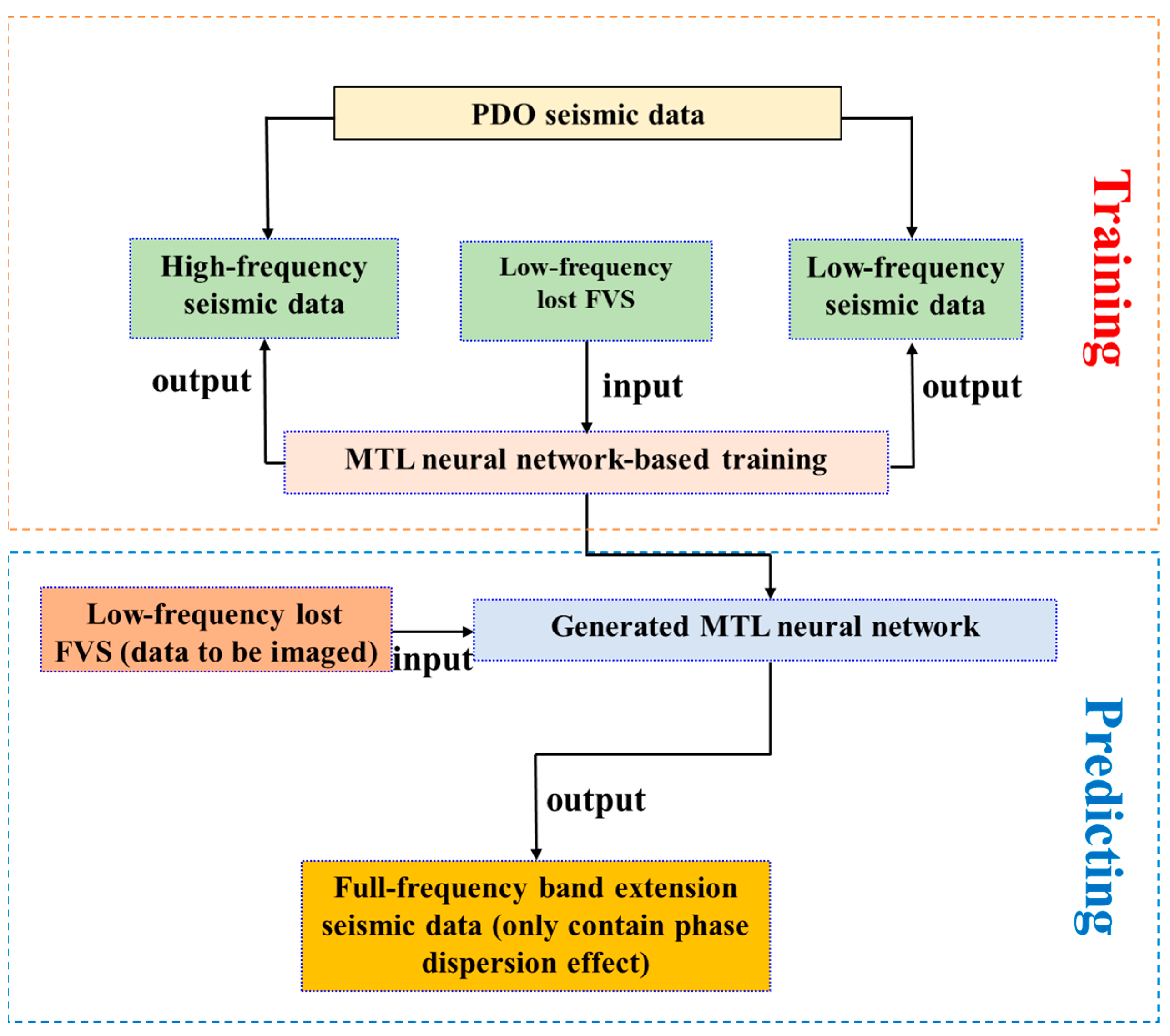
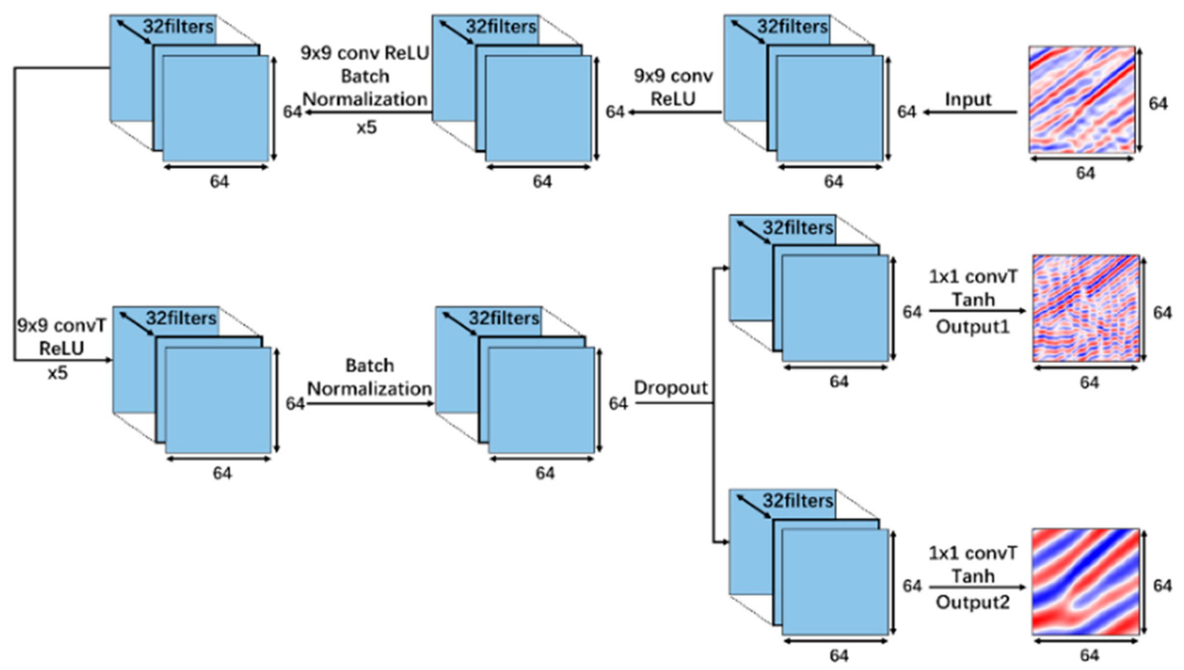
2.2. Network Architecture of Frequency Extension Based on MTL

In Q-RTM, seismic records exhibit both amplitude attenuation and phase dispersion effects. Our method’s primary objective is to eliminate the amplitude attenuation effect from the seismic record data, thereby preventing instability in traditional Q-RTM. To facilitate understanding, we simplify seismic data with amplitude attenuation only as AAO and phase dispersion only as PDO. Additionally, we refer to viscoacoustic seismic data as FVS. The detailed process of expanding seismic data’s full frequency band, based on multi-task learning (MTL), is illustrated in Figure 1. During MTL neural-network-based training, Equation (3) is employed to derive AAO seismic data as the output. Subsequently, we use a bandpass filtering method to generate two types of simulated seismic data: the low-frequency band (typically absent in seismic data) and the high-frequency band (which is attenuated due to the Q effect) seismic data. For input data, Equation (4) is utilized to obtain viscoacoustic seismic data, which incorporates both amplitude attenuation and phase dispersion, while also lacking low-frequency signals. Using these input–output training samples, we train the MTL neural network for full-band frequency extension, establishing a mapping relationship for seismic data. This trained MTL neural network is then employed to predict the missing low-frequency seismic data and high-frequency seismic data affected by the Q effects. Through compensation of the amplitude attenuation effect within the data domain, our approach mitigates the instability typically encountered in traditional Q-RTM.

Figure 2 illustrates the seismic data extension method employing the hard parameter sharing mode within multi-task learning (MTL). In this method, the low-frequency missing FVS seismic data serve as the input domain, while simulated seismic data in both high and low-frequency bands constitute the task domain. Notably, all hidden layers are shared between the input and task domains, enabling the concurrent prediction of high-frequency and low-frequency components when inputting the low-frequency missing FVS seismic data.

The general problem of MTL is expressed as follows: for an independent and identically distributed dataset, such that  ${\{x_i,y_i^1,\dots ,y_i^T\}}_{i\in [N]}$,

$$f^t(x;{\theta }^{share},{\theta }^t):\mathcal{X}\to {\mathcal{Y}}^t,$$

(5)

where T represents the number of tasks, N represents the total number of points in the dataset,  $x_i$ stands for the ith input point in the input space  $\mathcal{X}$, $y_i^t$ represents the ith output point of the task  $t$ in the task space  ${\left\{y^t\right\}}_{t\in [T]}$, and  ${\theta }^t$ and  ${\theta }^{share}$ are the model parameters of the task  $t$ and the model parameters shared with other tasks, respectively. In this study, the mapping from input space to task space can be realized by MTL.

In MTL, multiple tasks are involved in a learning process, and each task has its own learning objective. Considering that different tasks may conflict and need to be weighed, the MTL can be regarded as a multi-objective optimization problem. The objective function  $E{r}_{\min }$ of MTL can be formulated as the empirical risk minimization formula as follows:

$$E{r}_{\min }=\underset{{\theta }^{sh},{\theta }^1,\dots ,{\theta }^T}{{\displaystyle \min }}{\displaystyle \sum _{t=1}^T{c}^t}\frac{1}{N}{\displaystyle {\sum }_iℒ(f^t({\mathrm{x}}_i;{\theta }^{share},{\theta }^t),y_i^t)},$$

(6)

where  $c^t$ denotes the weight of the task  $t$, and the loss function  ${\widehat{ℒ}}^{ \mathrm{t}}$ of the task  $t$ is

$${\widehat{ℒ}}^{ \mathrm{t}}({\theta }^{share},{\theta }^t)\triangleq \frac{1}{N}{\displaystyle {\sum }_iℒ(f^t({\mathrm{x}}_i;{\theta }^{share},{\theta }^t),y_i^t)}.$$

(7)

In the diagram of band expansion based on the hard sharing mode of MTL shown in Figure 2, there are two tasks sharing all hidden layers, and all the tasks are competitive, which means that there are two sets of neural network parameters,  $\theta$ and  $\overline{\theta }$, which have the following relationship:

$$\{\begin{array}{l}{\widehat{ℒ}}^{{ \mathrm{t}}_1}({\theta }^{share},{\theta }^{t_1})<{\widehat{ℒ}}^{{ \mathrm{t}}_1}({\overline{\theta }}^{share},{\overline{\theta }}^{t_1})\\ {\widehat{ℒ}}^{{ \mathrm{t}}_2}({\theta }^{share},{\theta }^{t_2})>{\widehat{ℒ}}^{{ \mathrm{t}}_2}({\overline{\theta }}^{share},{\overline{\theta }}^{t_2})\end{array}.$$

(8)

As shown in Equation (8), if task 2 dominates the training process, task 1 will not be fully learned, and underfitting may occur, reducing the generalization ability of MTL. The above task imbalance phenomenon is common in MTL and significantly affects the performance of MTL models. Therefore, reducing the competition between task 1 and task 2 and alleviating task imbalance is beneficial to the generalization of MTL. In this paper, the task balance factor in MTL is defined as follows:

$$T{b}_{MTL}=\frac{1}{N}{\displaystyle {\displaystyle {\sum }_i}(ℒ(f^t({\mathrm{x}}_i;{\theta }^{share},{\theta }^t),y_i^t)-ℒ(f_0{}^t({\mathrm{x}}_i,{\theta }^t),y_i^t))},$$

(9)

where  $f^t({\mathrm{x}}_i;{\theta }^{share},{\theta }^t)$ and  $f_0{}^t({\mathrm{x}}_i,{\theta }^t)$ are the predicted values at the ith point for task t in MTL and single-task learning, respectively. When the task balance factor  $T{b}_{MTL}>0$, there is task imbalance in MTL. Considering that there is task competition in the MTL framework shown in Figure 2, this paper adds the task balance factor constraint to the traditional MTL objective function:

$$\{\begin{array}{l}\underset{{\theta }^{sh},{\theta }^1,\dots ,{\theta }^T}{{\displaystyle \min }}{\displaystyle \sum _{t=1}^T{c}^t}\frac{1}{N}{\displaystyle {\sum }_iℒ(f^t({\mathrm{x}}_i;{\theta }^{share},{\theta }^t),y_i^t)}\\ T{b}_{MTL}\le 0\end{array}.$$

(10)

Equation (10) turns the learning process of the multi-task model into a constrained optimization problem, so as to alleviate the task imbalance phenomenon and improve the generalization ability of MTL.

The detailed architecture of the neural network designed in this paper is shown in Figure 3. It consists of 1 input layer, 13 convolutional layers, 2 activation functions (ReLU and Tanh), and 2 output layers. The input data element size is  $64\times 64$. In the hidden layer, 32 convolution kernels of fixed size are set for each convolutional layer to capture features, and the hidden layer parameters are shared by the two tasks. The  $9\times 9$ ReLU activation function is used for all layers except the output layer, and the output layer uses the Tanh activation function to fit the data to the [−1, 1] range. In order to accelerate convergence, a batch normalization layer is inserted between several convolutional layers.

2.3. Data Preparation

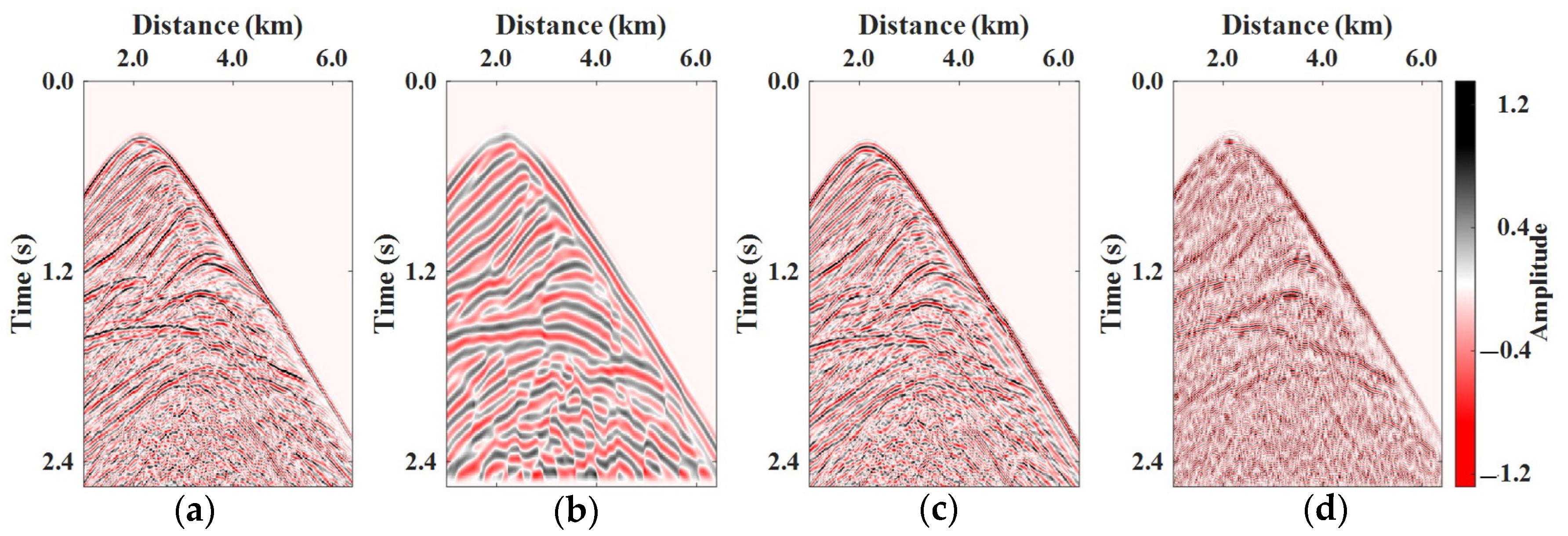
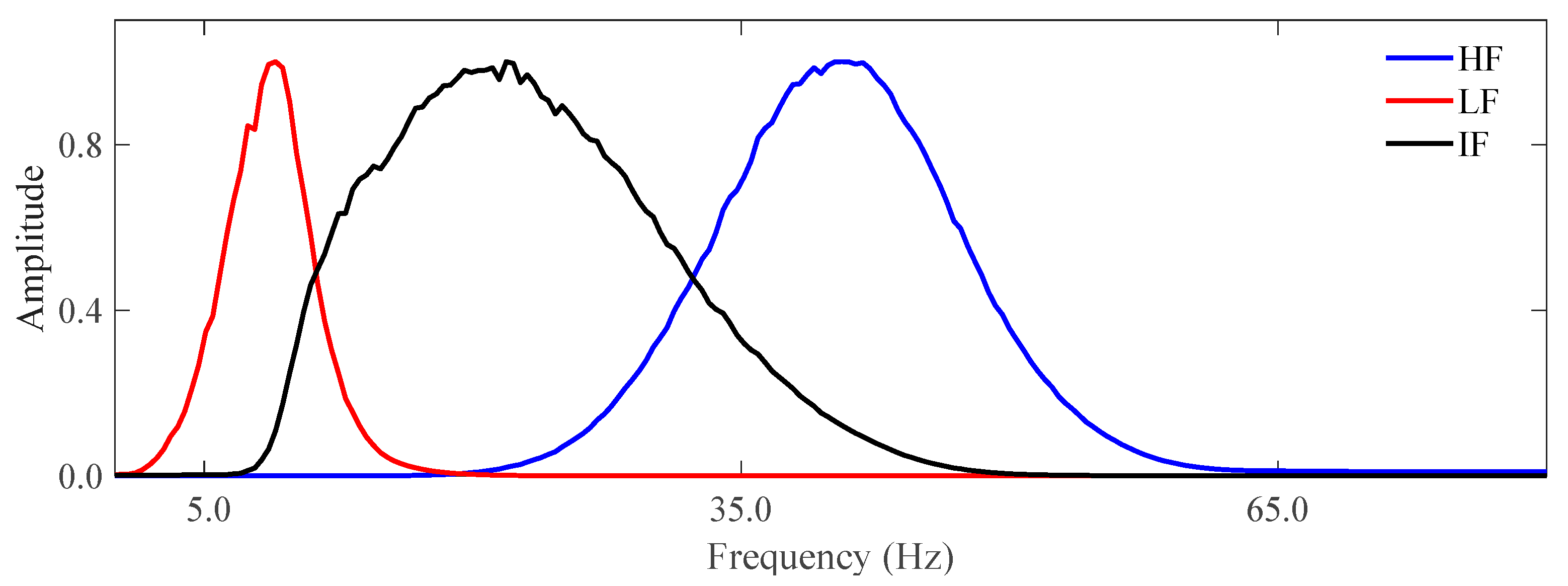
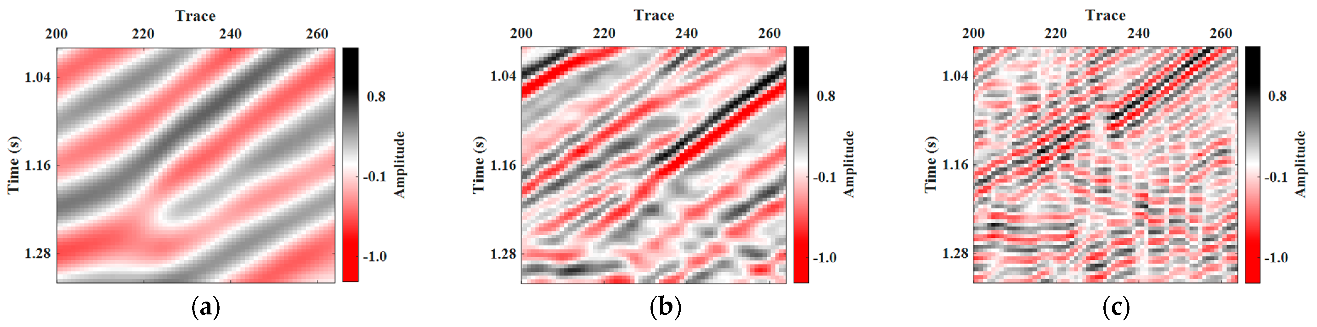
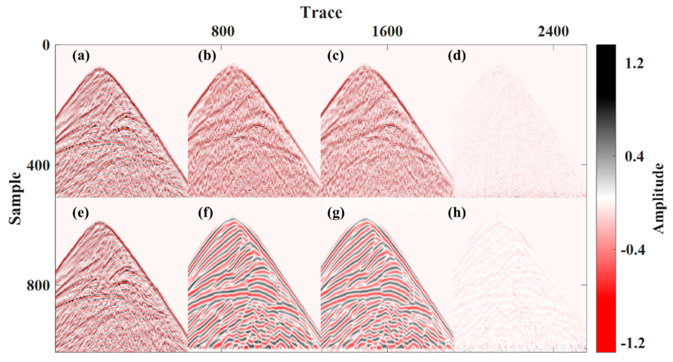
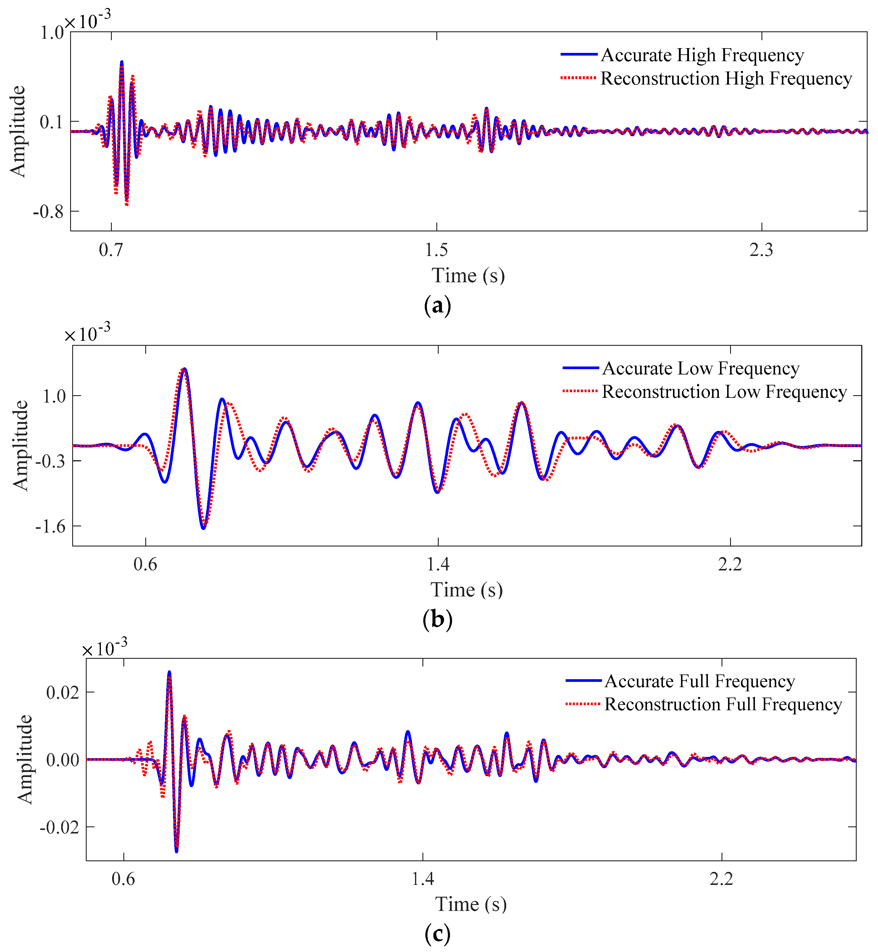
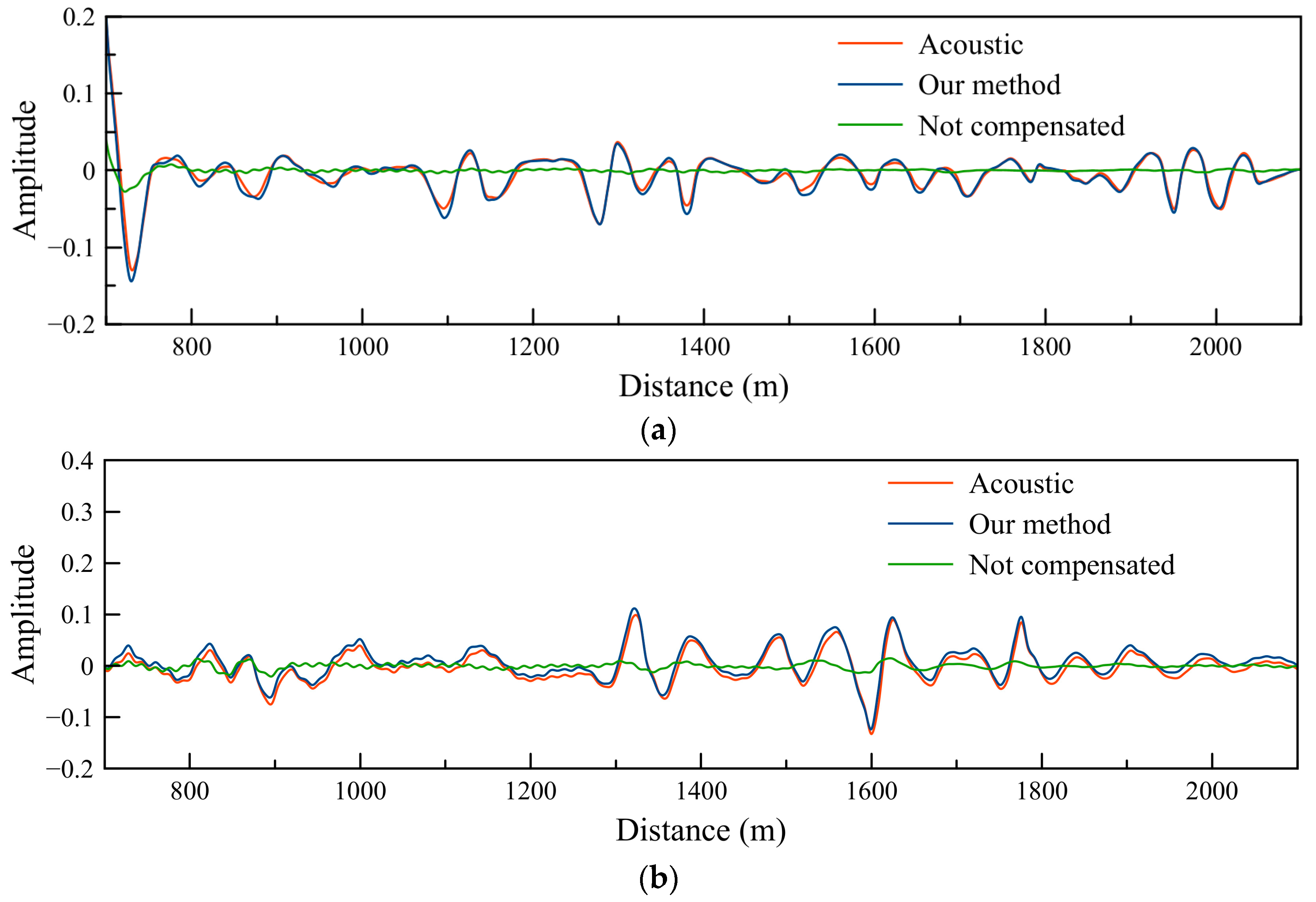
To alleviate the complexities of multi-task learning (MTL) training, it is essential to standardize the amplitude values within seismic records, ensuring uniformity and mitigating data disparities. To safeguard against the direct wave, which possesses substantial energy and could obscure reflected wave information during training, it is imperative to remove the direct wave as a preliminary step. Notably, seismic records exhibit significant amplitude variations, and even after direct wave removal, the energy in the refracted wave surpasses that in the reflected wave. In such scenarios, directly inputting normalized seismic data into the network diminishes the contribution of the reflected wave to network training, thereby compromising network performance and the quality of final imaging results. Consequently, this study employs automatic gain control (AGC) to harmonize amplitude levels [35]:

$$\overline{d}(x,t)=\frac{d(x,t)}{\left[\frac{1}{(2L+1)(2K+1)}{\displaystyle \sum _{l=-L}^L{\displaystyle \sum _{k=-K}^K\left|d(x+l,t+k)\right|}}\right]},$$

(11)

where  $d(x,t)$ and  $\overline{d}(x,t)$ are the first sampling point in the seismic record of the input and output AGC algorithm, respectively, and  $2L+1$ and  $2K+1$ are the horizontal and vertical side lengths of the calculation window, respectively. In the preprocessing stage, seismic records do not need to be normalized, because a batch normalization processing layer is inserted into the network architecture designed in this paper.

In order to simulate the band-limited characteristics of actual seismic data, we use the Butterworth bandpass filtering algorithm for the PDO seismic records obtained by forward modeling:

$$B_N^2(\omega )=1{\displaystyle /}\left(1+{\left(\frac{\omega }{{\omega }_0}\right)}^{2N}\right),$$

(12)

where N is the order of the filter and  ${\omega }_0$ is the cutoff frequency. Then, we can obtain the low-frequency band (typically absent in seismic data) and the high-frequency band seismic data (attenuated due to the Q effect), which are used to make the output dataset for training the MTL.

After the frequency division of the seismic record is completed, data block random matching is also needed. The input and output seismic datasets are divided into several small blocks by the slider method, and the small blocks can be regarded as the basic elements of the gun record. The generalization ability of the network can be improved by using the small blocks of seismic data as the input. The input and output data blocks are randomly combined for the training and testing of the MTL.

3. Examples

In this section, we use a part of the seismic data from the Marmousi model to verify the effectiveness of the proposed method. Figure 4a,b show the velocity and Q model, respectively. In order to save computing power, the number of discrete grids of the actual Marmousi longitudinal wave velocity model is 640 × 230, and the spatial sampling interval is 10 m × 10 m. The velocity ranges from 1500 m/s to 5500 m/s, and Q is determined from velocity in km/s by using the following empirical relation:

$$Q=3.516v^{2.2}.$$

(13)

The value of the Q model shown in Figure 4b ranges from 34.2 to 595.6. The observation system was placed on the surface, and the Ricker wavelet with the dominant frequency of 20 Hz was selected as the source wavelet. The observation system was excited 40 times with 640 receiving channels each time, and the channel spacing was 10 m.

The seismic records are obtained by solving Equation (3), which only contains the phase dispersion effect. Then, they are preprocessed according to the steps described in Section 2. First, we remove the direct wave from the simulated seismic data shown in Figure 5a. Then, we divide the seismic data into two components: low frequency (<10 Hz, shown in Figure 5b) and high frequency (45~80 Hz, shown in Figure 5d), which will be used as the output data in the MTL neural network. The input data for the MTL neural network shown in Figure 5c are obtained by solving Equation (1). All the seismic data shown in Figure 5 were plotted after the implementation of the AGC algorithm.

The average amplitude spectra of the three components are shown in Figure 6. The red and blue lines correspond to Figure 5b,d, respectively, and are used as the two outputs of the MTL. The black line represents the average amplitude spectrum of Figure 5c, which is used as the input of the MTL.

After frequency division, the seismic data are subjected to energy balancing processing, and discrete grids of seismic data blocks with a size of 64 × 64 are obtained through sliders, as shown in Figure 7. These are randomly combined to create middle-frequency, low-frequency, and high-frequency (attenuated because of the Q effect) training or testing datasets, as shown in Figure 8.

In this example, 20 shots of seismic data are randomly selected from the simulated 40 shots of seismic records for the training phase of MTL, and the test of MTL is carried out on the seismic records of the remaining 20 shots of seismic data. Firstly, the training of MTL is performed. After training, the intermediate frequency dataset used for predicting is input into the trained model. The predicted results are shown in Figure 9. From Figure 9d,h, we can see that the residual errors between the real and predicted low- and high-frequency seismic data components are within a reasonable range, and the prediction effect reaches the expected goal.

In order to further verify the effectiveness of our proposed method, the normalized prediction result was restored to the energy level of the original seismic record, and the single seismic record was extracted for comparison. Figure 10a–c represent the high-frequency, low-frequency, and full frequency band components, respectively. The red and blue lines represent the reconstructed and real parts. From Figure 10a, we can notice that the attenuated high-frequency component has a good prediction effect. Although the low-frequency components shown in Figure 10b have some phase errors, the amplitudes are in good agreement. The recovered full-band seismic record shown in Figure 10c is in good agreement with the true full-band frequency seismic record.

After we compensate for the amplitude attenuation according to the aforementioned MTL neural network, we just need to correct the phase dispersion effect by solving Equation (3) in both forward and backward wave propagation. Thus, the instability will be avoided during Q-RTM.

Figure 11 shows the final migration images, including the reference acoustic RTM image for the acoustic data shown in Figure 11a. Figure 11b,c represent the acoustic RTM image for viscoacoustic data and Q-RTM image for viscoacoustic data, respectively. In Figure 11b, the energy attenuation and phase shift lead to a low resolution due to the Q effect, especially for the deeper layers. However, the compensated image obtained by our proposed method has a high resolution in both shadow and deep layers and is very close to the reference one (Figure 11a). Above all, the process of Q-RTM using Equation (3) is absolutely stable.

Figure 12 shows the traces extracted from Figure 11 at the horizon positions of x = 1500 m and 2000 m. The red line is from Figure 11a, the blue and green lines are from the images of our proposed compensated Q-RTM and non-compensated RTM, respectively. It can be seen that the blue line (our method) can match the red line (RTM result of acoustic data) perfectly. This means that the amplitude attenuation and phase dispersion are recovered successfully and that our method is reasonable and feasible.

4. Discussion

In this paper, we present a framework of Q-RTM based on an MTL neural network. The above sections have proved the feasibility of our method. However, we still need to discuss two questions.

The first question is about the training samples. The input and output training samples all only contain the phase dispersion effect, instead of using the acoustic data. This is because the phase dispersion effect controls the travel time of the seismic wave propagation, which is important to seismic imaging, while the amplitude attenuation effect only affects the frequency band. The MTL frequency-extension method is more feasible.

The second question pertains to whether the method presented in this paper can be applied to large-scale real seismic data processing. There is a concern about the computational intensity involved in simulating seismic data and training the network, given the substantial volume of actual seismic data. The following question arises: Is the cost of addressing the instability in Q-RTM too high? However, this concern is largely unwarranted. The underground structures in the actual target areas often exhibit significant similarity. As a result, there is no need for extensive network training; we can focus on training the network for the specific target area. Moreover, we can restore the crucial low-frequency components essential for seismic imaging and inversion. Therefore, the method proposed in this paper is highly worthwhile.

5. Conclusions

In this paper, we introduce a novel approach for addressing instability within the context of the variable fractional Laplacian viscoacoustic wave equation in Q-RTM. Our method focuses on compensating amplitude attenuation in seismic records through the utilization of a multi-task learning (MTL) neural network, rather than altering the wave propagation process. To begin, we train an MTL neural network with input training samples generated by solving the conventional viscoacoustic wave equation (designated as Equation (1)). These samples encompass both amplitude attenuation and phase dispersion effects. We then perform filtering to isolate the low-frequency component, a crucial step due to the absence of this component in real seismic data. The output training samples consist of two tasks: the low-frequency and high-frequency components. These components are derived by filtering the phase-dispersion-only seismic data, which is obtained through the resolution of Equation (3).

Based on the trained MTL neural network, we can stabilize the compensatory amplitude attenuation effect. The migration results of synthetic data show that the compensation results are nearly the same as those without attenuation and dispersion, illustrating that our method is reasonable and feasible.

References

1. Aki, K.; Richards, P. Quantitative Seismology, 2nd ed.; University Science Books: Melville, NY, USA, 1980. [Google Scholar]
2. Wang, Y. A stable and efficient approach of inverse q filtering. Geophysics 2002, 67, 657–663. [Google Scholar] [CrossRef]
3. Wang, Y. Inverse q-filter for seismic resolution enhancement. Geophysics 2006, 71, V51–V60. [Google Scholar] [CrossRef]
4. Li, G.; Liu, Y.; Zheng, H.; Huang, W. Absorption decomposition and compensation via a two-step scheme. Geophysics 2015, 80, V145–V155. [Google Scholar] [CrossRef]
5. Etgen, J.; Gray, S.H.; Zhang, Y. An overview of depth imaging in exploration Geophysics. Geophysics 2009, 74, WCA5–WCA17. [Google Scholar] [CrossRef]
6. Deng, F.; McMechan, G.A. True-amplitude prestack depth migration. Geophysics 2007, 72, S155–S166. [Google Scholar] [CrossRef]
7. Deng, F. Viscoelastic true-amplitude prestack reverse-time depth migration. Geophysics 2008, 73, S143–S155. [Google Scholar] [CrossRef]
8. Zhu, T.; Harris, J.M. Modeling acoustic wave propagation in heterogeneous attenuating media using decoupled fractional laplacians. Geophysics 2014, 79, T105–T116. [Google Scholar] [CrossRef]
9. Zhu, T.; Harris, J.M.; Biondi, B. Q-compensated reverse-time migration. Geophysics 2014, 79, S77–S87. [Google Scholar] [CrossRef]
10. Zhang, Y.; Zhang, P.; Zhang, H. Compensating for visco-acoustic effects in reverse time migration. In Seg Technical Program Expanded Abstracts; Society of Exploration Geophysicists: Houston, TX, USA, 2010; pp. 3160–3164. [Google Scholar]
11. Li, Q.; Zhou, H.; Zhang, Q.; Chen, H.; Sheng, S. Efficient reverse time migration based on fractional laplacian viscoacoustic wave equation. Geophys. J. Int. 2016, 204, 488–504. [Google Scholar] [CrossRef]
12. Chen, H.; Zhou, H.; Qu, S. Lowrank approximation for time domain viscoacoustic wave equation with spatially varying order fractional laplacians. In Proceedings of the 2014 SEG Annual Meeting, Denver, CO, USA, 26–31 October 2014; pp. 3400–3405. [Google Scholar]
13. Sun, J.; Zhu, T. Stable attenuation compensation in reverse-time migration. In Seg Technical Program Expanded; Society of Exploration Geophysicists: Houston, TX, USA, 2015; pp. 3942–3947. [Google Scholar]
14. Yan, H.; Liu, Y. Viscoacoustic prestack reverse-time migration based on the time-space domain adaptive high-order finite-difference method. Geophys. Prospect. 2013, 61, 941–954. [Google Scholar] [CrossRef]
15. Yang, J.; Huang, J.; Zhu, H.; Li, Z.; Dai, N. Viscoacoustic reverse time migration with a robust space-wavenumber domain attenuation compensation operator. Geophysics 2021, 86, S339–S353. [Google Scholar] [CrossRef]
16. Aghamiry, H.S.; Gholami, A. Interval-Q estimation and compensation: An adaptive dictionary-learning approach. Geophysics 2018, 83, V233–V242. [Google Scholar] [CrossRef]
17. Shao, J.; Wang, Y. Simultaneous inversion of Q and reflectivity using dictionary learning. Geophysics 2021, 86, R763–R776. [Google Scholar] [CrossRef]
18. Sun, H.; Demanet, L. Low-frequency extrapolation with deep learning. In SEG Technical Program Expanded Abstracts; Society of Exploration Geophysicists: Houston, TX, USA, 2018; pp. 2011–2015. [Google Scholar]
19. Fang, J.; Zhou, H.; Elita Li, Y.; Zhang, Q.; Wang, L.; Sun, P.; Zhang, J. Data-driven low-frequency signal recovery using deep-learning predictions in full-waveform inversion. Geophysics 2020, 85, A37–A43. [Google Scholar] [CrossRef]
20. Hu, W.; Jin, Y.; Wu, X.; Chen, J. Progressive transfer learning for low-frequency data prediction in full-waveform inversion. Geophysics 2021, 86, R369–R382. [Google Scholar] [CrossRef]
21. Ovcharenko, O.; Kazei, V.; Kalita, M.; Peter, D.; Alkhalifah, T. Deep learning for low-frequency extrapolation from multioffset seismic data. Geophysics 2019, 84, R989–R1001. [Google Scholar] [CrossRef]
22. Ovcharenko, O.; Kazei, V.; Plotnitskiy, P.; Peter, D.; Silvestrov, I.; Bakulin, A.; Alkhalifah, T. Extrapolating low-frequency prestack land data with deep learning. In Proceedings of the SEG International Exposition and Annual Meeting, Virtual, 11–16 October 2020; pp. 1546–1550. [Google Scholar]
23. Ovcharenko, O.; Kazei, V.; Alkhalifah, T.A.; Peter, D.B. Multi-task learning for low-frequency extrapolation and elastic model building from seismic data. IEEE Trans. Geosci. Remote Sens. 2022, 60, 1–17. [Google Scholar] [CrossRef]
24. Duong, L.; Cohn, T.; Bird, S.; Cook, P. Low resource dependency parsing: Cross-lingual parameter sharing in a neural network parser. In Proceedings of the 53rd Annual Meeting of the Association for Computational Linguistics and the 7th International Joint Conference on Natural Language Processing (Short Papers), Beijing, China, 26–31 July 2015; pp. 845–850. [Google Scholar]
25. Yang, Y.; Hospedales, T.M. Trace norm regularised deep multi-task learning. arXiv 2016, arXiv:1606.04038. [Google Scholar]
26. Caruana, R. Multitask learning: A knowledge-based source of inductive bias. In Proceedings of the Tenth International Conference on Machine Learning, San Francisco, CA, USA, 27–29 July 1993; pp. 27–29. [Google Scholar]
27. Long, M.; Cao, Z.; Wang, J.; Yu, P.S. Learning multiple tasks with multilinear relationship networks. Adv. Neural Inf. Process. Syst. 2017, 30. [Google Scholar]
28. Bruggemann, D.; Kanakis, M.; Georgoulis, S.; Van Gool, L. Automated search for resource-efficient branched multi-task networks. arXiv 2020, arXiv:2008.10292. [Google Scholar]
29. Liu, P.; Qiu, X.; Huang, X. Adversarial multi-task learning for text classification. arXiv 2017, arXiv:1704.05742. [Google Scholar]
30. Zhao, X.; Li, H.; Shen, X.; Liang, X.; Wu, Y. A modulation module for multi-task learning with applications in image retrieval. In Proceedings of the European Conference on Computer Vision, Munich, Germany, 8–14 September 2018; pp. 401–416. [Google Scholar]
31. Chen, Z.; Badrinarayanan, V.; Lee, C.Y.; Rabinovich, A. Gradnorm: Gradient normalization for adaptive loss balancing in deep multitask networks. In Proceedings of the 35th International Conference on Machine Learning, Stockholm, Sweden, 10–15 July 2018; pp. 794–803. [Google Scholar]
32. Lin, X.; Zhen, H.L.; Li, Z.; Zhang, Q.F.; Kwong, S. Pareto multi-task learning. Adv. Neural Inf. Process. Syst. 2019, 32. [Google Scholar]
33. Sener, O.; Koltun, V. Multi-task learning as multi-objective optimization. Adv. Neural Inf. Process. Syst. 2018, 31. [Google Scholar]
34. Versteeg, R. The Marmousi experience: Velocity model determination on a synthetic complex data set. Lead. Edge 1994, 13, 927–936. [Google Scholar] [CrossRef]
35. Rajagopalan, S.; Milligan, P. Image Enhancement of Aeromagnetic Data using Automatic Gain Control, Exploration. Geophysics 1994, 25, 173–178. [Google Scholar]
Figure 1. Full-band extension of MTL based on simulated data.
Fractalfract 07 00874 g001
Figure 2. Schematic diagram of seismic data band expansion in hard parameter sharing mode.
Fractalfract 07 00874 g002
Figure 3. Detailed architecture of our MTL-based frequency-extension framework.
Fractalfract 07 00874 g003
Figure 4. The modified Marmousi (a) velocity and (b) Q model.
Fractalfract 07 00874 g004
Figure 5. The 14th (a) phase-dispersion-only seismic data obtained using Equation (3) and their (b) filtered low-frequency component and (d) filtered high-frequency component. (d) The viscoacoustic seismic data obtained using Equation (1) with the low-frequency component cut off. Note that all the figures show data plotted after the implementation of the AGC algorithm.
Fractalfract 07 00874 g005
Figure 6. The average amplitude spectra of seismic data shown in Figure 5. The red and black lines correspond to Figure 5b,c, respectively. The blue line represents the average amplitude spectrum of Figure 5d.
Fractalfract 07 00874 g006
Figure 7. Data patch acquisition method diagram.
Fractalfract 07 00874 g007
Figure 8. The combination of low-frequency (a), medium-frequency (b), and high-frequency (attenuated because of the Q effect) (c) data patches.
Fractalfract 07 00874 g008
Figure 9. Comparison of prediction results from our MTL neural network. The upper and lower parts stand for the high-frequency and low-frequency seismic data. From left to right are the simulated PDO seismic data, real low- or high-frequency seismic data, predicted low- or high-frequency seismic data, and residual errors between the real and predicted seismic data.
Fractalfract 07 00874 g009
Figure 10. Comparison of (a) the high-frequency, (b) low-frequency, and (c) full frequency band single traces. The red and blue lines represent the reconstructed and real parts.
Fractalfract 07 00874 g010
Figure 11. (a) Acoustic RTM image of acoustic data, reference imaging; (b) acoustic RTM image of viscoacoustic data, without Q compensation; and (c) Q-RTM image of viscoacoustic data, our proposed method.
Fractalfract 07 00874 g011
Figure 12. Waveform plot of traces located at (a x = 1500  m and (b x = 2000  m. The red line is from the acoustic RTM image for acoustic data, the blue and green lines are from the images of our proposed compensated Q-RTM and non-compensated RTM, respectively.
Fractalfract 07 00874 g012
Disclaimer/Publisher’s Note: The statements, opinions and data contained in all publications are solely those of the individual author(s) and contributor(s) and not of MDPI and/or the editor(s). MDPI and/or the editor(s) disclaim responsibility for any injury to people or property resulting from any ideas, methods, instructions or products referred to in the content.