Adaptive Backstepping Boundary Control for a Class of Modified Burgers’ Equation

Abstract

Burgers’ equation is used to describe wave phenomena in hydrodynamics and acoustics. It was derived originally as a prototype to provide analytic insight into the nature of turbulence and its modeling, and has found applications in the study of shock waves and wave transmission. Burgers’ equation is not globally controllable, and under certain conditions it can be neutrally stable. In this study, we explore the adaptive backstepping boundary control (BBC) methodology on a modified Burgers’ equation with unknown parameters, but constant, for the reactive and convective (nonlinear) terms, with Robin and Neumann boundary conditions (BCs), where this latter BC is actuated by the control signal. The nominal controller is designed from a linear partial differential equation (PDE), and under the assumption that this nominal controller also achieves stabilization for the modified Burgers’ equation, then its adaptive version is proposed for the control of such nonlinear PDE systems. Simulation results show convergence near the ideal values for the parametric estimates while the estimation error converges to zero.

1. Introduction

Partial differential equations (PDEs) are employed to describe the behavior from heat transfer, fluid flows, electrostatic fields, vibrations or wave phenomena [1] and also have been objects of study in novel areas concerned with traffic flow control, gas and oil extraction, neural networks, machine learning, neuroscience, information science and quantum systems [2,3,4,5]. Moreover, the modeling of soft robots by means of PDEs to the design of feedback controllers is still an open research topic [6]. In accordance with its properties, the PDEs are classified into parabolic, elliptic and hyperbolic types. Due to the temporal and spatial interaction between their parameters and variables, such PDEs systems are also referred as distributed parameter systems (DPSs). A PDE in a domain together with a set of initial and/or boundary conditions (BCs) that retains the existence, uniqueness, and stability properties is said to be a well-posed problem [7].

Burgers’ equation is used to describe wave phenomena in hydrodynamics and acoustics. Burgers was interested in the equation as a one-dimensional model of viscous compressible flow. It was derived originally as a prototype to provide analytic insight into the nature of turbulence and its modeling, and has found applications in the study of shock waves and wave transmission. Also, it is considered analogous to the Navier–Stokes equation. Moreover, it has been shown that Burgers’ equation with an external forcing term can be reduced to an one-dimensional heat equation plus a potential term via the Hopf–Cole transformation. It should be noted that in the case of radiation or Neumann BCs, this latter transformation is not of great help since these conditions are transformed into quadratically nonlinear conditions. So, this fact does not allow us to treat the above mentioned linear heat equation by standard methods. Besides, the Burgers’ equation can be linked with the linear heat equation via Bäcklund transformation. Furthermore, it is well-known that the uncontrolled problem for the Burgers’ equation with homogeneous Neumann BCs is not asymptotically stable. Additionally, Burgers’ equation is not globally controllable, and under certain conditions it can be neutrally stable [8,9,10,11,12,13].

Generally, finding exact solutions for nonlinear PDEs and the practical problem may be hard. Due to such a reason, many numerical methods are frequently applied to achieve this goal [14,15,16,17]. The solution of the general Burgers equation is quite complex, and few researchers study the theoretical solution of this equation. Instead, many other researchers have considered various numerical discretization methods to solve it. In [14], a robust implicit difference scheme was proposed in order to compensate the singular behavior of the exact solution at the initial time introducing graded meshes. The Galerkin method, based on piece-wise linear test functions, was used to handle the nonlinear convection term, whereas the Taylor expansion, with an integral remainder, was used to deal with fourth- and second-order terms. Existence, stability, convergence and uniqueness properties of the numerical solutions were proved. Also, two nonlinear iterative methods, namely the linearized iterative algorithm and the Newton iterative method, were introduced to solve the nonlinear system. Most of the existing approximate methods for solving fourth-order partial integro-differential equations (PIDEs) with a weakly singular kernel (WSK) are unbalanced, i.e., a low order scheme, such as finite difference methods; for integrating the temporal variable and a high-order numerical structure, such as the spectral-like method, the discretization of space variables are used. The Sinc-collocation method is an effective technique against the singularities of the equations. In [15], a fully space–time Sinc-collocation method was developed for a fourth-order heat model arising in viscoelasticity, which is a family of fourth-order PIDEs involving weak singularity. The Sinc method for the Volterra integral term was constructed. Exponential convergence simultaneously in space and time for the proposed method was proved. As a general form of PIDEs, the nonlocal evolution equations with a WSK are recognized as an efficient tool to describe the properties of complex dynamical processes more accurately than the integer derivatives and integrals. The application of the nonlocal evolution equations encompasses a wide spectrum of topics. The three-dimensional nonlocal evolution equation with the WSK is in a preliminary stage of development, and its potential remains to be fully explored. In [16], a backward Euler alternating direction implicit (ADI) finite difference method for the three-dimensional nonlocal evolution equation with the WSK was devised, which significantly reduces the computational cost. The ADI method is an effective numerical method for high dimensional PIDEs, which reduce the high dimensional problem to sets of independent one-dimensional problems. Stability and convergence analysis were proven when introducing two new inner products and norms. A first-order fractional convolution quadrature scheme and the backward Euler ADI method were proposed to approximate a Riemann–Liouville fractional integral term and to discretize the temporal derivative, respectively. In [17], an orthogonal spline collocation (OSC) method for approximating a multi-term fourth-order subdiffusion equation with non-smooth solutions was developed. The multi-term fourth-order subdiffusion equation is an effective tool for modeling anomalous phenomena and complex systems in engineering and natural science, having some advantages over integer-order PDEs in describing real processes or phenomena with memory. The graded meshes method to handle the initial weak singularity of the unknown solution at the initial time was employed in the temporal direction, whereas the OSC method was used in the spatial direction.

Under a nonlinear feedback linearizing transformation approach and using the backstepping boundary control (BBC) method for PDEs [18,19], a full state feedback law was designed in order to stabilize shock profiles from the viscous Burgers’ equation actuated at its boundaries. Then, the design of a nonlinear observer, output feedback stabilization and trajectory tracking for the viscous Burgers’ equation were addressed in [20,21,22].

Although not in a direct way, the adaptive control approach for ordinary differential equations (ODEs) from finite dimension has been spread to the control of PDEs of infinite dimension, successfully contributing to the parametric estimation of its ideal parameters. The adaptive control technique has been studied in some classes of DPSs. A review can be found in [10,23]. In [10], the problem of global asymptotic stability, when considering Neumann and Dirichlet boundary control, was solved for the viscous and inviscid Burgers’ equations through the design of nonlinear boundary control laws under the control Lyapunov function approach. In this latter work, the viscosity parameter was considered as uncertain, and the control of their respective stochastic versions was also addressed. Moreover, an observer-based version was developed for the Dirichlet boundary control of the viscous Burgers’ equation for which measurement in the interior of the domain is required, but it may be impossible to obtain [24]. In [23], an adaptive regulator for a viscous Burgers’ equation was designed under a high-gain nonlinear output feedback approach ensuring global asymptotic stability. Also, it was shown that his proposal can be generalized to higher-order nonlinear PDEs systems. In [25], the trajectory tracking problem and disturbance attenuation to the viscous Burgers’ equation was addressed under the geometric regulation theory approach.

In [26,27,28], early studies on estimation error convergence in DPSs were conducted. In such works, the model reference adaptive control (MRAC) approach for PDEs was examined. Designs of robust adaptive controllers for the Burgers’ equation, regarding unknown viscosity, under Lyapunov’s direct method were reported in [10,29]. An adaptive version for a boundary controller of a parabolic PDE, this latter including an unknown parameter that destabilizes the system, was proposed in [30]. In [31,32], under the output feedback approach, adaptive boundary controllers for unstable infinite relative degree parabolic type PDEs were developed. In [33], adaptive controllers for parabolic type PDEs with spatially-varying parameters as well as with actuation in the boundary were introduced. Convergence of the estimation and parametric errors was guaranteed under Lyapunov’s framework. Adaptive boundary controllers designed for unstable parabolic PDEs under the backstepping control framework were reported in [34,35,36]. Moreover, the adaptive control problem for hyperbolic PDEs, namely one-dimensional systems of coupled linear hyperbolic PDEs, relying on the backstepping approach was treated in [4].

Adaptive BBC approach for PDEs has become a useful constructive design method for both state and unknown parameter estimation with control signal actuation in the boundary, offering the advantage of neglecting the placement of actuators and sensors in the domain [37]. In [19], adaptive BBC design schemes for PDEs based on Lyapunov’s method, swapping and passive identifiers, the latter being inspired on the basis of the certainty equivalence principle, were addressed.

The backstepping design method has shown to have great potential in the control of nonlinear PDEs. In some PDEs, the nonlinearity appears in a manner that does not affect the stability; thus, as for the Burgers’ equation in [29,38,39,40], the selection of a Lyapunov function is very simple. In fact, the experience has shown that the addition of viscosity yields smooth solutions for a nonlinear equation, and that the addition of a nonlinearity can stabilize a linear equation.

In our work, we try with the control of a one-dimensional parabolic type modified Burgers’ equation via adaptive BBC methodology under the criteria of parametric uncertainties to the reactive and viscosity terms, BCs of Robin and Neumann, and actuation of the control signal on this latter BC.

This paper is arranged as follows. Function space properties are summarized in Section 2. In Section 3, the design of a BBC for a Reaction–Advection–Diffusion (RAD) equation is shown. The modified Burgers’ system is described in Section 4. The identifier PDE is given in Section 5. In Section 6, the estimation error PDE is given. Section 7 summarizes the design of the parametric update (adaptive) laws. Dynamics from the boundary control are exhibited in Section 8. In Section 9, interpretation of the results and research directions are given. Conclusions are drawn at the end.

2. Function Spaces

Let $\Omega$ be an open set of ${\mathbb{R}}^n$ with boundary $\mathsf{\Gamma }$. Consider that either $\Omega$ is ${\mathcal{C}}^r$, for $r\ge 1$, or $\Omega$ is Lipschitz. Let $x=\{x_1,\dots ,x_n\}$ be the generic point of ${\mathbb{R}}^n$; so, $dx=d{x}_1\dots d{x}_n$ denotes the Lebesgue measure on ${\mathbb{R}}^n$. $\mathcal{C}(\Omega )$ denotes the space of real continuous functions on $\Omega$, $\mathcal{C}\left(\overline{\Omega }\right)$ denotes the space of real continuous functions on $\overline{\Omega }$. ${\mathcal{C}}^k(\Omega ),k\in \mathbb{N}$ or $k=\infty$ denotes the space for functions k times continuously differentiable on $\Omega$, ${\mathcal{C}}^k\left(\overline{\Omega }\right)$ denotes the space for functions k times continuously differentiable on $\Omega$. ${\mathcal{C}}_0^{\infty }$ denotes the spaces of real ${\mathcal{C}}^{\infty }$ functions on $\Omega$ with compact support in $\Omega$.

Let us consider ${\mathcal{L}}_2(\Omega )$ a Hilbert space for the scalar product

$$(u,v)={\int }_{\Omega }u\left(x\right)v\left(x\right)dx$$

(1)

with norm given by

$$\mid u\mid ={\parallel u\parallel }_{{\mathcal{L}}_2(\Omega )}={\left\{(u,u)\right\}}^{1/2}.$$

(2)

The space of bounded and measurable real functions on $\Omega$ is represented by ${\mathcal{L}}_{\infty }(\Omega )$, a Banach space for the norm

$${\parallel u\parallel }_{{\mathcal{L}}_{\infty }(\Omega )}=\mathrm{ess}{\sup }_{x\in \Omega }\left|u\left(x\right)\right|.$$

(3)

The space of real functions on $\Omega$, which are ${\mathcal{L}}_p$ for the Lebesgue measure, is represented by ${\mathcal{L}}_p(\Omega )$, for $p\in [1,\infty )$, a Banach space for the norm

$${\parallel u\parallel }_{{\mathcal{L}}_p(\Omega )}={\left({\int }_{\Omega }{\left|u\left(x\right)\right|}^{p}dx\right)}^{1/p}.$$

(4)

The Sobolev space of functions u in ${\mathcal{L}}_p(\Omega )$ is denoted by ${\mathcal{W}}^{s,p}(\Omega )$, $s\in \mathbb{N},p\in [1,\infty ]$, whose derivatives of order equal to or less than s are in ${\mathcal{L}}_p(\Omega )$, a Banach space for the norm

$${\parallel u\parallel }_{{\mathcal{W}}^{s,p}(\Omega )}=\sum _{\left[\alpha \right]\le s}{\parallel D^{\alpha }u\parallel }_{{\mathcal{L}}_p(\Omega )}$$

(5)

with $D_{i}u=\partial u/\partial x_i$, $i\in [1,n]$, denoting partial differential derivatives of u, $D^{\alpha }u=D_1^{{\alpha }_1}\dots D_n^{{\alpha }_n}u=\left({\partial }^{{\alpha }_1+\cdots +{\alpha }_n}u\right)/(\partial x_1^{{\alpha }_1}\dots \partial x_n^{{\alpha }_n})$, $\left[\alpha \right]={\alpha }_1+\cdots +{\alpha }_n$ and $\alpha =\{{\alpha }_1,\dots ,{\alpha }_n\}\in {\mathbb{N}}^n$.

For the scalar product

$${\left((u,v)\right)}_{{\mathcal{H}}^s(\Omega )}=\sum _{\left[\alpha \right]\le s}(D^{\alpha }u,D^{\alpha }v),$$

(6)

${\mathcal{W}}^{s,2}(\Omega )={\mathcal{H}}^s(\Omega )$ is a Hilbert space.

Consider the Sobolev spaces ${\mathcal{H}}^s(\Omega )$ comprising ${\mathcal{C}}^{\infty }\left(\overline{\Omega }\right)$ and ${\mathcal{C}}^s\left(\overline{\Omega }\right)$. The closure of ${\mathcal{C}}_0^{\infty }(\Omega )$ in ${\mathcal{H}}^s(\Omega )$ is denoted by ${\mathcal{H}}_0^s(\Omega )$. The closure of ${\mathcal{C}}_0^{\infty }(\Omega )$ in ${\mathcal{W}}^{s,p}(\Omega )$ is denoted by ${\mathcal{W}}_0^{s,p}(\Omega )$.

For the scalar product

$${\left((u,v)\right)}_{{\mathcal{H}}^1(\Omega )}=(u,v)+\sum _{i=1}^n(D_{i}u,D_{i}v),$$

(7)

$${\mathcal{H}}^1(\Omega )=\{u\in {\mathcal{L}}_2(\Omega ),D_{i}u\in {\mathcal{L}}_2(\Omega ),1\le i\le n\}$$

(8)

and

$${\mathcal{H}}_0^1(\Omega )=\mathrm{The}\mathrm{closure}\mathrm{of}{\mathcal{C}}_0^{\infty }(\Omega )\mathrm{in}{\mathcal{H}}^1(\Omega )$$

(9)

are Hilbert spaces.

The Poincaré inequality

$$\left|u\right|\le c_0(\Omega ){\left\{\sum _{i=1}^n{\left|D_{i}u\right|}^2\right\}}^{1/2},$$

(10)

for all $u\in {\mathcal{H}}_0^1(\Omega )$, for a bounded $\Omega$, implies that for the scalar product

$$\left((u,v)\right)=\sum _{i=1}^n(D_{i}u,D_{i}v)$$

(11)

with norm given by

$$\parallel u\parallel ={\left\{\left((u,u)\right)\right\}}^{1/2},$$

(12)

${\mathcal{H}}_0^1(\Omega )$ is a Hilbert space equivalent to ${\mathcal{H}}^1(\Omega )$ [41].

3. BBC Design Methodology for PDEs

The BBC design methodology for PDEs consists of introducing a Volterra integral transformation with a integration kernel along with a control law that maps the PDE system into a stable objective system. So, the PDE system is stabilized due to the invertibility of the transformation since the equivalence of norms between both PDE and objective systems holds. In this section, we show the design procedure of a BBC for a RAD equation [42].

In our analysis, all functions are dependant on the spatial variable x and time t. For easy of notation, only those functions for which the argument is highlighted are those for which its BC is particularly referred to $x=0$ or $x=1$.

Consider the RAD system

$$\begin{array}{cc}\hfill u_t& =u_{xx}+b{u}_x+\lambda u,\hfill \end{array}$$

(13)

$$\begin{array}{cc}\hfill u_x\left(0\right)& =-\frac{b}{2}u\left(0\right),\hfill \end{array}$$

(14)

$$\begin{array}{cc}\hfill u_x\left(1\right)& =\mathcal{U}\left(t\right),\hfill \end{array}$$

(15)

with u a function with domain $x\in [0,1]$ and $t\in [0,\infty )$ in the spatial variable and time, respectively, with b, $\lambda$ as constant parameters, Neumann BCs and actuation (Neumann actuation) signal $\mathcal{U}\left(t\right)$, diffusion term $u_{xx}$, advection term $b{u}_x$ and reaction term $\lambda u$. Let us define

$$\begin{array}{cc}\hfill v& =e^{(b/2)x}u\hfill \end{array}$$

(16)

as a change of variables. From (16), the temporal derivative results

$$\begin{array}{cc}\hfill u_t& =e^{-(b/2)x}{v}_t\hfill \end{array}$$

(17)

while its spatial derivatives as

$$\begin{array}{cc}\hfill u_x& =e^{-(b/2)x}{v}_x-\frac{b}{2}{e}^{-(b/2)x}v\hfill \end{array}$$

(18)

and

$$\begin{array}{cc}\hfill u_{xx}& =e^{-(b/2)x}{v}_{xx}-b{e}^{-(b/2)x}{v}_x+\frac{b^2}{4}{e}^{-(b/2)x}v.\hfill \end{array}$$

(19)

So, under the change of variables (16), the term $u_x$ is removed from the linear PDE (13) which becomes

$$\begin{array}{cc}\hfill v_t& =v_{xx}+{\lambda }_{0}v\hfill \end{array}$$

(20)

with ${\lambda }_0=\lambda -\frac{b^2}{4}$. The BCs are inferred by deriving (16), i.e.,

$$\begin{array}{cc}\hfill v_x& =e^{(b/2)x}{u}_x+\frac{b}{2}{e}^{(b/2)x}u,\hfill \end{array}$$

(21)

which, for $x=0$ results

$$\begin{array}{cc}\hfill v_x\left(0\right)& =u_x\left(0\right)+\frac{b}{2}u\left(0\right).\hfill \end{array}$$

Thus, from (14),

$$\begin{array}{cc}\hfill v_x\left(0\right)& =0.\hfill \end{array}$$

(22)

Now, evaluating (21) for $x=1$ results

$$\begin{array}{cc}\hfill v_x\left(1\right)& =e^{b/2}{u}_x\left(1\right)+\frac{b}{2}{e}^{b/2}u\left(1\right).\hfill \end{array}$$

(23)

Later, Equation (20) has the form of a Reaction–Diffusion (RD) equation, i.e., it is a reduced model from (13), with BCs (22)–(23).

3.1. Stable Objective System

The desirable behavior to be performed by (20) should be defined through a stable objective system. So, let us take the heat equation

$$\begin{array}{cc}\hfill w_t& =w_{xx},\hfill \end{array}$$

(24)

$$\begin{array}{cc}\hfill w_x\left(0\right)& =0,\hfill \end{array}$$

(25)

$$\begin{array}{cc}\hfill w_x\left(1\right)& =-\frac{1}{2}w\left(1\right),\hfill \end{array}$$

(26)

as objective system, with Neumann BCs to the function w with domain $x\in [0,1]$ and $t\in [0,\infty )$. Next, we must demonstrate exponential stability of the system (24)–(26) in the ${\mathcal{L}}_2$-norm, namely,

$$\begin{array}{cc}\hfill \parallel w\parallel & ={\left({\int }_0^1{w}^{2}dx\right)}^{1/2}.\hfill \end{array}$$

(27)

Let us consider the Lyapunov function

$$\begin{array}{cc}\hfill V& =\frac{1}{2}{\int }_0^1{w}^{2}dx\hfill \end{array}$$

(28)

with time derivative

$$\begin{array}{cc}\hfill \dot{V}& ={\int }_0^{1}w{w}_{t}dx\hfill \end{array}$$

(29)

which, from (24), can be written as

$$\begin{array}{cc}\hfill \dot{V}& ={\int }_0^{1}w{w}_{xx}dx.\hfill \end{array}$$

(30)

By applying integration by parts we have

$$\begin{array}{cc}\hfill \dot{V}& =w\left(1\right)w_x\left(1\right)-w\left(0\right)w_x\left(0\right)-{\int }_0^1{w}_x^{2}dx,\hfill \end{array}$$

which, from BCs (25)–(26), is reduced to

$$\begin{array}{cc}\hfill \dot{V}& =-\frac{1}{2}{w}^2\left(1\right)-{\int }_0^1{w}_x^{2}dx.\hfill \end{array}$$

(31)

The linkage between ${\mathcal{L}}_2$-norms of w and $w_x$ is established in the following lemma.

Lemma 1 

(Poincaré Inequality [43]). For any $w\in {\mathcal{H}}^1(0,1)$ (Sobolev space) the following relations hold

$$\begin{array}{c}\hfill \begin{array}{cc}\hfill {\int }_0^1{w}^{2}dx& \le 2w^2\left(1\right)+4{\int }_0^1{w}_x^{2}dx,\hfill \\ \hfill {\int }_0^1{w}^{2}dx& \le 2w^2\left(0\right)+4{\int }_0^1{w}_x^{2}dx.\hfill \end{array}\end{array}$$

(32)

Proof See [43].

So, multiplying (31) by a constant we have

$$\begin{array}{cc}\hfill 4\dot{V}& =-2w^2\left(1\right)-4{\int }_0^1{w}_x^{2}dx.\hfill \end{array}$$

(33)

From Lemma 1, Equation (33) is simplified to

$$\begin{array}{cc}\hfill \dot{V}& \le -\frac{1}{4}{\int }_0^1{w}^{2}dx.\hfill \end{array}$$

(34)

Thus, considering (28), this latter inequality can be rewritten as

$$\begin{array}{cc}\hfill \dot{V}& \le -\frac{1}{2}V.\hfill \end{array}$$

(35)

Solving this last relation by integration we arrive at

$$\begin{array}{cc}\hfill ln\left(V\right)& \le -\frac{1}{2}t+c.\hfill \end{array}$$

(36)

Later, from the property for logarithms

$$\begin{array}{cc}\hfill e^{ln\left(V\right)}& \le e^{-(1/2)t}{e}^c,\hfill \end{array}$$

which is equivalent to

$$\begin{array}{cc}\hfill V& \le e^{-(1/2)t}{e}^c.\hfill \end{array}$$

(37)

Then, evaluating (37) for $t=0$ results

$$\begin{array}{cc}\hfill V(x,0)& \le e^c.\hfill \end{array}$$

(38)

Next, it should be proved that $V\le V(x,0)$. So, from the desirable property

$$\dot{V}\le 0,$$

(39)

integrating and evaluating limits it yields

$$\begin{array}{cc}\hfill V-V(x,0)& \le 0.\hfill \end{array}$$

Then,

$$\begin{array}{cc}\hfill V& \le V(x,0).\hfill \end{array}$$

Also, from (37) and (38),

$$\begin{array}{cc}\hfill V& \le e^{-(1/2)t}V(x,0).\hfill \end{array}$$

(40)

Moreover, from (28) and (27),

$$\begin{array}{cc}\hfill \frac{1}{2}{\int }_0^1{w}^{2}dx& \le \frac{1}{2}{e}^{-(1/2)t}{\int }_0^1{w}^2(x,0)dx.\hfill \end{array}$$

(41)

At last,

$$\begin{array}{cc}\hfill \parallel w\parallel & \le e^{-(1/4)t}\parallel w_0\parallel \hfill \end{array}$$

(42)

where $w_0$ is for $w(x,0)$. In the manner given above, exponential stability of the PDE system (24)–(26) has been proved.

3.2. Backstepping Transformation

Following the BBC methodology for PDEs [18], the coordinate (Volterra integral) transformation

$$\begin{array}{cc}\hfill w& =v-{\int }_0^{x}k(x,y)v\left(y\right)dy\hfill \end{array}$$

(43)

is exploited to convert the reduced model (20), with BCs (22) and (23), into the stable objective system (24)–(26). From the invertibility property of the Volterra integral transformation, the smoothness of the kernel (kernel gain) $k(x,y)$ of the direct and inverse transformation sets the equality between norms from ${\mathcal{L}}_2$ and ${\mathcal{H}}^1$ spaces. So, a kernel gain should be found to achieve that the RAD system behaves like the objective system. Also, from the stability property of the heat Equations (24)–(26) can be inferred exponential stability for the closed-loop system in ${\mathcal{L}}_2$ and ${\mathcal{H}}^1$.

Let us assume $k(x,t)$ as a continuous function whose partial derivative is also continuous in $x\in [0,1]$ for $t\in [0,\infty )$. By invoking the Leibniz rule [44],

$$\begin{array}{cc}\hfill \frac{d}{dx}{\int }_0^{x}k(x,y)dy& =k(x,x)+{\int }_0^x{k}_x(x,y)dy\hfill \end{array}$$

(44)

with

$$\begin{array}{cc}\hfill k_x(x,x)& ={\left.\frac{\partial }{\partial x}k(x,y)\right|}_{y=x},\hfill \end{array}$$

(45)

$$\begin{array}{cc}\hfill k_y(x,x)& ={\left.\frac{\partial }{\partial y}k(x,y)\right|}_{y=x},\hfill \end{array}$$

(46)

and

$$\begin{array}{cc}\hfill \frac{d}{dx}k(x,x)& =k_x(x,x)+k_y(x,x).\hfill \end{array}$$

(47)

From (43), its temporal derivative results

$$\begin{array}{cc}\hfill w_t& =v_t-{\int }_0^{x}k(x,y)v_t\left(y\right)dy.\hfill \end{array}$$

(48)

Recalling (20), the temporal derivative (48) is rewritten as

$$\begin{array}{cc}\hfill w_t& =v_{xx}+{\lambda }_{0}v-{\int }_0^{x}k(x,y)(v_{yy}\left(y\right)+{\lambda }_{0}v\left(y\right))dy.\hfill \end{array}$$

(49)

From the left term inside the integral, using integration by parts twice yields

$$\begin{array}{cc}\hfill {\int }_0^{x}k(x,y)v_{yy}\left(y\right)dy& =k(x,x)v_x-k_y(x,x)v+k_y(x,0)v(0,t)+{\int }_0^x{k}_{yy}(x,y)v\left(y\right)dy.\hfill \end{array}$$

(50)

From (43), the spatial derivatives invoking (44) are given as

$$\begin{array}{cc}\hfill w_x& =v_x-k(x,x)v-{\int }_0^x{k}_x(x,y)v\left(y\right)dy,\hfill \end{array}$$

(51)

and

$$\begin{array}{cc}\hfill w_{xx}& =v_{xx}-k(x,x)v_x-k_x(x,x)v-\frac{d}{dx}k(x,x)v-{\int }_0^x{k}_{xx}(x,y)v\left(y\right)dy.\hfill \end{array}$$

(52)

Subtracting (49) and (50) from (52), when considering (24), results

$$\begin{array}{cc}\hfill w_t-w_{xx}& =\left({\lambda }_0+k_y(x,x)+\frac{d}{dx}k(x,x)+k_x(x,x)\right)v-k_y(x,0)v\left(0\right)\hfill \\ \hfill & +{\int }_0^x\left(k_{xx}(x,y)-k_{yy}(x,y)-{\lambda }_{0}k(x,y)\right)v\left(y\right)dy.\hfill \end{array}$$

(53)

From the term inside the integral in (53),

$$k_{xx}(x,y)-k_{yy}(x,y)={\lambda }_{0}k(x,y).$$

(54)

Also, from (53), by fixing

$$-k_y(x,0)v(0,t)=0$$

(55)

then

$$k_y(x,0)=0.$$

(56)

Moreover, from (53), by fixing the left term

$${\lambda }_0+k_y(x,x)+\frac{d}{dx}k(x,x)+k_x(x,x)=0,$$

(57)

taking into account (47), thus

$${\lambda }_0+2\frac{d}{dx}k(x,x)=0.$$

(58)

Subtracting ${\lambda }_0$ and integrating it yields

$$k(x,x)=-\frac{{\lambda }_0}{2}x.$$

(59)

Consequently, to zeroing (53), for all v in $x,y\in [0,1]$, the identities (54), (56) and (59) must be satisfied.

By inspecting (54) and (56), the kernel gain $k(x,y)$ will be the solution of such a hyperbolic PDE system. The kernel can be met by the conversion of (54) and (56) into an integral equation. So, consider the change in variables

$$\begin{array}{cc}\hfill \zeta =x+y,& \varrho =x-y,\hfill \end{array}$$

(60)

and let us denote

$$\begin{array}{cc}\hfill G(\zeta ,\varrho )& =k(x,y).\hfill \end{array}$$

(61)

From (61), its derivatives with regard to the x and y variables are given in the form

$$\begin{array}{cc}\hfill k_x(x,y)& =G_{\zeta }(\zeta ,\varrho )+G_{\varrho }(\zeta ,\varrho ),\hfill \end{array}$$

(62)

$$\begin{array}{cc}\hfill k_y(x,y)& =G_{\zeta }(\zeta ,\varrho )-G_{\varrho }(\zeta ,\varrho ),\hfill \end{array}$$

(63)

$$\begin{array}{cc}\hfill k_{xx}(x,y)& =G_{\zeta \zeta }(\zeta ,\varrho )+2G_{\zeta \varrho }(\zeta ,\varrho )+G_{\varrho }(\zeta ,\varrho ),\hfill \end{array}$$

(64)

$$\begin{array}{cc}\hfill k_{yy}(x,y)& =G_{\zeta \zeta }(\zeta ,\varrho )-2G_{\zeta \varrho }(\zeta ,\varrho )+G_{\varrho }(\zeta ,\varrho ).\hfill \end{array}$$

(65)

Substituting (62)–(65) into (54) it yields

$$\begin{array}{cc}\hfill 4G_{\zeta \varrho }(\zeta ,\varrho )& ={\lambda }_{0}G(\zeta ,\varrho ).\hfill \end{array}$$

(66)

By applying the change of variables (60) to (56) it results

$$\begin{array}{cc}\hfill G(\zeta ,0)& =-\frac{{\lambda }_0}{4}\zeta .\hfill \end{array}$$

(67)

Then, by applying (67) into (59) it results

$$\begin{array}{cc}\hfill G_{\zeta }(\varrho ,\varrho )& =G_{\varrho }(\varrho ,\varrho ).\hfill \end{array}$$

(68)

In this manner, we get the PDE (66) with BCs (67) and (68).

By integrating (66) with regard to $\varrho$, from limits 0 to $\varrho$, thus

$$\begin{array}{cc}\hfill {\int }_0^{\varrho }{G}_{\varrho s}(\zeta ,s)ds& =\frac{{\lambda }_0}{4}{\int }_0^{\varrho }G(\zeta ,s)ds.\hfill \end{array}$$

(69)

By evaluating the integral from the left side of (69) it yields

$$\begin{array}{cc}\hfill G_{\zeta }(\zeta ,\varrho )-G_{\zeta }(\zeta ,0)& =\frac{{\lambda }_0}{4}{\int }_0^{\varrho }G(\zeta ,s)ds.\hfill \end{array}$$

(70)

From (67), calculating the derivative with regard to $\zeta$ and replacing it in (70) yields

$$\begin{array}{cc}\hfill G_{\zeta }(\zeta ,\varrho )& =-\frac{{\lambda }_0}{4}+\frac{{\lambda }_0}{4}{\int }_0^{\varrho }G(\zeta ,s)ds.\hfill \end{array}$$

(71)

Then, by integrating (71) with regard to $\zeta$, from limits $\varrho$ to $\zeta$, we have

$$\begin{array}{cc}\hfill {\int }_{\varrho }^{\zeta }{G}_{\phi }(\phi ,\varrho )d\phi & =-\frac{{\lambda }_0}{4}{\int }_{\varrho }^{\zeta }d\phi +\frac{{\lambda }_0}{4}{\int }_{\varrho }^{\zeta }{\int }_0^{\varrho }G(\phi ,s)dsd\phi .\hfill \end{array}$$

(72)

From both simple integrals in (72), evaluating limits it yields

$$\begin{array}{cc}\hfill G(\zeta ,\varrho )& =G(\varrho ,\varrho )-\frac{{\lambda }_0}{4}(\zeta -\varrho )+\frac{{\lambda }_0}{4}{\int }_{\varrho }^{\zeta }{\int }_0^{\varrho }G(\phi ,s)dsd\phi .\hfill \end{array}$$

(73)

Now, we need to write $G(\varrho ,\varrho )$ in terms of an integral function.

From the identity (68),

$$\begin{array}{cc}\hfill \frac{d}{d\varrho }G(\varrho ,\varrho )& =G_{\varrho }(\varrho ,\varrho )+G_{\zeta }(\varrho ,\varrho ).\hfill \end{array}$$

(74)

From the relation (47), Equation (74) becomes

$$\begin{array}{cc}\hfill \frac{d}{d\varrho }G(\varrho ,\varrho )& =G_{\zeta }(\varrho ,\varrho )+G_{\zeta }(\varrho ,\varrho )\hfill \end{array}$$

(75)

$$\begin{array}{cc}\hfill & =2G_{\zeta }(\varrho ,\varrho ).\hfill \end{array}$$

(76)

By integrating (76) with regard to $\varrho$, from limits 0 to $\varrho$, we get

$$\begin{array}{cc}\hfill {\int }_0^{\varrho }{G}_s(s,s)ds& =2{\int }_0^{\varrho }{G}_{\zeta }(s,s)ds.\hfill \end{array}$$

(77)

By evaluating the integral on the left side from (77) we get

$$\begin{array}{cc}\hfill G(\varrho ,\varrho )& =G(0,0)+2{\int }_0^{\varrho }{G}_{\zeta }(s,s)ds.\hfill \end{array}$$

(78)

From (67), for $\zeta =0$ then $G(0,0)=0$. By the identity (68), for $\zeta =\varrho$ we can assure that both map into the same domain. So, we write (78) as

$$\begin{array}{cc}\hfill G(\varrho ,\varrho )& =2{\int }_0^{\varrho }{G}_{\zeta }(\phi ,\phi )d\phi .\hfill \end{array}$$

(79)

From (71), the integral term is given as

$$\begin{array}{cc}\hfill G_{\zeta }(\phi ,\phi )& =-\frac{{\lambda }_0}{4}+\frac{{\lambda }_0}{4}{\int }_0^{\phi }G(\phi ,s)ds.\hfill \end{array}$$

(80)

So, substituting (80) in (79) and expanding,

$$\begin{array}{cc}\hfill G(\varrho ,\varrho )& =-\frac{{\lambda }_0}{2}{\int }_0^{\varrho }d\phi +\frac{{\lambda }_0}{2}{\int }_0^{\varrho }{\int }_0^{\phi }G(\phi ,s)dsd\phi .\hfill \end{array}$$

(81)

Also, evaluating limits for the integral on the left yields

$$\begin{array}{cc}\hfill G(\varrho ,\varrho )& =-\frac{{\lambda }_0}{2}\varrho +\frac{{\lambda }_0}{2}{\int }_0^{\varrho }{\int }_0^{\phi }G(\phi ,s)dsd\phi .\hfill \end{array}$$

(82)

Moreover, by substituting (82) into (73) it yields

$$G(\zeta ,\varrho )=-\frac{{\lambda }_0}{2}\varrho +\frac{{\lambda }_0}{2}{\int }_0^{\varrho }{\int }_0^{\phi }G(\phi ,s)dsd\phi -\frac{{\lambda }_0}{4}(\zeta -\varrho )+\frac{{\lambda }_0}{4}{\int }_{\varrho }^{\zeta }{\int }_0^{\varrho }G(\phi ,s)dsd\phi$$

(83)

which, adding similar terms, is rewritten as

$$G(\zeta ,\varrho )=-\frac{{\lambda }_0}{4}(\zeta +\varrho )+\frac{{\lambda }_0}{2}{\int }_0^{\varrho }{\int }_0^{\phi }G(\phi ,s)dsd\phi +\frac{{\lambda }_0}{4}{\int }_{\varrho }^{\zeta }{\int }_0^{\varrho }G(\phi ,s)dsd\phi .$$

(84)

At last, we arrived at (84) which is equivalent to the PDE (54) with BCs (56) and (59).

3.3. Integral Equation Solution

Let us find the solution for the integral Equation (84). So, from the initial guess

$$\begin{array}{cc}\hfill G^0(\zeta ,\varrho )& =0,0\le \varrho \le \zeta \le 2,\hfill \end{array}$$

(85)

and by using the successive approximations approach, a recursive formula is established to approximate the step ahead solution $G^{n+1}(\zeta ,\varrho )$. This formula is set up as

$$\begin{array}{cc}\hfill G^{n+1}(\zeta ,\varrho )& =-\frac{{\lambda }_0}{4}(\zeta +\varrho )+\frac{{\lambda }_0}{2}{\int }_0^{\varrho }{\int }_0^{\phi }{G}^n(\phi ,s)dsd\phi +\frac{{\lambda }_0}{4}{\int }_{\varrho }^{\zeta }{\int }_0^{\varrho }{G}^n(\phi ,s)dsd\phi .\hfill \end{array}$$

(86)

Let us denote the difference between two consecutive terms as

$$\begin{array}{cc}\hfill \Delta G^n(\zeta ,\varrho )& =G^{n+1}(\zeta ,\varrho )-G^n(\zeta ,\varrho ),\hfill \end{array}$$

(87)

so,

$$\begin{array}{cc}\hfill \Delta G^{n+1}(\zeta ,\varrho )& =\frac{{\lambda }_0}{2}{\int }_0^{\varrho }{\int }_0^{\phi }\Delta G^n(\phi ,s)dsd\phi +\frac{{\lambda }_0}{4}{\int }_{\varrho }^{\zeta }{\int }_0^{\varrho }\Delta G^n(\phi ,s)dsd\phi .\hfill \end{array}$$

(88)

Assuming that (86) tends to a limit, the solution $G(\zeta ,\varrho )$ can be written as

$$\begin{array}{cc}\hfill G(\zeta ,\varrho )& =\underset{n\to \infty }{lim}{G}^n(\zeta ,\varrho )\hfill \end{array}$$

(89)

or, by using (87), in the form

$$\begin{array}{cc}\hfill G(\zeta ,\varrho )& =\sum _{n=0}^{\infty }\Delta G^n(\zeta ,\varrho ).\hfill \end{array}$$

(90)

From considering (85)–(88) and setting $n=0$ we get

$$\begin{array}{cc}\hfill G^1(\zeta ,\varrho )& =-\frac{{\lambda }_0}{4}(\zeta +\varrho ),\hfill \end{array}$$

$$\begin{array}{cc}\hfill \Delta G^0(\zeta ,\varrho )& =-\frac{{\lambda }_0}{4}(\zeta +\varrho ),\hfill \\ \hfill \Delta G^1(\zeta ,\varrho )& =-\frac{{\lambda }_0^2}{2\left(4\right)}{\int }_0^{\varrho }{\int }_0^{\phi }(\zeta +\varrho )dsd\phi -\frac{{\lambda }_0^2}{4^2}{\int }_{\varrho }^{\zeta }{\int }_0^{\varrho }(\zeta +\varrho )dsd\phi ,\hfill \end{array}$$

(91)

$$\begin{array}{cc}\hfill & =-\frac{{\lambda }_0^2}{2\left(4^2\right)}\left((\zeta +\varrho )\zeta \varrho \right).\hfill \end{array}$$

(92)

Thus, using (88) we arrive at

$$\begin{array}{cc}\hfill \Delta G^2(\zeta ,\varrho )& =-\frac{{\lambda }_0^3}{\left(2^2\right)\left(4^2\right)}{\int }_0^{\varrho }{\int }_0^{\phi }\left((\zeta +\varrho )\zeta \varrho \right)dsd\phi -\frac{{\lambda }_0^3}{2\left(4^3\right)}{\int }_{\varrho }^{\zeta }{\int }_0^{\varrho }\left((\zeta +\varrho )\zeta \varrho \right)dsd\phi ,\hfill \\ \hfill & =-\frac{{\lambda }_0^3}{3\left(2^2\right)\left(4^3\right)}\left((\zeta +\varrho ){\zeta }^2{\varrho }^2\right).\hfill \end{array}$$

(93)

At this stage, we are obtaining (88) for every new n value. For $n=2$ then we need $\Delta G^3(\zeta ,\varrho )$ since $\Delta G^2(\zeta ,\varrho )$ is calculated for $n=1$. So,

$$\begin{array}{cc}\hfill \Delta G^3(\zeta ,\varrho )& =-\frac{{\lambda }_0^4}{3\left(2^3\right)\left(4^3\right)}{\int }_0^{\varrho }{\int }_0^{\phi }\left((\zeta +\varrho ){\zeta }^2{\varrho }^2\right)dsd\phi -\frac{{\lambda }_0^4}{3\left(2^2\right)\left(4^4\right)}{\int }_{\varrho }^{\zeta }{\int }_0^{\varrho }\left((\zeta +\varrho ){\zeta }^2{\varrho }^2\right)dsd\phi ,\hfill \\ \hfill & =-\frac{{\lambda }_0^4}{\left(2^2\right)\left(3^2\right)\left(4^5\right)}\left((\zeta +\varrho ){\zeta }^3{\varrho }^3\right).\hfill \end{array}$$

(94)

Then, for $n=3$ it results

$$\begin{array}{cc}\hfill \Delta G^4(\zeta ,\varrho )& =-\frac{{\lambda }_0^5}{\left(2^3\right)\left(3^2\right)\left(4^5\right)}{\int }_0^{\varrho }{\int }_0^{\phi }\left((\zeta +\varrho ){\zeta }^3{\varrho }^3\right)dsd\phi \hfill \end{array}$$

$$\begin{array}{c}\hfill \hspace{1em} -\frac{{\lambda }_0^5}{\left(2^2\right)\left(3^2\right)\left(4^6\right)}{\int }_{\varrho }^{\zeta }{\int }_0^{\varrho }\left((\zeta +\varrho ){\zeta }^3{\varrho }^3\right)dsd\phi ,\end{array}$$

(95)

$$\begin{array}{cc}\hfill & =-\frac{{\lambda }_0^5}{5\left(2^2\right)\left(3^2\right)\left(4^5\right)}\left((\zeta +\varrho ){\zeta }^4{\varrho }^4\right).\hfill \end{array}$$

(96)

Accordingly, from (91)–(96), for any n the pattern to follow is formulated as

$$\begin{array}{cc}\hfill \Delta G^n(\zeta ,\varrho )& =-\frac{{\lambda }_0^{n+1}(\zeta +\varrho ){\zeta }^n{\varrho }^n}{4^{n+1}(n+1)!n!}.\hfill \end{array}$$

(97)

Then, the solution (90) can be defined by

$$\begin{array}{cc}\hfill G(\zeta ,\varrho )& =-\sum _{n=0}^{\infty }\frac{{\lambda }_0^{n+1}(\zeta +\varrho ){\zeta }^n{\varrho }^n}{4^{n+1}(n+1)!n!}.\hfill \end{array}$$

(98)

Let us consider the use of a first-order modified Bessel function, namely,

$$\begin{array}{cc}\hfill I_m\left(x\right)& =\sum _{n=0}^{\infty }\frac{{\left(\frac{x}{2}\right)}^{m+2n}}{n!(n+m)!},\hfill \end{array}$$

(99)

in order to simplify (98) for software implementation. By setting $m=1$, from (99) we get

$$\begin{array}{cc}\hfill I_1\left(x\right)& =\sum _{n=0}^{\infty }\frac{{\left(\frac{x}{2}\right)}^{2n+1}}{n!(n+1)!}.\hfill \end{array}$$

(100)

To express (100) in the form (98), rearranging terms in (98) it can be written as

$$\begin{array}{cc}\hfill G(\zeta ,\varrho )& =-\sum _{n=0}^{\infty }\frac{{\lambda }_0}{4}(\zeta +\varrho ){\left(\frac{{\lambda }_0\zeta \varrho }{4}\right)}^n\left(\frac{1}{n!(n+1)!}\right).\hfill \end{array}$$

(101)

Moreover, separating terms in (100) it is rewritten as

$$\begin{array}{cc}\hfill I_1\left(x\right)& =\sum _{n=0}^{\infty }\frac{x}{2}{\left(\frac{x^2}{4}\right)}^n\left(\frac{1}{n!(n+1)!}\right).\hfill \end{array}$$

(102)

From (101) and (102), matching the terms

$$\begin{array}{cc}\hfill {\left(\frac{x^2}{4}\right)}^n& ={\left(\frac{{\lambda }_0\zeta \varrho }{4}\right)}^n\hfill \end{array}$$

we get

$$\begin{array}{cc}\hfill x& =\sqrt{{\lambda }_0\zeta \varrho }.\hfill \end{array}$$

(103)

By the knowledge of (103), the Bessel function is rewritten as

$$\begin{array}{cc}\hfill I_1\left(\sqrt{{\lambda }_0\zeta \varrho }\right)& =\sum _{n=0}^{\infty }\frac{\sqrt{{\lambda }_0\zeta \varrho }}{2}{\left(\frac{{\lambda }_0\zeta \varrho }{4}\right)}^n\left(\frac{1}{n!(n+1)!}\right).\hfill \end{array}$$

(104)

Now, all the terms appearing in (104) must appear in (98). Then, by describing (100) in the form (98),

$$\begin{array}{cc}\hfill G(\zeta ,\varrho )& =-\frac{{\lambda }_0}{4}(\zeta +\varrho )\sum _{n=0}^{\infty }\left(\frac{\frac{\sqrt{{\lambda }_0\zeta \varrho }}{2}}{\frac{\sqrt{{\lambda }_0\zeta \varrho }}{2}}\right){\left(\frac{\sqrt{{\lambda }_0\zeta \varrho }}{2}\right)}^n\left(\frac{1}{n!(n+1)!}\right)\hfill \end{array}$$

(105)

$$\begin{array}{cc}\hfill & =-\frac{{\lambda }_0}{2}(\zeta +\varrho )\frac{I_1\left(\sqrt{{\lambda }_0\zeta \varrho }\right)}{\sqrt{{\lambda }_0\zeta \varrho }}.\hfill \end{array}$$

(106)

Taking into account (60) we get

$$\begin{array}{cc}\hfill \zeta +\varrho & =2x,\hfill \end{array}$$

(107)

$$\begin{array}{cc}\hfill \sqrt{{\lambda }_0\zeta \varrho }& =\sqrt{{\lambda }_0(x^2-y^2)},\hfill \end{array}$$

(108)

so, substituting (107) and (108) into (106) yields the kernel gain

$$\begin{array}{cc}\hfill k(x,y)& =-{\lambda }_{0}x\frac{I_1\left(\sqrt{{\lambda }_0(x^2-y^2)}\right)}{\sqrt{{\lambda }_0(x^2-y^2)}}.\hfill \end{array}$$

(109)

3.4. Neumann Controller

From the coordinate transformation (43) and the spatial derivative (51), setting $x=1$ we have

$$\begin{array}{cc}\hfill w_x\left(1\right)& =v_x\left(1\right)-k(1,1)v\left(1\right)-{\int }_0^1{k}_x(1,y)v\left(y\right)dy.\hfill \end{array}$$

(110)

Separating $v_x\left(1\right)$, taking into account (26) and (43), from (110) we get

$$\begin{array}{cc}\hfill v_x\left(1\right)& =-\frac{1}{2}\left(v\left(1\right)-{\int }_0^{1}k(1,y)v\left(y\right)dy\right)+k(1,1)v\left(1\right)+{\int }_0^1{k}_x(1,y)v\left(y\right)dy.\hfill \end{array}$$

(111)

From considering (59) and from knowing $k(1,1)$, simplifying (111) it results as

$$\begin{array}{cc}\hfill v_x\left(1\right)& =-\left(\frac{{\lambda }_0+1}{2}\right)v\left(1\right)+{\int }_0^1\left(\frac{k(1,y)}{2}+k_x(1,y)\right)v\left(y\right)dy.\hfill \end{array}$$

(112)

For this last equation, we can get $k(1,y)$ from (109). As it can be seen from the kernel gain (109), the Bessel function depends from two variables. Then, we need to represent the Bessel function in terms of one variable to get $k_x(1,y)$. Consider the change of variables

$$\begin{array}{cc}\hfill q(x,y)& =\sqrt{{\lambda }_0}\sqrt{x^2-y^2}.\hfill \end{array}$$

(113)

So, Equation (109) can be rewritten as

$$\begin{array}{cc}\hfill k\left(q\right(x,y\left)\right)& =-{\lambda }_{0}xQ,\hfill \end{array}$$

(114)

with $Q=q^{-1}{I}_1\left(q\right)$. For a Bessel function its derivative is given by

$$\begin{array}{cc}\hfill \frac{d}{dx}\left(x^{-n}{I}_n\left(x\right)\right)& =x^n{I}_{n+1}\left(x\right).\hfill \end{array}$$

(115)

Thus, the derivative of (114) results

$$\begin{array}{cc}\hfill k_x\left(q(x,y)\right)& =-{\lambda }_0\left(Q\frac{d\left(x\right)}{dx}+x\frac{d\left(Q\right)}{dx}\right).\hfill \end{array}$$

By using the chain rule,

$$\begin{array}{cc}\hfill k_x\left(q(x,y)\right)& =-{\lambda }_0\left(Q\frac{d\left(x\right)}{dx}+x\frac{d\left(Q\right)}{dq}\frac{dq}{dx}\right),\hfill \end{array}$$

(116)

where

$$\begin{array}{cc}\hfill Q\frac{d\left(x\right)}{dx}& =q^{-1}{I}_1\left(q\right)\left(1\right)\hfill \end{array}$$

(117)

and

$$\begin{array}{cc}\hfill x\frac{d\left(Q\right)}{dx}\frac{d\left(q\right)}{dx}& =x\left(q^{-1}{I}_2\left(q\right)\right)\left(\frac{\sqrt{{\lambda }_0}x}{\sqrt{x^2-y^2}}\right).\hfill \end{array}$$

(118)

Substituting (117) and (118) into (116) results

$$\begin{array}{cc}\hfill k_x\left(q(x,y)\right)& =-{\lambda }_0\left[\frac{I_1\left(q\right)}{q}+\frac{x^2\sqrt{{\lambda }_0}{I}_2\left(q\right)}{q\sqrt{x^2-y^2}}\right]\hfill \end{array}$$

and going back to the original variables $x,y$ we get

$$\begin{array}{cc}\hfill k_x(x,y)& =-{\lambda }_0\frac{I_1\left(\sqrt{{\lambda }_0(x^2-y^2)}\right)}{\sqrt{{\lambda }_0(x^2-y^2)}}-{\lambda }_0{x}^2\frac{I_2\left(\sqrt{{\lambda }_0(x^2-y^2)}\right)}{(x^2-y^2)}.\hfill \end{array}$$

(119)

Setting $x=1$ in (109) and (119), and replacing them in (112) we arrive at

$$\begin{array}{cc}\hfill v_x\left(1\right)& =-\left(\frac{{\lambda }_0+1}{2}\right)v\left(1\right)\hfill \\ \hfill & -\frac{3{\lambda }_0}{2}{\int }_0^1\left(\frac{I_1\left(\sqrt{{\lambda }_0(1-y^2)}\right)}{\sqrt{{\lambda }_0(1-y^2)}}\right)v\left(y\right)dy\hfill \\ \hfill & -{\lambda }_0{\int }_0^1\left(\frac{I_2\left(\sqrt{{\lambda }_0(1-y^2)}\right)}{(1-y^2)}\right)v\left(y\right)dy.\hfill \end{array}$$

(120)

For $x=1$, from the change of variables (16) and spatial derivative (18)

$$\begin{array}{cc}\hfill v\left(1\right)& =e^{(b/2)}u\left(1\right),\hfill \end{array}$$

(121)

$$\begin{array}{cc}\hfill u_x\left(1\right)& =e^{-(b/2)}{v}_x\left(1\right)-\frac{b}{2}{e}^{-(b/2)}v\left(1\right),\hfill \end{array}$$

(122)

respectively. Substituting (120) and (121) into (122) we get the Neumann controller

$$\begin{array}{cc}\hfill u_x\left(1\right)& =-\left(\frac{{\lambda }_0+b+1}{2}\right)u\left(1\right)\hfill \\ \hfill & -\frac{3{\lambda }_0}{2}{\int }_0^1\frac{I_1\left(\sqrt{{\lambda }_0(1-y^2)}\right)}{\sqrt{{\lambda }_0(1-y^2)}}{e}^{\frac{b}{2}(y-1)}u\left(y\right)dy\hfill \\ \hfill & -{\lambda }_0{\int }_0^1\frac{I_2\left(\sqrt{{\lambda }_0(1-y^2)}\right)}{(1-y^2)}{e}^{\frac{b}{2}(y-1)}u\left(y\right)dy.\hfill \end{array}$$

(123)

4. Modified Burgers’ Equation

Let us consider the modified Burgers’ equation

$$\begin{array}{ccc}\hfill u_t& =& ϵu_{xx}+bu{u}_x+\lambda u,\hfill \end{array}$$

(124)

$$\begin{array}{ccc}\hfill u_x\left(0\right)& =& \frac{1}{2}bu\left(0\right),\hfill \end{array}$$

(125)

$$\begin{array}{ccc}\hfill u_x\left(1\right)& =& \mathcal{U}\left(t\right),\hfill \end{array}$$

(126)

with u being a function defined inside the domain $x\in [0,1]$ for all $t\in [0,\infty )$, and constant parameters b and $\lambda$. This is a nonlinear PDE containing a convective term $bu{u}_x$, and the term $ϵu_{xx}$ could describe a viscosity correction [11]. Equations with convective terms appear in applied mathematics and theoretical physics, e.g., traffic flow and gas dynamics [45]. As it can be seen, the system (124)–(126) has a Robin BC (125), also called a Steklov BC, in addition to an actuated Neumann BC (126). The term $\lambda u$ is an instability term to the system for $\lambda >0$. Otherwise, the system will behaves as a stable one. It should be noted that the Burgers’ equation is not globally controllable and that it can be neutrally stable under certain conditions. Boundary value problems try with finding solutions that match given surfaces, curves, or points. Typically, solutions are wanted to satisfy certain imposed BCs. BCs required to specify a unique solution will depend on the equation class. For Poisson’s equation with a closed surface, Dirichlet conditions lead to a unique stable solution. Neumann conditions, independent of the Dirichlet conditions, also lead to a unique stable solution independent of the Dirichlet solution. So, a combination of BCs could lead to an inconsistency, or nontrivial solutions can exist [11,46].

Also, consider the Neumann controller (123) designed for the RAD (linear PDE) system (13)–(15), and whose structure from this latter is similar to that from (124)–(126), when considering the linear heat Equations (24)–(26) as an objective system and ${\lambda }_0=\lambda -\frac{1}{4}{b}^2$ a given parameter, and $I_1(·)$, $I_2(·)$ modified Bessel functions of the first and second kind, respectively.

In this work, as in the MRAC strategy for finite-dimensional systems, under the assumption that the (nominal) controller (123) applied in (126) assures the stabilization of the system for large enough values of $\lambda$, our goal is to design an adaptive BBC from the structure of such nominal controllers (123) to be applied on the modified Burgers’ system. This last assumption arises from considering that the structure for the RAD Equations (13)–(15) is, in a certain sense, similar to that for the modified Burgers’ Equations (124)–(126), differing from the convective and advection terms, with the same disposal for the BCs. It must be taken into account that the adaptive control strategy for finite-dimensional systems cannot be extended in a straightforward way to the adaptive control of infinite-dimensional systems.

5. Identifier PDE

From (124)–(126), consider now that b and $\lambda$ are unknown constant parameters. Let us introduce the auxiliary system

$$\begin{array}{ccc}\hfill {\widehat{u}}_t& =& ϵ{\widehat{u}}_{xx}+\widehat{\lambda }u+\widehat{b}u{u}_x+{\gamma }^2(u-\widehat{u}){\int }_0^1{u}_x^{2}dx,\hfill \end{array}$$

(127)

$$\begin{array}{ccc}\hfill {\widehat{u}}_x\left(0\right)& =& \frac{1}{2}\widehat{b}u\left(0\right),\hfill \end{array}$$

(128)

$$\begin{array}{ccc}\hfill {\widehat{u}}_x\left(1\right)& =& \mathcal{U}\left(t\right),\hfill \end{array}$$

(129)

also called identifier PDE. It should be noticed that (127)–(129) is a mimic of the modified Burgers’ equation plus one additional nonlinear term ${\gamma }^2[u-\widehat{u}]{\int }_0^1{u}_x^{2}dx$, with constant $\gamma >0$, as well as its respective BCs, where $\left(\widehat{}\right)$ denotes the parametric estimate or the estimate of a function, $u-\widehat{u}$ is the estimation error, and ${\int }_0^1{u}_x^{2}dx$ is the squared norm ${\mathcal{L}}_2$ of $u_x$. So, assuming that the control law for the system (127)–(129) is given by (123), then, as is usual in MRAC designs for finite-dimensional systems [47], replacing its unknown constant parameters b and $\lambda$ with their respective parametric estimates $\widehat{b}$, $\widehat{\lambda }$ yields

$$\begin{array}{ccc}\hfill u_x\left(1\right)& =& -\frac{1}{2}\left(\widehat{b}+{\widehat{\lambda }}_0+1\right)\widehat{u}\left(1\right)\hfill \\ & & -\frac{3}{2}{\widehat{\lambda }}_0{\int }_0^1\frac{I_1\left(\sqrt{{\widehat{\lambda }}_0(1-y^2)}\right)}{\sqrt{{\widehat{\lambda }}_0(1-y^2)}}exp\left(\frac{\widehat{b}}{2}(y-1)\right)\widehat{u}\left(y\right)dy\hfill \\ & & -{\widehat{\lambda }}_0{\int }_0^1\frac{I_2\left(\sqrt{{\widehat{\lambda }}_0(1-y^2)}\right)}{(1-y^2)}exp\left(\frac{\widehat{b}}{2}(y-1)\right)\widehat{u}\left(y\right)dy,\hfill \end{array}$$

(130)

with ${\widehat{\lambda }}_0=\widehat{\lambda }-\frac{1}{4}{\widehat{b}}^2$.

6. Estimation Error PDE

Now, let us consider the estimation error given by

$$e=u-\widehat{u}.$$

(131)

with error dynamics

$$e_t=u_t-{\widehat{u}}_t.$$

(132)

From (131), the first derivative w.r.t. x yields to

$$e_x=u_x-{\widehat{u}}_x,$$

(133)

while its second derivative is given by

$$e_{xx}=u_{xx}-{\widehat{u}}_{xx}.$$

(134)

From (124) and (127), the error dynamics (132) can be written as

$$e_t=ϵu_{xx}+\lambda u+bu{u}_x-ϵ{\widehat{u}}_{xx}-\widehat{\lambda }u-\widehat{b}u{u}_x-{\gamma }^2(u-\widehat{u}){\int }_0^1{u}_x^{2}dx.$$

(135)

Rearranging terms from (135), it can be rewritten as

$$e_t=ϵu_{xx}-ϵ{\widehat{u}}_{xx}+\lambda u-\widehat{\lambda }u+bu{u}_x-\widehat{b}u{u}_x-{\gamma }^2(u-\widehat{u}){\int }_0^1{u}_x^{2}dx$$

(136)

or, equivalently,

$$e_t=ϵ(u_{xx}-{\widehat{u}}_{xx})+(\lambda -\widehat{\lambda })u+(b-\widehat{b})u{u}_x-{\gamma }^2(u-\widehat{u}){\int }_0^1{u}_x^{2}dx.$$

(137)

Let us define the parametric estimation errors

$$\begin{array}{ccc}\hfill \tilde{\lambda }& =& \lambda -\widehat{\lambda },\hfill \end{array}$$

(138)

$$\begin{array}{ccc}\hfill \tilde{b}& =& b-\widehat{b}.\hfill \end{array}$$

(139)

So, the error dynamics can be expressed as

$$\begin{array}{cc}\hfill e_t& =ϵ(u_{xx}-{\widehat{u}}_{xx})+\tilde{\lambda }u+\tilde{b}u{u}_x-{\gamma }^2(u-\widehat{u}){\int }_0^1{u}_x^{2}dx.\hfill \end{array}$$

(140)

Also, from considering (131) and (134) we get

$$e_t=ϵe_{xx}+\tilde{\lambda }u+\tilde{b}u{u}_x-{\gamma }^{2}e{\int }_0^1{u}_x^{2}dx.$$

(141)

Moreover, from (4),

$$e_t=ϵe_{xx}+\tilde{\lambda }u+\tilde{b}u{u}_x-{\gamma }^{2}e{\parallel u_x\parallel }^2.$$

(142)

Besides, from considering (133) along with (125) and (128), and evaluating them at $x=0$, we arrive to the BC

$$e_x\left(0\right)=\frac{1}{2}\tilde{b}u\left(0\right).$$

(143)

Furthermore, now considering (126) and (129), but evaluated at $x=1$, we arrive to the BC

$$e_x\left(1\right)=0.$$

(144)

In this way, the BCs (143)–(144) for the estimation error PDE (142) have been established.

7. Adaptive Control Laws

Once that the identifier PDE has been defined and the tracking dynamics has been formulated, the next step is to design the adaptive laws via Lyapunov’s method.

Consider the Lyapunov function candidate

$$\begin{array}{c}\hfill V=\frac{1}{2}{\int }_0^1{e}^{2}dx+\frac{1}{2}\frac{{\tilde{\lambda }}^2}{{\gamma }_1}+\frac{1}{2}\frac{{\tilde{b}}^2}{{\gamma }_2}\end{array}$$

(145)

with time derivative

$$\dot{V}={\int }_0^{1}e{e}_{t}dx-\frac{1}{{\gamma }_1}\tilde{\lambda }\dot{\widehat{\lambda }}-\frac{1}{{\gamma }_2}\tilde{b}\dot{\widehat{b}},$$

(146)

where ${\gamma }_1,{\gamma }_2>0$.

From (142), (146) becomes

$$\dot{V}={\int }_0^{1}e{e}_{xx}dx+\tilde{\lambda }{\int }_0^{1}eudx+\tilde{\mathbf{b}}{\int }_{\mathbf{0}}^{\mathbf{1}}{\mathbf{euu}}_{\mathbf{x}}\mathbf{dx}-{\gamma }^2{\parallel u_x\parallel }^2{\int }_0^1{e}^{2}dx-\frac{1}{{\gamma }_1}\tilde{\lambda }\dot{\widehat{\lambda }}-\frac{1}{{\gamma }_2}\tilde{b}\dot{\widehat{b}}.$$

(147)

As can be seen, adaptive control laws cannot be designed in a straightforward way from this last equation due to the existence of cross-terms in the third term of (147). So, assuming the control law (123) as that for which the modified Burgers’ Equations (124)–(126) is stabilized, since the modified Burgers’ equation is, in a certain sense, similar in structure to that for the RAD Equations (13)–(15), we adopt the adaptive laws

$$\begin{array}{ccc}\hfill \dot{\widehat{\lambda }}& =& {\gamma }_1{\int }_0^{1}eudx,\hfill \end{array}$$

(148)

$$\begin{array}{ccc}\hfill \dot{\widehat{b}}& =& {\gamma }_2\left({\int }_0^{1}e{u}_{x}dx+\frac{1}{2}e\left(0\right)u\left(0\right)\right),\hfill \end{array}$$

(149)

taken from [48].

Consequently, our proposed adaptive control scheme comprises the PDE system (124)–(126), the identifier PDE (127)–(129), adaptive laws (148)–(149) and adaptive control input (130) in the search that the dynamics (127)–(129) will converge with that from (124)–(126).

The adaptive BBC scheme for the modified Burgers’ system (124)–(126) is shown in Figure 1.

8. Simulation Results

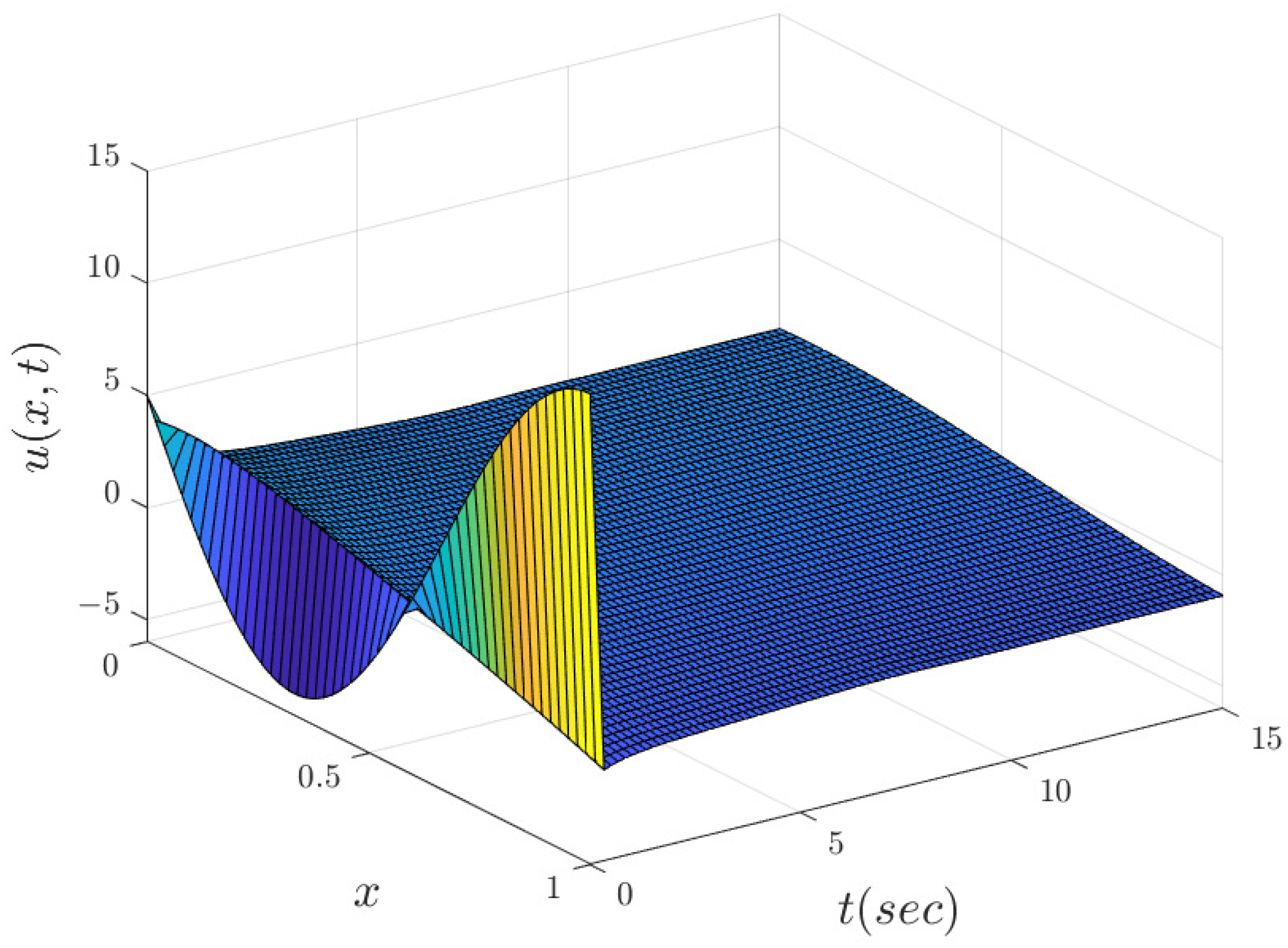
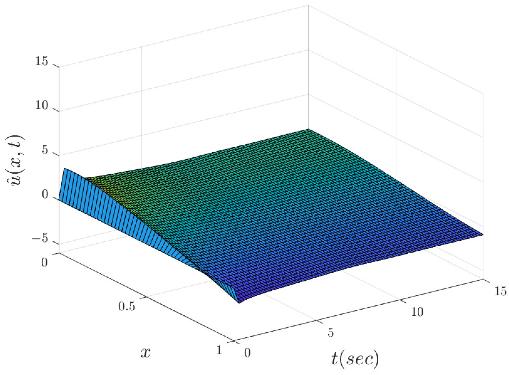
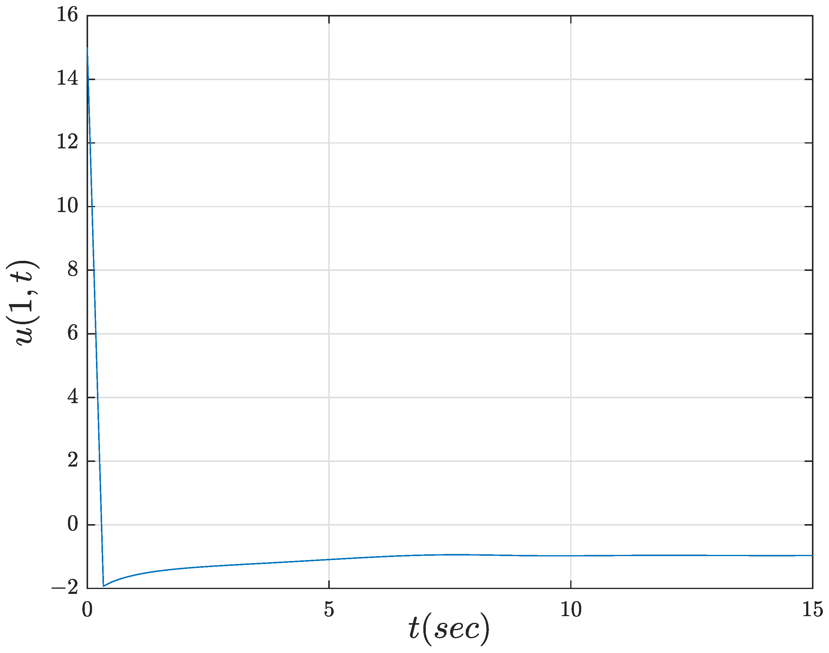
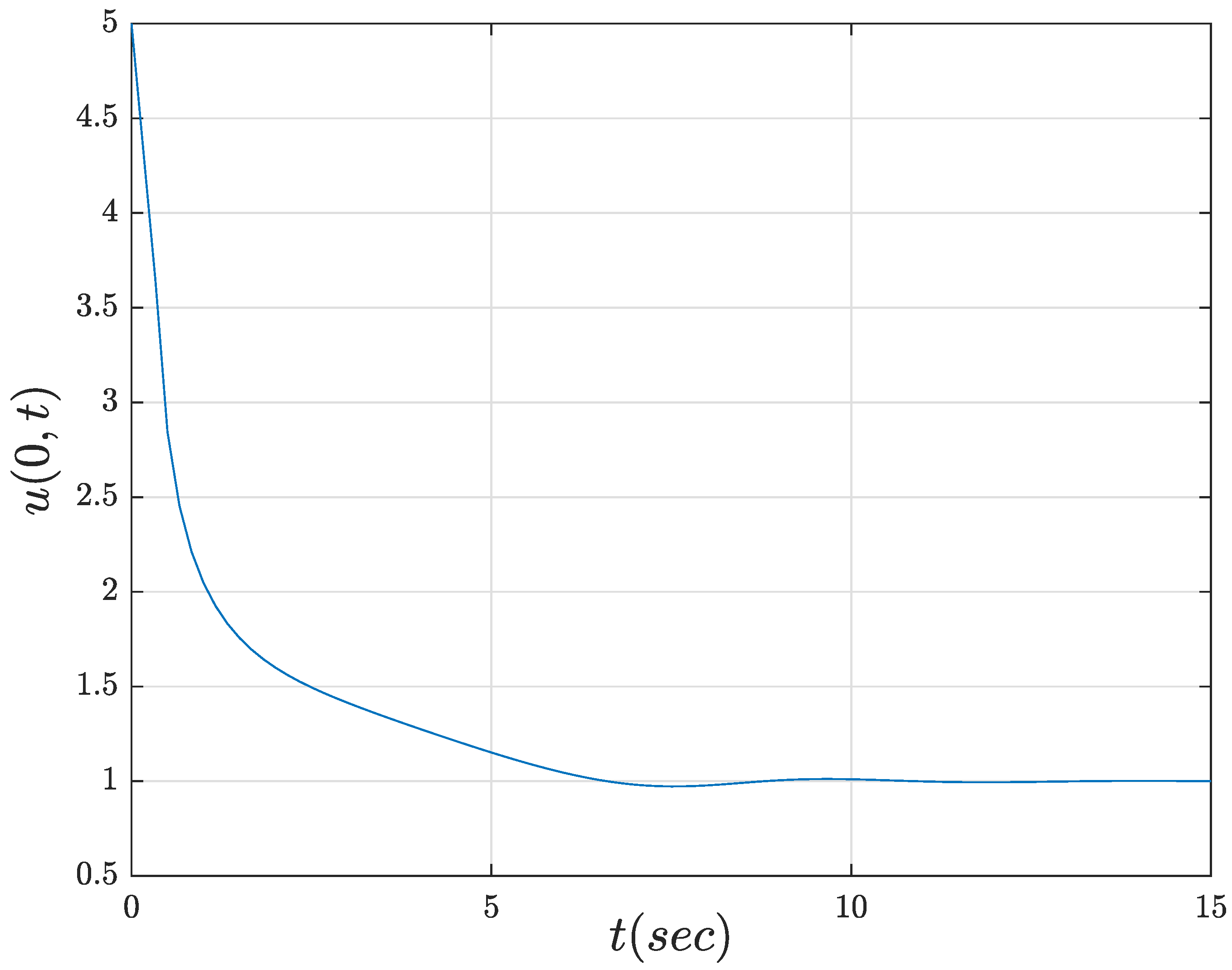
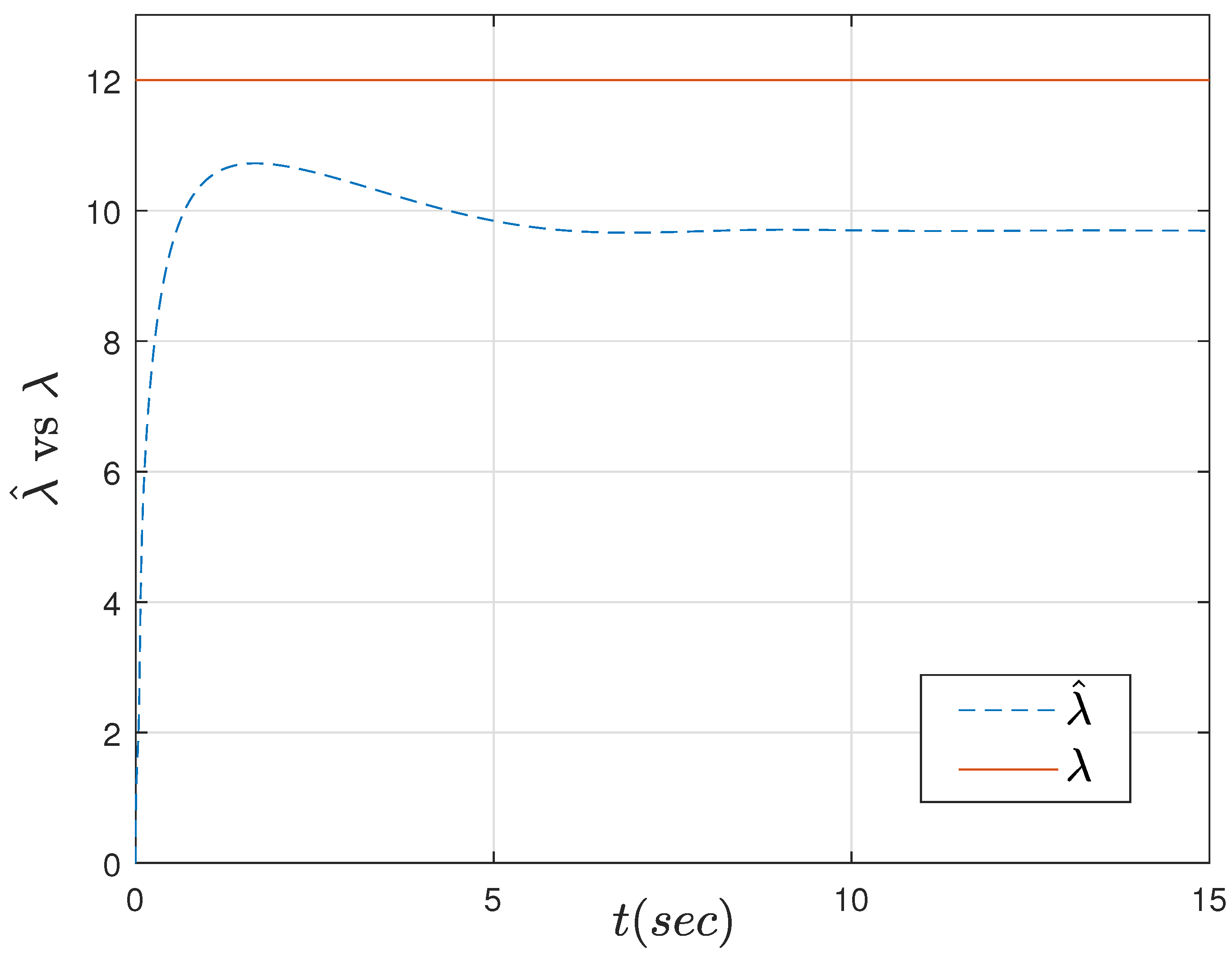
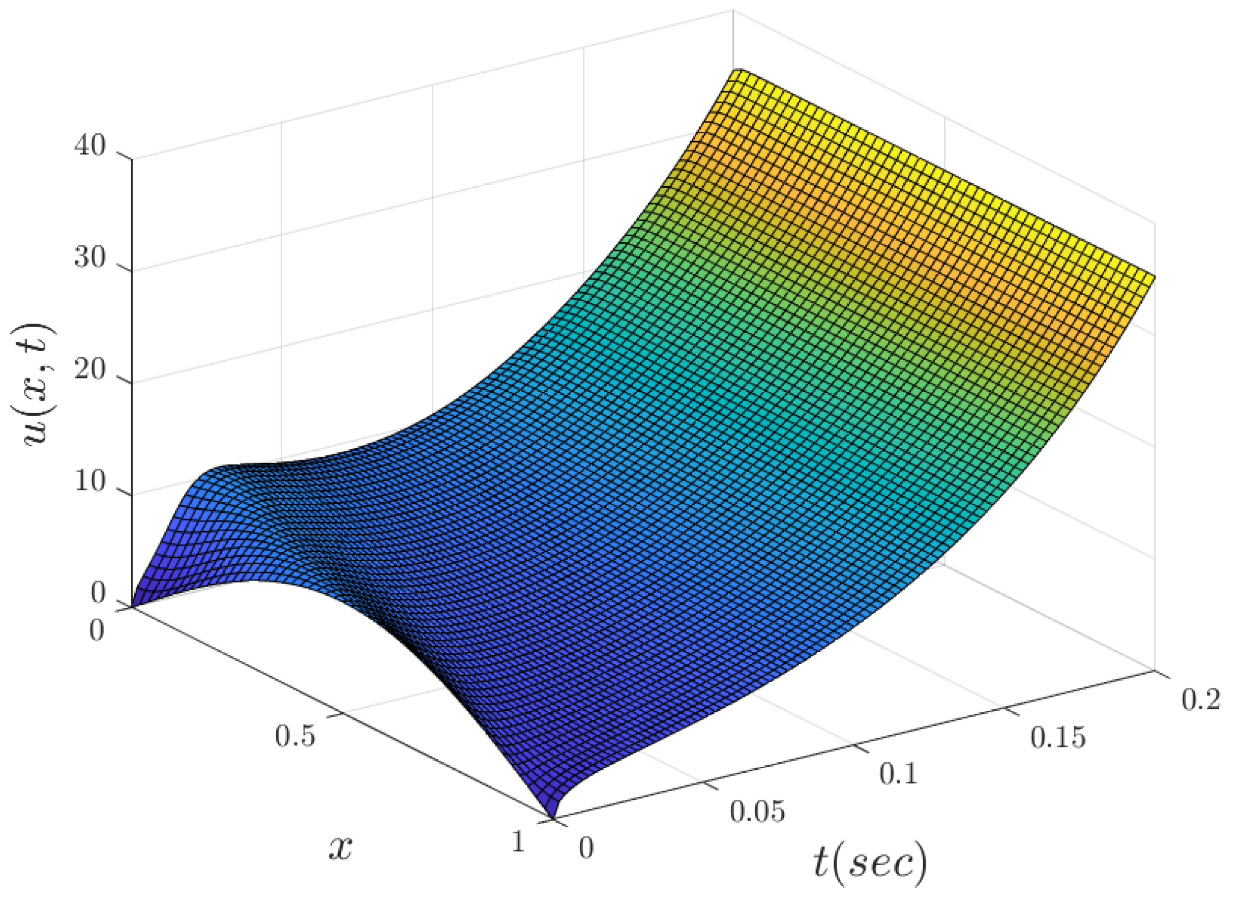
The response of the adaptive BBC is verified via numerical solution. The parameters and gains are set to $b=2$, $\lambda =12$, $\gamma =1$, ${\gamma }_1=25$, ${\gamma }_2=5$ and $u_0\left(x\right)=10sin\left(\pi x\right)$. Although $ϵ$ can be set to different values from the unity, results from studying the stabilization of the unstable shock equilibrium profiles from the Burgers’ equation are not dependent from $ϵ$ in a crucial form. Instead, $ϵ$ just affects the actual size of the estimate for the region of attraction of the closed-loop system. Most of the works on control of PDEs consider $ϵ$ as unity values for numerical simplicity. So, from all of the above, in our study $ϵ$ is settled also as having a unity value. Figure 2 shows the solution in the open-loop of the modified Burgers’ equation when considering the instability term. The solution in open-loop of the modified Burgers’ equation without considering the instability term is depicted in Figure 3. Figure 4 shows the closed-loop dynamics of the system, while Figure 5 shows the dynamics for the identifier PDE. Convergence to zero from the estimation error is shown in Figure 6. The effort of the control signal is depicted in Figure 7. Dynamics of the closed-loop system at the boundaries is depicted in Figure 8 and Figure 9. Figure 10 and Figure 11 show the evolution along time for the parametric estimates, which are bounded and converge near to their ideal values.

9. Discussion

From our study, we realize that the parametric estimates are bounded and converge near their (unknown) ideal values in spite of the fact that the adaptive laws were not designed for invoking the Lyapunov’s method under the tracking dynamics formulated here, and furthermore, the adaptive control law is not based on the structure for that nominal controller, which may be designed directly from the modified Burgers’ system following the BBC methodology. Also, the estimation error converges to zero; meanwhile, the PDE system is stabilized at the boundaries, and the latter are near zero. Clearly, there is no guarantee that the estimated parameters and the estimation error be bounded under our proposal. So, the design of a BBC law based on the model for the modified Burgers’ system is an open problem as well as, consequently, the design of its corresponding adaptive version.

10. Conclusions

In our work, an adaptive BBC is proposed to control a modified Burgers’ system, namely, a nonlinear PDE system, with BCs of the Robin and Neumann types and under the criteria of parametric uncertainties of the convective (nonlinear) and reaction terms. Although the nominal controller is designed from a RAD system, under the assumption that this nominal controller also achieves stabilization for the modified Burgers’ equation, then its adaptive version is proposed for the control of such nonlinear PDE system. This last assumption arises from the comparison of the structure for the modified Burgers’ equation with that from the RAD equation which, in certain sense, looks very similar, in addition to the fact that some controllers designed from the linearization of a finite-dimensional nonlinear system work well for the same nonlinear system, although around an operation point, and that some controllers designed from lower-order systems also work well with higher-order systems. Simulation results show convergence for the parametric estimates near the (unknown) ideal values aside from the convergence of the estimation error to zero. So, we concluded that our proposal performs well with this class of nonlinear PDE system, and further, it can be used in high-dimension and real problems.

References

1. Evans, L.C. Partial Differential Equations, 2nd ed.; American Mathematical Society: Providence, RI, USA, 2010. [Google Scholar]
2. Koga, S.; Krstić, M. Materials Phase Change PDE Control & Estimation: From Additive Manufacturing to Polar Ice; Springer Birkhäuser: Cham, Switzerland, 2020. [Google Scholar]
3. Yu, H.; Krstić, M. Traffic Congestion Control by PDE Backstepping; Springer Birkhäuser: Cham, Switzerland, 2022. [Google Scholar]
4. Anfinsen, H.; Aamo, O.M. Adaptive Control of Hyperbolic PDEs; Springer: Cham, Switzerland, 2019. [Google Scholar]
5. Paunonen, L.; Meurer, T. IEEE Control Systems Society Technical Committee on Distributed Parameter Systems. IEEE Control Syst. 2023, 43, 18–20. [Google Scholar] [CrossRef]
6. Della Santina, C.; Duriez, C.; Rus, D. Model-Based Control of Soft Robots. IEEE Control Syst. 2023, 43, 30–65. [Google Scholar] [CrossRef]
7. Strauss, W.A. Partial Differential Equations: An Introduction, 2nd ed.; John Wiley & Sons: Hoboken, NJ, USA, 2007. [Google Scholar]
8. Byrnes, C.I.; Gilliam, D.S.; Shubov, V.I. Boundary control for a viscous Burgers’ equation. In Identification Control for Systems Governed by Partial Differential Equations; Banks, H.T., Fabiano, R.H., Ito, K., Eds.; SIAM: Philadelphia, PA, USA, 1993. [Google Scholar]
9. Guenther, R.B.; Lee, J.W. Partial Differential Equations of Mathematical Physics and Integral Equations; Dover: Mineola, NY, USA, 1996. [Google Scholar]
10. Krstić, M. On Global Stabilization of Burgers’ Equation by Boundary Control. In Proceedings of the 37th IEEE Conference on Decision and Control, Tampa, FL, USA, 18 December 1998; pp. 3498–3499. [Google Scholar]
11. Gustafson, K.E. Introduction to Partial Differential Equations and Hilbert Space Methods, 3rd ed.; Dover: Mineola, NY, USA, 1999. [Google Scholar]
12. Polyanin, A.D.; Zaitsev, V.F. Handbook of Nonlinear Partial Differential Equations, 2nd ed.; CRC Press: Boca Raton, FL, USA, 2012. [Google Scholar]
13. Humi, M. Introduction to Mathematical Modeling; CRC Press: Boca Raton, FL, USA, 2017. [Google Scholar]
14. Tian, Q.; Yang, X.; Zhang, H.; Xu, D. An implicit robust numerical scheme with graded meshes for the modified Burgers model with nonlocal dynamic properties. Comput. Appl. Math. 2023, 42, 246. [Google Scholar] [CrossRef]
15. Yang, X.; Wu, L.; Zhang, H. A space-time spectral order sinc-collocation method for the fourth-order nonlocal heat model arising in viscoelasticity. Appl. Math. Comput. 2023, 457, 651–674. [Google Scholar] [CrossRef]
16. Zhang, H.; Liu, Y.; Yang, X. An efficient ADI difference scheme for the nonlocal evolution problem in three-dimensional space. J. Appl. Math. Comput. 2023, 69, 651–674. [Google Scholar] [CrossRef]
17. Zhang, H.; Yang, X.; Tang, Q.; Xu, D. A robust error analysis of the OSC method for a multi-term fourth-order sub-diffusion equation. Comput. Math. Appl. 2022, 109, 180–190. [Google Scholar] [CrossRef]
18. Krstić, M.; Smyshlyaev, A. Boundary Control for PDEs: A Course on Backstepping Designs; SIAM: Philadelphia, PA, USA, 2008. [Google Scholar]
19. Krstić, M.; Smyshlyaev, A. Boundary Control of PDEs: The Backstepping Approach. In The Control Handbook, 2nd ed.; Levine, W.S., Ed.; CRC Press: Boca Raton, FL, USA, 2011. [Google Scholar]
20. Krstić, M.; Magnis, L.; Vazquez, R. Nonlinear Control of the Burgers PDE-Part I: Full-State Stabilization. In Proceedings of the 2008 American Control Conference, Seattle, WA, USA, 11–13 June 2008; pp. 285–290. [Google Scholar]
21. Krstić, M.; Magnis, L.; Vazquez, R. Nonlinear Stabilization of Shock-Like Unstable Equilibria in the Viscous Burgers PDE. IEEE Trans. Autom. Control 2008, 53, 1678–1683. [Google Scholar] [CrossRef]
22. Krstić, M.; Magnis, L.; Vazquez, R. Nonlinear Control of the Burgers PDE-Part II: Observer Design, Trajectory Generation, and Tracking. In Proceedings of the 2008 American Control Conference, Seattle, WA, USA, 11–13 June 2008; pp. 3076–3081. [Google Scholar]
23. Kobayashi, T. Adaptive regulator design of a viscous Burgers’ system by boundary control. IMA J. Math. Control. Inf. 2001, 18, 427–437. [Google Scholar] [CrossRef]
24. Morris, K. Control of Systems Governed by Partial Differential Equations. In The Control Handbook, 2nd ed.; Levine, W.S., Ed.; CRC Press: Boca Raton, FL, USA, 2011. [Google Scholar]
25. Aulisa, E.; Gilliam, D. A Practical Guide to Geometric Regulation for Distributed Parameter Systems; CRC Press: Boca Raton, FL, USA, 2016. [Google Scholar]
26. Hong, K.S.; Bentsman, J. Direct Adaptive Control of Parabolic Systems: Algorithm Synthesis and Convergence and Stability Analysis. IEEE Trans. Autom. Control 1994, 39, 2018–2033. [Google Scholar] [CrossRef]
27. Orlov, Y.V. Model Reference Adaptive Control of Distributed Parameter Systems. In Proceedings of the 36th IEEE Conference on Decision and Control, San Diego, CA, USA, 12 December 1997; pp. 263–268. [Google Scholar]
28. Böhm, M.; Demetriou, M.A.; Reich, S.; Rosen, I.G. Model Reference Adaptive Control of Distributed Parameter Systems. SIAM J. Control Optim. 1998, 36, 33–81. [Google Scholar] [CrossRef]
29. Liu, W.J.; Krstić, M. Adaptive control of Burgers’ equation with unknown viscosity. Int. J. Adapt. Control Signal Process. 2001, 15, 745–766. [Google Scholar] [CrossRef]
30. Krstić, M. Lyapunov Adaptive Stabilization of Parabolic PDEs-Part I: A Benchmark for Boundary Control. In Proceedings of the 44th IEEE Conference on Decision and Control, Seville, Spain, 12–15 December 2005; pp. 3164–3169. [Google Scholar]
31. Krstić, M. Lyapunov Adaptive Stabilization of Parabolic PDEs-Part II: Output Feedback and Other Benchmark Problems. In Proceedings of the 44th IEEE Conference on Decision and Control, Seville, Spain, 12–15 December 2005; pp. 3170–3175. [Google Scholar]
32. Smyshlyaev, A.; Krstić, M. Output–Feedback Adaptive Control for Parabolic PDEs with Spatially Varying Coefficients. In Proceedings of the 45th IEEE Conference on Decision and Control, San Diego, CA, USA, 13–15 December 2006; pp. 3099–3104. [Google Scholar]
33. Smyshlyaev, A.; Krstić, M. Lyapunov Adaptive Boundary Control for Parabolic PDEs with Spatially Varying Coefficients. In Proceedings of the American Control Conference, Minneapolis, MN, USA, 14–16 June 2006; pp. 41–48. [Google Scholar]
34. Smyshlyaev, A.; Krstić, M. Adaptive boundary control for unstable parabolic PDEs-Part II: Estimation-based designs. Automatica 2007, 43, 1543–1556. [Google Scholar] [CrossRef]
35. Smyshlyaev, A.; Krstić, M. Adaptive boundary control for unstable parabolic PDEs-Part III: Output feedback examples with swapping identifiers. Automatica 2007, 43, 1557–1564. [Google Scholar] [CrossRef]
36. Krstić, M.; Smyshlyaev, A. Adaptive Boundary Control for Unstable Parabolic PDEs—Part I: Lyapunov Design. IEEE Trans. Autom. Control 2008, 53, 1575–1591. [Google Scholar] [CrossRef]
37. Morris, K.A. Controller Design for Distributed Parameter Systems; Springer: Cham, Switzerland, 2020. [Google Scholar]
38. Krstic, M. On global stabilization of Burgers’ equation by boundary control. Syst. Control Lett. 1999, 37, 123–142. [Google Scholar] [CrossRef]
39. Balogh, A.; Krstić, M. Burgers’ equation with nonlinear boundary feedback: H1 stability, well posedness, and simulation. Math. Probl. Eng. 2000, 6, 189–200. [Google Scholar] [CrossRef]
40. Liu, W.J.; Krstić, M. Backstepping boundary control of Burgers’ equation with actuator dynamics. Syst. Control Lett. 2000, 41, 291–303. [Google Scholar] [CrossRef]
41. Temam, R. Infinite-Dimensional Dynamical Systems in Mechanics and Physics; Springer: New York, NY, USA, 1998. [Google Scholar]
42. Cruz-Quintero, E.; Jurado, F. Boundary Control for a Certain Class of Reaction-Advection-Diffusion System. Mathematics 2020, 8, 1854. [Google Scholar] [CrossRef]
43. Smyshlyaev, A.; Krstić, M. Adaptive Control of Parabolic PDEs; Princeton University Press: Princeton, NJ, USA, 2010. [Google Scholar]
44. Abramowitz, M.; Stegun, I.A. Handbook of Mathematical Functions: With Formulas, Graphs, and Mathematical Tables; Dover Publications: Mineola, NY, USA, 1965. [Google Scholar]
45. Zachmanoglou, E.C.; Thoe, D.W. Introduction to Partial Differential Equations with Applications; Dover: Mineola, NY, USA, 1986. [Google Scholar]
46. Arfken, G.B.; Weber, H.J.; Harris, F.E. Mathematical Methods for Physicists: A Comprehensive Guide, 7th ed.; Academic Press: Waltham, MA, USA, 2013. [Google Scholar]
47. Ioannou, P.A.; Sun, J. Robust Adaptive Control; Prentice Hall: Englewood Cliffs, NJ, USA, 1995. [Google Scholar]
48. Murillo-García, O.F.; Jurado, F. Adaptive Boundary Control for a Certain Class of Reaction-Advection-Diffusion System. Mathematics 2021, 9, 2224. [Google Scholar] [CrossRef]
Figure 1. Adaptive BBC scheme for the modified Burgers’ system (124)–(126).
Fractalfract 07 00834 g001
Figure 2. Solution of the modified Burgers’ system when including the instability term.
Fractalfract 07 00834 g002
Figure 3. Solution of the modified Burgers’ system in absence of the instability term.
Fractalfract 07 00834 g003
Figure 4. Performance of the adaptive controller.
Fractalfract 07 00834 g004
Figure 5. Response from the identifier PDE.
Fractalfract 07 00834 g005
Figure 6. Estimation error.
Fractalfract 07 00834 g006
Figure 7. Control effort of the adaptive controller.
Fractalfract 07 00834 g007
Figure 8. Dynamics of the closed-loop system at the boundary x = 1 .
Fractalfract 07 00834 g008
Figure 9. Dynamics of the closed-loop system at the boundary x = 0 .
Fractalfract 07 00834 g009
Figure 10. Evolution of the parametric estimate λ ^ .
Fractalfract 07 00834 g010
Figure 11. Evolution of the parametric estimate b ^ .
Fractalfract 07 00834 g011
Disclaimer/Publisher’s Note: The statements, opinions and data contained in all publications are solely those of the individual author(s) and contributor(s) and not of MDPI and/or the editor(s). MDPI and/or the editor(s) disclaim responsibility for any injury to people or property resulting from any ideas, methods, instructions or products referred to in the content.