Abstract
The capacity regeneration phenomenon is often overlooked in terms of prediction of the remaining useful life (RUL) of LIBs for acceptable fitting between real and predicted results. In this study, we suggest a novel method for quantitative estimation of the associated uncertainty with the RUL, which is based on adaptive fractional Lévy stable motion (AfLSM) and integrated with the Mellin–Stieltjes transform and Monte Carlo simulation. The proposed degradation model exhibits flexibility for capturing long-range dependence, has a non-Gaussian distribution, and accurately describes heavy-tailed properties. Additionally, the nonlinear drift coefficients of the model can be adaptively updated on the basis of the degradation trajectory. The performance of the proposed RUL prediction model was verified by using the University of Maryland CALEC dataset. Our forecasting results demonstrate the high accuracy of the method and its superiority over other state-of-the-art methods.
1. Introduction
The increasing demand for lithium-ion batteries (LIBs) necessitates high reliability and safety requirements for their operation. As a result, it is crucial to have an effective method for predicting the remaining useful life (RUL) [1,2,3].
A number of studies have investigated the problem of RUL prediction and health state estimation of LIBs from various viewpoints [4,5,6]. Many of these studies rely on numerical prediction and provide a single predicted value. For instance, Zhao et al. [7] developed a fusion neural network model that combines a generalized learning system algorithm with a long short-term memory neural network (LSTM) to predict the capacity and RUL of Li-ion batteries. Li et al. [8] employed convolutional neural networks and transfer learning to implement online capacity estimation of LIBs. Other researchers developed methods based on a combination of different RUL models to overcome the limitations of a single model [9,10,11].
However, numerical predictions often fail to adapt to different practical application scenarios. Moreover, battery degradation trajectories are complex and highly nonlinear, posing challenges in developing accurate RUL prediction models [12]. Then the RUL prediction model should not only accurately determine the future degradation of LIBs but also possess flexibility and adaptability to the specific conditions and provide an assessment of the uncertainty [13,14,15].
In order to quantify the uncertainty of prediction results, deep learning methods can be combined with dropout techniques [13] and Monte Carlo methods [14]. For instance, Li et al. [16] utilized a long short-term memory neural network for RUL prediction of LIBs and employed the dropout method to quantify prediction uncertainty. Similarly, Liu et al. [17] developed a method combining Bayesian model averaging with long- and short-term memory neural networks. Multiple neural network models were constructed to obtain different prediction results, and Bayesian model averaging was used to estimate the posteriori distribution of the predictions, generating confidence intervals that reflect the uncertainty. However, these techniques rely on a substantial amount of high-quality data to effectively train the prediction models. Moreover, the interpretability of these models is limited, and ensuring their generalization ability poses a challenge [18].
Statistics-based approaches for the prediction of RUL rely on probability theory and the statistical principles of historical data. These approaches provide interpretable prediction models and can be applied with minimal data quantity requirements and low quality [19]. Additionally, they provide for the quantification of prediction uncertainty in the form of probability distributions. For example, Xu et al. [20] combined the Wiener process with the Bayesian method to predict the RUL of LIBs. They established a local fluctuation fitting model that partitioned the normal degradation trend and the local fluctuation component. The Bayesian method was then used to update the predicted life probability density function online. However, these common methods have limitations. One such limitation is that the degradation increments are considered independent, implying that the degradation process described by these methods is memoryless [21]. To address this, Wang et al. [22] proposed a RUL estimation method for LIBs based on fractional Brownian motion (fBM), utilizing a Drosophila optimization algorithm for the Hurst index. Hong et al. [23] developed a fractional-order generalized Cauchy process-based fGC model for RUL prediction of Li-ion batteries and employed Monte Carlo simulation to obtain the lifetime probability density function. However, these degradation models can only describe degradation processes that adhere to a Gaussian distribution and lack flexibility for non-Gaussian time series.
Figure 1 illustrates the capacity curve for cell CS2_36, representative of the CALCE dataset’s CX2 series, under a standard charging regime. The cells experienced a constant current charge at 0.5 C to 4.2 V, followed by constant voltage until the current declined to below 0.05 A, and a consistent discharge cut-off at 2.7 V. The blue line in the figure traces the anticipated monotonic capacity decline under typical degradation conditions. In contrast, the red line captures deviations from this norm, manifesting as sporadic capacity increases attributable to regeneration events and stochastic fluctuations. Such patterns reflect a complex degradation process not confined to Gaussian behavior, hence the application of Lévy stable motion to model the observed anomalies. This approach, with its heavy-tailed statistical properties, effectively captures abrupt transitions in battery capacity degradation [24]. This technique is suitable for capturing sudden jumps in degradation processes. Liu et al. [25] employed incremental distribution with fractional Lévy stable motion to establish an iterative predictive model by using Monte Carlo simulation. This model primarily addresses non-Gaussian characteristics of the degradation process. However, a drawback of the model is that it assumes that the drift coefficients follow a normal distribution and are not dynamically updated. This limitation significantly affects the accuracy of RUL predictions for lithium-ion battery devices.
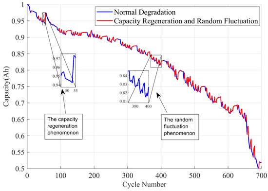
Figure 1.
Degradation process of lithium-ion batteries.
The main results of this study can be summarized as follows:
(1) In order to address the capacity regeneration phenomenon and random fluctuation in the degradation process of LIBs, fractional Lévy stable motion with an adaptive nonlinear drift model is proposed. This model takes into account the non-Gaussian nature of the degradation process and enables adaptive optimization of drift coefficients based on the degradation path. By considering the influence of historical observation data, the model can better capture the complex dynamics of the degradation process and improve the accuracy of its predictions.
(2) The RUL distribution is provided as a semi-analytical solution by utilizing the Mellin–Stieltjes transform and the Monte Carlo method. This approach gives accurate results and saves computational time compared to direct Monte Carlo simulation for calculating the RUL probability density function. Additionally, a genetic algorithm was employed to optimize the resampling process in the filtering algorithm. This approach effectively addresses the issue of particle depletion and significantly improves the prediction accuracy of the model.
(3) The proposed model is validated on the University of Maryland lithium-ion battery CACLE dataset. The results demonstrate that the method overcomes other state-of-the-art techniques in terms of the accuracy of the RUL prediction, specifically considering capacity regeneration and random fluctuations.
In Section 2, the paper provides a comprehensive explanation of the proposed RUL prediction model, outlining its key elements and methodology. Section 3 focuses on discussing the various techniques employed for the parameter estimation of the model. In Section 4, we describe a case study, showcasing the application of the proposed model and the estimation of its performance characteristics. Finally, Section 5 summarizes the findings and conclusions of the study.
2. Proposed Methodology for RUL Prediction
2.1. Long-Range Dependence of Fractional Lévy Stable Motion
Let be a random variable that is said to follow a Lévy stable distribution if, for any independent copies of and any positive constants , parameters and exists, such that:
Here, and are not arbitrary but are calculated to satisfy the distribution’s stable property. The symbol signifies that the distribution of the linear combination is identical to that of , scaled by and shifted by . This stability under linear combinations of independent copies is the defining characteristic of the Lévy stable distribution, ensuring that the scaled sum maintains the same probabilistic properties as the original variable .
Due to the nature of the Lévy stable distribution, there is no analytical expression for the probability density function in closed form. As a result, the properties of the Lévy stable distribution are typically expressed through its characteristic function . which is defined as follows [26]:
A process described by random variables depends on the stable index , skew index , drift coefficient , and diffusion parameter . Values of and influence the shape of the distribution, whereas and determine the linear transformation of the distribution. Recall that the parameters of Equation (2) must satisfy the following conditions: , , , and . These constraints ensure that the stable index, skew index, and diffusion parameter are within their valid ranges, allowing for a meaningful representation of the Lévy stable distribution.
In the degradation process of LIBs, available capacity does not exhibit a strict monotonic decrease. Instead, it alternates between sudden increases and gradual decreases due to the presence of random fluctuations and capacity regeneration phenomena. Consequently, the decay rate deviates from the Gaussian assumption. Figure 2 shows the fitting of the capacity degradation rate distribution by using the dataset obtained from the CS2-36 battery [27,28,29]. Different fitting curves clearly demonstrate that a steady-state distribution is more relevant for our simulation. This observation emphasizes the importance of Levy stable distribution for a precise description of the degradation trend.
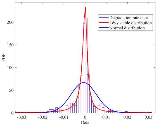
Figure 2.
Comparison of fitting methods for prediction of capacity degradation distribution.
Fractional Lévy stable motion can be defined by the following stochastic integral [30],
where ; and ; and is the Lévy stable measure in the Lebesgue measure space. The fLSM model serves as an extension of the fBM model, and they have many similar and different properties; when , the fLSM model degenerates to the fBM model. The relevant properties of the fLSM model are determined by the relationship between and . The fLSM model has the LRD property when ; when , the fLSM model has the SRD property; and when , the fLSM model degenerates to the LSM model.
2.2. Analysis of Performance Degradation
In our study, Equation (4) serves as a generalized form of fractional Brownian motion [25], tailored to capture the dynamics of fractional Lévy stable motion:
where denotes the degenerative process, is the drift coefficient, is the diffusion parameter, and both and are constants. is an fLSM, where denotes the increment of Lévy movement. This formulation is particularly adept at modeling the non-Gaussian behaviors observed in complex systems, showcasing the utility of fLSM in exploring and understanding the intricate dynamics that traditional Gaussian models may fail to capture [26].
The overall trend of the capacity degradation process implies that the drift term is a time-dependent function. Additionally, the degradation process is influenced by uncertain LRD fluctuations, characterized by the diffusion term. Consequently, the drift and diffusion terms in Equation (5) can be generalized as follows:
where is the initial value of degradation and is the drift coefficient at time , indicating the degradation rate. The diffusion term is driven by the fLSM with a diffusion coefficient of and takes into account the effect of signal noise.
In order to estimate the parameters in the model and the subsequent RUL predictions, the form of the incremental distribution of the degenerate model is to be derived. The first differencing of the degenerate model leads to the following equation [31]:
In order to obtain a concrete expression of the degenerate model, it is necessary to specify . Because fLSM increment is also a self-similar process and satisfies the following equation:
In order to obtain an expression of the degenerate model, it is necessary to specify . Since fLSM increment is a self-similar process and satisfies the identity
according to the Maruyama model:
and according to Equations (22) and (23), it can be concluded that
where is the Lévy stable distribution of white noise, whose distribution obeys .
Furthermore, based on the linear nature of the symmetric Lévy stable distribution of white noise , the following operation relationship must be introduced:
where and are the nonzero constant and real numbers, respectively. According to the property description of (12), Equation (13) below holds:
2.3. Adaptive Evaluation of Nonlinear Drift Coefficient
In order to improve the accuracy of the RUL prediction, it is essential to update the time-dependent value of the drift coefficient. To achieve this goal, we construct the following state-space model:
where Equation (14) represents the state equation and Equation (15) represents the observation equation. is the Gaussian-distributed state noise with variance . The choice of the drift term function depends on the historical degradation trajectory. In this paper, the power-law drift model is adopted, where parameters and are determined by nonlinear least-squares estimation. The superscript or subscript indicates the observation time.
The following describes how the drift term is adaptively updated:
Step 1. Initialization
Initialize the prior distribution , the number of particles M, the number of iterations N. Set k = 1, , , , . Here, is the particle set matrix, is the diffusion term, and is the vector of predicted values, related to the observed values vector .
Step 2. Generation of particle set matrix
The particle set matrix are calculated as follows:
where is the importance density, which avoids the difficulty of sampling directly from the prior PDF, and represents the i-th particle of the k-th iteration.
Step 3. Prediction of particle sets based on observations
The prediction based on the observation, for each particle is computed as
where is the i-th predicted value of the k-th iteration for the current particle.
Step 4. Calculation of particles weights
The weight of each particle is calculated as
Here, is the weight for the i-th particle of the k-th iteration, and is a small positive real number.
Then, the normalization of each weight is computed as follows:
where is the normalized weight for the i-th particle of the k-th iteration.
Step 5. Resampling based on genetic algorithm optimization
The normalized particle weights obtained in step 4 are first processed by binary coding. Selection operations can avoid reducing good genes and improve global convergence. In this paper, we choose the roulette selection method, i.e., generate a random number between 0 and 1. When falls in the particle interval, the particle will be copied as a parent particle. In the selection operator operation, is the adaptation rate, and the following equation holds:
The following crossover operation is performed, and the crossover method used in this section is a single-point crossover, by performing this operation, the searching ability of the genetic algorithm can be greatly improved. In this operation, two particles and exchange some of their genes with each other in a single-point manner to produce two new offspring particles, where k satisfy and n satisfy . is the crossover rate and satisfies the following equation:
After performing the mutation creation, a decimal decoding operation is performed on the parent and child particles to obtain the weights .
Step 6. Output
The estimated value of the adaptive drift coefficient λ is calculated as
where is the estimated drift coefficient at time and E() denotes the expectation. Based on the estimated adaptive drift coefficient at moment , the predicted value of the degradation process can be expressed as
Here, is the predicted value for the degradation process at the time .
2.4. Semi-Analytic Solution of the RUL Distribution for AfLSM Prediction Models
The accurate selection of appropriate operating parameters for LIBs is essential, as these parameters indirectly impact the prediction accuracy of RUL and the applicability of the prediction model. In this paper, the capacity regeneration and random fluctuation phenomena observed in the degradation process of LIBs are taken into account. To define a health factor that considers these phenomena, the capacity degradation rate is utilized after normalizing the available capacity. The capacity degradation rate, in this context, represents the rate at which the capacity of the battery decreases over time, reflecting its health condition, which is defined as follows:
where denotes the health state of the lithium-ion battery of the i-th cycle, denotes the available capacity in the i-th cycle, and denotes the initial capacity.
In the above equation, y denotes the capacity degradation rate of the lithium-ion battery.
In this paper, we define the RUL based on the first arrival time:
where is the current time of the degradation process, is the time of RUL, is the prediction starting point FPT, and is the set fault threshold.
Form Equations (13) and (26), it can be obtained as
where is the hidden state variable at time , and it can be updated based on monitoring data. Therefore, in order to facilitate the solution of the RUL of the prediction model, the boundary values of the RUL should be considered, i.e., equal on the left and right sides of Equation (27).
Therefore, our goal becomes to solve for in the equation
Transcendental Equation (28) has no analytical solution.
By using the Mellin–Stieltjes transform [32], the p-order moments of can be expressed as
where
denotes the gamma function. The gamma function is defined as .
The first-order moments of are considered as ideal solutions and can be obtained as
The second term on the left side of Equation (28) can be expressed as
where the power-law drift model is used as the nonlinear drift function for the performance degradation model. Then, we can solve for the PDF of the RUL by calculating Equations (31) and (32), followed by the Monte Carlo simulation.
Due to the absence of a closed-form PDF for the Lévy distribution, the random sequence generated by the fLSM is non-stationary. As a result, generating RUL values using this random sequence and performing a Monte Carlo simulation can introduce a significant bias. To address this issue, a transcendental equation is considered based on the definition of the first passage time. In this approach, the PDF of the final RUL is obtained through a combination of semi-analytical and numerical Monte Carlo simulation techniques. This allows for a more accurate estimation of the RUL values while accounting for the non-stationarity of the random sequence generated by the fLSM. Figure 3 provides a schematic diagram of the approach, referred to as the AfLSM for RUL prediction. It visually represents the steps involved in obtaining accurate RUL predictions using the proposed methodology.
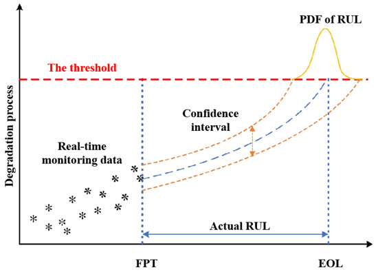
Figure 3.
Schematic diagram of RUL prediction: AfLSM model.
3. Estimation of Degradation Model Parameters
Estimation of long-range dependent and self-similar processes is carried out by the Hurst index , which is independent of other degradation parameters. Thus, the estimation of the Hurst index is carried out independently of other parameters. In this paper, a method called the generalized Hurst exponent method is introduced to estimate the Hurst index accurately. This method provides narrower confidence intervals for the estimation. The generalized Hurst exponent is utilized to examine the scaling properties of the data by considering the q-order moments of the incremental distribution. These moments are associated with long-term dependence and are less influenced by outliers in the data. The expression for the calculation of the Hurst exponent by using the q-order moment method reads as follows [33]:
where is the time series, ⟨·⟩ denotes the average value over the dataset, and denotes the time interval. The generalized Hurst exponent becomes the Hurst exponent for .
The observed values set at are , where k is the number of observations. The incremental process Y of X can be written as ]. From Equation (13) combined with the new eigenfunction method [34], the parameters of the degradation model of AfLSM can be derived. Estimates of the parameters , , and are obtained:
where and indicates the imaginary part of the number.
The flowchart of the RUL prediction framework is shown in Figure 4.
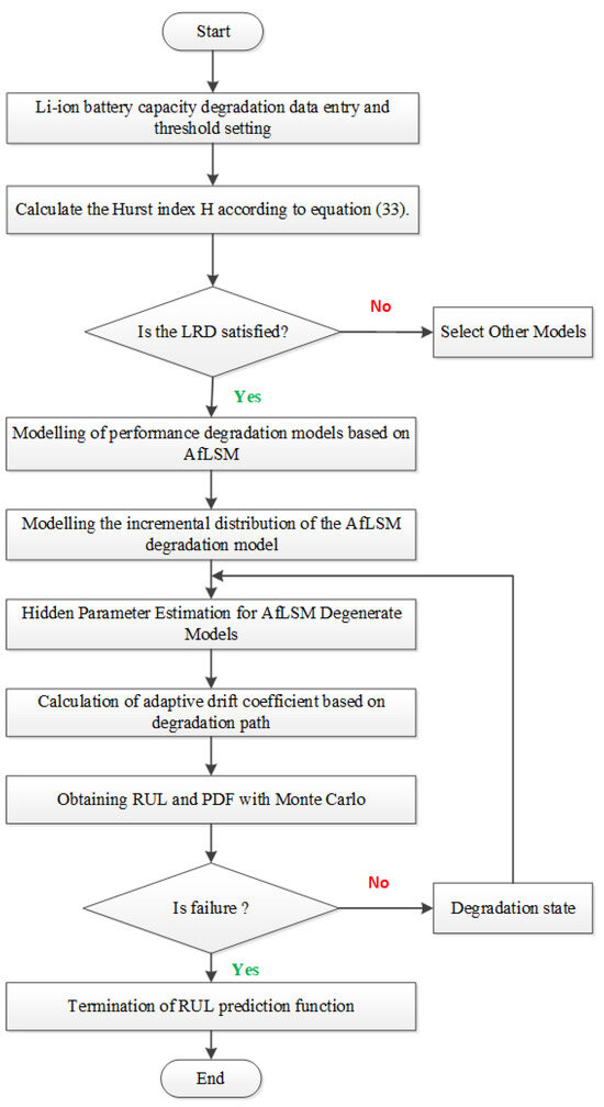
Figure 4.
Flowchart of the proposed RUL prediction framework.
4. Case Study
4.1. Data Sets and Predictive Evaluation Indicators
In order to implement our model, we referred to open-source data from the University of Maryland CALCE. These datasets were obtained from an accelerated aging test conducted on a batch of LIBs with a calibrated capacity of 1.1 Ah.
The cathode of the LIBs in the dataset is composed of lithium-ion cobalt oxide (LiCoO2), while the anode consists of layered graphite with polyvinylidene fluoride. During the accelerated aging test, all the Li-ion batteries were charged at a constant current of 0.55 A until the voltage reached 4.2 V. Subsequently, they were charged at a constant current to maintain the voltage at 4.2 V until the charging current dropped below 50 mA. After the above charging process, batteries CS2_33 and CS2_34 were discharged at a constant current of 0.55 A, while CS2_35, CS2_36, and CS2_38 were discharged at a constant current of 1.1 A until the voltage of the LIBs dropped to 2.7 V. The test concluded when the capacity of the LIBs reached the end-of-life threshold, indicating the point at which they were no longer usable.
In the context of the paper, it is stated that when the capacity of a lithium-ion battery decreases by 20–30%, its performance experiences an exponential decline. As a result, the battery is deemed unreliable once it reaches this threshold. For the purpose of this study, the end-of-life threshold for the LIBs is defined as 76%. This means that when the capacity of a lithium-ion battery drops to 76% of its initial capacity, it is considered to have reached the end of its useful life and is no longer reliable for practical applications.
In order to assess the effect of the RUL prediction model, four evaluation criteria, including health degree, cosine similarity, mean absolute error, and root mean square error, are calculated to reflect the accuracy of RUL results.
The HD is calculated from Equation (37). Higher values of the health degree correspond to better results of the RUL prediction model:
where represents the predicted value of RUL from the ith predictive starting point, is the actual value of RUL at the ith predictive starting point, is the mean value of , and num is the number of predictions.
To measure the degree of similarity, we use the cosine similarity method, which calculates the cosine between two vectors, i.e.,
The MAE is calculated using Equation (39); the smaller its value, the higher the prediction accuracy of the RUL model:
Smaller values of the RMSE indicate higher accuracy:
4.2. RUL Prediction Based on the AfLSM Model
The RUL of the lithium-ion battery is predicted at specific cycle intervals: 321, 361, 401, 441, and 481 cycles. To account for the uncertainty associated with randomly fluctuating health state data, we employ Monte Carlo simulation with 500 simulation trials.
In order to assess the impact of updating the nonlinear drift coefficient on the predictions of the RUL, two models are considered. The first model, referred to as M1, corresponds to the model proposed in Section 2. The second model, denoted as M2, does not consider the nonlinear coefficient drift. The determination of the nonlinear drift coefficient for the M2 model can be referenced from literature sources [25,26].
Figure 5 displays the prediction results of the two models, and Table 1 presents detailed data related to these results. The parameter estimation outcomes for both models are listed in Table 2. Furthermore, Table 3 provides the results of the evaluation indicators.
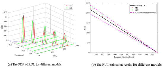
Figure 5.
PDF of AfLSM prediction models with and without adaptive power-law drift terms.

Table 1.
Prediction results of the algorithm based on CS2_36 lithium-ion battery data.
Table 2.
Parameter estimates for the AfLSM prediction model with power-law drift term.
Table 3.
RUL prediction results evaluation for different methods.
From Figure 5, it is evident that the predicted RUL values closely align with the actual RUL values, with the majority of estimated RULs falling within the 90% confidence interval. As the observation time increases, the predicted RUL values converge towards the actual RUL values, and the corresponding PDF curves become increasingly elevated. This indicates that as more observational information and historical data are incorporated, the RUL prediction accuracy improves. Additionally, the higher confidence level associated with the same length of confidence interval enhances the reliability of the prediction results, facilitating real-time RUL prediction.
According to Table 3, model M1, which takes into account the adaptive drift of nonlinear coefficients, exhibits smaller values of RMSE and MAE, as well as larger values of COS and HD, compared to the M2 model, which does not consider the nonlinear drift. These results indicate that the prediction model’s overall performance is improved when the nonlinear coefficients are adaptively updated along the degradation path.
4.3. Comparison and Discussion with Other Methods
In order to emphasize the objectivity and superiority of our results, the method of RUL prediction is compared with representative state-of-the-art methods based on stochastic processes and advanced deep learning models. The corresponding prediction models are shown below.
- (1)
- Method 3 (M3): This is the EMD-LSTM model [35,36], and we also quantify the uncertainty of the MMA-LSTM model by using the Dropout method. The optimal value of Dropout was set to 0.3, the initial learning rate was set to 0.01, the maximum step size was 210, the learning rate reduction factor was 0.4, and the learning rate period was 40.
- (2)
- Method 4 (M4): This is the DCNN model [37,38], and we have also quantified the uncertainty of the DCNN model by using the Dropout method. The optimal value of Dropout is set to 0.2.
- (3)
- Method 5 (M5): This is the fBM model without adaptive drift coefficient λ, and the drift function is . The degradation model satisfies the following formula,
Here, represents the fractional Brownian motion, is the constant diffusion coefficient, and is an adaptive time-varying drift coefficient.
- (4)
- Method 6 (M6): This is the Wiener model with adaptive drift coefficient λ, and the drift function is . The degradation model satisfies the following formula:
Figure 6 illustrates the prediction results of the different models, whereas Table 1 provides corresponding data. The values of the various model assessment indicators are presented in Table 3. The qualitative assessment of the RUL prediction results in Figure 6 indicates that the M1 model provides estimates closer to the true values compared to the other three models. Table 3 confirms this, as the M1 model achieves the smallest MAE and RMSE metrics among all models, indicating higher accuracy in RUL predictions compared to the other models (M3–6). The larger HD value for the M1 model suggests better fitting of the predictions. Additionally, the COS value obtained by M1, closer to 1, indicates greater similarity between the predicted and actual RUL values, resulting in a more stable prediction performance. Furthermore, in Figure 6b, the λ-performance region demonstrates improved prediction accuracy of the AfLSM degradation model for RUL prediction incorporating capacity regeneration and random fluctuation phenomena.
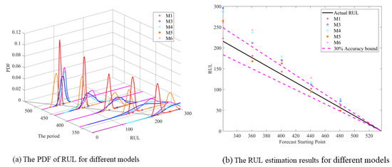
Figure 6.
PDF of the RUL of different prediction models.
Moreover, to assess the uncertainty of the RUL prediction results quantitatively, the PDF curves of the prediction outcomes are thoroughly analyzed and compared throughout the entire performance degradation process of LIBs. The comparison results between the RUL predictions of M1 and those of M3, M4, M5, and M6 are presented in Figure 6 and Figure 7. Observing these figures, it is evident that the PDF curve of the proposed method, referred to as M0, exhibits greater height and steepness compared to the corresponding PDF curves of the other methods. This observation suggests that the RUL prediction model proposed in this paper achieves higher prediction accuracy and reliability.
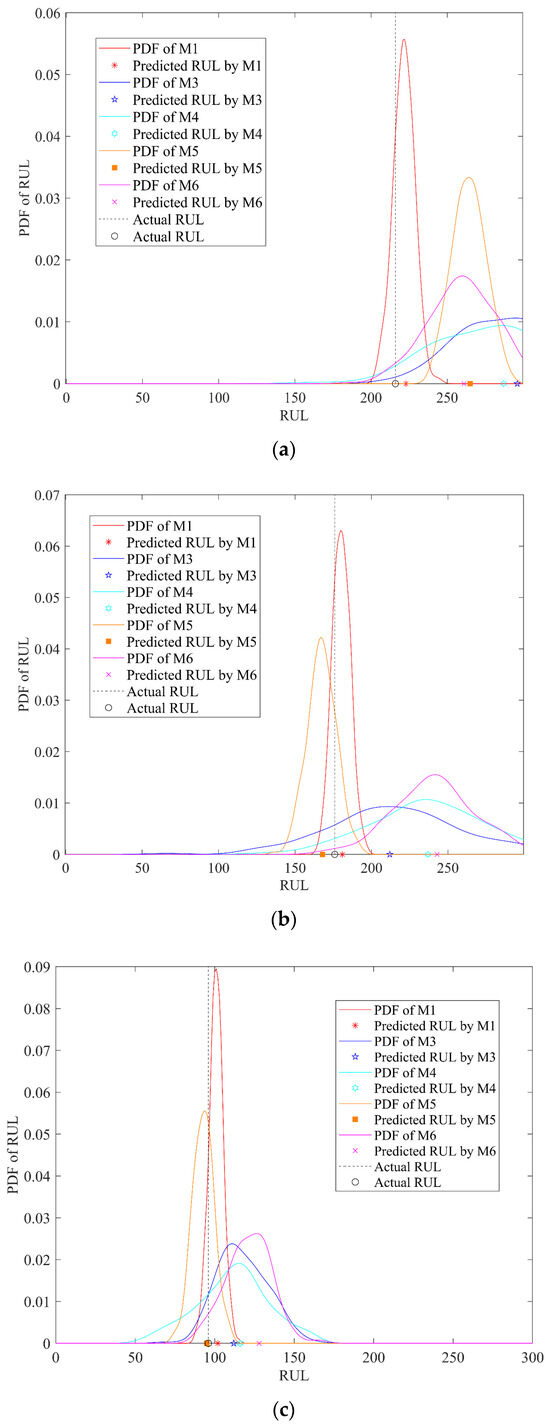
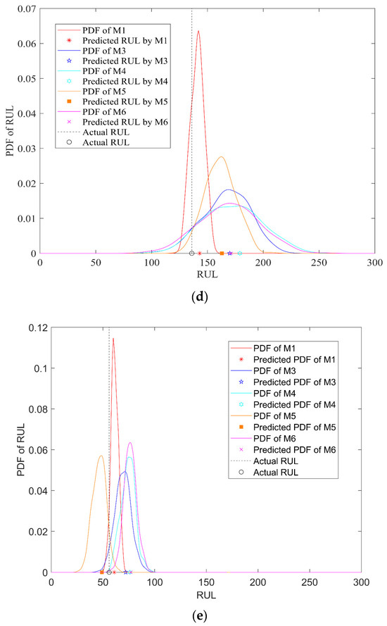
Figure 7.
RUL prediction and PDF analysis for M1, M3, M4, M5, and M6 at different observation times. (a) RUL prediction and PDF analysis with a prediction starting point of 321 cycles; (b) RUL prediction and PDF analysis with a prediction starting point of 361 cycles; (c) RUL prediction and PDF analysis with a prediction starting point of 401 cycles; (d) RUL prediction and PDF analysis with a prediction starting point of 441 cycles; (e) RUL prediction and PDF analysis with a prediction starting point of 481 cycles.
To conduct a comprehensive comparison of the single-point RUL prediction results across different methods, the predictions and corresponding PDF curves are separately analyzed at various observation moments during the degradation of LIBs. The analysis results are depicted in Figure 7. Specifically, Figure 7a–e present the prediction results for five different observation cycle periods: 321, 361, 401, 441, and 481. Upon examining these figures, it is evident that the M1 model proposed outperforms the four models M3–6. This superiority is reflected in the M1 model RUL predictions, which are closer to the actual values indicated by the black dashed lines.
To quantitatively compare and analyze the prediction performance of different models, the logarithmic relative error of the prediction outcomes is calculated using Equation (43):
where is the natural logarithm operation. LRE (logarithmic relative error) represents the logarithmic relative error of the i-th observation. A smaller value of LRE indicates a lower level of prediction error, thus indicating a higher degree of precision in the prediction outcome. To conduct a systematic analysis of the LRE errors of the prediction results, box plots were generated to illustrate the distribution of LRE errors for the four prediction models. The box-and-whisker plot representing this analysis is displayed in Figure 8.
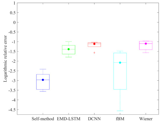
Figure 8.
Box plot of logarithmic relative error for prediction results.
To conduct a systematic analysis of LRE in the prediction results, box plots were generated to illustrate the distribution of LRE errors for the four prediction models. The box-and-line plot is presented in Figure 8. Notably, the SELF method proposed in this paper exhibits a clear minimum median in the box plot and a smaller interquartile range, indicating a more concentrated central tendency and lower volatility in the prediction error distribution compared to the other three assessment methods. Conversely, although the DCNN method has the smallest box plot, the presence of outliers suggests high fluctuations in the prediction errors, leading to unstable prediction results. The EMD-LSTM method and the Wiener method demonstrate larger central values, despite having slightly smaller box plots compared to our proposed method, indicating relatively lower overall accuracy.
The EMD-LSTM method, while capable of capturing the degradation trend from historical data, produces smooth predictions that fail to reflect the characteristics of capacity regeneration and stochastic fluctuation phenomena. The DCNN method typically relies on abundant training data and structured patterns for effective learning and prediction, making it more challenging to handle data with significant stochastic fluctuations. Moreover, the classical stochastic process methods, such as the fBM model and Wiener model, overlook non-Gaussian degradation resulting from the capacity regeneration phenomenon in lithium-ion battery processes. As the number of cycling cycles increases, the accuracy of all methods improves. However, the proposed method consistently demonstrates higher accuracy in comparison with other methods, thereby establishing its superiority in RUL prediction.
5. Conclusions
Numerous studies have been conducted to predict the RUL of LIBs. However, the degradation process of battery capacity is non-monotonic during charging and discharging, posing challenges to the accuracy of RUL prediction for LIBs. The presence of self-capacity regeneration and stochastic fluctuations further complicates the prediction by affecting the average degradation trend of the battery. Moreover, these phenomena are inherent in the daily usage of each battery.
To address these challenges, we propose a lithium-ion battery performance degradation model based on AfLSM optimized by a genetic algorithm. This model offers more flexibility in characterizing properties such as long-range dependence, non-Gaussianity, and heavy-tailed distributions of the stochastic incremental process. Additionally, the model enables adaptive updates of nonlinear drift coefficients based on the degradation path to accommodate different operating conditions. The PDFs of RUL obtained using the Mellin–Stieltjes transform combined with Monte Carlo simulation are more accurate than the results obtained from direct Monte Carlo simulation.
The results obtained from comparative experiments demonstrate that the proposed model achieves higher RUL prediction accuracy for Li-ion batteries, taking into account the capacity regeneration phenomenon and stochastic fluctuation phenomenon, when compared with stochastic process-based and deep learning-based methods. These findings highlight the effectiveness of the proposed model in addressing the unique challenges associated with lithium-ion battery degradation and improving RUL prediction accuracy.
Author Contributions
W.S.—Writing—review and editing, Conceptualization, and Methodology; J.C.—Methodology and Validation; Z.W.—Writing—original draft preparation, Data curation, and Formal analysis; A.K.—Methodology and Validation; D.Q.—Data curation; E.Z.—Writing—review and editing and Language editing. All authors have read and agreed to the published version of the manuscript.
Funding
This research received funding from the Technology Innovation Project of Minnan University of Science and Technology (Grant No. 23XTD113). Additionally, the work of A. Kudreyko was partially supported by the PRIORITY-2030 project at Bashkir State Medical University.
Data Availability Statement
This study utilized publicly available datasets. The details and sources of these datasets are provided in the relevant literature cited within the article.
Acknowledgments
First, we thank the University of Maryland for providing the data. Second, we thank the Graduate School of Shanghai University of Engineering and Technology for its strong financial support and Wanqing Song for his careful guidance.
Conflicts of Interest
The authors declare no conflict of interest.
Abbreviations
| RUL | Remaining useful life |
| LIBs | Lithium-ion batteries |
| LRD | Long-range dependence |
| Probability density function | |
| AfLSM | Adaptive fractional Lévy stable motion |
| LSTM | Long short-term memory networks |
| fBM | Fractional Brownian motion |
| DCNN | Deep convolutional neural networks |
| fGC | Fractional generalized Cauchy |
| EMD | Empirical Mode Decomposition |
| HD | Health degree |
| COS | Cosine similarity |
| RMSE | Root mean square error |
| MAE | Mean absolute error |
| SRD | Short-range dependence |
| fLSM | Fractional Lévy stable motion |
References
- Arshad, F.; Lin, J.; Manurkar, N.; Fan, E.; Ahmad, A.; Tariq, M.-N.; Wu, F.; Chen, R.; Li, L. Life Cycle Assessment of Lithium-Ion Batteries: A Critical Review. Resour. Conserv. Recycl. 2022, 180, 106164. [Google Scholar] [CrossRef]
- Hu, X.; Zhang, K.; Liu, K.; Lin, X.; Dey, S.; Onori, S. Advanced Fault Diagnosis for Lithium-Ion Battery Systems: A Review of Fault Mechanisms, Fault Features, and Diagnosis Procedures. IEEE Ind. Electron. Mag. 2020, 14, 65–91. [Google Scholar] [CrossRef]
- Zhu, X.; Wang, W.; Zou, G.; Zhou, C.; Zou, H. State of Health Estimation of Lithium-Ion Battery by Removing Model Redundancy through Aging Mechanism. J. Energy Storage 2022, 52, 105018. [Google Scholar] [CrossRef]
- Wang, F.; Zemenu, E.A.; Chou, J.; Tseng, C. Online Remaining Useful Life Prediction of Lithium-Ion Batteries Using Bidirectional Long Short-Term Memory with Attention Mechanism. Energy 2022, 254, 124344. [Google Scholar] [CrossRef]
- Wei, J.; Dong, G.; Chen, Z. Remaining Useful Life Prediction and State of Health Diagnosis for Lithium-Ion Batteries Using Particle Filter and Support Vector Regression. IEEE Trans. Ind. Electron. 2018, 65, 5634–5643. [Google Scholar] [CrossRef]
- Liu, B.; Jia, Y.; Yuan, C.; Wang, L.; Gao, X.; Yin, S.; Xu, J. Safety Issues and Mechanisms of Lithium-Ion Battery Cell upon Mechanical Abusive Loading: A Review. Energy Storage Mater. 2020, 24, 85–112. [Google Scholar] [CrossRef]
- Zhao, S.; Zhang, C.; Wang, Y. Lithium-Ion Battery Capacity and Remaining Useful Life Prediction Using Board Learning System and Long Short-Term Memory Neural Network. J. Energy Storage 2022, 52, 104901. [Google Scholar] [CrossRef]
- Li, X.; Yuan, C.; Wang, Z. State of Health Estimation for Li-Ion Battery via Partial Incremental Capacity Analysis Based on Support Vector Regression. Energy 2020, 203, 117852. [Google Scholar] [CrossRef]
- Li, Y.; Li, K.; Liu, X.; Wang, Y.; Zhang, L. Lithium-Ion Battery Capacity Estimation—A Pruned Convolutional Neural Network Approach Assisted with Transfer Learning. Appl. Energy 2021, 285, 116410. [Google Scholar] [CrossRef]
- Lyu, Z.; Gao, R.; Li, X. A Partial Charging Curve-Based Data-Fusion-Model Method for Capacity Estimation of Li-Ion Battery. J. Power Sources 2021, 483, 229131. [Google Scholar] [CrossRef]
- Gou, B.; Xu, Y.; Feng, X. State-of-Health Estimation and Remaining-Useful-Life Prediction for Lithium-Ion Battery Using a Hybrid Data-Driven Method. IEEE Trans. Veh. Technol. 2020, 69, 10854–10867. [Google Scholar] [CrossRef]
- Ma, G.; Wang, Z.; Liu, W.; Fang, J.; Zhang, Y.; Ding, H.; Yuan, Y. A Two-Stage Integrated Method for Early Prediction of Remaining Useful Life of Lithium-Ion Batteries. Knowl. Based Syst. 2023, 259, 110012. [Google Scholar] [CrossRef]
- Liu, K.; Shang, Y.; Ouyang, Q.; Widanage, W.D. A Data-Driven Approach with Uncertainty Quantification for Predicting Future Capacities and Remaining Useful Life of Lithium-Ion Battery. IEEE Trans. Ind. Electron. 2020, 68, 3170–3180. [Google Scholar] [CrossRef]
- Wang, Z.; Liu, N.; Chen, C.; Guo, Y. Adaptive Self-Attention LSTM for RUL Prediction of Lithium-Ion Batteries. Inf. Sci. 2023, 635, 398–413. [Google Scholar] [CrossRef]
- Peng, W.; Chen, Y.Q.; Xu, A.; Ye, Z. Collaborative Online RUL Prediction of Multiple Assets with Analytically Recursive Bayesian Inference. IEEE Trans. Reliab. 2023, 1–15. [Google Scholar] [CrossRef]
- Li, X.; Yu, D.; Byg Vilsen, S.; Ioan Store, D. The Development of Machine Learning-Based Remaining Useful Life Prediction for Lithium-Ion Batteries. J. Energy Chem. 2023. [Google Scholar] [CrossRef]
- Liu, Y.; Zhao, G.; Peng, X. Deep Learning Prognostics for Lithium-Ion Battery Based on Ensembled Long Short-Term Memory Networks. IEEE Access 2019, 7, 155130–155142. [Google Scholar] [CrossRef]
- Pang, X.; Zhao, Z.; Wen, J.; Jia, J.; Shi, Y.; Zeng, J.; Dong, Y. An Interval Prediction Approach Based on Fuzzy Information Granulation and Linguistic Description for Remaining Useful Life of Lithium-Ion Batteries. J. Power Sources 2022, 542, 231750. [Google Scholar] [CrossRef]
- Xi, X.; Chen, M.; Zhang, H.; Zhou, D. An Improved Non-Markovian Degradation Model with Long-Term Dependency and Item-To-Item Uncertainty. Mech. Syst. Signal Process. 2018, 105, 467–480. [Google Scholar] [CrossRef]
- Xu, X.; Yu, C.; Tang, S.; Sun, X.; Si, X.; Wu, L. Remaining Useful Life Prediction of Lithium-Ion Batteries Based on Wiener Processes with Considering the Relaxation Effect. Energies 2019, 12, 1685. [Google Scholar] [CrossRef]
- Song, W.; Liu, H.; Zio, E. Long-Range Dependence and Heavy Tail Characteristics for Remaining Useful Life Prediction in Rolling Bearing Degradation. Appl. Math. Model. 2022, 102, 268–284. [Google Scholar] [CrossRef]
- Wang, H.; Song, W.; Zio, E.; Kudreyko, A.; Zhang, Y. Remaining Useful Life Prediction for Lithium-Ion Batteries Using Fractional Brownian Motion and Fruit-Fly Optimization Algorithm. Measurement 2020, 161, 107904. [Google Scholar] [CrossRef]
- Hong, G.; Song, W.; Gao, Y.; Zio, E.; Kudreyko, A. An Iterative Model of the Generalized Cauchy Process for Predicting the Remaining Useful Life of Lithium-Ion Batteries. Measurement 2022, 187, 110269. [Google Scholar] [CrossRef]
- Weron, A.; Burnecki, K.; Mercik, S.; Weron, K. Complete Description of All Self-Similar Models Driven by Lévy Stable Noise. Phys. Rev. E 2005, 71, 016113. [Google Scholar] [CrossRef] [PubMed]
- Liu, H.; Song, W.; Zio, E. Fractional Lévy Stable Motion with LRD for RUL and Reliability Analysis of Li-Ion Battery. ISA Trans. 2021, 125, 360–370. [Google Scholar] [CrossRef]
- Duan, S.; Song, W.; Zio, E.; Cattani, C.; Li, M. Product Technical Life Prediction Based on Multi-Modes and Fractional Lévy Stable Motion. Mech. Syst. Signal Process. 2021, 161, 107974. [Google Scholar] [CrossRef]
- Williard, N.; He, W.; Osterman, M.; Pecht, M. Comparative Analysis of Features for Determining State of Health in Lithium-Ion Batteries. Int. J. Progn. Health Manag. 2020, 4. [Google Scholar] [CrossRef]
- He, W.; Williard, N.; Osterman, M.; Pecht, M. Prognostics of Lithium-Ion Batteries Based on Dempster–Shafer Theory and the Bayesian Monte Carlo Method. J. Power Sources 2011, 196, 10314–10321. [Google Scholar] [CrossRef]
- Xing, Y.; Ma, E.W.M.; Tsui, K.-L.; Pecht, M. An Ensemble Model for Predicting the Remaining Useful Performance of Lithium-Ion Batteries. Microelectron. Reliab. 2013, 53, 811–820. [Google Scholar] [CrossRef]
- Laskin, N.; Lambadaris, I.; Harmantzis, F.C.; Devetsikiotis, M.H.; Devetsikiotis, M. Fractional Lévy Motion and Its Application to Network Traffic Modeling. Teletraffic Sci. Eng. 2002, 40, 363–375. [Google Scholar] [CrossRef]
- Jumarie, G. On the Representation of Fractional Brownian Motion as an Integral with Respect to (DT)A. Appl. Math. Lett. 2005, 18, 739–748. [Google Scholar] [CrossRef]
- Gawronski, W. On the Unimodality of Geometric Stable Laws. Stat. Risk Model. 2001, 19, 417–419. [Google Scholar] [CrossRef]
- Blachowicz, T.; Ehrmann, A.; Domino, K. Statistical Analysis of Digital Images of Periodic Fibrous Structures Using Generalized Hurst Exponent Distributions. Phys. A Stat. Mech. Its Appl. 2016, 452, 167–177. [Google Scholar] [CrossRef]
- Duan, S.; Song, W.; Cattani, C.; Yasen, Y.; Li, H. Fractional Levy Stable and Maximum Lyapunov Exponent for Wind Speed Prediction. Symmetry 2020, 12, 605. [Google Scholar] [CrossRef]
- Guo, R.; Wang, Y.; Zhang, H.; Zhang, G. Remaining Useful Life Prediction for Rolling Bearings Using EMD-RISI-LSTM. IEEE Trans. Instrum. Meas. 2021, 70, 1–2. [Google Scholar] [CrossRef]
- Wang, F.-K.; Mamo, T. Gradient Boosted Regression Model for the Degradation Analysis of Prismatic Cells. Comput. Ind. Eng. 2020, 144, 106494. [Google Scholar] [CrossRef]
- Li, X.; Ding, Q.; Sun, J.-Q. Remaining Useful Life Estimation in Prognostics Using Deep Convolution Neural Networks. Reliab. Eng. Syst. Saf. 2018, 172, 1–11. [Google Scholar] [CrossRef]
- Jiao, J.; Zhao, M.; Lin, J.; Liang, K. A Comprehensive Review on Convolutional Neural Network in Machine Fault Diagnosis. Neurocomputing 2020, 417, 36–63. [Google Scholar] [CrossRef]
Disclaimer/Publisher’s Note: The statements, opinions and data contained in all publications are solely those of the individual author(s) and contributor(s) and not of MDPI and/or the editor(s). MDPI and/or the editor(s) disclaim responsibility for any injury to people or property resulting from any ideas, methods, instructions or products referred to in the content. |
© 2023 by the authors. Licensee MDPI, Basel, Switzerland. This article is an open access article distributed under the terms and conditions of the Creative Commons Attribution (CC BY) license (https://creativecommons.org/licenses/by/4.0/).